System-based calibration of offshore Malaysia environmental action factors for the ISO 19902 PETRONAS offshore fixed platforms

Abstract

Previously, the action factors, which are generally used in the region of Malaysia is based on the data from the Gulf of Mexico (GoM) or the North Sea, where the environmental condition is much harsher than the offshore Malaysia. Direct application of the high load factors in these regions can result in a waste of economic resources. Based on a reliability-based Load and Resistance Factor Design approach, the current study is carried out for the provision of system-based approach for the calibration of Offshore Malaysia Annex Extreme Environmental Action Factors based on the data from Malaysian waters. With the accessible SEAFINE and HYCOM hindcast database, long-term statistics of extreme environmental load have been derived for six platform locations in Malaysian waters, following the response-based Load Statistics Module (LSM) process. The Generic Load Model (GLM) including the wave-in-deck forces, which has been employed for transferring the wave motion statistics to structural response statistics, is developed in the paper. The structural resistance uncertainty is characterised by the minimum reserve strength ratios (RSRs) derived from a theoretical model that relates with environmental load factor. A structural system reliability analysis based on the FORM method has been performed for a range of minimum values of theoretical RSR for jacket structures fully designed to ISO Code 19902. Partial action factors associated with extreme environmental loads are calibrated to achieve a target reliability level in terms of reliability index.

KEYWORDS:

• environmental load factor
• response-based system reliability analysis
• offshore fixed platforms
• wave-in-deck force effect

1. Introduction

In recent years, ISO 19902 (ISO 2007) was introduced and adopted as an international design standard for fixed offshore structures. Unlike the traditional and currently used working (or allowable) stress design method, the ISO Standard (ISO 2007) recommends a load and resistance factor design (LRFD) approach, which is based on the use of design partial factors that are applied to both loading and resistance. The partial factors account for the statistical variance, which occurs in practice, in the nominal values used to represent the loading and response variations.

ISO 19902 (ISO 2007) defines the requirements for action and resistance factors to be used in the design of fixed offshore steel structures. Table 1 lists the partial action factors ISO 19902 (ISO 2007) recommended for general use. It should be noted that the partial environmental load factors in the code are derived from studies performed in the Gulf of Mexico (GoM) or the North Sea, where the environmental condition is much harsher than offshore Malaysia. The slope of maximum wave height over return period in GoM or North Sea is much higher than that of Malaysia waters. Direct application of the high load factors in these regions can result in a waste of economic resources. It is essential to undertake reliability analysis in other regions to derive the appropriate local action factors, accounting for the local geographical environment.

Table 1. Partial action factors given in ISO 19902 (2007).

	Partial action factor
Situation	${\gamma }_D$	${\gamma }_L$	${\gamma }_W$
1	1.3	1.3	1.00
2	1.1	1.1	1.35
3	0.9	0.9	1.35

Note: ISO 19902 defined design action:

$F_D={\gamma }_D\cdot D+{\gamma }_L\cdot L+{\gamma }_W\cdot W$

$D,L,W$ = dead, live and environmental action load effect, ${\gamma }_D,{\gamma }_L,{\gamma }_W$ = partial factors for dead, live and environmental action load effect.

Situation 1 = D and L effects are dominant (operating).

Situation 2 (or 3) = W effects are dominant (extreme) with D and L actions increase (or decrease) the internal forces.

This study focuses on the derivation of regional environmental action factors for Design Situation 2 and 3 in offshore Malaysia, where environmental actions are dominant and the dead and live effects act either to increase or decrease the component internal forces. The work carried out in this study has included:

• selection of six (6) representative platforms, two (2) for each of the three (3) operating regions of PETRONAS Carigali Sdn Bhd (PCSB), offshore Malaysia,

• developing a study premise for the system-based calibration,

• developing a probabilistic model of extreme environmental loads for each of the three (3) PCSB operating regions, offshore Malaysia

• developing a probabilistic model of structural resistance in terms of minimum reserve strength ratio (RSR) of fixed offshore platforms,

• calibrating the environmental load factors for the three (3) PCSB operating regions through structural system reliability analysis, and

• preparing recommendations on the Offshore Malaysia Annex Extreme Environmental Action Factors for the ISO fixed steel offshore structures Code 19902.

2. Background

PETRONAS Carigali Sdn Bhd (PCSB) operates more than 200 fixed offshore platforms in three operating regions offshore Malaysia. The PCSB fleet of fixed offshore structures has been designed for various editions (depending on the design year) of the American Petroleum Institute (API) RP 2A-WSD Recommended Practice (2000). This code is based on a working (or allowable) stress design (WSD) approach which merely uses safety factors without taking into account the uncertainties in both loads and resistance. In the future, PCSB is desirous to use the current international design standard for fixed offshore structures, ISO 19902 (2007).

An extract from the ISO 19901-1, ‘Petroleum and natural gas industries – Specific requirements for offshore structures – Part 1: Metocean design and operating considerations’ (2005) is provided in Table 2 to show the environmental criteria for various return periods of wind, wave and currents in the Gulf of Mexico. Fundamental to this study is the much higher values attributed to the 100 RP (i.e. the Design criteria) compared with that provided in Tables 3–8 for platforms designed in Malaysia using the Gulf of Mexico criteria. As an example, the wave heights for the 100 Yr event is approximately 12 m high compared with the Gulf of Mexico on an average of 25.8 m high. If adopting an LRFD approach, for designs in both the Gulf of Mexico and Malaysia to have the same structural reliability, it is, therefore, reasonable to deduce that the environmental load factors in Malaysia should be lower than that of a platform designed in the Gulf of Mexico.

Table 2. Indicative independent extreme values for winds, waves and storm-generated currents – Areas II and III of Gulf of Mexico.

	Return period
	No. of years
Metocean parameter	1	5	10	50	100
Wind speed (m/s)
10 min mean wind speed	17.6	25.5	28.4	40.9	46.1
3 s gust wind speed	22.1	32	35.6	51.3	57.8
Waves
Maximum wave height (m)	9.4	13	15	22.8	25.8
Significant wave height (m)	4.9	7.3	8.5	12.9	14.6
Spectral peak period (s)	10.3	11.7	12.3	14.3	14.9
Current speed – storm-generated (m/s)
Surface	0.4	0.6	1.3	2	2.3
20 m depth	0.4	0.6	1.1	1.8	2
30 m depth	0.4	0.6	0.8	1.7	1.9
40 m depth	0.4	0.6	0.1	1.4	1.8
50 m depth	0.4	0.6	0.1	0.9	1.4
60 m depth	0.4	0.6	0.1	0.3	0.8
70 m depth	0.4	0.6	0.1	0.1	0.1
90 m depth	0.1	0.1	0.1	0.1	0.1
1 m above sea floor	0.1	0.1	0.1	0.1	0.1

Table 3. Region A Platform 1 design data.

Table 4. Region A Platform 2 design data.

Table 5. Region B Platform 3 design data.

Table 6. Region B Platform 4 design data.

Table 7. Region C, Platform 5 design data.

Table 8. Region C, Platform 6 design data.

In the present study, a total of six representative platforms, two for each region, from the PCSB fleet of offshore fixed platforms across the three regions were selected through a screening process based on the weighted scores determined from year of installation, number of jacket legs, and bracing types, etc. Table 9 lists the basic characteristics of the representative platforms. SEAFINE and HYCOM hindcast databases were provided by PCSB for six platform locations, including wave, wind and current hindcast data, covering approximately 20 years of overlap from 1st September 1992 to 27th June 2012.

Table 9. Selected platforms in offshore Malaysia.

Region	Platform	Water depth (ft)	Year	Leg No.	Brace type
A	1	200	2006	4	X
	2	250	2001	8	X
B	3	172	2006	4	X
	4	140	2007	6	X
C	5	237	2003	4	X
	6	205	2006	6	X

Tables 3–8 provide the geometry, environmental loading and design results for the six (6) representative platforms in each of the operating regions.

A literature review was carried out to review the developments in the area of structural system reliability analyses of fixed offshore steel structures. Fundamental development of the system-based calibration approach – included in the literature review were the following:

• 1995 BP sponsored ISO TC 67/SC7 workshop on the in-place annual failure probability for the principle types of offshore structures.

• 1997–2000 Joint Industry Project (JIP) on structural reliability analysis framework for fixed offshore platforms (University of Surrey 1998, 2000).

• 2003 JIP on the derivation of extreme environmental load factor for a North West European Annex to the ISO fixed steel offshore structure Code 19902 (HSE 2003).

• 2010 PETRONAS project on the component-based calibration of partial action factors of extreme environmental actions for the ISO 19902 LRFD design of fixed platform offshore Malaysia (Nichols et al. 2014).

• 2012 London International Association of Oil & Gas Producers (IOGP) offshore structural reliability conference, reliability of offshore structures – current design and potential inconsistencies.

• 2014 Houston offshore structural reliability conference.

3. Range of system-based reliability methods

Different methodologies have been developed for the system-based structural reliability analysis of fixed steel offshore platforms under extreme environmental loading. These system-based reliability methods can be categorised into five groups as shown in Figure 1. Reliability analysis for fixed offshore platforms involves the generation of directional long-term statistics of extreme load, calculation of ultimate strength for various wave directions, an estimation of uncertainty in the structural strength and then calculation of the probability of failure.

Figure 1. System reliability methods.

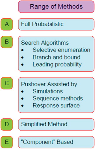
A full probabilistic method (Category A in Figure 1) is a structural system with multiple failure paths can be represented by a series of parallel subsystems where each sub-system represents a failure mode. In the case of complex structures such as fixed offshore platforms, where there is a very large number of possible failure paths. There may be a large number of participating structural components which makes this approach impractical. For this reason, research efforts have been focussed on the development of more efficient system-based reliability methods for these structures. Due to the significant computational demand associated with a rigorous system-based reliability analysis of an offshore fixed platform, a number of ‘search algorithms’ (Category B in Figure 1) have been developed (Onoufriou and Forbes 2001). The objective of these searching algorithms is to develop efficient methods for identifying the most dominant failure paths, which are then used to calculate the combined system probability of failure. Such methods include the branch and bound method, the selective enumeration technique, and the marginal probability and leading probability method.

There are some limitations associated with these searching methods (Category B in Figure 1). The branch and bound method is computationally very expensive when applied to large structures such as offshore fixed platforms. One method of identifying the most dominant failure path is by performing pushover analysis (Category C in Figure 1). This analysis will identify the deterministically most critical elements but will not take into account the effect of possible variations in component strength that may result in different sequences of failure and different combination of elements. Simulation methods were used in combination with pushover analysis to address these possible variations and their effects. The difficulty associated with this approach is the limiting number of simulations that can be performed given the size of the problem and the high computational demands. Although this is not a practical approach for reliability assessments of fixed offshore platforms, the studies undertaken using this method have produced the same useful conclusions and guidelines for simpler approaches (Onoufriou and Forbes 2001). It was observed that the system capacity can be related directly to the base shear force and can be estimated without taking into account the uncertainty of the load-pattern (Onoufriou and Forbes 2001). It was also concluded (Onoufriou and Forbes 2001) that reliability is dominated by uncertainties in modelling the sea state description, especially the significant wave height.

Another approach which also offers some refinement in the resistance variability prediction is to combine pushover analyses with the response surface method to obtain the distribution of structure resistance (University of Surrey 2000). A response surface method can be defined as an approximation of the mechanical behaviour of a system by simple functions, where these functions are obtained from sensitivity analyses of the system, thus providing sufficient information on the system behaviour. Once this response surface is suitably defined, any advanced probabilistic method for reliability analysis can then be applied. For the response surface method, the analysis generated a failure surface by systematically varying each of the important basic variables in turn about their mean values and determine the ultimate strength in each case via a pushover analysis or similar. By fitting an equation to this surface, a strength model is created. It is a function of the basic resistance variables and so can be readily input into a reliability analysis. The choice of basic variables and modelling accuracies used to create a response surface will be influenced by whether their mean values and/or uncertainties (i.e. coefficient of variance or COV) affect the reliability outcome. Where the variable can be treated as deterministic, it need not appear as a variable in the response surface. Its deterministic value, however, may be required in the generation of the surface.

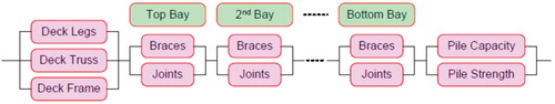
A simplified system-based reliability method (Category D in Figure 1) was developed based on a series system where the structural components in the series were the deck, each platform bay and the foundation. As shown in Figure 2, within each component, there were parallel elements including deck legs, braces, joints and piles. In order for the component to reach failure, all the parallel elements must have failed. To compute the probability of failure of a platform, each of the conditional probabilities (conditional on wave height) of failure were multiplied by the probability of occurrence of sea states that would generate expected maximum wave heights (equal to the long-term distribution of the expected maximum wave height for the location) and then sum.

Figure 2. Simplified system-based reliability methods.

Various studies performed so far indicate that the ‘component’-based approach (Category E in Figure 1) where the whole structure is treated as a component, with either deterministic resistance or an associated coefficient of variation (COV), is suitable to quantify the probability of system collapse of a fixed offshore platform. Based on this approach, it is proposed that with an accurate representation of the resistance, a good non-linear model and a competent engineer/analyst, it is possible to reduce significantly the modelling uncertainties associated with the resistance. It is also suggested that with an equally good loading model it is possible to predict values that can begin to be interpreted in an absolute sense to form the basis for decision making. This approach is a clearly defined method with potential for application in design and reassessment of fixed offshore platforms. The structural system reliability analysis method that was used for the system-based calibration of North West European annex (University of Surrey 1998) environmental action factor for ISO fixed steel offshore platform Code 19902 (ISO 2007) adopts this category of ‘component’-based approach. This ‘component’-based method has also been used in this study to perform system-based calibration of extreme environmental action factors for all three regions of Malaysia waters.

4. Uncertainties and sensitivity

Structural reliability is concerned with the rational treatment of uncertainties in structural engineering design and the associated problems of rational decision making. Uncertainty is generally categorised into three groups: physical uncertainty, statistical uncertainty and modelling uncertainty.

Physical uncertainty arises from the actual variability of physical quantities, such as loads, material properties and geometric dimensions. The statistical uncertainty arises due to a lack of information. The model uncertainty occurs as a result of simplifying assumptions, unknown boundary conditions and as a result of the unknown effects of other variables and their interactions that are not included in the structural analysis model. Modelling uncertainties can also arise due to the uncertainty from imperfections and idealizations made in physical model formulations for load and resistance, and from choices of probability distribution types for the representation of uncertainty. It can be described as random factors in a physical model used for representation of load or resistance quantities and can be derived by the ratio between the true quantity and the quantity as predicted by the model. A mean value not equal to 1.0 expresses a bias in the model. The standard deviation expresses the variability of the predictions by the model.

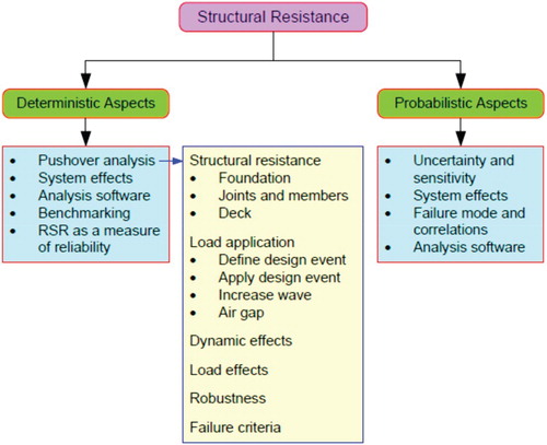
There are various probabilistic and deterministic aspects associated with the structural resistance side of a system reliability analysis, as shown in Figure 3. Such aspects need to be addressed in system-based reliability assessments. The primary uncertainties involved in the structural resistance are associated with member and joint strength of the jacket structure, foundation stiffness and capacity and deck strength. There are also various aspects of modelling uncertainties. A potentially large source of modelling uncertainty is associated with the foundation representation. This is associated both with the foundation model and the soil parameters used which creates an incompatibility between the accuracy of the structure and that of foundation models.

Figure 3. Structural resistance aspects.

The yield strength study (University of Surrey 2000) shows that the greater the increases in yield strength, the higher the reserve strength ratio (RSR) exhibited and conversely, the lower the yield strength, the lower the RSR value shown. It was concluded (University of Surrey 2000) that as the yield strength was increased, a proportional increase in the RSR was exhibited. If the yield strength was increased from −3 to +3 of standard deviation, there was an overall increase in the RSR of approximately 13%. As the yield strength is increased, the number of plastic hinges forming in the foundation piles decreases as the strength in the piles is also increased, resulting in a jacket only failure mode. However, as the yield strength was decreased, the failure mode shifted from jacket dominated to mixed mode failure. Foundation capacity and reliability were once identified as an important issue in structural system reliability analysis. Similar to the yield stress issue, effects of foundation stiffness and capacity on the structural system capacity were studied deterministically (University of Surrey 2000). The results (University of Surrey 2000) have shown that an increase in the pile capacity caused an increase in the RSR and where there was a decrease in pile capacity there was also a decrease in the RSR. However, as the foundation capacity was increased, only slight increases in the RSR were exhibited. The change in RSR, therefore, was smaller for those runs with increased foundation capacity than those runs with a decreased foundation capacity.

Pushover analysis plays an important role in some rigorous structural system reliability analysis of offshore fixed platforms to identify critical loading modes. The prediction of the ultimate capacity of a system is an essential step in the assessment of a structural system and hence, reliability. Significant modelling uncertainty exists. Variabilities that are introduced to pushover analysis and thus system reliability include definition of failure criteria, the competence of the users and human errors associated with the modelling. Some variation is associated with the actual software used, but in most cases, the main source of uncertainty was related to the use of the software rather than its specific characteristics. This type of uncertainty will reduce as the competence of the user increases.

System effects in fixed offshore platforms can be divided into two groups: deterministic effects which relate to the redundancy of the system and effects relating to the randomness of the member capacity. Studies to date (University of Surrey 2000) have shown that the most important system effect contribution comes from the deterministic aspect, i.e. the redundancy of the system, while probabilistic aspects of failure modes and correlation effects make only a small contribution. This is due to a high correlation between failure modes which is observed in fixed offshore platforms. This points towards the ‘component’-based approach, with a deterministic resistance representation, or a coefficient of variation (COV) of the order of 10%, as being an appropriate representation within a system reliability assessment. Furthermore, this highlights the reserve strength ratio (RSR) as being an important indicator of the system reliability of a structure. RSR forms one of the main criteria for re-qualification of fixed steel offshore platforms.

The predictions of wave loads were subject to uncertainties due to the inherent randomness in the wave process, uncertainties in the sea state parameters and uncertainties in the prediction of wave forces for any given sea state. Of the loading variables, the wave height was found to be the most dominant variable, followed by the wave period and then the drag coefficient. The dominance of these loading variables was found to introduce high correlation between the failure events of different components within a failure path and between failure paths. Structural system reliability analyses of fixed offshore platforms performed by different individuals and organisations have concluded that, despite the fact that there would appear to be large uncertainties in the resistance models, these do not appear to have a large impact on the reliability assessment as this is dominated by the uncertainties in the loading. For offshore structure, in general, the uncertainties in prediction of wave force were greater than the variability in prediction of system capacity.

5. Probabilistic modelling of structural resistance

As mentioned previously, under the implement of ‘component’-based method, the statistics of structural resistance is characterized in terms of reserve strength ratio (RSR). Instead of using the directly collated value of RSR that including large uncertainties associated the RSR results from pushover analyses, a theoretical RSR model is adopted to characterise the minimum RSR, reflecting fully optimised designs to the ISO 19902 (2007). In this model, a direct relationship between RSR and the environmental load factor is developed, and thus the partial action factor can be calibrated aiming for target reliability.

Reserve strength ratio (RSR) of a fixed platform is defined as the ratio of environmental load that causes the platform to collapse over the original design environmental load. The theoretical RSR model was developed based on the sources of reserve strength that exist in a fixed offshore platform, which causes the actual strength being above the design strength. These sources of reserve strength that exist in a fixed offshore platform include

• Explicit code safety factor, or margin of safety ($MOS$),

• Implicit code safety factor, or $ICSF$, such as empirical equations for joints and members,

• Actual material strength or material factor, $MF$, which is often high than the minimum specified value used in the design,

• System redundancy ($SR$),

• Steel work included for temporary phases, e.g. transportation and/or installation, and

• Engineering practice of operating companies, etc.

RSR of an offshore platform is evaluated using non-linear finite element (FE) analysis, often termed pushover analysis. Typically, the analysis is undertaken by applying the gravity loading as an initial load step. The environmental design load is then applied to the model and is factored incrementally until the ultimate strength of the structure is reached. The fundamental of using ‘component’-based method to calibrate the partial action factor is that the theoretical RSR model has direct relationship to the extreme environmental action. This is based on the fact that only the environmental loads are scaled in a pushover analysis. This phenomenon is designated as ‘$PDPE$ factor’, where $P_D$ is the unfactored gravity load and $P_E$ is the unfactored environmental load for fully utilised member. The $PDPE$ factor occurs because part of the member strength arises from code strength requirements for gravity load and part from code strength requirements for environmental load. The margins on the gravity load allow the environmental load to be increased beyond its factored values before failure occurs.

It is, therefore, possible to calculate the theoretical RSR by multiplying the individual contribution factors given above, such as (1) $RSR=MOS\cdot ICSF\cdot MF\cdot SR\cdot PDPE.$(1)

By defining a parameter of $RS{R}^{\mathrm{\prime }}$ as (2) $RS{R}^{\mathrm{\prime }}=ICSF\cdot MF\cdot SR.$(2)

Equation (1) can be rewritten as (3) $RSR=MOS\cdot RS{R}^{\mathrm{\prime }}\cdot PDPE.$(3) Factors $MOS$ and $PDPE$ can be derived from the ISO 19902 Code (2007) and University of Surrey (1998) for detailed derivations; while $RSR\mathrm{\prime }$ can be obtained from pushover analyses of fixed platforms.

Pushover analyses were performed on the six selected representative platforms. A total of 110 existing ultimate strength assessment reports provided by PCSB were also review in order to determine the ranges of the parameters used in the theoretical model for the minimum RSR calculation. Among variables determining the system structural resistance, the parameter of most significance to response modelling within reliability assessments is the yield strength of the structural material. The expected (average) material strength is around 20% higher than the nominal yield strength for 36 ksi steel and 15% for 50 ksi steel. Based on the review on the modern jacket structures installed after year 2000, all used structural steel with a specified minimum yield stress of 50 ksi. A material factor ($MF$) ranging from 1.13 to 1.15 was used in the structural system reliability analysis. Table 9 summarises the range of parameters used in system reliability analysis. The parameter $RS{R}^{\mathrm{\prime }}$ was defined with a lower bound, upper bound and typical values which were taken as the averages of those derived from pushover analyses results for each region offshore Malaysia.

6. Probabilistic modelling of environmental load

Offshore platforms are installed in a fluid environment. The load effect is evaluated using hydrodynamic and aerodynamic concepts. Morison’s equation is generally applied to evaluate the effect of hydrodynamic loads on fixed offshore platforms. A review of the literature reveals that there exist two categories to obtain the probabilistic modelling of environmental load:

• Category 1: Parametric response surface fitted with basic environmental parameters at the vicinity of ‘design point’, and

• Category 2: Response-based load statistics module (LSM)

Category 1 method is to find an expression that relates the basic environmental parameters and the load on the fixed platforms (e.g. base shear). Studies (Tarp-Johansen 2005) have shown that, for drag-dominated structures, the hydrodynamic response surface model is quadratic, given that the wave height is raised to the second power. The expression, in general, takes the following form: (4) $\begin{array}{rl}F& =a\cdot H_{\text{max}}^2+b\cdot H_{\text{max}}+c\cdot V_c^2+d\cdot V_c+e\\ & \cdot V_w^2+f\cdot V_w+g\end{array}$(4) where

• F =  environmental load on the offshore platform (e.g. base shear),

• H_max =  maximum individual wave height,

• V_c =  current speed,

• V_w =  wind speed, and

• a, b, c, d, e, f, g = deterministic constants

In order to determine the response surface, the uncertainties of environmental parameters are first evaluated based on the sea state data. The evaluation of the long-term distribution of the environmental parameters is executed using extreme value statistics. The most typical probability distributions used in the evaluation of the offshore environmental annual extremes are Gumbel or Weibull distributions. In practice, the observed metocean data, during a certain period is fitted to these theoretical distributions, the best-fit curve is then selected.

The load exerted on a jacket type structure is assumed to be due to the single highest wave (H_max) in a sea state or storm. H_max can be achieved by applying a factor to H_s, where the applied conversion factor is a random variable that can be modelled using a normal distribution. The distribution of significant wave height is commonly modelled by a 2- or 3-parameter Weibull distribution or a Gumbel distribution.

The distribution of wind speed of given significant wave height is assumed to be 2-parameter Weibull distribution. This distribution has been found to satisfactorily represent the parent distribution of wind speed at many locations. The wind speed is conditional on H_s. The 2-parameters of Weibull distribution of wind speed are expressed as functions of significant wave height H_s.

The condition distribution of peak energy period T_p is assumed to be log-normal distribution with mean and standard deviation that can be defined as a function of significant wave height H_s. The wave period associated with the maximum wave height T_ass is typically related quite closely and deterministically to T_p with a reasonable calculation of T_ass = 0.93T_p.

The response surface method has been used for structural reliability analysis of offshore fixed platforms located in different regions including Gulf of Mexico, offshore Trinidad, North Sea and offshore Malaysia (Nichols et al. 2014), (Onoufriou and Forbes 2001; Tarp-Johansen 2005; Wang et al. 2007). This method was also used for the component-based calibration of extreme environmental action factors for offshore Malaysia (Nichols et al. 2014). During the component-based calibration (University of Surrey 2000), FORM was used for the derivation of the reliability index. An iterative approach was adopted to ensure that the design point locates on the fitted response surface.

Different to Category 1 response surface method where the statistical analysis is performed to the metocean parameters, the Category 2 response-based load statistics module (LSM) approach first derives the environmental load (response) using selected storms from hindcast data, and process statistical analysis of the load (response) to determine the short-term and long-term distribution of the environmental load (response). Figure 4 outlines the steps to establish the probabilistic model of environmental load using the response-based load statistics module (LSM) approach (Tromans and Vanderschuren 1995).

Figure 4. Outline of response-based load statistics module approach.

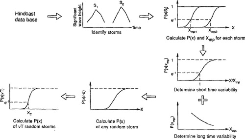
The first step of the LSM approach is to identify storms in the hindcast time series by examining the time history of significant wave height H_s (Tromans and Vanderschuren 1995). All time intervals with H_s less than 30%–40% of the largest values are discarded. This reduces the data size and also breaks the hindcast database into ‘storms’. For storms with twin peaks as shown in Figure 4, two storms are formed by breaking at the trough between the two peaks should the trough value be less than 80% of the lowest peak.

The second step of the LSM approach is to determine an empirical distribution of extreme response (load) of each storm identified in Step 1 (Tromans and Vanderschuren 1995). An identified storm is divided into 3-h intervals with the peak of storm at time 0. Each 3-h interval has a representative significant wave height and different number of individual waves. Each individual wave height in a 3-h interval has the probability distribution of Rayleigh. Similar to the response surface method (Category 1), a generic load model (GLM) is fit for each individual wave. For drag-dominated structure, the following generic load model was used in reference (Tromans and Vanderschuren 1995) (5) $\begin{array}{rl}F& =A_1{V}_c^2+A_2{V}_{c}a{T}_z\varphi \cos ({\theta }_c)+A_3{\varphi }^2{a}^2\\ & +A_4\frac{V_c\varphi a^2\cos ({\theta }_c)}{T_z}\\ & +A_5\frac{{\varphi }^2{a}^3}{T_z^2}+A_6{V}_w^2\cos ({\theta }_w)\end{array}$(5) This generic load model (GLM) omitted the inertia load and considered the wave direction spreading factor (φ), angle between current and dominate wave direction (θ_c) and the angle between wind and dominate wave direction (θ_w). V_c, V_w and a in Equation (5) represent the integrated current speed, wind speed and crest height, respectively. The dominant term in the above GLM was found to be $A_3{\mathrm{\varnothing }}^2{a}^2$, which ensures the adoption of asymptotic behaviour of extreme waves to extreme response.

The third step of the LSM approach is to perform short-time statistics analysis by renormalising all the distributions of the most probable extreme individual load (Tromans and Vanderschuren 1995). It has been observed that each short-time variable of the most probable extreme individual load is almost identical for all the large storms within a directional sector. After deriving the short-time statistics, the fourth step of LSM approach is to undertake long-time statistics analysis, during which the most probable extreme individual loads of large storms in a given directional sector are used to fit a probability density function (Tromas and Vanderschuren 1995). In general, Weibull, Gumbell, Fretchet or generalised Pareto distributions (GPD) can be used for the fit.

In the present study, the LSM approach (Category 2 method) was used for probabilistic modelling of environmental load. During the application of the LSM approach, it was agreed among PCSB and consultant that a ‘decision tree’ was implemented as how to establish the probabilistic modelling of environmental load, as illustrated in Figure 5. The first option is to establish a continuous equation of GLM, e.g. Equation (5) and use either FORM/SORM or Monte Carlo method for reliability analysis. The second option is to establish the GLM in a discrete form (i.e. one-to-one relationship between metocean parameters and environmental load) and then use Monte Carlo simulation for reliability analysis.

Figure 5. Illustration of ‘decision tree'.

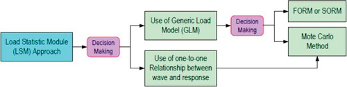
In the present study, option 1 with FORM was adopted based on the results achieved. An updated GLM was developed to include wave-in-deck effects, which is a major parameter that leads to the collapse of a fixed offshore structure during extreme storm events.

7. Hindcast databases

SEAFINE databases include the wave and wind hindcast data. HYCOM databases are the hindcast data for current. The Oceanweather Report (2008) describes the derivation of the SEAFINE hindcast data including its validation, while the Oceanweather Report (2012) reports the validation of the HYCOM data. The databases were provided by PCSB in text file format and were imported in MS Excel and MATLAB software program for further processing. One of the main effects of current is that it causes a Doppler shift on wave periods. Since the correct period to use with all periodic wave theories is the intrinsic wave period, care is required when interpreting wave periods as to their basis. For fixed structures, wave period recorded or from drifting instruments is the intrinsic period. When interpreting hindcast wave data, it has to be scrutinised to check whether the validation, if any, is generally derived from either fixed locations, when the apparent period is effected using measurements from fixed or from floating instruments and then, whether any necessary adjustments have been made. However, it was stated in the MMC Report (2014) that attempts to ascertain the basis of the HYCOM data proved unsuccessful, so it was not known whether any adjustments are in fact necessary.

ISO 19901-1 (2015) provides appropriate equations to account for the Doppler effect, which requires the input velocity to be specified as the value in-line with the direction of wave propagation, provided the current profile is uniform over the water depth. The MMC Report (2014) also pointed out the uncertainties associated with trying to implement the ISO 19901-1 (2015) Doppler effect based on the use of depth-averaged current.

The generic load model (GLM) was used in the present study to transform wave statistics to response statistics. To establish a GLM, environmental loads (wave, current and wind loads) are generated based on appropriate metocean parameters. The generated environmental loads are then used to fit the parameters that define the GLM. The hindcast database can be directly used as samples of metocean parameters. However, direct samples from hindcast data would not result in any wave-in-deck load information since the waves are not high enough to reach the deck. The purpose of pre-processing the hindcast database is to understand the statistical distributions and relationships of various metocean parameters.

8. Annual probability of distribution of extreme load

This section illustrates the response-based load statistics module (LSM) approach (Tromans and Vanderschuren 1995, 2001) adopted for the derivation of the statistics of both extreme wave height and extreme environmental load for all six locations within the three PCSB operating regions offshore Malaysia. The Tromans’ model proposed the LSM approach and uses the most probable extreme individual wave (or structural response) of the storm history rather than the peak significant wave height to identify a storm. The most probable extreme individual wave height (or structural response) is a function of several of the most severe sea states of the storm, which thus uses more of the data and should be less sensitive to noise (Efthymiou et al.1996; Tromas and Vanderschuren 2001).

8.1. Storm identification

The process begins with meteorological and oceanographic (metocean) data taken from the SEAFINE/HYCOM hindcast database provided by PCSB, following the detailed procedures described by Tromans and Vanderschuren (1995, 2001). Directional sectors with severe seas are identified to be between 150 and 240 degree clockwise from the True North, including around 250 identified storms per location in three regions offshore Malaysia. Each storm event is subdivided into a series of 3-h intervals, which becomes the basic unit in which the statistics analyses were performed on. It should be noted that the weather in Malaysia is dominated by Monsoons whose seasons extend for some four months. The wind patterns that generate monsoons are unlike those cyclic winds that create hurricanes in the North Sea or Gulf of Mexico. The monsoon wind pattern and, therefore, the corresponding sea state patterns, prevail for much longer periods than hurricane. Typical storms identified from the hindcast data last for over 200 h.

8.2. Probability distribution of extreme wave height

As discussed in Section 8.1 during storm identification, each storm has been divided into a number of 3-h intervals. The 3-h interval time series can be treated as statistically stationary. Each 3-h interval consists of certain numbers of individual waves. Similar to the work done in the JIP for the North Sea (Tromans and Vanderschuren 1995), consider the ith interval, which has a significant wave height of $H_{si}$, the wave height or crest elevation of an individual wave height in this ith interval is assumed to be under the Rayleigh distribution (6) $P(H|H_{si})=1-exp\left\{-2{\left(\frac{H}{H_{si}}\right)}^2\right\}=1-Q_i,$(6)

If the ith interval of the storm has $n_i$ numbers of individual waves, then the distribution of the largest wave height of these $n_i$ waves is (7) $P(H|i)=[P(H|H_{si}){]}^{n_i}\approx exp(-n_i\cdot Q_i).$(7)

If the intervals of the particular storm are numbered over $-I\le i\le J$, where $i=0$ is the peak of the storm, then the probability distribution of the largest wave of the whole storm (denoted as s) is (8) $P(H|s)=\prod _{-I}^{J}P(H|i)=exp\left\{-\sum _{i=-I}^J(n_i\cdot Q_i)\right\}$(8) The above procedure is repeated for all identified storms. It can be observed from Equations (6)–(8) that – with wave heights become greater than two times the significant wave height, i.e. $H\ge 2H_{si}$, would have a corresponding cumulative probability very close to unity.

The ‘short-time’ statistics of a storm describes the probabilistic behaviour of the extreme wave within a storm. The probability distribution of the largest wave of an identified storm, $P(H|s)$ as given in Equation (8) should converge to an asymptotic form, conditional only on $H_{mp}$, which is the most probable value of the extreme individual wave height of the identified storm [21] (9) $P(H|H_{mp})=exp\left\{-exp\left[-\ln (N)\cdot \left[{\left(\frac{H}{H_{mp}}\right)}^2-1\right]\right]\right\}$(9)

In LSM approach, $H_{mp}$ (rather than the peak $H_s$) is used to characterise each identified storm. The $H_{mp}$ of each storm is easily obtained since P(H|s) = 1/e when $H=H_{mp}$. A set of $H_{mp}$ sample values were determined by calculating for each identified storm. This was achieved by fitting Equation (8) to the following function: (10) $P(H|s)\sim exp\{-exp(-A{H}^2+B)\},$(10) where the constants $A$ and $B$ were determined using the least-square method. With the above fitting for the probabilistic distribution of the largest wave of a storm, $H_{mp}$ were determined for all identified storms as (11) $H_{mp}=\sqrt{B/A}.$(11)

The coefficient ln(N) in Equation (9) was calculated for all identified storms as (12) $\ln (N)=B.$(12)

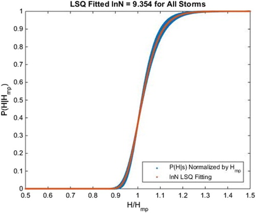
The coefficient ln(N) was determined to have a value around 9.6 for extreme waves in all three regions of Malaysia waters. Figure 6 presents the ‘short-time’ statistics of extreme wave heights in the Platform 1 location in Region A, as an example. It has been observed that the normalised wave height distributions turn out to be almost identical for all large storms.

Figure 6. Short-time probability distribution of normalised extreme wave height in Platform 1 location.

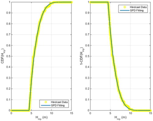
The specific of the ‘long-time’ statistics of storms is to determine a probability distribution of the most probable value of the extreme individual wave height, p(H_mp). In this study, both the Weibull and the generalised Pareto distribution (GPD) are studied, and the GPD is adopted for the better fitting for the upper tail. The cumulative probability of GPD for a variable x is

(13) $\begin{array}{rl}& PD{F}_{GPD}(x)\\ & =\{\begin{array}{ll}\frac{1}{\sigma }{\left\{1+\gamma \frac{x-\theta }{\sigma }\right\}}^{-1-\frac{1}{\gamma }},& \sigma >0,\gamma \ne 0,1+\gamma \frac{x-\theta }{\sigma }>0\\ \frac{1}{\sigma }exp\left(-\frac{x-\theta }{\sigma }\right),& \sigma >0,\gamma =0\end{array}\end{array}$(13) Figure 7 illustrates the fitting of GPD distribution of $H_{mp}$ in the Platform 1 location in Region A, as an example.

Figure 7. Long-time probability distribution of extreme storms characterised by H_mp in Region A Platform 1 location.

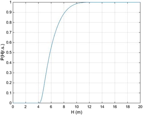
Combining the ‘short-time’ scale model given in Equation (9) with the ‘long-time’ scale model deduced from data fitting using GPD in Equation (13), one can obtain the distribution of extreme wave height of any random storm (denoted as $r.s.$): (14) $P(H|r.s.)={\int }_{H_{mpmin}}^{H_{mpmax}}P(H|H_{mp})\cdot p(H_{mp})d{H}_{mp}$(14) Based on the ‘short-time’ and ‘long-time’ variability, the extreme wave height distribution for a random storm, P(H|r.s.), can be obtained by numerical integration using Equation (14) from minimum to maximum most probable values used in the long-time variability fitting. Figure 8 shows the extreme wave height probability distribution for a random storm at the location of Platform 1 in Region A as an example.

Figure 8. The probability distribution of the extreme wave height of a random storm in Platform 1 location.

8.3. Generic load model (GLM)

The generic load model (GLM) is a tool that has been employed for each sea state to transform statistics of ocean surface elevation into load on fixed platforms. A one-to-one relationship is expected between statistics of ocean surface elevation and load on the structure. In addition to the derivation of GLM in a form of continuous numerical function, a discrete relation between ocean surface elevation and load on structure has also been considered in this study. However, to cover a very wide range of all sea state parameters, it may result in database that is impractically large. As a result, this study applied the GLM method in a form of continuous function for the transformation between wave motions and structural responses.

As an extension to the traditional GLM used for the North Sea, a modified GLM expression was theoretically derived for the base shear of drag-dominant structure with wave-in-deck force, using Morison’s equation. The derivation is based on the updated stick model shown in Figure 9. The bottom cylindrical member (stick model) represents the jacket structure, which was used in the traditional GLM derivation. The updated stick model has a second cylindrical member sitting on top of the bottom member, which represents the deck structure. The deck-to-jacket diameter ratio shown in Figure 9 is 1.5. This ratio was determined from a survey of the ratio of wave-in-jacket load over the wave-in-deck forces on all PCSB fixed platform fleet.

Figure 9. Model for wave-in-deck force derivation.

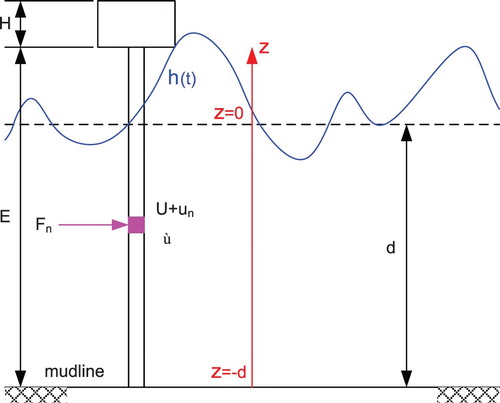
The extended GLM that includes wave-in-deck forces was theoretically derived based on Morrison Equation for drag-dominant structures. The base shear of drag-dominant structures can be expressed in terms of crest elevation, $a$, directional spreading factor, $\varphi$, zero up-crossing period, $T_z$, depth-integrated current, $V_c$, wind speed, $V_w$, angle between mean wave and current, ${\theta }_C$, and angle between mean wave and wind, ${\theta }_w$, and can be written as (15) $\begin{array}{rl}F& =A_1{V}_c^2+A_2{V}_{c}a{T}_z\varphi \cos ({\theta }_c)+A_3{\varphi }^2{a}^2\\ & +A_4\frac{V_c\varphi a^2\cos ({\theta }_c)}{T_z}\\ & +A_5\frac{{\varphi }^2{a}^3}{T_z^2}+A_6\frac{V_{c}a\varphi \cos ({\theta }_c)}{T_z}+A_7\frac{{\varphi }^2{a}^2}{T_z^2}\\ & +A_8\frac{\mathrm{\nabla }{V}_c{a}^3\varphi \cos ({\theta }_c)}{T_z^3}+A_9\frac{\mathrm{\nabla }{V}_c{a}^2\varphi \cos ({\theta }_c)}{T_z^3}\\ & +A_{10}\frac{\mathrm{\nabla }{a}^4{\varphi }^2}{T_z^4}+A_{11}\frac{\mathrm{\nabla }{a}^3{\varphi }^2}{T_z^4}+A_{12}{V}_w^2\cos ({\theta }_w),\end{array}$(15) where $A_1$ to $A_{12}$ depend on the configuration of the structure and the wave attack direction and are the constant to be determined. A₁ to A₅ terms are identical to the original terms included in the traditional GLM expression, as given in Equation (5). A₆ and A₇ terms are the correction to drag forces on the bottom column member (jacket) above mean sea level (MSL) and underside the deck. A₈ to A₁₁ terms represent the correction to drag forces on deck, which is computed using the API methodology (2000). Drag force above MSL that is induced by current only is neglected. The constant $\mathrm{\nabla }$ is the stretching parameter, with a value of 0.3 A12 Term is the wind force, which is also identical to the corresponding term in the traditional GLM (A₆ term in Equation (5)).

Determination of the $A$-parameters in GLMs was achieved by generating base shear forces using sets of metocean parameters, which were then used to fit the GLM expression given in Equation (10). The wave and current forces are calculated for the stick model using the Stream Function theory, including both inertia (though excluded in the right-hand side of the GLM equation) and drag components, in which case, the base shear force (left-hand side of the GLM equation) fitted by the GLM expression can be regarded as the real force on the stick model. It was assumed here that, for a new design of fixed offshore platform, the underside of the lowest deck main steel was set at the crest elevation of 1000-year return wave. This crest elevation can be determined using predicted 1000-year return extreme wave with positive tide and storm surge being accounted for.

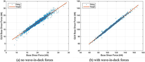
Figure 10 shows the loads obtained from the modified GLM plotted against the numerical calculations, for both cases without or with wave-in-deck forces, in at Platform 1 location in Region A offshore Malaysia. It can be observed that the fitting is very good for both cases. Unlike the fitting results for the North Sea North Sea (HSE 2003), Tromans and Vanderschuren (1995) and the Region A, it is observed that there is certain scattering effect in Regions B and C, which may be explained as a result of the multi-modal distribution of the angle between current and wave directions, ${\theta }_C$, which is widely spreading between 0 and 180 degrees in these regions.

Figure 10. Base shear load fitting of GLM for Platform 1 in Region A.

8.4. Probability of extreme load

Derivation of the probabilistic distribution of extreme environmental load is similar to that for the extreme wave as given in Section 8.2, by first establishing the ‘short-time’ and ‘long-time’ variabilities of the load. The generated GLM given in Equation (15) was first used to transfer the statistics of extreme wave to the statics of extreme environmental load, i.e. to generate a one-to-one relationship between wave crest, a, and load F. Assuming wave height $H=2a$, Equations (6) and (7) can be expressed for load F using the a and F relation determined from GLM. Similar to Equation (8), the probability distribution of the largest load of an identified storm (s) can be written as (16) $\begin{array}{r}P(F|s)=\prod _{-I}^{J}P(F|i)=Exp\left\{-\sum _{i=-I}^J[n_i\cdot Q(F_i^{-1}(F)|H_{si})]\right\}.\end{array}$(16) The above $P(F|s)$ calculations were repeated for all identified storms.

The ‘short-time’ statistics of load describes the probabilistic behaviour of the extreme peak structural response within an identified storm. Similar to the ‘short-time’ statistics of the extreme wave, $P(F|s)$ of an identified storm as given in Equation (16) should also converge to an asymptotic form, conditional only on the most probable extreme individual load within an identified storm, $F_{mp}$, and has the form of (17) $\begin{array}{r}P(F|F_{mp})=exp\left\{-exp\left[-\ln (N)\cdot \left[{\left(\frac{F}{F_{mp}}\right)}^C-1\right]\right]\right\}\end{array}$(17) where C is a constant with a value equal or greater than 1.0 due to the inclusion of wave-in-deck loads.

Similar to the derivation of $H_{mp}$ in Section 8.2, the ‘short-time’ statistics of load can be achieved by fitting Equation (17) to the following function (18) $P(F|s)\sim exp[-exp(-A{F}^c+B)].$(18) where A, B and C are the constants to be determined. Constant C is the same as that in Equation (17).

With the above fitting for the probability distribution of the largest response of a given storm, $F_{mp}$ values were determined for all identified storms as (19) $F_{mp}=\sqrt[c]{B/A}.$(19)

The parameter $\ln (N)$ values in Equation (17) were calculated for all identified storms as (20) $\ln (N)=B.$(20)

In this study, a sensitivity study was performed on the value of C. It is observed that all constant C value studied give very good fitting with the asymptotic expression for typical storms. A different constant value of C would result in a different value of coefficient ln(N), fitted by the least-square method. In this case, a value of 1.0 is finally adopted in the study, and the corresponding $\ln (N)$ coefficients for six platform locations are listed in Table 10.

Table 10. Statistical value of $\ln (N)$ for extreme load.

Region	Platform	LSQ fitted value
A	1	18.03
	2	18.53
B	3	20.17
	4	20.29
C	5	21.46
	6	20.74

The specific of the ‘long-time’ statistics of the extreme load is to determine a probability distribution of the most probable value of the extreme individual load, $p(F_{mp})$. There is no theory to indicate the appropriate form of this distribution. The sample values of $F_{mp}$ calculated for each identified storm do not directly provide information about the rarer, more severe storms with return periods greater than the duration of the original time series in the hindcast data. To predict the upper tail of the distribution, it is necessary to make some assumption about the ‘true’ distribution that the data obey.

Undoubtedly, there is modelling uncertainty in fitting probability distributions of the $F_{mp}$ data. There exists method for estimating modelling uncertainty in fitting distributions to data. However, they rely on the fact that one thinks he knows what distribution we should be fitting. Modelling uncertainties increases for the distributions with more degrees of freedom since more parameters need to be fit. Thus, the choice of distribution, exponential, Weibull or the GPD is very important and has major influence on the results.

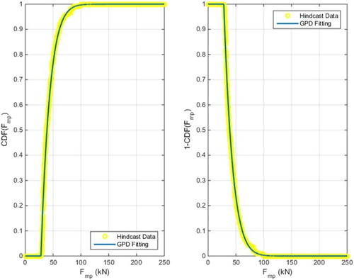
In this study, two types of distributions were tested for fitting the distribution of $F_{mp}$, which are Weibull distribution and generalised Pareto distribution (GPD). It has been found that GPD provided an almost exact fit for $F_{mp}$, especially for the fitting of the tails, as shown in Figure 11 for Platform 1 in Region A as an example.

Figure 11. GPD of probability and exceedance of $F_{mp}$ for Platform 1 in Region A.

Combining the ‘short-time’ scale model, $P(F|F_{mp})$, given by Equation (17), with the ‘long-time’ scale model, $p(F_{mp})$, deduced from data fitting using GPD, one can obtain the distribution of the extreme response of any random storm (denoted as $r.s.$) (21) $P(F|r.s.)={\int }_{F_{mpmin}}^{F_{mpmax}}P(F|F_{mp})\cdot p(F_{mp})d{F}_{mp},$(21) where $F_{mpmin}$ and $F_{mpmax}$ are the minimum and maximum values of $F_{mp}$, respectively, that are used to fit the probability distribution of the most probable extreme individual load in a storm, $p(F_{mp})$.

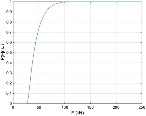
The extreme load distributions for a random storm were derived through numerical integration using Equation (21). Figure 12 illustrates the extreme response distribution of a random storm for Platform 1 in Region A as an example.

Figure 12. Extreme load CDF for Platform 1 in Region A.

The mean arrival rate of random storms can be estimated from the sample as (22) $\hat{v}=\frac{k+1}{\tau },$(22) where k is the number of $F_{mp}$ samples that used in the fitting of $F_{mp}$, and $\tau$ the total duration of the time series of the hindcast database. Uncertainty in the arrival rate has no significant consequence as long as $k$ is reasonably large.

Treating storm arrivals as a Poisson process, the extreme wave of an interval T has the probability distribution of (23) $P(F|T)=[P(F|\text{r}.\text{s}){]}^{\hat{v}T},\text{for large }\hat{v}T.$(23) Numerical differential method was used to derive the probability density function (PDF) of the probability distribution given in Equation (23). The probability distribution of extreme loads with different return periods from 1-year to 10,000-year was developed for all six locations within three PCSB operating regions. The determined extreme loads for different return periods are given in Table 11 for all six exemplary platform locations. Hazard curves were derived by normalising the extreme loads against that corresponding to 100-year return period. Figure 13 illustrates the hazard curves derived for all six locations within the three PCSB operating regions. Table 12 shows the ratio of 10,000-year return extreme load to that of 100-year return period, $F_{10K}/F_{100}$. These ratios are used to determine the annual probability distribution of extreme load normalised to the 100-year value, which is presented in Section 8.5.

Figure 13. Normalised extreme loads.

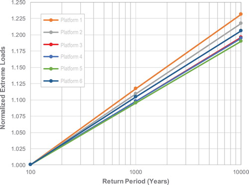
Table 11. Extreme loads for different return periods.

Region		A		B		C
Platform location		1	2	3	4	5	6
F (kN) for return period	1-year	66.28	59.06	31.80	32.23	39.38	43.15
	10-year	90.78	76.76	38.10	38.80	42.83	55.31
	50-year	102.11	84.51	41.23	42.00	51.88	61.23
	100-year	106.14	87.48	42.50	43.28	53.48	63.38
	1000-year	118.54	97.01	46.65	47.50	58.56	70.01
	10,000-year	130.69	106.46	50.81	51.71	63.63	76.43

Table 12. Ratio of 1000-year and 10000-year loads to 100-year load.

Region	A		B		C
Platform location	1	2	3	4	5	6
$F_{1K}/F_{100}$ ratio	1.117	1.109	1.098	1.096	1.095	1.105
$F_{10K}/F_{100}$ ratio	1.231	1.217	1.196	1.195	1.190	1.206

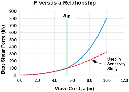
As shown in Figure 13, the environment hazard curves from Malaysian waters provide no expected obvious slope change at 1000-year return period, after when the wave-in-deck forces are kicked in. In order to explore the effects of wave-in-deck forces on the predicted extreme loads with different return period, a sensitivity study was carried out to produce another set of probability of extreme responses by following the same procedures described above. The only difference is that the sensitivity study excludes the wave-in-deck forces when transforming the wave statistics into response statistics using the generic load model (GLM), i.e. the relationship between wave crest elevation a and extreme load F, as shown in Figure 14. It has been observed that the results produced by the sensitivity study are almost identical to those presented above.

Figure 14. F versus a relation used for sensitivity study.

The reasons for the insignificant wave-in-deck force effects on the extreme response prediction may result from the following facts:

• The minimum deck height in this study was set as the 1000-year return crest elevation. This would lead to the case that the wave-in-jacket forces control the probability of the extreme loads. The effect of wave-in-deck force would be expected to become more significant should one lower the minimum deck height requirement.

• By setting the minimum deck height as the 1000-year return crest elevation, the value of the base shear force greater than which the wave-in-deck load plays a role is already very large. The wave crest height corresponding to this base shear load would have a probability of close to 1.0, based on the presumption that individual wave crest is following Rayleigh distribution.

• The distribution of the largest response of an identified storm, i.e. ‘short-time’ statistics, would converge to an asymptotic form, conditional only on its most probable value. With this asymptotic form distribution, the wave-in-deck forces would hardly contribute to the largest response of an individual storm.

8.5. Annual probability distribution of extreme load

Following procedures given in Sections 8.1–8.4, sets of extreme load statistics have been derived for all six locations within the three PCSB operating regions offshore Malaysia, which are well modelled by Gumbel distribution. The annual probability for base shear normalised against the 100-year return value is (24) $P(L^{\ast })=exp\left[-exp\left(-\frac{L^{\ast }-A}{B}\right)\right],$(24) where L is the extreme load with a certain return period; $L_{100}$ the 100-year return extreme load, $L^{\ast }$ the normalised extreme load, i.e. $L^{\ast }=L/L_{100}$. A and B are distribution parameters, which can be determined using the $L^{\ast }=L/L_{100}$ ratios given in Table 12. Table 13 presents the determined distribution parameters.

Table 13. Gumbel distribution of the annual probability of extreme loads.

Region	Region A		Region B		Region C
Platform location	1	2	3	4	5	6
$\text{Parameter A}$	0.7692	0.7835	0.8049	0.8056	0.8106	0.7945
$\text{Parameter B}$	0.0502	0.0471	0.0424	0.0422	0.0412	0.0447

9. System-based approach to calibration

With the theoretical RSR model, the limit state function or safety margin used in the structural reliability analysis was defined in Figure 15.

Figure 15. RSR model for a system approach to calibration.

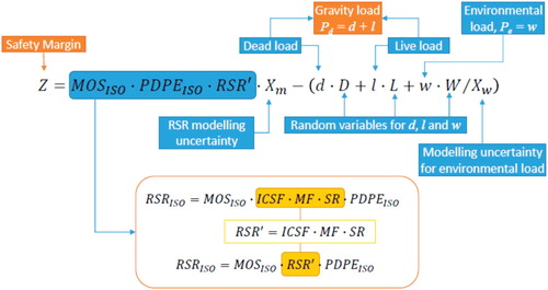
In Figure 15 X_m and X_w are the model uncertainties associated with RSR and environmental design loading evaluation, respectively. Lowercase d, l and w represent the proportions of unfactored dead, live and environmental load in the critical member initiating failure, i.e. d + l = P_d, load components due to environmental load; w = P_e, load component due to gravity load. The uppercase D, L and W are the random variables for dead, live and environmental load, respectively.

Compared with Equation (1), RSR is against the ISO 19902 Code (2007) and denoted as $RS{R}_{ISO}$, so as for the explicit code margin of safety ($MO{S}_{ISO}$) and $PDPE$ factor ($PDP{E}_{ISO}$). These factors are determined from the ISO 19902 Code (2007) (Cossa et al. 2013) as follows: (25) $MO{S}_{ISO}={\gamma }_{R_c}\cdot \frac{({\gamma }_d\cdot P_d+{\gamma }_w\cdot P_e)}{(P_d+P_e)},$(25) and (26) $PDP{E}_{ISO}=\left\{1+\left(1-\frac{1}{MO{S}_{ISO}\cdot MF\cdot ICSF}\right)\cdot \frac{P_d}{P_e}\right\}.$(26) where ${\gamma }_{RC}$ is 1.18 as the partial resistance factor for the member under axial compression. ${\gamma }_d$ and ${\gamma }_l$ are the partial load factors on dead and live loads, respectively. The gravity load factor is recommended to be ${\gamma }_d={\gamma }_l=1.10$ in ISO Code 19902 (2007), while the environmental partial load factor needs to be calibrated.

In addition to the established annual distribution of environmental loading, W, described in the previous section, the modelling of the uncertainty in resistance model and gravity loadings is the same as that adopted in system-based calibration for the North Sea extreme environmental partial action factor as summarised in Table 14. The failure function as well as the assigned probability distributions of basic variables are programmed into a fully calibrated in-house spreadsheet. Reliability analyses, using the first-order reliability method (FORM), are performed for a realistic range of structural systems based on a limited number of pushover analysis results and estimated upper and lower bounds for RSR, as listed in Table 15.

Table 14. Load and resistance model uncertainty probability distributions.

Basic variable	Distribution	Mean bias	SD
$X_m$	Log-normal	1.0	0.1
$X_w$	Truncated normal at ± 1.5 SD	1.09	0.18
W	Gumbel	$A+0.5772B$	$B\frac{\pi }{\sqrt{6}}$
D	Normal	1.0	0.06
L	Normal	1.0	0.1

Table 15. Ranges of parameters used in the system reliability study.

Parameters		MF	ICSF	SR	RSR'
Lower bound		1.13	1.00	1.04	1.18
Typical value	Region A	1.15	1.50	1.18	2.02
	Region B	1.15	1.45	1.06	1.76
	Region C	1.15	1.46	1.19	2.00
	Average	1.15	1.47	1.14	1.93
Upper bound		1.15	1.50	1.20	2.07

Note: $MF=$ material factor;

$ICSF=$ IMPLICIT CODE SAFETY FACTOR;

$SR=$system redundancy; $RS{R}^{\mathrm{\prime }}=ICSF\cdot MF\cdot SR$.

9.1. Individual reliability analysis results

To illustrate the reliability analysis results obtained and sensitivity of the basic variables, typical results for Platform 1 in Region A as an example are given in Table 16. In this calculation, the $RS{R}^{\mathrm{\prime }}$ has been assumed to be 1.93, which is the average of those derived from pushover analyses of selected exemplary platforms as given in Table 9. The environmental-to-gravity load ratio (P_e/P_d ratio) has been taken as 4.5 based on the survey of PCSB existing fixed offshore platforms, and the environmental (${\gamma }_w$) is 1.2. The value of RSR was calculated as 3.03.

Table 16. β-point values and sensitivities for Platform 1 in Region A.

Basic variable		β-point (x* value)	Sensitivity coefficient (α-factor)
Resistance	$X_m$	0.665	0.5235
Load model	$X_w$	0.841	0.2686
Environmental load	W	1.883	−0.8081
Dead load	D	1.007	−0.0142
Live load	L	1.018	−0.0237
Equivalent reliability index β (RSR = 3.03)			7.716

The equivalent values of reliability index (β) were calculated as 7.716, as shown in Table 13. Also shown are sensitivity coefficients (α-factors) along with the values of basic variables at the β-point, i.e. the most likely failure point. For all six platform locations, the most sensitive variable (with highest sensitivity coefficients) is the uncertainty in environmental load (W), followed by the uncertainties in RSR (X_m) and design load modelling (X_w). Dead and live loads (D and L) are of negligible influence on reliability.

The curvature of the failure surface was investigated at the β-point using second-rrder reliability method (SORM). No significant difference was observed from the reliability results from FORM. Therefore, FORM was considered adequate for the present purposes.

9.2. General reliability analysis results

On the basis of the range of $RS{R}^{\mathrm{\prime }}$ parameters defined, studies are carried out on the variation of reliability for typical jacket structures across a range of environmental-to-gravity load ratio (P_e/P_d) and for different environmental load factor (${\gamma }_w$). Figure 16 shows variation of reliability index (β) with environmental-to-gravity load ratio ($P_e/P_d$) for Platform 1 in Region A as a typical example. For each location, the reliability index (β) varies from approximately 12.0 for $P_e/P_d$ ratio of 1.0 to around 6.0 for cases dominated by environmental loading. However, for a particular $P_e/P_d$ ratio, the reliability index (β) varies by approximately 1.5 for all six considered platform locations when the environmental load factor is changed with a range of 1.00–1.40. It has been observed that the environmental-to-gravity ratio ($P_e/P_d$) has much greater effects on reliability than load factor (${\gamma }_w$).

Figure 16. β vs. ${\mathit{P}}_{\mathit{e}}/{\mathit{P}}_{\mathit{d}}$ ratio with different ${\mathit{\gamma }}_{\mathit{w}}$ for Platform 1 in Region A.

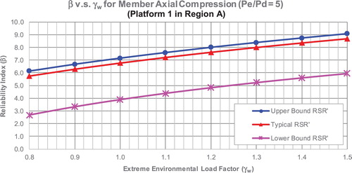
Figure 17 shows variation of reliability index (β) with environmental load factor (${\gamma }_w$) for a typical environmental-to-gravity ratio ($P_e/P_d$) of 5.0 due to different $RS{R}^{\mathrm{\prime }}$. The difference in reliability index (β) between the lower bound and upper bound is around 3.0, but the difference between a load factor (${\gamma }_w$) of 1.20 and 1.40 is only less than 0.80 for the same value of $RS{R}^{\mathrm{\prime }}$. The slope of the curves is small, which would make the selection of an environmental load factor (${\gamma }_w$) to achieve the required target reliability difficult on this basis.

Figure 17. β vs. ${\mathit{\gamma }}_{\mathit{w}}$ with different $\mathit{R}\mathit{S}{\mathit{R}}^{\mathbf{\prime }}$ for Platform 1 in Region A.

From the above discussion, it might appear that the vagueness or lack of confidence in the environmental-to-gravity ratio ($P_e/P_d$) means that there is uncertainty in the theoretical minimum RSR, and this in turn means that there is a lack of confidence in the reliability evaluate on this basis. However, RSR sensitivity will be lower in reality.

Structures with failure sequences initiated by members with low environmental-to-gravity load ratios, e.g. unfactored $P_e/P_d$ ratios less than 5.0, such as many legs, will tend to have low implicit code safety factor ($ICSF$) values since leg members tend to have low slenderness, that is they will be closer to the lower bound line. Whilst structures with classical brace failure mechanisms will often be initiated by members with high environmental-to-gravity load ratios, e.g. unfactored $P_e/P_d$ ratio of 5.0 or more, such members may be expected to have typical $ICSF$ values and consequently have values of $RS{R}^{\mathrm{\prime }}$ (and RSR) that are above the lower bound values. The transitional $P_e/P_d$ ratio of 5.0 is subjective but is believed to be a reasonable value.

10. System reliability analysis results summary

An annual target failure probability of 3.00 × 10⁻⁵ (β = 4.00) recommended by Efthymiou et al. (1996) was used during the calibration of North Sea environmental load factor. This value is within the range of the recommended annual target reliability in Eurocode (1993), Canadian Standard Association (CSA 1989), Det Norske Veritas (Veritas 1992) and Nordic Committee for Safety of Structures (NKB 1978). It is also used in this study as an example of annual target failure probability.

Figures 18 and 19 illustrate the comparison of reliability index (β) varying with environmental load factor (${\gamma }_w$) among the six platform locations in Malaysia waters for two typical cases, respectively. Figure 18 shows a representative case for platforms governed by gravity load with failure mechanism initiated by leg failures. In the calculations, an environmental-to-gravity load ratio ($P_e/P_d$) of 5.0 was used with a lower bound $RSR\mathrm{\prime }$ value. Figure 19 illustrates a representative case for platforms governed by the environmental load with failure mechanism initiated by brace failures. During the calculations, an environmental-to-gravity load ratio ($P_e/P_d$) of 25.0 was used with a typical $RSR\mathrm{\prime }$ value.

Figure 18. β vs. ${\mathit{\gamma }}_{\mathit{w}}$ Factor for different locations (lower bound $\mathit{R}\mathit{S}{\mathit{R}}^{\mathbf{\prime }}$).

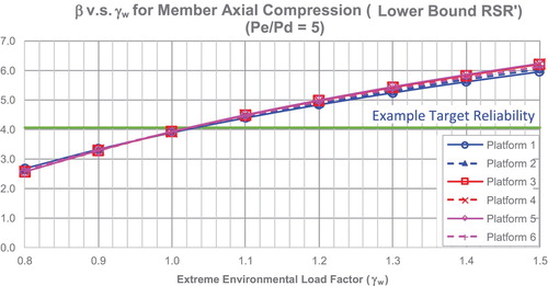
Figure 19. β vs. ${\mathit{\gamma }}_{\mathit{w}}$ factor for different locations (typical value of RSR’).

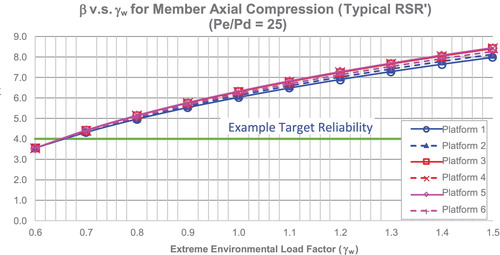
The following conclusions may be highlighted:

• Both cases show that the reliability index (β) varying with environmental load factor (${\gamma }_w$) are similar for the six platform locations, especially near the target reliability. It is considered that the three PCSB operating regions may use an identical partial action factor associated with extreme environmental loading.

• For the gravity load governed case, lower bound values are expected to control failure for many optimally designed structures; their failure sequence is initiated with leg members and the load in the failed members is dominated by gravity loading. An environmental load factor (${\gamma }_w$) of around 1.02 is required to achieve a target reliability of 3.00 × 10⁻⁵ (β = 4.00). The reliability assessed on the basis of theoretically derived lower bound values will be conservative.

• In general cases governed by environmental load, it has been recognised that structural failure is initiated with jacket braces and load in the failed members is dominated by environmental loading. The typical value of theoretical minimum RSR that are derived from pushover analysis results of selected exemplary platforms is, therefore, more applicable. This case recommends an environmental load factor (${\gamma }_w$) around 0.66 to achieve a target reliability of 3.00 × 10⁻⁵ (β = 4.00).

The failure probabilities evaluated from a reliability analysis are to some extent dependent on the level of Type II uncertainty included, which arises from lack of knowledge or information rather than the Type I uncertainty relating to the inherent natural variation in the environment, material, etc. One of the most significant sources of Type II uncertainty concerns the evaluation of the 100-year design load. The main system reliability analysis was undertaken with a COV of 16.5% for this variable. A study to assess the sensitivity analysis used a COV increased from 16.5% to 25%. The results from sensitivity analysis show that the difference in the evaluated annual failure probabilities is greater than an order of magnitude.

For reference, reliability analysis was also performed using the RSR derived from Platform 2 in Region A which has the lowest RSR value among the selected exemplary platforms, rather than the typical RSR value that was taken as the average of the assessed platforms. Results from structural reliability analysis show that an environmental load factor of 0.72 could achieve the same suggested annual target failure probability of 3.00 × 10⁻⁵ or an annual target reliability of β = 4.00.

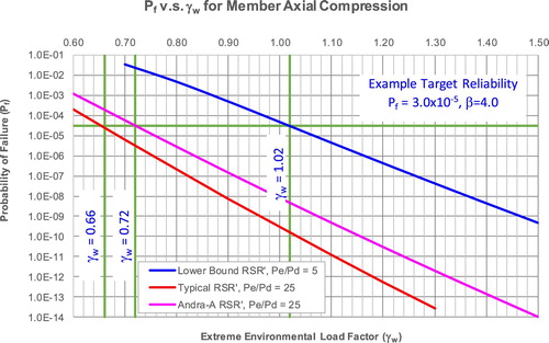
In order to assist the selection of appropriate environmental load factors and achieve a desired target annual reliability, plots of the target annual reliability and target annual failure probability varying with environmental load factors are presented in Figures 20 and 21, respectively. The environmental load factors recommended to achieve suggested target annual reliability or failure probability are also included in these figures.

Figure 20. Target annual β vs. ${\mathit{\gamma }}_{\mathit{w}}$ factor.

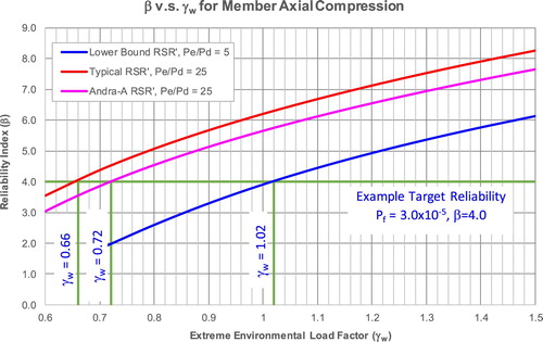
Figure 21. Target annual ${\mathit{P}}_{\mathit{f}}$ vs. ${\mathit{\gamma }}_{\mathit{w}}$ factor.

11. Conclusions and recommendations

Wave-in-deck forces can be included in the generic load model (GLM) transferring the wave motions statistics to structural response statistics. The effect of wave-in-deck forces on the prediction of extreme environmental load can be expected should one try other empirical distribution of individual wave height or crest and lower the minimum deck elevation requirements. The blue curves in Figures 20 and 21 correspond to low bound theoretical minimum RSR, which are representative of structures with failure sequences initiated by leg members. It is considered that in practice such structures are unlikely to occur. Using the blue curves will result in a very conservative estimation of annual reliability, i.e. an environmental load factor around 1.02 for a target annual failure probability of 3.00 × 10⁻⁵ (β = 4.00).

The red curves correspond to typical values of minimum RSR derived from the pushover analysis of selected exemplary platforms. They are representative of structures with failure sequence initiated by brace failure, which is recognised as more general in reality. For a target annual failure probability of 3.00 × 10⁻⁵ (β = 4.00), it is considered to be more applicable adopting an environmental load factor of 0.66. Based on the above observations and the results obtained using the lowest RSR value of Platform 2 in Region A (the pink curves in Figures 20 and 21), an environmental load factor of 0.70 is recommended for the design of offshore fixed platforms for all three operating regions offshore Malaysia using ISO 19902 Code (2007).

In essence, PCSB has used a more conservative value greater than 1.00 to represent their partial load factors for the environmental loading in Malaysian waters rather than 0.70 suggested within this study. This provides a greater comfort level to the Business, HSE and design engineers that there is some level of conservatism in the design of new fixed offshore structures, even though the target reliabilities have been exceeded. In conclusion, it is recommended that each global operating region, develop their environmental load factors based on their metocean data. This paper provides guidance on the methodology on how to do so and some of the key issues considered.

Acknowledgements

The authors of this paper will like to thank the management of PETRONAS’ Centre of Excellence, Technical Excellence team for their kind permission to publish this study.

Disclosure statement

No potential conflict of interest was reported by the authors.

ORCID

Riaz Khan http://orcid.org/0000-0001-6879-5290

Lee Luong Ann http://orcid.org/0000-0002-9691-5269

Nigel Wayne Nichols http://orcid.org/0000-0003-2900-7356

References

- API. 2000. Recommended practice for planning designing and constructing fixed offshore platforms – working stress design, API RP 2A-WSD 21st Edition, December 2000. Errata and Supplement 1, December 2002; Errata and Supplement 3, October 2005; Errata and Supplement 3, March 2008.
- Cossa NJ, Potty NS, Liew MS. 2013. Development of partial environmental load factor for design of Tubular joints of offshore jacket platforms in Malaysia. Open Ocean Eng J. 6:8–15. doi: 10.2174/1874835X01306010008
- [CSA] Canadian Standards Association. 1989. General requirements, design criteria, the environment, and loads, part 1 of the Code for the design, Construction, and installation of fixed offshore structures, Preliminary standard S471-M1989. Rexdale (Toronto) (ON): Canadian Standards Associations.
- Efthymiou M, van de Graaf JW, Tromans PS, Hiness IM. 1996. Reliability based criteria for fixed steel offshore platforms. Proceedings of OMAE Conference, Florence.
- Eurocode 1. 1993. Eurocode1: basis of design and actions on structures. Part 1: basis of design. Annex 2: partial factor design: background. European Standard.
- ISO 19901-1. 2005. Petroleumand natural gas industries – specific requirements for offshore structures – Part 1: Metocean design and operating considerations. International Organization for Standardization.
- ISO 19901-1. 2015. Petroleum and natural gas industries – specific requirements for offshore structures – Part 1: Metocean design and operating considerations. International Organization for Standardization.
- ISO 19902. 2007. Fixed steel offshore structures. International Organization for Standardization.
- MMC Oil & Gas Engineering Sdn Bhd. 2014. Hazard curves using SEAFINE wave data only. Document No. PCSB-A-1881/WO005/RP/0003, Rev A, February 2014.
- Nichols NW, Khan R, Rahman AA, Akram MKB, Chen K. 2014. Load resistance factor design (LRFD) calibration of load factors for extreme storm loading in Malaysian waters. JMET J. 13(2):21–34.
- Nordic Committee for Building Structures. 1978. Recommendations for loading and safety regulations for structural design. NKB Report No. 36.
- Oceanweather. 2008. SEAMOS – south fine grid hindcast (SEAFINE). Kuala Lumpur, Malaysia: Oceanweather.
- Oceanweather. 2012. SEAFINE 3d currents – validation of HYCOM 3D current model. Kuala Lumpur, Malaysia: Oceanweather.
- Onoufriou T, Forbes VJ. 2001. Developments in structural system reliability assessments of fixed steel offshore platforms. Reliab Eng Syst Safety. 71. doi: 10.1016/S0951-8320(00)00095-8
- Tarp-Johansen NJ. 2005. Partial safety factors and Characteristic values for combined extreme wind and wave load effects. J. Solar Energy Eng. 127. doi: 10.1115/1.1862259
- Tromans PS, Vanderschuren L. 1995. Response based design conditions in the North Sea: application of a new method. Proceedings of 27th Offshore Technology Conference, Paper OTC 7683, Houston, TX.
- Tromans PS, Vanderschuren L. 2001. Extreme environmental load statistics in UK waters. UK HSE Offshore Technology Report 2000/066.
- UK Health & Safety Executive (HSE) Research Report 087. 2003. System-based calibration of Northwest European annex environmental load factor for the ISO fixed steel offshore structures code 19902. Joint Industry Project Report.
- University of Surrey. 1998. Development of a structural system reliability framework for offshore platforms. JIP: structural reliability analysis framework for fixed offshore platforms, Document No. JHA003.
- University of Surrey. 2000. A review of system reliability considerations for offshore structural assessment. JIP: structural reliability analysis framework for fixed offshore platforms, Document No. JHA002.
- Veritas DN. 1992. Structural reliability analysis of marine structures. DNV Classification Note No. 30.6.
- Wang L, Chen K, Bucknell JR. 2007. Structural reliability assessment of offshore platforms under hurricane events. San Diego (CA): OMAE 2007-29313.