Real-time prediction of propulsion motor overheating using machine learning

ABSTRACT

Thermal protection in marine electrical propulsion motors is commonly implemented by installing temperature sensors on the windings of the motor. An alarm is issued once the temperature reaches the alarm limit, while the motor shuts down once the trip limit is reached. Field experience shows that this protection scheme in some cases is insufficient, as the motor may already be damaged before reaching the trip limit. In this paper, we develop a machine learning algorithm to predict overheating, based on past data collected from a class of identical vessels. All methods were implemented to comply with real-time requirements of the on-board protective systems with minimal need for memory and computational power. Our two-stage overheating detection algorithm first predicts the temperature in a normal state using linear regression fitted to regular operation motor performance measurements, with exponentially smoothed predictors accounting for time dynamics. Then it identifies and monitors temperature deviations between the observed and predicted temperatures using an adaptive cumulative sum (CUSUM) procedure. Using data from a real fault case, the monitor alerts between 60 to 90 min before failure occurs, and it is able to detect the emerging fault at temperatures below the current alarm limits.

KEYWORDS:

• overheating
• anomaly detection
• CUSUM
• linear regression
• temperature monitoring

1. Introduction

The common safety practice for prevention of overheating in marine electrical propulsion motors is based on physically mounted temperature sensors on the windings of the motor, often by resistor temperature detection (RTD) devices (IEEE Standard 3004.8 2016). An alarm is issued once the temperature reaches the alarm limit (H) and the motor shuts down if it reaches the trip limit (HH). In the propulsion control software, there is a fixed HH limit (typically at 155 ${}^{\circ }$C), that only allows for a single point of critical temperature level protection. Field experience shows that these standard hard thresholds can be insufficient, in particular with respect to timeliness, as the motor may be damaged already before reaching the trip limit. Given the mounting location of the RTD sensors, the efficiency, accuracy, and timeliness of the protection system can vary, as the highest temperature of the windings may be at a different location than the monitoring points. For instance, a hotspot may develop at a location where excess heat is not effectively transferred to the monitoring spots, such that the overheating is not detected by the sensors before a critical fault has occurred. The detection will be influenced by i.e. the ambient conditions near the windings (such as humidity) and the separation space between the windings. There is hence a need for more adaptive and dynamic monitoring of overheating. The modelling of excess temperature development or overheating has traditionally been based on physical models of the system utilising thermodynamics or electrical parameters (see e.g. Gnacinski 2008; Maftei et al. 2009; Lystianingrum et al. 2016; Pawlus et al. 2017), but these model-based approaches may be difficult to develop.

In this paper, we instead demonstrate how past data and machine learning, following a data-driven approach, can be used for timely prediction of overheating in high performance marine propulsion motors. The main aim is to implement a real-time thermal protection function that can detect an abnormal state prior to reaching the HH temperature limit. We focus on using a relatively simple and transparent model, which can be easily implemented in practice, without requiring substantial computational power and memory. The monitor uses measurements that are readily available, and it is implemented based on existing instrumentation on industrial grade computation engines commonly applied in the on-board system. Using data from a known fault incidence, we illustrate the usefulness of our monitor in detecting faults earlier and at lower temperatures than the standard procedures. Such data-driven approaches to condition monitoring are increasingly used for anomaly detection, fault identification and prognostics in marine vessels (Vanem and Brandsæter 2019).

1.1. System overview

We consider thermal protection for propulsion motors on ships with diesel-electric propulsion systems. The rating and dimension of these motors depend on the size and design of the ship, and the rating of the motor ranges from kilowatts to several megawatts of generated power. Protection of such motors is important both from a cost and safety point-of-view. From the cost perspective, damage to a propulsion motor may result in costly repairs or replacements, in addition to a loss or reduction of the ability to provide the intended fiscal return over a period of time. From the safety perspective, a partial loss of propulsion at a critical moment may lead to a safety hazard due to reduced manoeuvrability of the ship. The critical function of this class of motors motivated the development of the novel machine learning-based protection function described in this study.

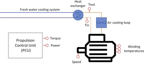
A schematic overview of the overall system we consider can be found in Figure 1. An on-board freshwater cooling system is used to control the temperature of the motor and other units. The motor itself is cooled by air, which is circulated by one or more fans. Heat is transferred from the hot air to the water-based cooling system through a heat exchanger, as seen in Figure 1. Cooling air temperature is measured on the inlet and outlet of the heat exchanger. The rotation speed of the motor is either measured directly, or provided by the Propulsion Control Unit (PCU), which is a controller application integrated with the propulsion frequency converter controlling the speed and power of the propulsion motors. The mechanical torque and electrical power are calculated and provided by the PCU. The system overview, shown in Figure 1, is fairly generic and will be suitable for other applications beyond electrical motors and diesel-electric propulsion systems on ships. More instrumentation may be available in some applications, but here a minimum set was chosen for training and implementation, in order for the protection function to be as general as possible.

Figure 1. Schematic overview of the system. The cooling air inlet and outlet temperatures are abbreviated Tin and Tout, respectively.

2. Data

2.1. Training data

The data made available by ABB consists of temperature and performance recordings from medium voltage (MV) electrical propulsion motors and the surrounding cooling system aboard four vessels of the same design. Each vessel has three different motors of two different classes, named class I and II in this paper, one motor of class I and two motors of class II. The temperature measurements (${}^{\circ }$C) on the windings of the motors were recorded by six sensors in total, located in two separate triplets of windings; referred to as $U_1,V_1,W_1$, and $U_2,V_2,W_2$. Several variables of the performance and the motor's surrounding cooling system could be measured, but the following subset of variables was recorded consistently across all the vessels: power of the motor (% of maximum nominal power), speed of the motor (% of maximum nominal speed), and mechanical torque (% of maximum nominal torque), together with the inlet temperature (${}^{\circ }$C), and the outlet temperature (${}^{\circ }$C) of the cooling air in the cooling system.

2.2. Preprocessing

The data from each vessel and motor was collected at different time periods in 2017 and 2018. The time periods of the collected data vary for the different vessels: 125 days, around 4 months, for the first vessel; 80 days, around 2.5 months, for the second vessel; 294 days, around 10 months, for the third vessel; and 262 days, around 9 months, for the fourth vessel.

The data was collected using the ABB Remote Diagnostics System (RDS), an edge device whose function is to collect data from the on-board devices and transfer it via a satellite link to cloud storage, enabling remote troubleshooting and data analysis. The on-board protection systems collect data at regular, sub-second intervals, while the RDS queries the data using different data collection schemes. In the considered training data, all measurements were collected using an asynchronous sampling regime. The idea behind the sample regime is that in order to not store more information than necessary, measurements are only recorded if they differ substantially from the previously measured value. Hence, values were polled at regular intervals, but only stored when the difference between the current and the previously stored value exceeded a given threshold. The threshold is configured differently for the different measurements. Under the asynchronous setup, substantial amounts of data are collected during dynamic periods, while none or few samples are recorded during stationary periods, for instance at zero power, e.g. docking, or when running at a constant power over a long period of time. The main strength of the asynchronous sampling regime is a reduction in storage capacity and bandwidth for data transfer during stationary periods, while still being able to record data with a relatively high bandwidth in dynamic periods (Losada et al. 2015). The main weakness is reduced robustness to data gaps, as missing measurements due to malfunctioning cannot be separated from stationary periods without additional information.

The temperature, performance, and cooling system measurements were thus recorded at non-uniform time intervals with gaps ranging from milliseconds to several hours or days. To obtain regularly sampled data, required for the machine learning analysis, all recordings were mapped onto a regular grid with 1 s sampling time, over the range spanned by the timestamps of all the measurements. The synchronisation of the temporal scale was applied to each ship separately as the collected data covered different periods. With several recordings within the same second, the last observed value was chosen.

To impute the non-recorded values in the regular time-aligned data, we applied a last value carried forward (LVCF) interpolation principle, separately for each variable. This complies with the asynchronous sampling regime in that a sequence of non-recorded measurements will be replaced by the last recorded value. Alternatively, given a synchronous sampling regime or a combination of asynchronous and synchronous measurements, a linear interpolation approach could have been used. There are, however, also indications of missing data due to malfunctioning registration. We therefore introduced a liberal upper threshold of 48 h for the length of the interpolation period, to avoid applying the LVCF principle to periods where it would clearly not be suitable. The value of 48 h was specifically chosen to not exclude certain long-distance voyages with stable conditions of high power observed in the data. A shorter upper threshold for the period length would have resulted in fewer observations in the time-aligned data necessary for the machine learning analysis. In addition, for the slowly changing temperature measurements, interpolation was only carried out if the difference between measurements at either end of the period was below 3${}^{\circ }$C. Changes in temperature larger than this threshold suggested that the missing observations were due to malfunctioning, and not the asynchronous sampling procedure. For the rapidly changing measurements, i.e. power, speed, and torque, a reasonable restriction could not be defined and interpolation was performed regardless of the change in value.

Before the synchronisation of the data, there were approximately 650,000 temperature measurements and 3 million observations for the power, speed, and torque measurements. After synchronisation, but before interpolation, there were around 450,000 complete observations with registered measurements in all variables. After the LVCF interpolation, there were around 78 million complete observations in the training data.

Finally, overheating can only occur when the motor is in fact running, and predicting the motor temperature at zero power corresponds to predicting ambient temperature. Therefore the final preprocessing step was to remove all observations where the power was approximately zero, set at the practical limit of the power being less than 1% of maximum nominal power.

3. Methods

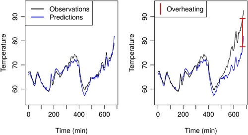
Our general framework for detecting heat development is to compare a prediction of the temperature in a normal state to the actually observed temperature, and to monitor deviations between the two. If the observed temperatures are significantly higher than the predicted temperatures, we may suspect overheating. The approach is illustrated in Figure 2. The left panel shows the observed and predicted temperatures under normal conditions, where they largely agree. The right panel, on the other hand, shows a hypothetical scenario where the observed temperature significantly exceeds the predicted temperature, indicating a possible overheating event. The novel contribution is to predict the winding temperature using a machine learning model to emulate the physical system. The prediction is based on available training data from the motor performance and cooling system under normal conditions, to describe how the temperature should behave.

Figure 2. Illustration of the general framework for overheating detection. The left panel shows the observed and predicted temperatures under normal conditions. The right panel shows an observed temperature significantly exceeding the predicted temperature, indicating a possible overheating event.

We therefore propose a two-step framework for overheating detection:

1. first, build a predictive machine learning model for the winding temperature based on observed historical data,

2. then, monitor and detect deviations in the observed winding temperatures from the predicted normal state values. When deviations exceed a certain threshold, an alarm is issued.

In the predictive step, we train the machine learning model to predict the mean motor temperature $T_m$ (averaged over all windings) to ensure generalisability as the locations of sensors and windings may differ across vessels and motors. In the detection step, we monitor the deviations of the observed temperature on the individual windings, in order to detect overheating events as early as possible. All analyses in the study were performed using the statistical software R.

3.1. Modelling temperature using machine learning

The first step is to train a machine learning model to emulate the physical system of the motor. We use ordinary least squares (OLS) linear regression (Chambers 1992; Friedman et al. 2001) as the machine learning algorithm, to comply with the practical constraints of the on-board protective system with limited computational power and memory. The OLS model predicts the mean motor temperature $T_m$, or the output $y_t$, at time t as a linear function of M input variables $x_{i,t}$ at time t: $y_t={\beta }_0+{\beta }_1{x}_{1,t}+\cdots +{\beta }_M{x}_{M,t}+{\epsilon }_t,$ with a noise term ${\epsilon }_t$. The initial input variables are the power, speed and torque of the motor and the cooling air inlet temperature. In addition, the cooling air outlet temperature is also available, but the role and subsequent exclusion of it from the considered model is discussed in Section 5.

The model is fitted by least squares using the QR factorisation method (Hansen et al. 2013). To optimise the predictive ability of the final model, we assess several reasonable transformations of the input variables and select the best in terms of prediction error.

3.1.1. Transformation of input variables

We first determine the relevant transformations of the input variables for the OLS regression algorithm. Expert knowledge regarding the physical system of the motor is used to guide the inclusion of relevant transformations. First, it is assumed that the impact of the motor speed and torque on the winding temperature would be the same irrespective of the direction of rotation, such that only the absolute values of the speed and torque variables are considered as inputs. The power of the motor is always positive.

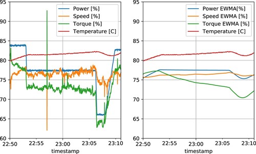
The motor performance measurements of speed, torque, and power are characterised by large and abrupt changes, as seen in the left panel of Figure 3. The individual sensor and mean temperatures are, on the other hand, slowly varying measurements as the motor, being a block of metal, heats up through conduction. We therefore consider time-lagged, smoothed transformations of the volatile input variables, as such smoothed variables will be more informative of the temperature, accounting for the time dynamics of the system. For our purpose, exponentially weighted moving average (EWMA) or exponential smoothing (Brown 1956; Holt 1957), is seen to be a good choice for constructing such lagged input variables. Importantly, exponential smoothing can be recursively defined, requiring minimal memory, such that the transformation is easily implementable in an industrial real-time system. Alternative smoothing approaches, such as fixed-window moving averages, would in comparison require more memory.

Figure 3. The left panel shows an example of abrupt changes in speed, power, and torque compared to the slowly changing mean temperature at an occurrence of acceleration of speed and torque. The right panel shows the corresponding exponentially smoothed variables of speed, power, and torque, together with the non-smoothed mean temperature.

EWMA smooths the time series using an exponential window function. It temporally lags the original input variable u by recursively adding current variable values to previous aggregates, multiplied by a smoothing factor $0<\theta <1$. More formally, the exponentially smoothed input variable, $x_t$ at time-step t, of the original input variable, $u_t$, is given by $x_t=(1-\theta )x_{t-1}+\theta u_t,u_0=x_0.$ The smoothing factor θ determines the time constant of the system, τ, where the relationship between θ, τ, and the sampling interval $\mathrm{\Delta }T$ is given by $\theta =1-e^{-\mathrm{\Delta }T/\tau }\simeq \frac{\mathrm{\Delta }T}{\tau },\tau \gg \mathrm{\Delta }T.$ The time constant, τ, of an exponential moving average is hence given by $\tau =\mathrm{\Delta }T/\log (1-\theta )$, and represents the amount of time it takes the smoothed response of a unit set function to reach 63.2% of the original signal. The EWMA characterises the solution to a first-order ordinary differential equation, and therefore gives a good approximation to physical systems such as heat transfer models.

When constructing the exponentially smoothed variables, a mechanism for handling the remaining missing or censored observations is needed. We choose to reset the exponential smoothing if an observation $x_k$ is missing or unavailable, meaning that the smoothing is initialised by setting $y_0$ equal to the first value after the missing observations. After a reset, the smoothing requires time to stabilise, such that the first 30 min are subsequently censored and not used.

3.1.2. Selection of input variables

We then select the best input variables to be included in the OLS algorithm. As prediction is our main aim, we evaluate the different models based on predictive ability using cross-validation. In cross-validation, different parts of the training data are consecutively held out from the model fitting and predicted based on the remaining data. The prediction error is then assessed by the root mean squared error (RMSE) averaged over all parts.

In our setting, the part of the training data held out could comprise either the data for one whole vessel, one motor class of a vessel, or one individual motor. Due to differing operating modes and varying sea conditions, the variability in motor operation between different vessels is substantially larger than the variability between motors within the same vessel. The two class II motors are, in addition, likely to run in the same mode within the same vessel. As we specifically aim to assess how the predictive performance generalises to a previously unobserved vessel, we perform cross-validation leaving out each vessel, i.e. the single class I motor and the pair of class II motors, in each cross-validation iteration. The cross-validation scheme therefore holds out all three motors in one vessel for each iteration. As the amount of available data varies between vessels, a weighted version of the root mean squared error is used. The vessel-specific weights equal the proportion of observations for each vessel of the total data, separately for the motor classes I and II. We further assume the physical systems of the class I and II motors to be equal, but that they may run under different operating regimes. The same input variables are therefore used for all motors, but with parameters estimated separately for the two motor classes.

We follow a forward and backward step-wise model selection strategy (Friedman et al. 2001), testing increasingly complex models and comparing them in terms of the cross-validated RMSE. The variables are included in the following hierarchy:

1. Cooling air inlet temperature

2. Linear power

3. Squared power

4. Linear speed

5. Squared speed

6. Linear torque

7. Squared torque

8. Interaction between linear speed, power and torque

All power, speed, and torque terms were included as exponentially smoothed variables as investigations showed that non-smoothed input variables always gave worse prediction performance. Details on the separate cross-validation errors for each step, when including different input variables, are provided in the Supplementary material. After a final backward step, excluding the variables not improving the prediction, the final model uses five input variables: cooling air inlet temperature, exponentially smoothed squared power, linear and squared speed, and squared torque.

As part of the model selection procedure, a conditionally optimal time constant, τ, was initially estimated separately for each input variable. To facilitate a physical interpretation of the model, all τ values were fixed to the same value, found to be $\tau =28\min$ by minimising the cross-validation RMSE. The model with a common time constant was seen to give only slightly worse prediction performance than the individual time constant model, see the Supplementary material for further details. The class I and II motor model fits are summarised in Table 1. We note that the sign of the estimated effect of the squared power differed between the models, which is likely due to the high correlations between the different input variables. The adjusted $R^2$ of the two models is 0.941 and 0.931, respectively. This close match between our predictive model and the observed data can be seen in the illustration in the left part of Figure 2. The training of the linear model with the training set of around 78 million observations runs in a couple of minutes on a standard computer.

Table 1. Estimated parameters for the temperature prediction models. The time constant τ is measured in minutes.

Variable	Class I motor	Class II motor
Constant	$2.7\cdot {10}^1$	$2.4\cdot {10}^1$
TaIn	$8.4\cdot {10}^{-1}$	$7.8\cdot {10}^{-1}$
Power${}^2$ ($\tau =28$)	$-3.5\cdot {10}^{-3}$	$1.0\cdot {10}^{-3}$
Speed ($\tau =28$)	$-4.0\cdot {10}^{-1}$	$-9.6\cdot {10}^{-2}$
Speed${}^2$ ($\tau =28$)	$5.7\cdot {10}^{-3}$	$2.2\cdot {10}^{-3}$
Torque${}^2$ ($\tau =28$)	$9.9\cdot {10}^{-3}$	$5.4\cdot {10}^{-3}$

3.2. Fault detection algorithm

Given the prediction models for the normal state of the system, the second step is to monitor the deviations between the observed temperature and the predicted temperatures. We propose an online monitoring algorithm for the temperature deviations based on the framework of Lorden and Pollak (2008) and Liu et al. (2017). We further develop a novel tuning procedure to automatically select the parameters of the monitoring algorithm.

The prediction models are trained on the mean temperature, but we monitor the observed temperature deviations on the individual sensors to detect overheating events as early as possible. For the fault detection algorithm, the aim is to detect as quickly as possible, whether any of the temperatures in N sensors suddenly rises to an abnormally high level compared to the normal state prediction. In our case, the number of sensors is equal to the number of individual windings, N = 6.

We use the notation $y_{j,t}$ for the observed temperature of the individual sensor $j=1,\dots ,N$ at time t, and ${\hat{y}}_t$ for the predicted average temperature across the sensors at time t produced by the models in Table 1. The deviations of the observed temperature from the predicted temperature at time t, referred to as the residuals, are given by $e_{j,t}=y_{j,t}-{\hat{y}}_t,j=1,\dots ,N.$ The goal is to detect whether the mean of the residual distribution for any of the sensors has changed sufficiently far from 0 in the positive direction. Such a large deviation is shown schematically in the right panel of Figure 2.

We monitor each sensor using a local monitoring statistic, $z_{j,t}$, which is a function of the temperature residuals of the jth sensor up until time t: $e_{j,1},\dots ,e_{j,t}$. We then construct a global monitoring statistic for all sensors, $G_t$, by applying a set of filtering or shrinkage functions, $h_j\ge 0$, on the local monitoring statistics of each sensor and summing their individual contributions, (1) $G_t=\sum _{j=1}^N{h}_j(z_{j,t}).$(1) Finally, the global monitoring statistic, $G_t$, is compared to an alarm threshold, b, where the alarm is raised when the statistic exceeds the threshold value.

The detection algorithm is required to detect true faults quickly with as few false alarms as possible and to detect faults that are only visible in a single sensor. At the same time, we need the algorithm to be computationally efficient and conceptually simple. Further, it should also generalise to different motors and vessels without motor-specific tuning. The simplicity of the monitoring system is important for the operator's understanding of the system and for implementation, as the monitoring system is coded in the on-board vessel system and must be able to run in real-time. We specifically select the local monitoring statistic $z_{j,t}$ and the filtering functions $h_j$ of the detection algorithm to comply with these criteria.

3.2.1. Choice of monitoring statistic

For the local monitoring statistic, we use the adaptive cumulative sum (CUSUM) statistic introduced by Lorden and Pollak (2008). We choose the adaptive CUSUM because of its simplicity and computational efficiency, in addition to a proven ability to quickly detect distributional changes of unknown magnitude. Alternative monitoring statistics include the standard CUSUM statistic (Page 1954, 1955), the EWMA control chart (Roberts 1959) or other sequential change-point detection statistics (Basseville and Nikiforov 1993).

We assume the residuals to be independent and standard normally distributed, such that the adaptive CUSUM statistic is given by (2) $z_{j,t}=max(z_{j,t-1}+{\hat{\mu }}_{j,t}{e}_{j,t}-\frac{1}{2}{\hat{\mu }}_{j,t}^2,0),$(2) for each sensor j. In practice, the overall distribution of the residuals in the training data is standardised to have a mean of 0 and a standard deviation of 1, separately for the two motor classes. The values ${\hat{\mu }}_{j,t}$ are adaptive means, recursively estimated for each sensor, given by (3) ${\hat{\mu }}_{j,t}=max(\frac{s_{j,t}}{n_{j,t}},\rho ),s_{j,t}=\{\begin{array}{ll}{s}_{j,t-1}+e_{j,t-1},& z_{j,t-1}>0,\\ 0,& z_{j,t-1}=0,\end{array}$(3) where $n_{j,t}=n_{j,t-1}+1$, if $z_{j,t-1}>0$, and otherwise $n_{j,t}=0$, if $z_{j,t-1}=0$, and with initial values $z_{j,0}=s_{j,0}=e_{j,0}=0$. Note that when $s_{j,t}=n_{j,t}=0$, we define $s_{j,t}/n_{j,t}=0$.

The adaptive means and the monitoring statistic $z_{j,t}$ are therefore dependent on a user-determined parameter, $\rho >0$, representing the smallest relevant change. If there is evidence that a change occurred, such that $z_{j,t-1}>0$, the mean is estimated by a recursively updated average. The update starts from a candidate change-point given by the most recent time i where $z_{j,i}=0$ for $1\le i\le t-2$. If there is no evidence of a change, such that $z_{j,t-1}=0$, the average is reset to 0. The statistic will further ignore irrelevant changes when ρ is selected appropriately. When the monitoring statistic is zero, $z_{j,t-1}=0$, the consecutive value only increases, $z_{j,t}>0$, if $e_{j,t}>\rho /2$. At a given observation time t, the number of operations needed to update the monitoring statistic is independent of both the training set's size as well as the length of the current monitoring period, t. The computational complexity scales only linearly in the number of sensors N (i.e. $O(N)$). The required calculations in real-time are thus very limited and run on the scale of milliseconds, even if there are thousands of sensors.

The assumed normality and independence of the residuals is, however, an oversimplification and results in a misspecified model. But due to the large amounts of available training data and the fact that the temperature faults of interest correspond to large changes in the mean, this simplistic model still yields good results in practice. Further, the threshold b is set based on the number of false alarms in the training data, irrespective of the model assumption of the CUSUM statistic. The model misspecification therefore does not result in loss of control of the false alarms, but rather speed of detection. Given that the relevant changes in the means are relatively large, any improvement in timeliness achieved by applying a more complex residual model appears to be small.

In the standard CUSUM, changes in the mean have to be pre-specified. The recursive estimation of the mean in the adaptive CUSUM makes this approach more flexible. The adaptive CUSUM is therefore less prone to degrading performance due to a misspecified μ compared to the standard CUSUM, and it achieves two goals simultaneously: ρ may be specified at the lowest possible level to filter out all small, non-relevant changes, while at the same time maintaining near optimal detection speed for changes of mean greater than ρ. This point is further discussed in Section 3.2.3. This feature is important when only one fault is available for testing, as new faults will be different in terms of the size of the change in mean. In the standard CUSUM, μ must be balanced between these two goals, not being optimal for any of them. The standard CUSUM is also prone to overfitting μ to the observed fault, suggesting that the adaptive CUSUM generalises better to other vessels and faults.

3.2.2. Choice of global monitoring statistic

For the global monitoring statistic, we use the maximum over all sensors (4) $G_t=\underset{j}{max}(z_{j,t}),j=1,\dots ,N,$(4) which is given by the order-thresholding filtering function, $h(z)=z\mathbf{1}\{z\ge z_{(1)}\}$, where $z_{(1)}$, the largest order statistic, is the maximum of $z_1,\dots ,z_N$. The order-thresholding applied to the sum in Equation (1(1) $G_t=\sum _{j=1}^N{h}_j(z_{j,t}).$(1) ) truncates the terms not corresponding to the maximum to zero. Alternative filtering functions such as hard- and soft-thresholding, $h(z)=z\mathbf{1}\{z\ge a\}$ and $h(z)=max(z-a,0)$, depend on an additional constant a.

The maximum function is chosen to allow for quick detection of faults affecting only a single sensor, i.e. emerging hotspots, as it is known to be more efficient than the sum or average of sensors for such faults (Mei 2010; Xie and Siegmund 2013; Liu et al. 2017). Soft- or hard-thresholding may yield faster detection speed for faults affecting all sensors (Liu et al. 2017), but as the max filtering does not introduce additional tuning parameters, it allows for better generalisability to new and previously unobserved vessels. The fault detection algorithm is summarised in Algorithm 1.

3.2.3. Setting the detection threshold and minimum change size

To apply the detection algorithm in practice, we are required to determine the detection threshold, b, and the minimum change size, ρ. These parameters are tuned to detect a fault as early as possible, while controlling the number of false alarms, and at the same time setting ρ as low as possible without severely compromising the detection speed. The latter counteracts overfitting due to the limited number of faults, only one single incident, and can therefore improve generalisability. The detection threshold, b, is set relative to the number of acceptable false alarms, m, in the fault-free training data. We define a potential false alarm event as the contiguous time-points where the statistic $G_t$ raises above 0 for a certain period of time, before going back to 0 again. What governs the threshold b is the maximum value of $G_t$ in each such region. To be precise, if $I_j$ for $j=1,\dots ,k$ denote the k potential false alarm events in the training data, then the value of $G_t$ at the peak over each interval is given by ${\hat{G}}_j=\underset{i\in I_j}{max}{G}_i$. A threshold can then be obtained by setting b to the $(m+1)$th largest ${\hat{G}}_j$. As the threshold depends on both ρ and m, we use the notation $b(\rho ,m)$ when it is useful to make this dependence explicit.

The time of an alarm corresponds to the first time the monitoring statistic exceeds the threshold, denoted as a function of ρ and m by $A(\rho ,m)=min\{t\ge 1:G_t>b(\rho ,m)\}.$ Given that F is the time of a true fault, detecting the fault as early as possible while allowing m false alarms, can be formulated as maximising $T(\rho ,m)=F-A(\rho ,m),$ with respect to ρ for a given m. As multiple values of ρ and corresponding thresholds $b(\rho ,m)$ may achieve approximately the same time to failure T, we select the smallest ρ maximising T within a user-specified error margin δ: $\hat{\rho }(m)=min\{\rho >0:\underset{\rho >0}{max}\{T(\rho ,m)\}-T(\rho ,m)\le \delta \}.$ The corresponding threshold for a specific number of false alarms m is then given by $b(\hat{\rho },m)$. A grid search over ρ was used to find an approximately optimal $\hat{\rho }$. Given a training set of size n, the computational complexity to tune the penalty for a fixed ρ and m is $O(nN)$. Hence, for a given number of false alarms, m, the number of operations is $O(nN)$ times the size of the grid over ρ in the grid search.

The error margin δ is introduced to reduce overfitting of ρ to the one single fault. We experienced that an error margin of 1 s resulted in ρ being set too high for possible future faults, because a slightly higher ρ resulted in a few seconds quicker detection. With δ, one can specify, for example, that all detection times within 60 s of the optimal detection time are good enough. We found that a δ of three minutes provided a decent counter-balance to maximally overfitting ρ to our single fault case presented in the next section.

4. Performance on real failure case

In this section, we present the results of the detection algorithm (Algorithm 1) applied to a real overheating failure case. The failure occurred in one of the vessels available in the training data, following the system described in Section 1.1, but outside the training period. For this specific failure event, the inhibit alarm (HH) at ${155}^{\circ }$C was never reached and triggered, as the system was damaged below the hard threshold. The upper panel of Figure 4 shows the residuals of the N = 6 temperature sensors in the four hour period before the motor fails. The lower panel of Figure 4 shows in the same period the corresponding individual CUSUM statistics (gray lines) and the maximised adaptive CUSUM statistic (black line) following Algorithm 1. Only the top two largest individual CUSUM statistics are visible in the figure. The displayed CUSUMs use $\rho =17.8$, which is the optimal ρ for m = 0 false alarms in the training data, obtained by the procedure described in Section 3.2.3. The time of the motor failure is indicated by the red line. The missing values in the residuals and the CUSUM statistic are due to the motor being shut off, resulting in zero power, and the subsequent initialisation of the exponentially smoothed variables, requiring a 30 min burn-in period. The tuning of the monitoring parameters was completed in about four and a half hours (3.6 min for each value of $\rho =5,5.2,\dots ,20$.).

Figure 4. (a) The residuals of each of the six temperature sensors before the fault. (b) The corresponding adaptive CUSUM statistics per sensor $z_{j,t}$ (gray lines) and their maximum $G_t$ (black lines), for $\hat{\rho }=17.8$ for zero false alarms (m = 0) found by the procedure described in Section 3.2.3. The trained detection threshold for these values of $\hat{\rho }$ and m is b = 2170, and it gives an earliest possible detection time (green dashed vertical line) of 57 min prior to the fault.

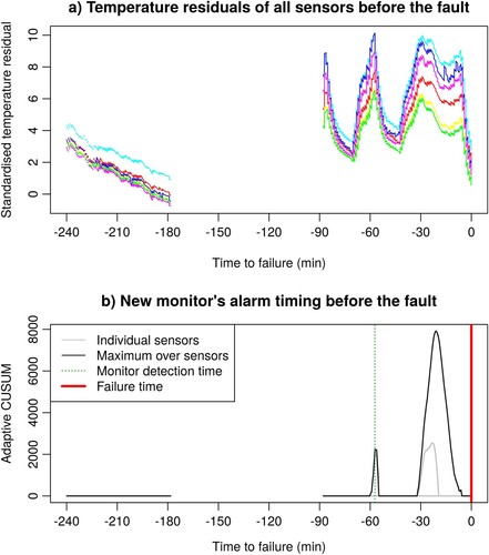
If no false alarms are allowed in the training period, the fault is detected as early as 57 min (vertical green dashed line) before the motor failure. The alarm is raised when the mean temperature is 104.2${}^{\circ }$C and the maximum temperature over the six sensors is 111.3${}^{\circ }$C. By allowing for one or two false alarm events in the training period, the detection time remains approximately the same (around 56 min), but ρ may be lowered to 16.2 and 12.4, respectively, following the tuning strategy in Section 3.2.3. The lower ρ values improve the generalisability of the monitoring algorithm to new faults. Finally, if we allow for three false alarms in the training period, the fault may be detected already at 86 min prior to the failure, with a value of $\rho =17.2$. The alarm is then raised when the mean temperature is 91.0${}^{\circ }$C and the maximum temperature over the six sensors is 98.3${}^{\circ }$C. Further allowing for four to ten false alarms in the training period did not improve the detection time, but lowered the optimal ρ value.

5. Discussion

We have demonstrated how a data-driven approach of using past data and machine learning can provide timely prediction of overheating in marine vessels. The overall procedure is designed for a real-time setting, with minimal requirements for memory and computational power, such that it may run on any on-board control system. Based on assessing a real failure case, our proposed alarm algorithm may detect a fault between 60 and 90 min before the actual occurrence and at temperatures below the current alarm limits, depending on the permitted number of false alarms in the training data. By using a machine learning approach, one can capture predictive relationships, interactions or feedback-loops, that may be unknown or non-intuitive to experts of the physical model. Physical knowledge was only included in the model building step to guide the selection and transformation of candidate input variables considered by the model. Note that we do not aim to replace existing hard-threshold prevention standards, but we believe data-informed tools will become an important and timely supplement.

The aim of this work was to use data from a subset of four vessels to create two models (class I and II) that could be used on all vessels in the fleet. The model was hence trained on the average winding temperature, while the monitoring algorithm itself was implemented on each individual winding. It should therefore be noted that better performance could probably be obtained by training winding-specific models. For all motors, the winding temperatures had a variation of around 3–4${}^{\circ }$C, which appears to be consistent for each motor, but no pattern could be found across motors. The bias is, therefore, likely caused by installation or manufacturing effects, and individual models for each winding would be able to filter out these biases and hence improve the monitor performance. However, as these differences are motor-specific, this would require retraining of the model for each new vessel.

A drawback of the model-based approach is that data is needed to build the models for a specific cooling system configuration and motor type. Data is needed both for building machine learning models, and for parameter identification in the case of a physics-based model. Since only existing instrumentation is utilised, there is no additional cost (for instance for purchasing or installing sensors) associated with the approach. The model cannot be implemented on a new configuration directly. However, we believe that the selection of parameters and methodology could be applicable to systems similar to this particular class of identical vessels.

Based on a single fault, it may be difficult to assess how the probability of detection and the detection time will generalise to other overheating events. Further assessments of the procedure is therefore needed, both on more vessels and faults. The difficulty of obtaining failure cases stems both from the fact that they are rare (as a number of protections are in place to avoid overheating of the motor due to the extreme adverse consequences) and not openly available (as no similar incidents are known in any open literature or published data sets). Importantly, both a larger number and a wider range of faults should be used to validate how well the detection framework generalises beyond the current fault case. If a substantial number of fault cases can be obtained, machine learning models may also be applied directly to predict alarms, instead of monitoring the deviation from the normal state. Additional fault cases may also improve the estimates of the probability of detection and the timeliness of our procedure.

For the prediction of the motor temperature, there were several models, or combinations of input variables, that gave similar or identical prediction performance. It is reasonable to expect that the exact ordering of the different models would change if more data was included. Also, the final model is likely to depend on the order of which the input variables were included. Hence, there may be no one single preferred model, clearly outperforming and superior to the rest. However, we aimed to select the final model consistently by including the input variables lowering the prediction error, while ensuring a parsimonious model.

In addition, it should be noted that including the air outlet temperature of the cooling system in the model would lower the prediction error (in terms of RMSE) by around a factor of one half. The air outlet temperature is strongly correlated with the winding temperatures, and hence has a high predictive power. But the causal relation between the two is known to be misleading for our final aim, as it is the motor temperature that causally affects the air outlet temperature. Any anomalous increase in winding temperature will after a while lead to an increase in the air outlet temperature. Our detection algorithm relies on observing a deviation from the prediction of the normal state. However, under any system state, either normal or faulty, one would expect the same relation between the motor temperature and the air outlet temperature. Thus, if we include the air outlet temperature, there is a risk of the motor temperature being well predicted (due to the air outlet temperature) even during instances of overheating. And as the main aim is to detect deviating observed temperatures as early as possible, including the air outlet temperature inherently introduces a risk of masking overheating cases.

More complex machine learning approaches may also be utilised in the prediction step. This could include recurrent neural network and deep learning, such as the popular Long Short Term Memory (LSTM) models or Gated Recurrent Units (Hochreiter and Schmidhuber 1997; Cho et al. 2014). These methods, however, require excessive computational time and memory not available at the current on-board system implementation. Future work needs to assess whether such complex algorithms may improve the predictive performance in the initial modelling step of our framework.

Acknowledgments

The authors would like to thank Bo-Won Lee and Jaroslaw Nowak at ABB Norway for valuable support in the development of this project.

Disclosure statement

No potential conflict of interest was reported by the author(s).

Additional information

Funding

This work was supported by Norwegian Research Council centre Big Insight project 237718.

Notes on contributors

K. H. Hellton

K. H. Hellton is a Senior Research Scientist at the department of Statistical analysis, machine learning and image analysis (SAMBA), Norwegian Computing Center, with an expertise in high-dimensional statistical methods. He has worked on several projects in predictive maintenance, applying statistical methods and machine learning to sensor data.

M. Tveten

M. Tveten is a Research Scientist at the Department of Statistical analysis, machine learning and image analysis (SAMBA), Norwegian Computing Center, and former PhD student at the Department of Mathematics (Statistics and Data Science research group), University of Oslo, specialising in statistical anomaly and change detection.

M. Stakkeland

M. Stakkeland works with analytics and data science in ABB Marine and Ports. He has a leading role in developing new digital solutions and analysing operational data from equipment and systems onboard ships. He has a position as Associate Professor II at the Department of Mathematics (Statistics and Data Science research group), University of Oslo.

S. Engebretsen

S. Engebretsen is a Research Scientist at the Department of Statistical analysis, machine learning and image analysis (SAMBA), Norwegian Computing Center. She works with statistical modelling and machine learning with different application, for instance infectious disease modelling and sea lice control. She has interests in statistical methods for high-dimensional data, statistical prediction and inference.

O. Haug

O. Haug is a Senior Research Scientist at the Department of Statistical analysis, machine learning and image analysis (SAMBA), Norwegian Computing Center, with a proficiency in regression models, time series analysis and extreme value statistics. His experience includes assessing and modelling sparse sensor data in projects for the maritime and transport industry, and he also has a background in oceanographic consultancy.

M. Aldrin

M. Aldrin is Chief Research Scientist at the Department of Statistical analysis, machine learning and image analysis (SAMBA), Norwegian Computing Center, with an expertise in statistical modelling. He has worked within a variety of research fields including climate modelling, fishery and aquaculture, health and transport.

References

- Basseville M, Nikiforov IV. 1993. Detection of abrupt changes: theory and application. Englewood Cliffs: Prentice Hall.
- Brown RG. 1956. Exponential smoothing for predicting demand. Cambridge (MA): Arthur D. Little Inc.
- Chambers JM. 1992. Chapter 2 Linear models. In: Chambers JM, Hastie TJ, editors. Statistical models in S. Boca Raton, Florida: Chapman & Hall/CRC.
- Cho K, Van Merrienboer B, Gulcehre C, Bahdanau D, Bougares F, Schwenk H, Bengio Y. 2014. Learning phrase representations using RNN encoder-decoder for statistical machine translation. In: Proceedings of the Conference on Empirical Methods in Natural Language Processing (EMNLP 2014), Doha, Qatar.
- Friedman J, Hastie T, Tibshirani R. 2001. The elements of statistical learning: data mining, inference, and prediction. Vol. 1, No. 10. New York City (NY): Springer.
- Gnacinski P. 2008. Prediction of windings temperature rise in induction motors supplied with distorted voltage. Energy Convers Manag. 49(4):707–717.
- Hansen PC, Pereyra V, Scherer G. 2013. Least squares data fitting with applications. Baltimore, Maryland: JHU Press.
- Hochreiter S, Schmidhuber J. 1997. Long short-term memory. Neural Comput. 9(8):1735–1780.
- Holt CC. 1957. Forecasting trends and seasonal by exponentially weighted averages. Vol. 52. Office of Naval Research Memorandum.
- IEEE Standard 3004.8. 2016. Recommended practice for motor protection in industrial and commercial power systems. New York City (NY): IEEE.
- Liu K, Zhang R, Mei Y. 2017. Scalable SUM-shrinkage schemes for distributed monitoring large-scale data streams. Stat Sin. 29:1–22.
- Lorden G, Pollak M. 2008. Sequential change-point detection procedures that are nearly optimal and computationally simple. Seq Anal. 27(4):476–512.
- Losada MG, Rubio FR, Bencomo SD, editors. 2015. Asynchronous control for networked systems. Heidelberg: Springer.
- Lystianingrum V, Hredzak B, Agelidis VG. 2016. Multiple-model-based overheating detection in a supercapacitors string. IEEE Trans Energy Convers. 31(4):1413–1422.
- Maftei C, Moreira L, Guedes Soares C. 2009. Simulation of the dynamics of a marine diesel engine. J Mar Eng Technol. 8:29–43.
- Mei Y. 2010. Efficient scalable schemes for monitoring a large number of data streams. Biometrika. 97(2):419–433.
- Page ES. 1954. Continuous inspection schemes. Biometrika. 41:100–115.
- Page ES. 1955. A test for a change in a parameter occurring at an unknown point. Biometrika. 42:523–527.
- Pawlus W, Birkeland JT, Van Khang H, Hansen MR. 2017. Identification and experimental validation of an induction motor thermal model for improved drivetrain design. IEEE Trans Ind Appl. 53(5):4288–4297.
- Roberts SW. 1959. Control chart tests based on geometric moving averages. Technometrics. 1:239–250.
- Vanem E, Brandsæter A. 2019. Unsupervised anomaly detection based on clustering methods and sensor data on a marine diesel engine. Journal of Marine Engineering & Technology.
- Xie Y, Siegmund D. 2013. Sequential multi-sensor change-point detection. Ann Statist. 41(2):670–692.