Quay-to-quay mission with autonomous docking: a model-scale experimental validation

Abstract

Transport of cargo by short-sea shipping is at the forefront of the European Union's transportation policy. It has the promise to alleviate congested land transport and decrease pollution [European Commission. 2021. Putting European transport on track for the future]. However, the shortage of qualified personnel might impede this solution. Autonomous sailing of ships could help, especially if the whole trip is automated. In this study a control system is designed that is capable of sailing a round-trip with a model-scale feeder vessel in Marin's Seakeeping and Manoeuvring Basin. The Guidance-Navigation-Control framework is used to sail this journey with attention given to smooth switching between the operational modes. A set of experiments is conducted to validate the controller and identify crucial parts in the operation. The experiments showed that the controlled vessel can sail a round-trip with different levels of waves and wind disturbances coming from different directions. Furthermore, the round-trip can be modified such that the approach angle to the quay changes and the ship still successfully docks at the quay. It was found that the approach to the quay is most difficult during transition from high to low speed, when the bow thrusters have yet to become effective, and a large change in course is needed. This can be circumvented by changing the trajectory to the quay to have a longer straight approach, or it can be corrected when the bow thrusters become active.

Keywords:

• Maritime Autonomous Surface Ship (mass)
• Guidance – Navigation - Control
• Autonomous docking
• Model-scale experiment

1. Introduction

The maximum number of containers carried by deep sea container ships increases steadily over time. At the time of writing this number almost reaches 25 000 teu. As a result, smaller ports, for example in the Mediterranean Sea, cannot harbour these ships. Transport over land, if possible, is often congested. Smaller feeder vessels, with a capacity below 3000 teu and an average capacity between 300 and 1000 teu, can distribute the cargo from deep sea container vessels to these smaller ports. However, this solution is impeded by the shortage of qualified personnel. In this situation, autonomous sailing of feeder vessels to these smaller ports would help. To provide a real advantage, the whole trip should be automated. Improving the short sea shipping services was a subject of the eu-h2020 Moses project where autonomous sailing between ports is one of the tasks (De Juan et al. 2022).

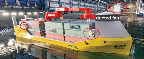
The aim of this work is to design a control system capable of sailing from one quay to the next, including the (un)docking phase, with an 1:17 model-scale feeder vessel in Marin's Seakeeping and Manoeuvring Basin (smb). Experiments are done to validate the control system and to identify crucial parts in the operation. The solution is tailored to a 71 m long feeder vessel previously designed in the project. A picture of the feeder vessel in the smb is shown in Figure 1. Due to space limitations in the smb, the departure and arrival quay are the same. The term round-trip is therefore used.

Figure 1. 1:17 scale model of the container feeder vessel in Marin's Seakeeping and Manoeuvring Basin. Ducted fans to generate wind disturbances are encircled.

The round-trip is divided into several phases. The first split is made into ‘undock’, ‘transit’ and ‘dock’ (Walmsness et al. 2023). During the undock phase, the vessel leaves the quay slowly and, once at a safe position from the quay, it switches to the transit phase. The ship transits to the other harbour by tracking a set of waypoints. When it reaches the harbour, the vessel has to dock at the quay. This part of the operation is again divided into an ‘approach’ phase, partially executed under-actuated and partially executed fully-actuated, and a dock phase (Okazaki and Ohtsu 2008; Ahmed and Hasegawa 2015). The change from under-actuated to fully-actuated is introduced because the bow tunnel thrusters become available at low speed. The operational phases have to be combined to sail the full mission. The commands to the actuators should not alter discontinuously at these switches, as argued in Alessandri et al. (2019); Walmsness et al. (2023). The experiments are performed with the assumption that there is no manoeuvring needed in the port, although such an operational state could be added. Furthermore, there are no other ships or unknown obstacles included.

The vessels dynamic behaviour, the efficiency of the actuators, as well as the requirements, all change depending on the phases of the mission. Therefore, the control strategy changes depending on which phase the operation is in. For each of the phases, the Guidance-Navigation-Control (gnc) framework is used (Shneydor 1998). In this scheme, the guidance provides setpoints to the vehicle controller such that the route of the vessel coincides with that of a (moving) target, and hence the vessel can track the desired route. In the transit phase, the system is under-actuated and a Line-of-Sight (los) guidance law (Breivik 2010; Lekkas and Fossen 2012) is used to provide a speed and a heading setpoint to the autopilot (Neuffer and Owens 1992; Fossen TI 2021). At low speeds, such as in the (un)docking phase, all degrees of freedom can be controlled independently, and the guidance can directly provide the setpoints to the vehicle controller. This closely relates to a dp system (Sørensen 2011).

Approaching the quay is the most difficult part in the operation, as the speed and the course change simultaneously. The approach phase for commercial ships has received much attention over the last decades. One method is to treat it as an Optimal Control Problem (ocp) for which the trajectory and the actuator settings are calculated at the start of the approach phase (Djouani and Hamam 1995; Ohtsu et al. 1996; Okazaki and Ohtsu 2008; Miyauchi et al. 2022), or repeatedly at each sample time (Mizuno et al. 2015; Martinsen et al. 2019; Bitar et al. 2020; Li et al. 2020). Another method is to learn the control based on the actions of a real captain, or to deduce it from a model (Hasegawa and Kitera 1993; Ahmed and Hasegawa 2015; Im and Nguyen 2018; Shuai et al. 2019; Mizuno and Koide 2023). In these methods the guidance and the control are combined. In order to better show the personnel what is happening, as done with a manoeuvring assistant in Schubert et al. (2019), the vehicle control and the guidance can be separated. The gnc framework for the approach phase is also found in Piao et al. (2019); Schubert et al. (2019); Sawada et al. (2021). Literature reviews on the automatic docking problem are provided by Qiang et al. (2022),Lexau et al. (2023),Zhang et al. (2023). As indicated before, the approach employed in this work is the gnc framework. It allows a clear separation of functions, and it allows to modularly change a single component while retaining the other components.

The contribution of this work lies in a set of experiments where the vessel sails a full trip from one quay to the next. Similar results are not found in the above-cited references. Our experiments systematically test the control approach designed for a model-scale vessel for different disturbances. The disturbances levels tested are such that the real disturbances do not exceed these with 30%, 50% and 70% probability at the port of Mykonos.

A further contribution is the gnc framework for the approach phase which combines a Bézier trajectory with a Constant Bearing (cb) guidance law. This provides continuous setpoints and derivatives thereof to the vehicle controller, such that this controller can be designed as a linear controller. This work consolidates work previously presented in de Kruif (2022a), de Kruif (2022b), de Kruif (2023), de Kruif (2024), Daalen et al. (2023), de Kruif et al. 2023).

This article starts with a description of the operation that we want to execute and a decomposition thereof in Section 2. The switching mechanism employed will also be treated in this section. The controllers use a dynamical model of the feeder vessel. The vessel and its dynamic behaviour are treated in Section 3. In this section a detailed simulation model is introduced, from which simplified control models are deduced, used to design the controllers with. Section 4 treats the guidance and the vehicle controller of each phase. The allocation algorithm that relates the force required from the vehicle controller to the active thrusters also needs to switch depending on the phase of the operation. The allocation algorithm is treated in Section 4. In Section 5, we present the experimental set-up and the results. Section 6 presents the conclusions.

2. Quay-to-quay mission

2.1. Description of phases

Figure 2 shows the mission considered. The corresponding state diagram, indicating which guidance, control and allocation algorithms are active is shown in Figure 3. The following operational states are distinguished:

Figure 2. Decomposition of a simple quay-to-quay mission where the departure quay and the arrival quay are the same. The dots in the transit phase denote the waypoints. The vessel is shifted between the dock and undock phase for visual clarification.

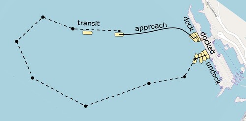
Figure 3. Mission state diagram. Each state has its own guidance (G), controller (C) and allocator (A), which are treated in more detail in Section 4. The approach phase is split in an under-actuated (UA) part and a fully-actuated (FA) part.

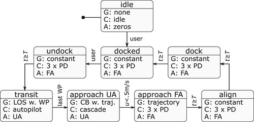
1. docked: The vessel is docked at the quay. A pose just behind the quay is provided as setpoint to the controller. The vessel will continuously push against the fenders to try to reach this pose. Three independent Proportional-Derivative (pd) controllers are used to control each degree of freedom. The vessel will start undocking on the user's mark.

2. undock: The vessel moves away from the quay and orientates itself such that its heading points towards the first waypoint. The distance from the dock is provided by the user. All motions are slow, which again allows for three independent pd controllers. After a specified time when the pose is reached, the transit phase is initiated.

3. transit: The vessel sails a track pre-defined by a set of waypoints at cruising speed. A los guidance law is used to convert the track between the waypoints to a velocity and a heading setpoint. An autopilot is designed to sail this track with only the stern azimuthing thrusters. Once the last waypoint is passed, the approach phase is started.

4. approach: In the approach phase, the vessel decelerates from cruising speed to a stand-still at a pre-defined safe pose close to the quay. The vessel must follow a smooth trajectory connecting these poses. The first part of the approach phase is done in the under-actuated mode. When the speed drops below u= 0.5 m/s, the bow tunnel thrusters become available and the pose can be forwarded directly to three independent pd controllers. When the approach trajectory is completed, the docking phase is initiated.

5. docking: In this final phase, the fully-actuated vessel slowly moves sideways from the safe pose to the quay.

The ‘idle’ phase in Figure 3 is not so much an operational phase, but a convenience way to start the experiments. Nothing is done: it allows us to inspect if everything is working as intended.

2.2. Mission execution

Now that the mission has been reduced to a sequence of phases, the state machine can execute the mission. Each phase has a specific control strategy or ‘controller’ and a specific allocation strategy or ‘allocator’. Depending on the vessel state and pre-defined conditions, the state machine switches to the next phase. To avoid jumps in the switching, information is passed on to the next controller and a smooth switching scheme has been employed that is further treated in Section 4.4.

3. Ship motion model

The main particulars of the full-scale vessel are given in Table 1. The vessel has two stern azimuthing thrusters for main propulsion and two bow tunnel thrusters for assistance at low speed manoeuvring. A dynamic model is used to design our controllers. Not only the feedback controller is based on these models, but the a-priory knowledge is also used to create a feedforward controller with.

Table 1. Main particulars of container feeder vessel.

description	symbol	value	unit
length	$L_{\mathrm{pp}}$	71	m
beam	B	13	m
mean draft	$T_{\mathrm{m}}$	4.5	m
displacement volume	∇	2899	m${}^3$
total mass in surge direction	$m_x$	$3.19{10}^6$	kg
total mass in sway direction	$m_y$	$4.57{10}^6$	kg
total inertia in yaw direction	$I_z$	$1.36{10}^9$	kgm${}^2$

Note: Total mass indicates the sum of rigid body mass and added mass. An 1:17 scale model is used in the experiments.

3.1. Detailed simulation model

A detailed simulation model is available to construct the simplified dynamic models. The model is assumed to be given and is treated in more detail in Daalen et al. (2023). The elements included are

• Hydrostatic forces, calculated from the 3D hull shape. These forces are linearised around the hydrostatic equilibrium since we operate at small roll and pitch angles.

• Hydrodynamic forces: calm water resistance and manoeuvring forces. These are first calculated by means of cfd computations, and then approximated by a set of resistance and manoeuvring coefficients for time-domain simulations.

• Wave radiation forces, included as frequency-dependent-added mass and damping coefficients.

• Wave excitation forces, calculated by linear diffraction theory. Both first-and second-order wave forces are included.

• Four-quadrant propeller characteristics for the stern and bow thrusters are used to calculate the thrust and torque generated from the rpm.

The equations of motion are solved for all six coupled degrees of freedom.

3.2. Simplified control models

Three different controllers are used, as shown in Figure 3. Control models that describe the dominant dynamics are used to design these controllers. The independent pd controllers assume that the speed is low and all degrees of freedom are uncoupled. The autopilot and the cascade controller assume that the heading and the speed are decoupled. As long as both variables change sufficiently slow and are individually controlled tightly enough, the interaction is limited. A relation between course and heading is also determined in order to sail a course over ground with a heading controller.

3.2.1. Zero-speed control model

At near-zero speed, the dominant dynamics can be described by a moving mass. The transfer function for a moving mass relating force to position is given as $x/F=1/$(ms${}^2)$, where s indicates the Laplace variable and m can be one of the total masses $m_x,m_y$ or $I_z$ as given in Table 1. The values of these masses are part of the detailed simulation model and are directly used. The force has to be applied at the cog to avoid coupling between the degrees-of-freedom.

3.2.2. Forward speed control model

The manoeuvring model for forward speed, with the hydrodynamic cross-coupling removed, is given as: (1) $m_x\dot{u}=m_x\mathrm{vr}+X_{u|u|}u|u|+F_x,$(1) where $m_x$ is the total body mass, $X_{u|u|}$ the quadratic surge damping coefficient fitted to the cfd data, and u, v, r are the velocities in surge, sway and yaw direction. $F_x$ denotes the surge force and is applied in line with the cog. The parameter values are given in Table 2.

Table 2. Parameter values identified for the three parts of the control model.

Model	Parameter	pole/zero
speed	$m_x=3.19{10}^6$ kg
	$X_{u|u|}=-1506$ kg/m
rate-of-	$\alpha =-8.47{10}^5\cdot u$	$p=9.27{10}^{-3}\cdot u$
turn	$\beta =4.84{10}^9/u$
	$K/T=1.09{10}^{-8}$
course	$a=9.784{10}^{-3}\cdot u$	$p=-9.78{10}^{-3}\cdot u$
	b = −0.512	$z_1=-7.62{10}^{-3}\cdot u$
	$c=-10.1/u$	$z_2=3.19{10}^{-2}\cdot u$

Note: The right-most column lists the poles and zeros for the linearised transfer function around zero. u indicates the surge velocity.

3.2.3. Rate-of-turn/heading control model

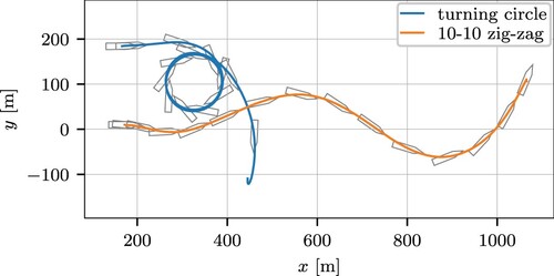
The vessel is course unstable as shown in Figure 4: After the turning circle the rate-of-turn does not return to zero, and the amplitude of a 10-10 zig-zag keeps increasing. This behaviour is described by a first order Nomoto model (Neuffer and Owens 1992): (2) $\dot{r}=-\frac{K}{T}(\alpha +\beta r^2)r+\frac{K}{T}{F}_y.$(2) Here, the rudder angle has been replaced by the sway force $F_y$, applied at the location of the azimuthing thrusters. In this equation r denotes the rate-of-turn, and $\alpha <0,\beta >0,K/T>0$ are parameters to be determined. The values of $\alpha ,\beta$ are found by fitting them on a Bech's reverse spiral, while the value of K/T is found by the step response around the $F_y=0$ equilibrium.

Figure 4. The path of the feeder vessel for a turning circle and 10-10 zig-zag test.

The linearised transfer function of (2(2) $\dot{r}=-\frac{K}{T}(\alpha +\beta r^2)r+\frac{K}{T}{F}_y.$(2) ) at r = 0 is calculated as follows: (3) $\frac{r}{F_y}=\frac{K/T}{s+\mathrm{\alpha K}/T}\to \frac{\psi }{F_y}=\frac{K/T}{s(s+\mathrm{\alpha K}/T)}.$(3) where ψ denotes the heading. The pole corresponding to the linearised system is given in Table 2 and the positive sign shows the unstable behaviour of the system at this operating point. The location of the pole changes to the left-half plane if we linearise around an increased rate-of-turn.

3.2.4. Course control model

The relation between the course and the heading is based on Yu et al. (2008): (4) $\dot{\chi }=-a\chi +a\psi +(1+b)\dot{\psi }+c\ddot{\psi },$(4) in which χ denotes the course, and a, b, c are parameters. In Yu et al. (2008) the parameter c is not present. However, if a lateral force is applied, the vessel will move to the side first, and only when it has rotated, then the surge speed will change the course to the other direction. At lower speeds, this effect is significant. This non-minimum phase behaviour is caught if $c\ne 0$, and is illustrated in Figure 5.

Figure 5. The course χ and rate-of-turn r with fixed surge speed u = 0.5 m/s and a step of $r_{\mathrm{sp}}=0.1$ deg/s on the reference rate-of-turn.

The course and rate-of-turn with fixed surge speed and a step on the rate-of-turn setpoint.

The parameters values were identified in a closed-loop simulation in which the rate-of-turn was controlled. The rate-of-turn setpoint was changed stepwise. By means of a least-squares fit the relation between the drift angle and rate-of-turn in (4(4) $\dot{\chi }=-a\chi +a\psi +(1+b)\dot{\psi }+c\ddot{\psi },$(4) ) was calculated. The values are given in Table 2. The transfer function is: (5) $\frac{\chi }{\psi }=\frac{c{s}^2+(1+b)s+a}{s+a}=\frac{({\tau }_{z_1}s+1)({\tau }_{z_2}s+1)}{{\tau }_{p}s+1},$(5) in which we have used the knowledge that the transfer from heading to course is equal to one when sailing straight. The zero $z_2$ is in the right-half plane and it approaches the imaginary axis for low speed. This zero limits the bandwidth of a course controller.

4. Guidance – navigation – control

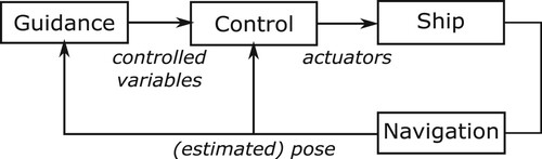
Figure 6 shows the gnc framework. The state is measured directly, which makes the navigation trivial; therefore, it is not discussed further. As already indicated in the introduction, the guidance provides setpoints to the vehicle controller such that the route of the vessel coincides with that of a moving target. The aim of the controller is to alter the actuators such that the vessel state coincides with the required state. The mission state diagram in Figure 3 shows the guidance, controller and allocator for each operational state.

Figure 6. The guidance– navigation– control framework.

4.1. Guidance

4.1.1. Trajectory or constant pose

If the vessel is fully-actuated, then guidance is not really needed, and the output of the trajectory or of a constant pose can be directly provided to the vehicle controller. The smooth transition mechanism, elaborated upon in Section 4.4, will take care that the convergence to this constant pose or trajectory goes smoothly. The poses before and after docking are manually provided at a safe distance from the dock.

4.1.2. Line-of-sight with waypoints

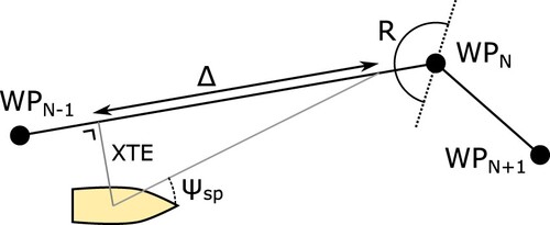
In the transit phase, the route of the vessel is provided by a set of manually entered waypoints. Each waypoint consists of an x, y-position and a required surge speed. The path is defined as straight segment between two consecutive waypoints. The required heading is calculated by means of a los guidance law (Fossen TI 2021), as illustrated in Figure 7. The heading setpoint is calculated as follows: (6) ${\psi }_{\mathrm{sp}}={\arctan }_2(\mathrm{xte},\mathrm{\Delta })+{\psi }_{\mathrm{s}},$(6) in which ${\psi }_{\mathrm{s}}$ is the angle of the segment in a North-East-Down coordinate system. xte and Δ are the cross-track-error and look-ahead distance, respectively. The surge speed setpoint is copied from the previous waypoint. If the vessel comes within an Euclidean distance R of the next waypoint, or passes the line that intersects two successive segments, then the next segment is selected.

Figure 7. The los guidance law calculates the heading setpoint ${\psi }_{\mathrm{sp}}$ based on the cross-track error (xte) and the look-ahead distance Δ. The next segment is started if the ship passes the dotted line, or is within an Euclidean distance R of the next waypoint.

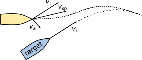
4.1.3. Constant bearing with a trajectory

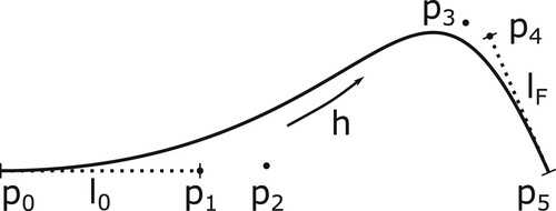
The under-actuated approach phase makes use of a constant bearing guidance law, in combination with a trajectory that brings the vessel from its cruising speed to a safe pose close to the quay. When the bow thrusters become effective, the same trajectory is used, but the cb guidance law is no longer used, as the pose required can be directly provided to the vehicle controller. The cb guidance law is used because it also uses the target speed and hence has enough information to track the target without error.

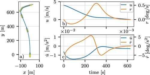
Trajectory an optimal trajectory to a dock can be determined as an ocp (Djouani and Hamam 1995; Ohtsu et al. 1996; Miyauchi et al. 2022). However, solving an ocp can be computationally demanding and might be difficult in real-time applications. In Sawada et al. (2021),de Kruif (2022a), it has been shown that Bézier curves can be used to generate smooth trajectories and their corresponding time derivatives to approach the dock. The computational time to construct the trajectory, including minimisation of the maximum rate-of-turn, mentioned in the Appendix 1, takes less than 0.1 s with Scipy on an Intel i7 1.90 GHz cpu. The acceleration and rate-of-turn values are limited when the trajectory is not too challenging, such as a single turn on an ‘S’-shaped curve. If the ship arrives parallel to the quay and should turn around, then the control points of the Bézier curve are collinear and not in increasing order, see Figure A1. This results in a a ‘cusp’ node with infinite acceleration which cannot be tracked. An ocp approach would be able to handle such a situation. The approach phase is initiated at a distance of about 10 ship lengths. This distance is found to be a good distance to start the approach phase: A larger distance would have the vessel sail straight to this distance, after which the same trajectory results. If a shorter distance would be used, the total duration of the operation would take longer, or it would even become infeasible to dock (de Kruif 2022a). From the current pose a fifth-order Bézier curve is constructed, ending at the manually entered pose close to the dock. We refer to Appendix 1 for the symbols used and the selection of the control points. A Bézier curve is a path in space only, and is dependent on its path variable h. A relation between the path variable and time makes the path a time-dependent trajectory. If we relate the path variable to time as $h=\frac{t{u}_0}{10l_0}(2-\frac{t{u}_0}{10l_0})$, where t denotes time and $u_0$ the initial speed, then we will decrease the speed from $u_0$ to zero. An example trajectory is shown in Figure 8. The trajectory provides us with a target position ${\mathit{p}}_{\mathrm{t}}=[p_{\mathrm{t},x},p_{\mathrm{t},y}{]}^T$ and target velocity ${\mathit{v}}_{\mathrm{t}}=[v_{\mathrm{t},x},v_{\mathrm{t},y}{]}^T$ in Earth-fixed coordinates.

Figure 8. Generated Bézier trajectory. (a) shows the path, while (b) resp. (c) show the velocities and accelerations for surge resp. yaw.

Constant bearing guidance law

A cb guidance law is used to provide a setpoint to the vehicle controller such that the vessel will converge to the target, i.e. the current point of the trajectory, as shown in Figure 9. The setpoint velocity vector, ${\mathit{v}}_{\mathrm{sp}}=[v_{\mathrm{sp},x},v_{\mathrm{sp},y}{]}^T$ to the vehicle controller is given as (Breivik 2010): (7) ${\mathit{v}}_{\mathrm{sp}}={\mathit{v}}_{\mathrm{t}}+{\mathit{v}}_{\mathrm{a}}={\mathit{v}}_{\mathrm{t}}+\gamma \frac{\stackrel{\mathbf{~}}{\mathit{p}}}{||\stackrel{\mathbf{~}}{\mathit{p}}||}\text{with}\stackrel{\mathbf{~}}{\mathit{p}}={\mathit{p}}_{\mathrm{t}}-\mathit{p}.$(7)

Figure 9. The Constant Bearing guidance law. The target has velocity $v_{\mathrm{t}}$. The setpoint to the vessel, $v_{\mathrm{sp}}$ is an addition of the target velocity and an addition $v_{\mathrm{a}}$.

In this equation, the velocity setpoint is composed of the target velocity ${\mathit{v}}_{\mathrm{t}}$ and an added velocity ${\mathit{v}}_{\mathrm{a}}$ which steers the vessel to the current position of the target. The speed and course setpoints to the vehicle controller, $u_{\mathrm{sp}}$ and ${\chi }_{\mathrm{sp}}$, are obtained from: (8) $u_{\mathrm{sp}}=||{\mathit{v}}_{\mathrm{sp}}|{|}_2,{\chi }_{\mathrm{sp}}={\arctan }_2(v_{\mathrm{sp},y},v_{\mathrm{sp},x}).$(8) The value γ results from the distance between the target position and the actual vessel position: (9) $\gamma =U_{\max }\sqrt{{\stackrel{\mathbf{~}}{\mathit{p}}}^T\stackrel{\mathbf{~}}{\mathit{p}}}/\sqrt{({\stackrel{\mathbf{~}}{\mathit{p}}}^T\stackrel{\mathbf{~}}{\mathit{p}}+{\mathrm{\Gamma }}^2)}.$(9) The parameter $U_{\max }$ is the maximum speed at which our vessel is moving towards the target point, and Γ is the distance at which $U_{\max }$ is halved.

4.2. Vehicle control

The vehicle controllers calculate the forces that are needed to control the vessel. These are mapped to the actuators by the allocation algorithm, treated in §4.3.

4.2.1. 3 × PD controller

Independent pd controllers are used for each of the three degrees of freedom. These controllers are used for low speeds when the bow thrusters are active, and where the system behaves as a moving mass as treated in section 3.2.1. The control forces are calculated at the cog. The gains are calculated by pole placement, as shown in Appendix C.1. An integral term has been implemented to counteract low-frequency drift, but was set to zero in the experiments as this drift was not found to be an issue.

4.2.2. Autopilot

The autopilot used is divided into a speed controller and a heading controller. The speed controller is designed as a pi controller by means of pole placement and calculates the longitudinall force. The poles of the heading controller are placed such that it mimics a second order system. The heading controller calculates the lateral force at the location of the stern azimuthing thrusters. We refer to Appendix C.2 for the equations for the gains.

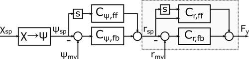
4.2.3. Approaching controller

The controller for the under-actuated approach phase is designed as a cascade controller, as shown in Figure 10. This approach is used so that the non-linearities and the unstable pole of the inner-loop can be addressed first. The resulting inner-loop then becomes stable, which allows for a simple outer-loop design. A single loop compensator with an unstable zero and pole would otherwise lead to a high sensitivity peak (Skogestad and Postlethwaite 2007). The gains and calculations are given in C.3. Note that the time-derivatives ${\dot{r}}_{\mathrm{sp}}$ and ${\dot{\psi }}_{\mathrm{sp}}$ are not calculated by numerical derivation, as implied by Figure 10. These signals can be derived from the known course setpoints, see Appendix C.3. The lateral force $F_y$ is applied at the location of the azimuthing thrusters. Before it is provided to the allocation algorithm it is mapped to the cog.

Figure 10. Control setup for the course control. The controller for the rate-of-turn $C_r$ contains a feedback (fb) and feedforward (ff) part. The inner-loop is depicted in the grey box. The rate-of-turn setpoint is provided by the controller of the outer-loop $C_{\psi }$. The required heading is calculated in the block $\chi \to \psi$. The ‘s’ blocks denote time differentiation. The subscripts ‘mv’ and ‘sp’ are used for measured value and setpoint, respectively.

In the previous work, a course controller was used (de Kruif 2023). However, the fluctuations in course are much larger than the fluctuations in heading due to the waves, therefore, the experiments were conducted with a heading controller. This implies that the direction in which to move, the course χ, has to be converted to a heading ψ. This conversion is done based on the identified relation from a detailed numerical model of the vessel (5(5) $\frac{\chi }{\psi }=\frac{c{s}^2+(1+b)s+a}{s+a}=\frac{({\tau }_{z_1}s+1)({\tau }_{z_2}s+1)}{{\tau }_{p}s+1},$(5) ). In this equation ${\tau }_{z_2}$ is associated with a zero in the right-half plane. If it would be inverted, then the heading setpoint would grow unboundedly. Therefore, only the stable part is inverted, see C.3.

4.3. Allocation

The feeder vessel is equipped with two stern azimuthing thrusters and two bow tunnel thrusters. The thruster properties are presented in Table 3. A quadratic relation between rpm and the thrust is determined, based on captive model tests.

Table 3. Azimuthing and bow thruster parameters.

		azimuth	bow
diameter	D	1.5	1.0	m
maximum power	$P_{max}$	49	0.2	MW
maximum thrust	$T_{max}$	500	200	kN
maximum rpm	${\mathrm{rpm}}_{max}$	644	786	min${}^{-1}$
rudder speed	${\dot{\delta }}_{max}$	18	–	deg/s
forbidden zone ps		$[255,285]$	–	deg
forbidden zone sb		$[75,105]$	–	deg

For the azimuthing thrusters, setpoints for rpm and azimuth angle can be specified. For the bow tunnel thrusters, a setpoint for rpm can be specified. The allocation algorithm distributes the required surge and sway forces and the yaw moment over the available thrusters. Bow tunnel thrusters become less effective with increasing forward speed. The mission execution accounts for this, by activating the bow tunnel thrusters only at speeds below 0.5 m/s. Above this threshold only the stern azimuthing thrusters are used. This requires a switch in the allocation from forces to actuator settings. A similar swich is found in Rethfeldt et al. (2021), albeit with pump-jets. The allocation problem is defined as an optimisation problem, where the minimum of an objective function is sought while respecting constraints. The objective function is defined as the sum of the powers $P_i$ of all active thrusters $T_i$: (10) $J=\sum _i{P}_i=\sum _i{c}_i{T}_i^{3/2}.$(10) where the thrust-to-power coefficient $c_i$ is found from the maximum thrust and power. The active thrusters must provide the required surge and sway forces and yaw moment: (11) $\begin{array}{rl}& \sum _i{T}_i\cos {\delta }_i=F_x,\sum _i{T}_i\sin {\delta }_i=F_y,\\ & \sum _i{T}_i(r_{x,i}\cos {\delta }_i-r_{y,i}\sin {\delta }_i)=M_z.\end{array}$(11) where $(r_{x,i},r_{y,i})$ is the thruster position with respect to the vessel's center of gravity, ${\delta }_i$ its angle, and $F_x,F_y,$ and $M_z$ the force in longitudinal, the force in lateral direction and moment around the vertical axis respectively. Extra inequality constraints express saturation (maximum thrust) and forbidden zones as specified in Table 3.

4.4. Smooth state transitions

When the operational states are combined to shape the whole operation, switching the gnc elements should not introduce excessive transients. Figure 11 depicts our approach to get continuous signals when switching. It is related to the approach in Alessandri et al. (2019) which avoids bumps by setting the new setpoint equal to the last measured value. However, starting with an error of zero does not guarantee a continuous control signal without the use of an offset to the output ${\mathrm{\Delta }}_{\mathrm{u}}$. In Walmsness et al. (2023), the internal (integrator) state is used to guarantee this continuity. The scheme proposed in Figure 11 does not need to know internal signals to achieve continuity.

Figure 11. Scheme used to smoothly transition between controllers. The signals ${\mathrm{\Delta }}_{\mathrm{sp}}$ and ${\mathrm{\Delta }}_{\mathrm{u}}$ vanish in time, make the control signal continuous.

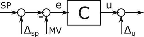
Let Figure 11 illustrate the controller that just became active. It receives an external setpoint (sp) and measured value (mv). The signal ${\mathrm{\Delta }}_{\mathrm{sp}}$ is added to the setpoint that goes to zero in a fixed amount of time $T_{\mathrm{e}}$. This signal is chosen such that the error to the controller starts at zero at switching time $t=\tau$, e.g. ${\mathrm{\Delta }}_{\mathrm{sp}}(t)=(\mathrm{mv}(\tau )-\mathrm{sp}(\tau ))P(t-\tau ,T_{\mathrm{e}})$, where P is the polynomial $P(t,1)=1-10t^3+15t^4-6t^5$ that goes from 1 to 0 and has zero first and second derivatives. Next to a change in the setpoint, the similar signal is added to the output. Again, this signal is selected such that it goes to zero in a fixed time period, $T_{\mathrm{u}}$, and that the initial output of the controller equals the output of the control signal before the switch: ${\mathrm{\Delta }}_{\mathrm{u}}=(u({\tau }^{-})-u({\tau }^{+}))P(t-\tau ,T_{\mathrm{u}})$. Typically, $T_{\mathrm{u}}\ll T_{\mathrm{e}}$. These choices make the control signal continuous, but not necessarily differentiable.

5. Experiments

5.1. Experimental setup

5.1.1. Feeder vessel

The experiments are conducted with scale model shown in Figure 1. All parameters are scaled by means of Froude scaling. There are no mechanical connections between the model and the shore during the experiments. The computations needed for the control are all done on board, and the required energy comes from a battery inside the model. An Earth-fixed pose measurement system, which mimics gps, is available from an optical position measurement system with dedicated targets on the model. Linear velocities are based on these measurements by means of an $\alpha -\beta$ tracker. The rate-of-turn is measured by a rate-gyro.

Six ducted fans are placed on the model to create wind disturbances. The thrust of these fans results from the heading and the wind coefficients from cfd calculations (Daalen et al. 2023). Thrust-rpm curves were measured beforehand.

Initial manoeuvring tests showed that the model is course unstable, as predicted by the cfd calculations. This implies a hysteresis loop that we have to overcome if we want to turn the model to the other direction (Nomoto 1972).

5.1.2. Seakeeping and manoeuvring basin

The experiments were done in Marin's Seakeeping and Manoeuvring Basin. This basin has physical dimensions of 170 m by 40 m, and a water depth of 5 m. These dimensions become 2890 m by 680 m and 85 m deep when converted to full-scale. The basin is fitted with flap-type wave makers on two adjacent sides. The waves are distributed according to a Pierson-Moskowitz spectrum. A quay with fenders was placed in the basin.

5.1.3. Control tuning

The vehicle controllers were tuned by increasing their bandwidth until they hit some limitation. The limitation found was excessive roll, for the pd controllers in sway- and heading-direction, and for the heading control of the autopilot and approaching controller. The pd controller in surge-direction was limited due to the capacity of the azimuthing thrusters. The speed controllers, however, were tuned at a lower bandwidth. This was done to avoid frequent turning of the azimuthing thrusters, which would impede the directional control. The same approach is used to tune the parameters in the guidance law (6(6) ${\psi }_{\mathrm{sp}}={\arctan }_2(\mathrm{xte},\mathrm{\Delta })+{\psi }_{\mathrm{s}},$(6) ) and (9(9) $\gamma =U_{\max }\sqrt{{\stackrel{\mathbf{~}}{\mathit{p}}}^T\stackrel{\mathbf{~}}{\mathit{p}}}/\sqrt{({\stackrel{\mathbf{~}}{\mathit{p}}}^T\stackrel{\mathbf{~}}{\mathit{p}}+{\mathrm{\Gamma }}^2)}.$(9) ): decrease the $\mathrm{\Delta },\mathrm{\Gamma }$ until oscillations occurred. The values used in all the experiments were $\mathrm{\Delta }=2L_{\mathrm{pp}}$ and $\mathrm{\Gamma }=50$ m. The radius R in Figure 7 is always set to 2.5 m.

The transition times $T_{\mathrm{u}}$ was set to 10 s to spin up the thrusters slowly. The transition time $T_{\mathrm{e}}$ was set quite arbitrary to 150 s, except during the point-to-point motions of the (un)docking phase, where it was set to 250 s.

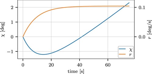
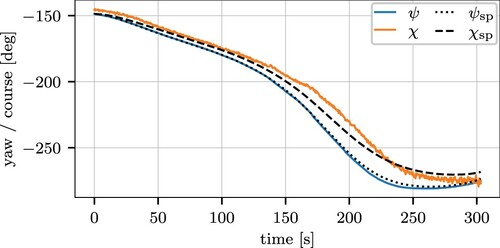
The tracking performance of the underactuated cascade controller is shown in Figure 12. The heading is directly controlled, and its measurement coincides well with its reference signal. The heading setpoint is calculated from the course setpoint. The required course is indicated by the dashed line. The measured course is indicated by the orange line. The course is not tracked as well as the heading, as it is not controlled directly. Mismatches in the relation between numerical and scale-model will introduce errors. This behaviour is echoed in the experiments.

Figure 12. Results of tuning the cascade controller used for the approach phase.

5.2. Experiments

5.2.1. Round trip

The results of the round-trip without disturbances are shown in Figure 13. In all experiments the vessel could sail the round-trip and safely dock at the quay. In Figure 13(a) the black dots on the track indicate when the operational state was switched, and they coincide with the dashed lines in Figure 13(b) till d). The dot at $(x,y)\approx (600,-50)$, and $t\approx 1225$s is the start of the approach to the quay. The dotted line indicates the Bézier curve the vessel has to sail.

Figure 13. The full round-trip in the smb with the operational phases. In subfigure (d) the azimuth angle is denoted by ${\delta }_{\mathrm{azi}}$ and the telegraph setting for azimuting- and bow thrusters is denoted by $t_{\mathrm{azi}},t_{\mathrm{bt}}$, respectively. sog denotes the speed over ground. The dotted lines show the setpoints. All results are presented in full-scale.

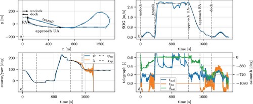
The gnc framework worked as expected throughout the different operational states. At the start and end of the experiment, during the undock/dock phase, the vessel moved smoothly from its current pose to target pose. The smooth transitions took care that there was no jump in the settings.

After the undocking, the vessel sailed around the smb in the transit phase. The heading setpoint, received from the los law, is tracked correctly as shown in Figure 13(c) between $t\approx 200$ sec and $t\approx 1225$ sec. But, inherently, there is some phase lag. Changes in the heading give rise to significant drift angles; this is visible in the turn around x = 1200 m. The speed shown in Figure 13(b) shows that the speed deviates from its setpoint at large heading changes. When the ship is sailing straight, the speed is better retained, e. g. $t\approx 500$ s till $t\approx 800$ s.

The approach phase brought the vessel to the safe pose with zero speed. The cb provided speed and course setpoints that the vehicle controller could track, after the course was converted to a heading. The conversion is not perfect, and a difference between the setpoint and measured course can be seen in Figure 13(c), similar to the result found during the tuning in Figure 12. The cb law will update its course setpoint if the vessel position deviates from the requested trajectory.

Two reasons can explain the difference in calculated and measured course. First, there is a likely mismatch between the parameters a, b and c, see §3.2.4, between the model and the real system. Second, the inversion of transfer function (5(5) $\frac{\chi }{\psi }=\frac{c{s}^2+(1+b)s+a}{s+a}=\frac{({\tau }_{z_1}s+1)({\tau }_{z_2}s+1)}{{\tau }_{p}s+1},$(5) ) omitted the zero in the right-half plane to get a stable inverse and this will introduce an error. However, as the bow thrusters become effective at u<0.5 m/s, the heading and the position are independently controlled and the remainder of the trajectory is tracked such that the vessel ends at zero speed at the safe pose.

Figure 13(d) shows the actuator usage during the manoeuvre. The bow thrusters are only used at low velocities, and not during the transit and the under-actuated approach phase. The large noisy bow thruster commands at near standstill stand out. Because the thrust relates quadratically to the telegraph, small changes due to the noise at low thrust give rise to significant changes in the telegraph setting. The rudder speed, indicated in Table 3 did not pose a limiting factor. When it was decreased below 10 deg/s, its effects became clear in the performance of this experiment.

5.2.2. Disturbances

The previous trajectory is again used, but we now introduce wind and waves disturbances for low-, medium- and high-disturbance levels. Three directions of the wind and the waves are tested. The angle is the direction to where the wind is blowing, i.e. ${\psi }_{\mathrm{ww}}={90}^{\circ }$ indicates that it blows along the Earth-fixed y-axis. Only the paths from the approaching phase onwards are shown in Figure 14. The trip around the basin provided no surprising results. Each path in the figure has its own reference depending on where the approaching phases started. Obviously, they all end at the same pose. Some statistics are gathered in Table 4.

Figure 14. The resulting paths for wind and waves of different magnitude and direction.

The resulting paths for different wind and waves disturbances.

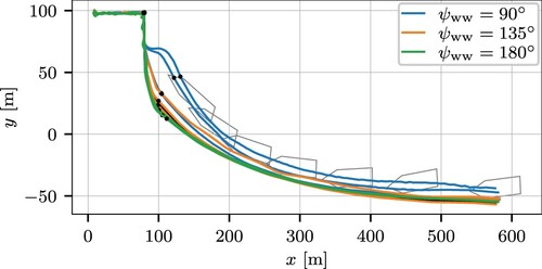
Table 4. Results for distance d to the trajectory, speed error $\tilde{u}$ and heading error $\tilde{\psi }$ for different disturbance levels and directions.

		Approach ua			Approach fa					dock
${\psi }_{\mathrm{ww}}$	dist.	$\overline{d}$	$d_{\mathrm{end}}$	${\tilde{u}}_{\mathrm{rms}}$	$\overline{d}$	$d_{\mathrm{end}}$	${\tilde{u}}_{\mathrm{rms}}$	${\tilde{\psi }}_{\mathrm{rms}}$	${\tilde{\psi }}_{\mathrm{end}}$	$\overline{d}$	$d_{\mathrm{end}}$	${\tilde{u}}_{\mathrm{rms}}$	${\tilde{\psi }}_{\mathrm{rms}}$	${\tilde{\psi }}_{\mathrm{end}}$
(deg)	level	(m)	(m)	(m/s)	(m)	(m)	(m/s)	(deg)	(deg)	(m)	(m)	(m/s)	(deg)	(deg)
–	–	8.04	9.90	0.05	0.35	0.25	0.01	0.99	0.19	1.07	0.14	0.02	0.62	−0.27
90	low	4.69	1.08	0.06	0.40	0.30	0.03	0.85	0.45	0.80	0.07	0.03	0.56	−0.13
90	mid	13.19	23.86	0.10	0.64	0.44	0.04	1.20	0.36	0.90	0.12	0.04	0.68	−0.24
90	high	20.44	31.27	0.14	1.19	0.83	0.09	2.54	0.63	1.09	0.16	0.06	0.92	−0.33
135	low	7.86	11.69	0.05	0.41	0.40	0.02	0.97	0.77	0.78	0.17	0.04	0.65	−0.42
135	mid	3.07	6.23	0.06	0.72	0.60	0.04	1.50	0.77	0.77	0.52	0.07	0.79	−1.06
135	high	5.81	1.18	0.11	1.08	1.48	0.09	1.71	2.49	1.14	1.03	0.17	1.45	−2.39
180	low	6.61	12.88	0.05	0.77	0.56	0.06	1.58	1.00	0.87	0.50	0.09	1.20	−0.60
180	mid	10.56	13.08	0.05	1.21	1.02	0.10	1.47	−0.77	1.08	0.44	0.22	1.46	0.02
180	high	6.52	12.50	0.09	2.10	1.28	0.19	2.19	1.55	1.32	1.13	0.32	1.93	2.24

Note: The rms and end value are presented , indicated by the subscript ‘end’ and ‘rms’. $\overline{d}$ is the mean distance.. The three disturbance levels have wind speed, significant wave height and wave period of $(u_{\mathrm{wind}},H_{\mathrm{s}},T_{\mathrm{p}})$ = (4.60 m/s, 0.5 m, 4.25 s), (6.72 m/s, 0.83 m, 4.58 s), and (8.85 m/s, 1.23 m, 5.22 s) respectively.

The two paths that stand out in Figure 14 correspond to the highest two disturbance levels with ${\psi }_{\mathrm{ww}}={90}^{\circ }$. With these disturbances, even if the vessel sailed a straight course before it started with the approach, a drift angle was needed to counter the effect of the wind and waves. This constant drift is not incorporated in the relation between the course and the heading, and hence the heading setpoint contains errors. Again, the vessel sails to the correct pose when the bow thrusters become active.

Furthermore, as one can see in Table 4, the velocity and heading errors ${\tilde{u}}_{\mathrm{rms}}$ and ${\tilde{\psi }}_{\mathrm{rms}}$ correlate well with the disturbance level. Inspection of these signals show that the vessel, obviously, moves with the waves. These motions dominate the rms error in speed and cannot, and should not, be compensated for with the actuators at hand. Finally, as one would expect, the speed errors are most pronounced when the disturbances come from the beam. Still, the vessel could dock with all the tested disturbances.

Although not shown, the actuators reacted to first-order wave effects. This effect could have been reduced by means of a wave filter (Hassani et al. 2013). Because the feeder vessel sails at different speeds and headings, the encounter spectrum would change, and an adaptive wave frequency would be necessary. In order to keep the experiment as simple as possible, and minimise the amount of parameters to tune, this has not been included.

5.2.3. Approach by waypoints

A comparison has been made for the approach to the dock between an autopilot with a los guidance law used in the preceding transit phase, and the introduced cascade controller with a cb guidance law. If the first method would result in adequate performance, then the separate controller and guidance law for the approach phase are not needed to berth the vessel, which would simplify the design. Figure 15 shows the results if the approach phase is omitted and waypoints are placed on the Bézier trajectory. The blue line indicates the path during the approach phase with the cb law and the cascade controller. The dotted line depicts the Bézier curve. The orange line is for the path for the los law with the autopilot. It has been mirrored in the y = 97.8 m axis for a better presentation. The dots show the waypoints used. The trajectory provided was challenging in surge acceleration and by a large rate-of-turn.

Figure 15. The approach to the dock with the cb and cascade control in comparison with tracking waypoint.

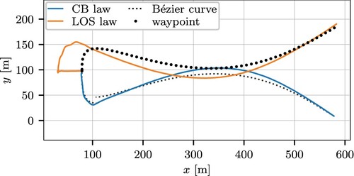
The under-actuated cascade controller tracked the curve not as good as previously in Figure 13. The maximum error was slightly under 17 m. Note that this is the maximum distance to the time-dependent trajectory. The distance to the path was slightly over 10 m. The larger changes in velocity contributed to the larger trajectory error. As before, when the bow thrusters become active, the vessel is brought to the original trajectory, and the distance at the end of the approach was less than 1 m.

The autopilot in combination with the los algorithm gave a much larger error. It was slightly under 100 m. This is as expected, as this guidance and control combination are mainly used for sailing a straight track. In our implementation, there was no feedforward on the required rate-of-turn, nor was there anything implemented to sail smooth curves. If these would be implemented, the error would be much smaller, and the implementation would get closer to the proposed cascade controller.

5.2.4. Transition between phases / dock phase

The final result shown in Figure 16 shows the behaviour when switching from the approach phase to the dock phase and the whole of the dock phase. Only the heading and the behaviour of the azimuthing thruster are shown. The switch occurs at $t\approx 125$ s. A heading setpoint is constructed that coincides with the current measurement and goes to the (constant) setpoint. Without the ${\mathrm{\Delta }}_{\mathrm{u}}$ introduced in Figure 11 this would result in an initial zero telegraph setting. However, a transition from the previous setting in $T_{\mathrm{u}}=10$ s was used to avoid this discontinuity.

Figure 16. Switching from the approach to the docking phase.

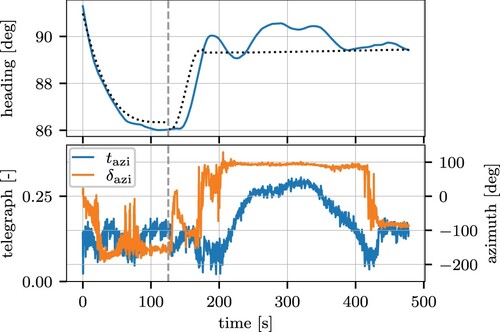
The three pd controllers that moved the vessel from the safe pose to the dock basically act as a dynamic positioning system. The rms heading error in the docking phase is ${\tilde{\psi }}_{\mathrm{rms}}=0.62$ deg during a lateral motion of 71 m. The largest error occurs when the thruster provides the highest thrust. This implies that the thrust is not applied perfectly at the cog. The undocking phase gives similar results and is therefore not shown.

6. Conclusions

A set of experiments was performed at Marin's smb in which an 1:17 scale model of a feeder vessel sailed from one quay to the next. The quay-to-quay mission was first divided into several operational phases, each of these phases was solved in a Guidance-Navigation-Control framework, and finally they were combined while paying attention to smooth switching between the phases. The approach was tested with different wave and wind disturbance levels, and with different routes. In all tests, the mission was completed successfully and the ship docked safely at the quay.

The approach to the quay was found most challenging: the course as well as the speed changed significantly, the manoeuvrability decreased with lower speeds, and the system changed from under-actuated to fully-actuated half-way the trajectory. However, the under-actuated half performed well through a combination of a trajectory based on a Bézier curve with a Constant Bearing guidance law, and a cascade controller as vehicle controller. The errors that did occur were nullified in the fully-actuated part such that the vessel arrived at the safe pose with near-zero velocity. The guidance also provided time derivatives of the controlled variables which could be used in a feedforward controller to improve the performance. When the approach was done by a los guidance law and an autopilot, then the results were not as good.

In this work, a switching mechanism was introduced that took care that there were no discontinuities between the phases. However, the derivatives were not smooth. Although higher order continuity was tested, it was based on unfiltered signals which generated highly fluctuating setpoints. It is recommended for the future work that continuity of the setpoints' derivatives makes use of filtered signals.

An important component in the approach to the dock was the conversion from course to heading. In the future work, this ought to be given more attention. A better heading setpoint is expected by (i) identifying the parameters instead of using the model values, (ii) use the zpetc approach to calculate the inverse (Tomizuka 1987), and (iii) incorporate the influence of the environment on the drift angle.

The aim of this work was on sailing from one quay to the next. In real operations there will be other ships in the vicinity. Collision avoidance with respect to local regulations need to be incorporated into this approach.

Disclosure statement

No potential conflict of interest was reported by the author(s).

Additional information

Funding

MOSES project has received funding from the European Union's Horizon 2020 research & innovation programme under grant agreement No. 861678. Content reflects only the authors' view and the Agency is not responsible for any use that may be made of the information it contains.

Appendices

Appendix 1. Bézier curve

The target position is based on a fifth-order Bezier curve (Kamermans 2022): (A1) $\begin{array}{rl}{\mathit{p}}_{\mathrm{t}}(h)& =(1-h{)}^5{\mathit{p}}_0+5(1-h{)}^{4}h{\mathit{p}}_1+10(1-h{)}^3{h}^2{\mathit{p}}_2\\ & +10(1-h{)}^2{h}^3{\mathit{p}}_3+5(1-h)h^4{\mathit{p}}_4+h^5{\mathit{p}}_5,\end{array}$(A1) where h is the path variable with $0\le h\le 1$. The subscript ‘t’ stands for ‘target’. The variables used are shown in Figure A1 with ${\mathit{p}}_{\mathrm{t}}=[p_{\mathrm{t},x},p_{\mathrm{t},y}{]}^T$ and ${\mathit{p}}_i=[p_{i,x},p_{i,y}{]}^T$. For h = 0, the above expression evaluates to ${\mathit{p}}_{\mathrm{t}}(0)={\mathit{p}}_0$, and for h = 1 we get ${\mathit{p}}_{\mathrm{t}}(1)={\mathit{p}}_5$. The initial and final positions can be used to set ${\mathit{p}}_0,{\mathit{p}}_5$. The derivative with respect to h is calculated as follows: (A2) $\begin{array}{rl}\frac{\mathrm{d}{\mathit{p}}_{\mathrm{t}}}{\mathrm{d}h}(h)& =5(1-h{)}^4({\mathit{p}}_1-{\mathit{p}}_0)+\\ & 20(1-h{)}^{3}h({\mathit{p}}_2-{\mathit{p}}_1)+30(1-h{)}^2{h}^2({\mathit{p}}_3-{\mathit{p}}_2)\\ & +20(1-h)h^3({\mathit{p}}_4-{\mathit{p}}_3)+5h^4({\mathit{p}}_5-{\mathit{p}}_4).\end{array}$(A2) At h = 0 and h = 1, this evaluates to $\frac{\mathrm{d}{\mathit{p}}_{\mathrm{t}}}{\mathrm{d}h}(0)=5({\mathit{p}}_1-{\mathit{p}}_0)$ and $\frac{\mathrm{d}{\mathit{p}}_{\mathrm{t}}}{\mathrm{d}h}(1)=5({\mathit{p}}_3-{\mathit{p}}_2)$. So, the tangent at the start and the end are given by the vector to the adjacent control point. This can be used to set the initial and final headings.

Figure A1. The principle variables of a cubic Bezier curve. $p_i$ are the control points, and $0\le h\le 1$ is the path variable.

The second derivative of ${\mathit{p}}_{\mathrm{t}}$ with respect to h evaluates to $\frac{{\mathrm{d}}^2{\mathit{p}}_{\mathrm{t}}}{{\mathrm{d}h}^2}(0)=20({\mathit{p}}_0-2{\mathit{p}}_1+{\mathit{p}}_2)$ and $\frac{{\mathrm{d}}^2{\mathit{p}}_{\mathrm{t}}}{{\mathrm{d}h}^2}(1)=20({\mathit{p}}_5-2{\mathit{p}}_4+{\mathit{p}}_3)$. By setting these to zero, the rate-of-turn will be zero at the start and end of the path.

In order to convert the path into a time-dependent trajectory, the path variable h must be made time-dependent. The target speed can then be calculated as follows: (A3) $\begin{array}{rl}{u}_{\mathrm{t}}(t)& =\sqrt{{\left(\frac{\mathrm{d}{p}_{\mathrm{t},x}}{\mathrm{d}t}\right)}^2+{\left(\frac{\mathrm{d}{p}_{\mathrm{t},y}}{\mathrm{d}t}\right)}^2}\\ & =\frac{\mathrm{d}h}{\mathrm{d}t}\sqrt{{\left(\frac{\mathrm{d}{p}_{\mathrm{t},x}}{\mathrm{d}h}\right)}^2+{\left(\frac{\mathrm{d}{p}_{\mathrm{t},y}}{\mathrm{d}h}\right)}^2}.\end{array}$(A3) Note that the speed is defined to be positive. Evaluating the target speed at h = 0 and h = 1 gives (A4) $u_0=5l_0\frac{\mathrm{d}h(0)}{\mathrm{d}t},u_{\mathrm{f}}=5l_{\mathrm{f}}\frac{\mathrm{d}h(1)}{\mathrm{d}t},$(A4) where $l_0=\Vert {\mathit{p}}_1-{\mathit{p}}_0\Vert$ and $l_{\mathrm{f}}=\Vert {\mathit{p}}_5-{\mathit{p}}_4\Vert$. Since we want to end at zero speed, $u_{\mathrm{f}}=0$ and we want to have $l_{\mathrm{f}}$ finite, we need $\frac{\mathrm{d}h(1)}{\mathrm{d}t}=0$. The polynomial $h(t)=t/T(2-t/T)$, among many others, achieves this. T is the duration of traversing the path. The derivative at t = 0 evaluates to $\frac{\mathrm{d}h(0)}{\mathrm{d}t}=2/T$. This can be related to the initial velocity: (A5) $u_0=\frac{10l_0}{T}\Rightarrow h=\frac{t{u}_0}{10l_0}(2-\frac{t{u}_0}{10l_0}).$(A5) $l_0,l_{\mathrm{f}}$ are the remaining variables that tune the initial and final straight part of the curve. We optimised these with a SciPy minimisation script to get a minimal rate-of-turn and to minimise the maximum speed if it is larger than the initial speed.

Appendix 2. Setpoint derivatives

The setpoint to the vehicle controller is a combination of the Bézier curve and the cb algorithm. The time derivatives of the Bézier curve are found by using the chain rule: (A6) $\begin{array}{rl}{\mathit{v}}_{\mathrm{t}}& =\frac{\mathrm{d}{\mathit{p}}_{\mathrm{t}}}{\mathrm{d}t}=\frac{\mathrm{d}\mathit{p}}{\mathrm{d}h}\frac{\mathrm{d}h}{\mathrm{d}t},\end{array}$(A6) (A7) $\begin{array}{rl}\frac{\mathrm{d}{\mathit{v}}_{\mathrm{t}}}{\mathrm{d}t}& =\frac{{\mathrm{d}}^2{\mathit{p}}_{\mathrm{t}}}{{\mathrm{d}t}^2}=\frac{{\mathrm{d}}^2\mathit{p}}{{\mathrm{d}h}^2}{\left(\frac{\mathrm{d}h}{\mathrm{d}t}\right)}^2+\frac{\mathrm{d}\mathit{p}}{\mathrm{d}h}\frac{{\mathrm{d}}^{2}h}{{\mathrm{d}t}^2}.\end{array}$(A7) These derivatives contain the earth-fixed x- and y-coordinates. The derivative of the setpoint speed to the vehicle controller, (8(8) $u_{\mathrm{sp}}=||{\mathit{v}}_{\mathrm{sp}}|{|}_2,{\chi }_{\mathrm{sp}}={\arctan }_2(v_{\mathrm{sp},y},v_{\mathrm{sp},x}).$(8) ), is (A8) $\frac{\mathrm{d}{u}_{\mathrm{sp}}}{\mathrm{d}t}=\frac{v_{\mathrm{sp},x}\frac{\mathrm{d}}{\mathrm{d}t}{v}_{\mathrm{sp},x}+v_{\mathrm{sp},y}\frac{\mathrm{d}}{\mathrm{d}t}{v}_{\mathrm{sp},y}}{u_{\mathrm{sp}}}.$(A8) ${\mathit{v}}_{\mathrm{sp}}=[v_{\mathrm{sp},x},v_{\mathrm{sp},y}{]}^T$ is known from (7(7) ${\mathit{v}}_{\mathrm{sp}}={\mathit{v}}_{\mathrm{t}}+{\mathit{v}}_{\mathrm{a}}={\mathit{v}}_{\mathrm{t}}+\gamma \frac{\stackrel{\mathbf{~}}{\mathit{p}}}{||\stackrel{\mathbf{~}}{\mathit{p}}||}\text{with}\stackrel{\mathbf{~}}{\mathit{p}}={\mathit{p}}_{\mathrm{t}}-\mathit{p}.$(7) ). The components of the acceleration are a summation of the target acceleration and acceleration to bring the vessel to the target (A9) $\frac{\mathrm{d}{\mathit{v}}_{\mathrm{sp}}}{\mathrm{d}t}=\frac{\mathrm{d}{\mathit{v}}_{\mathrm{t}}}{\mathrm{d}t}+\frac{\mathrm{d}{\mathit{v}}_{\mathrm{a}}}{\mathrm{d}t}.$(A9) The first term on the right-hand side follows from (A7(A7) $\begin{array}{rl}\frac{\mathrm{d}{\mathit{v}}_{\mathrm{t}}}{\mathrm{d}t}& =\frac{{\mathrm{d}}^2{\mathit{p}}_{\mathrm{t}}}{{\mathrm{d}t}^2}=\frac{{\mathrm{d}}^2\mathit{p}}{{\mathrm{d}h}^2}{\left(\frac{\mathrm{d}h}{\mathrm{d}t}\right)}^2+\frac{\mathrm{d}\mathit{p}}{\mathrm{d}h}\frac{{\mathrm{d}}^{2}h}{{\mathrm{d}t}^2}.\end{array}$(A7) ). The second term is calculated as follows: (A10) $\begin{array}{rl}\frac{\mathrm{d}{\mathit{v}}_a}{\mathrm{d}t}& =\frac{\mathrm{d}\gamma }{\mathrm{d}t}\frac{\stackrel{\mathbf{~}}{\mathit{p}}}{||\stackrel{\mathbf{~}}{\mathit{p}}||}+\gamma \frac{\mathrm{d}}{\mathrm{d}t}\left(\frac{\tilde{\mathit{p}}}{||\tilde{\mathit{p}}||}\right),\end{array}$(A10) (A11) $\begin{array}{rl}\frac{\mathrm{d}\gamma }{\mathrm{d}t}& =U_{\max }\frac{{\mathrm{\Delta }}^2({\tilde{p}}_x{\tilde{v}}_x+{\tilde{p}}_y{\tilde{v}}_y)}{{({\tilde{\mathit{p}}}^T\tilde{\mathit{p}}+{\mathrm{\Delta }}^2)}^{\frac{3}{2}}\sqrt{{\stackrel{\mathbf{~}}{\mathit{p}}}^T\stackrel{\mathbf{~}}{\mathit{p}}}},\end{array}$(A11) (A12) $\begin{array}{rl}\frac{\mathrm{d}}{\mathrm{d}t}{\left(\frac{\stackrel{\mathbf{~}}{\mathit{p}}}{||\stackrel{\mathbf{~}}{\mathit{p}}||}\right)}_x& =\frac{(-{\tilde{p}}_x{\tilde{v}}_x-{\tilde{p}}_y{\tilde{v}}_y){\tilde{p}}_x}{{\left({\stackrel{\mathbf{~}}{\mathit{p}}}^T\stackrel{\mathbf{~}}{\mathit{p}}\right)}^{\frac{3}{2}}}+\frac{{\tilde{v}}_x}{\sqrt{{\stackrel{\mathbf{~}}{\mathit{p}}}^T\stackrel{\mathbf{~}}{\mathit{p}}}},\end{array}$(A12) (A13) $\begin{array}{rl}\frac{\mathrm{d}}{\mathrm{d}t}{\left(\frac{\stackrel{\mathbf{~}}{\mathit{p}}}{||\stackrel{\mathbf{~}}{\mathit{p}}||}\right)}_y& =\frac{(-{\tilde{p}}_x{\tilde{v}}_x-{\tilde{p}}_y{\tilde{v}}_y){\tilde{p}}_y}{{\left({\stackrel{\mathbf{~}}{\mathit{p}}}^T\stackrel{\mathbf{~}}{\mathit{p}}\right)}^{\frac{3}{2}}}+\frac{{\tilde{v}}_y}{\sqrt{{\stackrel{\mathbf{~}}{\mathit{p}}}^T\stackrel{\mathbf{~}}{\mathit{p}}}},\end{array}$(A13) in which ${\tilde{v}}_x$ is the difference in the velocity between the target and the ship in the earth fixed x-coordinate. The same holds for the y-component. The time derivative of the course setpoint (8(8) $u_{\mathrm{sp}}=||{\mathit{v}}_{\mathrm{sp}}|{|}_2,{\chi }_{\mathrm{sp}}={\arctan }_2(v_{\mathrm{sp},y},v_{\mathrm{sp},x}).$(8) ) is calculated as follows: (A14) $\frac{\mathrm{d}{\chi }_{\mathrm{sp}}}{\mathrm{d}t}=\frac{v_{\mathrm{sp},x}\frac{\mathrm{d}}{\mathrm{d}t}{v}_{\mathrm{sp},y}-v_{\mathrm{sp},y}\frac{\mathrm{d}}{\mathrm{d}t}{v}_{\mathrm{sp},x}}{u_{\mathrm{sp}}^2}.$(A14) Again, the velocity setpoint follows from (7(7) ${\mathit{v}}_{\mathrm{sp}}={\mathit{v}}_{\mathrm{t}}+{\mathit{v}}_{\mathrm{a}}={\mathit{v}}_{\mathrm{t}}+\gamma \frac{\stackrel{\mathbf{~}}{\mathit{p}}}{||\stackrel{\mathbf{~}}{\mathit{p}}||}\text{with}\stackrel{\mathbf{~}}{\mathit{p}}={\mathit{p}}_{\mathrm{t}}-\mathit{p}.$(7) ). It's derivative is the sum of $\frac{\mathrm{d}{\mathit{v}}_{\mathrm{t}}}{\mathrm{d}t}$ (A7(A7) $\begin{array}{rl}\frac{\mathrm{d}{\mathit{v}}_{\mathrm{t}}}{\mathrm{d}t}& =\frac{{\mathrm{d}}^2{\mathit{p}}_{\mathrm{t}}}{{\mathrm{d}t}^2}=\frac{{\mathrm{d}}^2\mathit{p}}{{\mathrm{d}h}^2}{\left(\frac{\mathrm{d}h}{\mathrm{d}t}\right)}^2+\frac{\mathrm{d}\mathit{p}}{\mathrm{d}h}\frac{{\mathrm{d}}^{2}h}{{\mathrm{d}t}^2}.\end{array}$(A7) ) and $\frac{\mathrm{d}{\mathit{v}}_{\mathrm{a}}}{\mathrm{d}t}$ (A10(A10) $\begin{array}{rl}\frac{\mathrm{d}{\mathit{v}}_a}{\mathrm{d}t}& =\frac{\mathrm{d}\gamma }{\mathrm{d}t}\frac{\stackrel{\mathbf{~}}{\mathit{p}}}{||\stackrel{\mathbf{~}}{\mathit{p}}||}+\gamma \frac{\mathrm{d}}{\mathrm{d}t}\left(\frac{\tilde{\mathit{p}}}{||\tilde{\mathit{p}}||}\right),\end{array}$(A10) )–(A13(A13) $\begin{array}{rl}\frac{\mathrm{d}}{\mathrm{d}t}{\left(\frac{\stackrel{\mathbf{~}}{\mathit{p}}}{||\stackrel{\mathbf{~}}{\mathit{p}}||}\right)}_y& =\frac{(-{\tilde{p}}_x{\tilde{v}}_x-{\tilde{p}}_y{\tilde{v}}_y){\tilde{p}}_y}{{\left({\stackrel{\mathbf{~}}{\mathit{p}}}^T\stackrel{\mathbf{~}}{\mathit{p}}\right)}^{\frac{3}{2}}}+\frac{{\tilde{v}}_y}{\sqrt{{\stackrel{\mathbf{~}}{\mathit{p}}}^T\stackrel{\mathbf{~}}{\mathit{p}}}},\end{array}$(A13) ). The result of $\frac{{\mathrm{d}}^2{\chi }_{\mathrm{sp}}}{{\mathrm{d}t}^2}$ is not shown here, but is available as supplementary material.

Appendix 3. Controllers

A.1. 3×PD controller

Each dof is controlled independently. With transfer function $P(s)=1/m{s}^2$, and controller $C(s)=K_{\mathrm{p}}+s{K}_{\mathrm{d}}$, we get the characteristic equation: (A15) $\xi (s)=s^2+s{K}_{\mathrm{d}}/m+K_{\mathrm{p}}/m.$(A15) If we place its roots to obtain a damped second-order system, then we find the gains (A16) $\begin{array}{rl}& s^2+s{K}_{\mathrm{d}}/m+K_{\mathrm{p}}/m=s^2+2\zeta {\omega }_{\mathrm{n}}s+{\omega }_{\mathrm{n}}^2\Rightarrow \\ & K_{\mathrm{p}}=m{\omega }_{\mathrm{n}}^2,K_{\mathrm{d}}=2\mathrm{m\zeta }{\omega }_{\mathrm{n}},\end{array}$(A16) where ${\omega }_{\mathrm{n}}$ is the natural frequency and ζ is the relative damping.

A.2. Autopilot

The autopilot is divided into a heading controller and a speed controller. Similar to the previous section, we calculate the characteristic equation based on (3(3) $\frac{r}{F_y}=\frac{K/T}{s+\mathrm{\alpha K}/T}\to \frac{\psi }{F_y}=\frac{K/T}{s(s+\mathrm{\alpha K}/T)}.$(3) ): (A17) $\frac{\psi }{F_y}=\frac{K/T}{s(s+\mathrm{\alpha K}/T)}.$(A17) Placing the roots of the characteristic equation to mimic a second order system, we obtain (A18) $K_{\mathrm{p}}={\omega }_{\mathrm{n}}^2(T/K),K_{\mathrm{d}}=2\zeta {\omega }_{\mathrm{n}}(T/K)-\alpha .$(A18) The values of the parameters can be found in Table 2. The speed model (1(1) $m_x\dot{u}=m_x\mathrm{vr}+X_{u|u|}u|u|+F_x,$(1) ) linearised around zero speed provides the transfer function: $P(s)=1/\mathrm{ms}$. When this is controlled by a pi controller $C_{u,\mathrm{fb}}(s):F_x/\tilde{u}=(s{K}_{\mathrm{p}}+K_{\mathrm{i}})/s$, we find with pole-placement the gains (A19) $K_{\mathrm{i}}={\omega }_{\mathrm{n}}^{2}m,K_{\mathrm{p}}=2\zeta {\omega }_{\mathrm{n}}m.$(A19) A feedforward controller is used to improve changes in the setpoint (A20) $C_{u,\mathrm{ff}}:F_x=(m-X_{\dot{u}}){\dot{u}}_{\mathrm{sp}}+X_{u|u|}{u}_{\mathrm{sp}}|u_{\mathrm{sp}}|.$(A20)

A.3. Approaching controller

Inner-loop: The feedforward signal can be calculated directly from (2(2) $\dot{r}=-\frac{K}{T}(\alpha +\beta r^2)r+\frac{K}{T}{F}_y.$(2) ) (A21) $C_{r,\mathrm{ff}}:F_y=\alpha r_{\mathrm{sp}}+\beta r_{\mathrm{sp}}^3+\frac{T}{K}{\dot{r}}_{\mathrm{sp}}.$(A21) The feedback controller is based on (3(3) $\frac{r}{F_y}=\frac{K/T}{s+\mathrm{\alpha K}/T}\to \frac{\psi }{F_y}=\frac{K/T}{s(s+\mathrm{\alpha K}/T)}.$(3) ). When the loop is closed with (A22) $C_{r,\mathrm{fb}}:F_y=K_{\mathrm{r}}(r_{\mathrm{sp}}-r),$(A22) we obtain the closed-loop transfer function (A23) $\frac{r}{r_{\mathrm{sp}}}=\frac{K_{\mathrm{r}}K/T}{s+K/T(\alpha +K_{\mathrm{r}})}.$(A23) A feedback gain $K_{\mathrm{r}}>-\alpha$ will stabilise this system (Neuffer and Owens 1992).

Outer-loop: The outer-loop provides a rate-of-turn setpoint. The transfer from this setpoint to the heading follows from (A23(A23) $\frac{r}{r_{\mathrm{sp}}}=\frac{K_{\mathrm{r}}K/T}{s+K/T(\alpha +K_{\mathrm{r}})}.$(A23) ): (A24) $\frac{\psi }{r_{\mathrm{sp}}}=\frac{K_{\mathrm{r}}K/T}{s(s+K/T(\alpha +K_{\mathrm{r}}))}.$(A24) Closing this system with (A25) $C_{\psi ,\mathrm{fb}}:r_{\mathrm{sp}}=K_{\psi }({\psi }_{\mathrm{sp}}-{\psi }_{\mathrm{mv}})$(A25) results in the characteristic equation, which we can equate to the poles of a second-order system: (A26) $\xi (s)=s^2+s(K/T)(\alpha +K_{\mathrm{r}})+K_{\psi }{K}_{\mathrm{r}}(K/T)=s^2+2\zeta {\omega }_{\mathrm{n}}s+{\omega }_{\mathrm{n}}^2$(A26) from which the gains directly follow. The feedforward path is trivially written as follows: (A27) $C_{\psi ,\mathrm{ff}}:r_{\mathrm{sp}}={\dot{\psi }}_{\mathrm{sp}}.$(A27) Note that $r_{\mathrm{sp}}$ in Figure 10 is not calculated by numerical differentiation, but by taking the derivatives of (A25(A25) $C_{\psi ,\mathrm{fb}}:r_{\mathrm{sp}}=K_{\psi }({\psi }_{\mathrm{sp}}-{\psi }_{\mathrm{mv}})$(A25) ) and (A27(A27) $C_{\psi ,\mathrm{ff}}:r_{\mathrm{sp}}={\dot{\psi }}_{\mathrm{sp}}.$(A27) ).

From course to heading:

The transfer from heading to course is repeated from (5(5) $\frac{\chi }{\psi }=\frac{c{s}^2+(1+b)s+a}{s+a}=\frac{({\tau }_{z_1}s+1)({\tau }_{z_2}s+1)}{{\tau }_{p}s+1},$(5) ): (A28) $\frac{\chi }{\psi }=\frac{({\tau }_{z_1}s+1)({\tau }_{z_2}s+1)}{{\tau }_{p}s+1}$(A28)

in which ${\tau }_{z_2}$ places the zero in the right-half plane. The heading setpoint is calculated as the stable part of the inverse (A29) $\frac{{\psi }_{\mathrm{sp}}}{{\chi }_{\mathrm{sp}}}=\frac{{\tau }_{p}s+1}{{\tau }_{z_1}s+1}.$(A29) This can be written in state space as follows: (A30) $\begin{array}{rl}\dot{x}& =\mathrm{Ax}+B{\chi }_{\mathrm{sp}},\end{array}$(A30) (A31) $\begin{array}{rl}{\psi }_{\mathrm{sp}}& =\mathrm{Cx}+D{\chi }_{\mathrm{sp}},\end{array}$(A31) with $A=-1/{\tau }_{z_1},B=({\tau }_{z_1}-{\tau }_p)/{\tau }_{z_1}^2,C=1,$ and $D={\tau }_p/{\tau }_{z_1}$. From this the derivatives can be calculated as follows: (A32) $\begin{array}{rl}{\dot{\psi }}_{\mathrm{sp}}& =C\dot{x}+D{\dot{\chi }}_{\mathrm{sp}}=C(\mathrm{Ax}+B{\chi }_{\mathrm{sp}})+D{\dot{\chi }}_{\mathrm{sp}},\end{array}$(A32) (A33) $\begin{array}{rl}{\ddot{\psi }}_{\mathrm{sp}}& =C\ddot{x}+D{\ddot{\chi }}_{\mathrm{sp}}=C(A\dot{x}+B{\dot{\chi }}_{\mathrm{sp}})+D{\ddot{\chi }}_{\mathrm{sp}}\\ & =C(A(\mathrm{Ax}+B{\chi }_{\mathrm{sp}})+B{\dot{\chi }}_{\mathrm{sp}})+D{\ddot{\chi }}_{\mathrm{sp}}.\end{array}$(A33) The course setpoint derivatives are calculated in Appendix 2.

References

- Ahmed Y, Hasegawa K. 2015. Consistently trained artificial neural network for automatic ship berthing control. TransNav, Int J Marine Navigation Safety Sea Transp. 9(3):417–426. doi: 10.12716/1001
- Alessandri A, Donnarumma S, Martelli M, Vignolo S. 2019. Motion control for autonomous navigation in blue and narrow waters using switched controllers. J Mar Sci Eng. 7(6):196. doi: 10.3390/jmse7060196
- Bitar G, Martinsen AB, Lekkas AM, Breivik M. 2020. Trajectory planning and control for automatic docking of ASVs with full-Scale experiments. IFAC-PapersOnLine. 53(2):14488–14494. doi: 10.1016/j.ifacol.2020.12.1451
- Breivik M. 2010. Topics in guided motion control of marine vehicles [dissertation]. Norwegian University of Science and Technology. Trondheim, Norway.
- De Juan M, Benitez I, Marcos J. 2022. The Moses project: enhancing short sea shipping with automated technologies. In: WIT Transactions on the Built Environment; vol. 212; p. 173–184. doi: 10.2495/UMT220151.
- de Kruif BJ. 2022a. Applied trajectory generation to dock a feeder vessel. IFAC-PapersOnLine. 55(31):172–177. doi: 10.1016/j.ifacol.2022.10.427
- de Kruif BJ. 2022b. Autonomous docking of a feeder vessel. In: International Ship Control Systems Symposium (iSCSS); Delft, The Netherlands.
- de Kruif BJ. 2023. Autonomous docking of a feeder vessel. J Mar Eng Technol. Published online: 14 Nov 2023:1–9. doi: 10.1080/20464177.2023.2281742.
- de Kruif BJ. 2024. Autonomously docking a feeder vessel; an experimental validation Control Applications in Marine Systems, Robotics and Vehicles (accepted). Blacksburg, Virginia, USA.
- de Kruif BJ, van Daalen EFG, Cozijn H, Iavicoli G. 2023. Control of a full port-to-port mission for a feeder vessel. In: OCEANS 2023 – Limerick; Jun; Limerick, Ireland. IEEE.
- Djouani K, Hamam Y. 1995. Minimum time-energy trajectory planning for automatic ship berthing. IEEE J Ocean Eng. 20(1):4–12. doi: 10.1109/48.380251
- European Commission. 2021. Putting European transport on track for the future. Publisher: European Commission Publication Title: COM/2020/789 final; https://eur-lex.europa.eu/legal-content/EN/TXT/?uri=CELEX%3A52020DC0789.
- Fossen TI. 2021. Handbook of marine craft hydrodynamics and motion control. Trondheim, Norway.
- Hasegawa K, Kitera K. 1993. Mathematical model of manoeuvrability at low advance speed and its application to berthing control. Pages: 311-321 Publication Title: 2nd Japan-Korea Joint Workshop on Ship and Marine Hydrodynamics Place: Osaka, Japan.
- Hassani V, Sørensen AJ, Pascoal AM. 2013. Adaptive wave filtering for dynamic positioning of marine vessels using maximum likelihood identification: theory and experiments. IFAC Proc Volumes. 46(33):203–208. doi: 10.3182/20130918-4-JP-3022.00041
- Im NK, Nguyen VS. 2018. Artificial neural network controller for automatic ship berthing using head-up coordinate system. Int J Nav Archit Ocean Eng. 10(3):235–249. doi: 10.1016/j.ijnaoe.2017.08.003
- Kamermans M. 2022. A Primer on Bézier Curves. [accessed 2021-12-21]. https://pomax.github.io/bezierinfo/
- Lekkas AM, Fossen TI. 2012. A Time-Varying Lookahead Distance Guidance Law for Path Following. In: IFAC Proceedings Volumes; vol. 45; Jan. Elsevier. p. 398–403. Issue: 27 ISSN: 1474-6670.
- Lexau SJN, Breivik M, Lekkas AM. 2023. Automated docking for marine surface vessels–A survey. IEEE Access. 11:132324–132367. doi: 10.1109/ACCESS.2023.3335912
- Li S, Liu J, Negenborn RR, Wu Q. 2020. Automatic docking for underactuated ships based on multi-objective nonlinear model predictive control. IEEE Access. 8:70044–70057. doi: 10.1109/Access.6287639
- Martinsen AB, Lekkas AM, Gros S. 2019. Autonomous docking using direct optimal control. IFAC-PapersOnLine. 52(21):97–102. doi: 10.1016/j.ifacol.2019.12.290
- Miyauchi Y, Sawada R, Akimoto Y, Umeda N, Maki A. 2022. Optimization on planning of trajectory and control of autonomous berthing and unberthing for the realistic port geometry. Ocean Eng. 245:110390. doi: 10.1016/j.oceaneng.2021.110390
- Mizuno N, Koide T. 2023. Application of reinforcement learning to generate non-linear optimal feedback controller for ship's automatic berthing system. IFAC-PapersOnLine. 56(1):162–168. doi: 10.1016/j.ifacol.2023.02.028
- Mizuno N, Uchida Y, Okazaki T. 2015. Quasi real-time optimal control scheme for automatic berthing. IFAC-PapersOnLine. 48(16):305–312. doi: 10.1016/j.ifacol.2015.10.297
- Neuffer D, Owens DH. 1992. Global stabilization of unstable ship dynamics using PD control. Proc IEEE Confer Decision Control. 1:519–520. ISBN: 0780304500.
- Nomoto K. 1972. Paper 1, problems and requirements of directional stability and control of surface ships. J Mechan Eng Sci. 14(7):1–5. doi: 10.1243/JMES_JOUR_1972_014_056_02
- Ohtsu K, Shoji K, Okazaki T. 1996. Minimum-time maneuvering of a ship, with wind disturbances. Control Eng Pract. 4(3):385–392. doi: 10.1016/0967-0661(96)00016-0
- Okazaki T, Ohtsu K. 2008. A study on ship berthing support system – Minimum time berthing control -. In: 2008 IEEE International Conference on Systems, Man and Cybernetics; Oct. IEEE. p. 1522–1527. ISSN: 1062-922X.
- Piao Z, Guo C, Sun S. 2019. Research into the automatic berthing of underactuated unmanned ships under wind loads based on experiment and numerical analysis. J Mar Sci Eng. 7(9):300. doi: 10.3390/jmse7090300
- Qiang Z, Im NK, Zhongyu D, Meijuan Z. 2022. Review on the Research of Ship Automatic Berthing Control. In: Off-shore Robotics. Singapore: Springer; p. 87–109.
- Rethfeldt C, Schubert AU, Damerius R, Kurowski M, Jeinsch T. 2021. System approach for highly automated manoeuvring with research vessel DENEB. IFAC-PapersOnLine. 54(16):153–160. doi: 10.1016/j.ifacol.2021.10.087
- Sawada R, Hirata K, Kitagawa Y, Saito E, Ueno M, Tanizawa K, Fukuto J. 2021. Path following algorithm application to automatic berthing control. J Mar Sci Technol. 26(2):541–554. doi: 10.1007/s00773-020-00758-x
- Schubert AU, Kurowski M, Damerius R, Fischer S, Gluch M, Baldauf M, Jeinsch T. 2019. From manoeuvre assistance to manoeuvre automation. J Phys: Confer Ser. 1357(1):012006.
- Shneydor NA. 1998. Missile guidance and pursuit kinematics, dynamics and control. Oxford: Woodhead Publishing.
- Shuai Y, Li G, Cheng X, Skulstad R, Xu J, Liu H, Zhang H. 2019. An efficient neural-network based approach to automatic ship docking. Ocean Eng. 191:106514. doi: 10.1016/j.oceaneng.2019.106514
- Skogestad S, Postlethwaite I. 2007. Multivariable feedback control: analysis and design. Vol. 2. New York: Wiley.
- Sørensen AJ. 2011. A survey of dynamic positioning control systems. Annu Rev Control. 35(1):123–136. doi: 10.1016/j.arcontrol.2011.03.008
- Tomizuka M. 1987. Zero phase error tracking algorithm for digital control. J Dyn Syst Meas Control. 109(1):65–68. doi: 10.1115/1.3143822
- van Daalen EFG, Iavicoli G, Cozijn H, de Kruif BJ. 2023. Simulation of a feeder on a port-to-port mission. In: Oceans 2023; Limerick, Ireland.
- Walmsness JE, Helgesen HH, Larsen S, Kufoalor GKM, Johansen TA. 2023. Automatic dock-to-dock control system for surface vessels using bumpless transfer. Ocean Eng. 268:113425. doi: 10.1016/j.oceaneng.2022.113425
- Yu Z, Bao X, Nonami K. 2008. Course keeping control of an autonomous boat using low cost sensors. J Syst Design Dyn. 2(1):389–400. doi: 10.1299/jsdd.2.389
- Zhang S, Wu Q, Liu J, He Y, Li S. 2023. State-of-the-Art review and future perspectives on maneuvering modeling for automatic ship berthing. J Mar Sci Eng. 11(9):1824. doi: 10.3390/jmse11091824