Determination of optimal potential parameters for the self-assembly of various lattice structures

Abstract

We present a gradient-based optimization method that precisely designs simplified isotropic potentials for self-assembly of targeted lattice structures. An ansatz potential and its constraints are constructed to directly reflect the characteristics of a Bravais lattice for the target crystal, and the method is able to design the simplified potential systematically and smoothly. The potential is simplified with a Gaussian function in reciprocal space to minimize the information loss caused by Fourier transform in each design update. Design optimization formulation is derived using design sensitivity to relative entropy, employing a Fourier-Filtered Relative Entropy Minimization (FF-REM) formulation embedded in LAMMPS code to be used as an optimization tool. The potential obtained through this optimization method can successfully self-assemble low-coordinated crystals, such as square, triangle, honeycomb, and Kagome lattices, without further smoothing techniques. It turns out that completely removing the competitive alternative structures is an important condition for improving stability in self-assembling the target lattice in various density ranges.

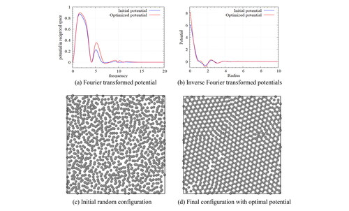
Graphical Abstract

Keywords:

• Self-assembly
• optimal design
• pair-wise isotropic potentials
• Fourier transform
• reciprocal space
• potential parameters
• low-coordinated crystals
• lattice structures

1. Introduction

A self-assembly is the process where individual elements form themselves into an ordered structure, and provides a novel way to design various substances for functional material properties. Self-assembly has been developed in various disciplines as a bottom-up manufacturing technique [1,2] that is used in various nanostructures with a high resolution. Polymers [3], proteins [4], DNA [5–7], and colloidal nanoparticles [2,8] can serve as relevant material building blocks for self-assembly due to their rich design space for mutual interactions, depending on size, shape, charge, and surface functionalization [9–11].

Many previous studies have made great progress in self-assembly by using a direct approach via intuition or exploration and an iterative approach in a trial-and-error fashion. The direct approach allows for empirical discoveries, but it is difficult to generalize from the terms of the target material design. On the other hand, in the iterative approach, materials are designed using optimization techniques aiming at the desired properties. Thus, the point of self-assembly is to determine and control the interactions with the target macroscopic properties of structures.

The classic inverse problem of designing a potential for targeted self-assembly focuses on pair-wise interactions in a ground state [12]. Specifically, we modulate the tunable parameters that determine an isotropic pair potential to design a targeted structure. This method produces many interesting results in the field of self-assembly. Research efforts discovered a pair potential to form various low-coordinated crystals (square [13], honeycomb [13,14], and Kagome [15]) using the iterative approach. Since the assembled structures are designed in a ground state, it is necessary to verify the stability under finite temperature conditions (e.g. a phonon spectrum). For the inverse design method, it is possible to generalize the approach with a machine learning technique [16]. Recently, an optimization method based on maximum likelihood machine learning [17] was applied to self-assembly problems. This optimization method, called relative entropy coarse graining [18,19], finds an inter-particle potential that produces the maximum likelihood of targeted configurations [20]. A successful relative entropy optimization was used for the self-assembly of various structures, such as Kagome and square lattices [21,22] and even more low-coordinated crystals such as truncated square and truncated hexagonal lattices [23,24], using an isotropic and repulsive pair potential.

The type of potential is not necessarily limited to repulsive pair potentials. There are studies to design a potential in the frequency domain for self-assembly of a target lattice by considering both attractive and repulsive forces. There are other studies where the ground state of periodic lattice structures corresponds to a pair potential where a Fourier transform is non-negative and vanishes beyond the specific limit of the wave number [25,26]. Edlund [27] introduced a method to produce the target lattice as a ground state using an energy spectrum. Furthermore, stable potentials to produce Kagome or diamond lattices were suggested by using the uncertainty principle [28]. Although the proposed potential produces the target lattice successfully as a ground state, it is not easy to apply the method extensively to various target lattices using the direct approach. Recently, a study was presented to design the potential in the frequency domain to produce the target lattice through an inverse approach [29].

In this article, through design optimization in reciprocal space and subsequent annealing simulation from a fluid state, we seek a more precise pair-wise potential for self-assembly that leads to the target lattice. We employ a Gaussian potential for robust design of various lattice structures to minimize information losses arising from continuous applications of Fourier and inverse Fourier transforms during the potential update process, utilizing a Fourier-Filtered Relative Entropy Minimization (FF-REM) formulation that minimizes the loss of information due to the Fourier transform, and facilitates fabricating the potential. It was possible to design a smooth and simple potential with less potential parameters for various target lattices by using the Gaussian potential in the reciprocal space. In addition, we can guarantee the target lattice to be the ground state by enforcing the potential to be zero at the reciprocal lattice points. Through this process based on the first order scheme of gradient-based optimization, we can obtain the precise potentials for various target lattices such as honeycomb and Kagome structures. Consequently, the convergence of the optimization can be significantly improved.

2 Potential for self-assembly

2.1. Pair-wise potentials in reciprocal space for a target lattice

We focus on a pair-wise isotropic potential in order to self-assemble targeted lattice structures. Edlund [27] suggested the direct approach to solve the inverse problem of designing isotropic potentials in a reciprocal space of the potential. Although this method is different from the problem we focus on since it aims to minimize the potential rather than minimize the entropy, the main idea of Edlund’s approach could help to effectively estimate the initial potential and to guide the direction of the designed potential imposing proper constraints on optimization iterations. Since gradient-based optimization finds a local minimum, the proper selection of initial design and constraints is important for successful design.

We consider a system of spherically symmetric particles in two-dimensional space. The configuration of the system can be expressed by the density defined using the pair correlation of particles. For a given configuration, $R_i,$ of a target structure, and with a set of potential parameters, $\mathbf{u},$ the total potential energy of the entire system is obtained using an isotropic pair-wise potential and its radial density of particles in either real space or reciprocal space (1) $$\begin{array}{c}V(R_i|\mathbf{u})=\pi \rho N{\int }_0^{\infty }dr·r{g}_i(r)V(r:\mathbf{u})\\ =\pi \rho N{\int }_0^{\infty }dk·k{\widehat{g}}_i(k)\widehat{V}(k:\mathbf{u}),\end{array}$$(1) where $g_i(r),V(r:\mathbf{u}),{\widehat{g}}_i(k),$ and $\widehat{V}(k:\mathbf{u})$ are the radial distribution function, the potential, the Fourier-transformed radial density, and the Fourier-transformed potential, respectively. Eq. (1)(1) $$\begin{array}{c}V(R_i|\mathbf{u})=\pi \rho N{\int }_0^{\infty }dr·r{g}_i(r)V(r:\mathbf{u})\\ =\pi \rho N{\int }_0^{\infty }dk·k{\widehat{g}}_i(k)\widehat{V}(k:\mathbf{u}),\end{array}$$(1) provides an important relation for designing the potential in a Fourier transformed space. The simulation uses potentials in real space, but design of the potentials is done in the frequency space. The designed potential using a Fourier (Hankel) transform of a radial distribution function guarantees a ground state for the target lattice.

To do that for designed potential V(r), the energy spectrum is positive for all frequency ranges, $\widehat{V}(k)\ge 0$ in a finite frequency domain has zeros only at frequencies coinciding with reciprocal lattice points, and $\widehat{V}(\left|G_i\right|)=0$ $(i=1,\dots ,n)$ where G_i of a Bravais lattice describes the target lattice. In this study, we propose an inverse design approach to potentials by applying the above rules to the optimization process for pair-wise potentials that self-assemble into a target lattice structure. Inverse design offers a great advantage in that it can design a potential for a complex target lattice structure by using an optimization algorithm without human estimation, but there are several challenges to be solved. One of them is that the simulation space and the design space are separated entirely. The design process is performed in the reciprocal space, whereas the response analysis is done in the physical space. Thus, it is necessary that the Fourier and inverse Fourier transforms of the potential are alternately performed in each step of t design updates. On the other hand, the limitation on the operational possibility of the Fourier transform is expressed by Heisenberg’s uncertainty principle [30] (2) $$\text{var}(f;x)·\text{var}(\widehat{f};k)\ge \frac{d^2}{16{\pi }^2},$$(2) where $\text{var}(f;x)$ indicates the variance of function f, and $\widehat{f}$ denotes the Fourier transform of f. The lower bound is achieved exactly in case f is a Gaussian function [31]. In this study, the pair-wise potential between particles is constructed as a Gaussian-based function in order to minimize the information loss that occurs outside the domain range during Fourier transformation or inverse Fourier transformation of the potential, which occur continuously in the optimization process.

Design of the potential in reciprocal space is beneficial in several aspects. It is possible to intentionally suppress the high-frequency region of the potential. Also, it guarantees a smooth and simple shape for potentials during the design optimization, unlike designing in real space. When designing a potential in real space, the number of sampling data varies for the calculation of ensemble average of the radial distribution function (RDF), depending on the distance between the particles. In the reciprocal space, however, uniform accuracy for the ensemble average is naturally achieved, which could reduce the computing time for the sampling of the RDF. Furthermore, the estimation of ansatz potential and the imposition of constraints on the reciprocal lattice points could lead to faster convergence and a preciser optimal potential in the optimization process.

2.2. Gaussian potential in reciprocal space

The Gaussian function is advantageous from the viewpoint of inverse design of a potential in reciprocal space since its variance does not depend on the mean. In this study, as described in the previous section, in order to utilize the advantage of the Gaussian function, we propose a potential form that includes superposition of the Gaussian function.

The following Gaussian potential provides a basis for precise design in reciprocal space (3) $$\widehat{V}(\eta ,\mathit{\sigma },\mathbf{p};k)=e^{-\eta k^2}\left(1-\sum _i^m{\alpha }_i{\widehat{V}}_i({\sigma }_i,p_i;k)\right),$$(3) (4) $${\widehat{V}}_i({\sigma }_i,p_i;k)=\frac{1}{{\mathit{\sigma }}_i\sqrt{2\pi }}{e}^{-\frac{{\left(k-p_i\right)}^2}{2{\sigma }_i^2}},$$(4) where ${\sigma }_i,p_i\in R^m$ construct each Gaussian function of Eq. (4)(4) $${\widehat{V}}_i({\sigma }_i,p_i;k)=\frac{1}{{\mathit{\sigma }}_i\sqrt{2\pi }}{e}^{-\frac{{\left(k-p_i\right)}^2}{2{\sigma }_i^2}},$$(4) . 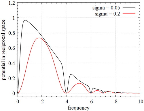The introduced Gaussian potential is superposition of m Gaussian functions; η yields an exponential decay and assists in suppressing a high-frequency region efficiently; and ${\sigma }_i$ smooths out the designed potential without losing the features of lattice structures in reciprocal space, as illustrated in Figure 1.

Figure 1. Smoothed Gaussian potential in reciprocal space; depending on the magnitude of smoothing parameter $\sigma ,$ appropriately regular Gaussian potential can be generated.

According to the principle introduced in the previous section, the Fourier transformed energy at the reciprocal lattice vector should vanish, which describes the target lattice structure. We can apply the principle introduced in the previous section to the Gaussian function as follows (5) $$V(G_i)=e^{-\eta G_i{}^2}\left(1-\sum _j{\alpha }_j{\widehat{V}}_i({\sigma }_j,G_j;G_i)\right)=0.$$(5)

Unlike σ_i and $p_i$ in Eq. (3)(3) $$\widehat{V}(\eta ,\mathit{\sigma },\mathbf{p};k)=e^{-\eta k^2}\left(1-\sum _i^m{\alpha }_i{\widehat{V}}_i({\sigma }_i,p_i;k)\right),$$(3) , α_i is determined by solving the following equations to force the potential to vanish at $G_i.$ $G_i\in \mathbf{p}$ is the reciprocal lattice point of a target Bravais lattice, which does not change during optimization. We choose η, σ_i, and $p_i$ as design variables for the optimization to design a potential. The system of equations in Eq. (5)(5) $$V(G_i)=e^{-\eta G_i{}^2}\left(1-\sum _j{\alpha }_j{\widehat{V}}_i({\sigma }_j,G_j;G_i)\right)=0.$$(5) should be solved at each step of the design update to determine an ${\alpha }_i$ that has implicit dependency on design variables.

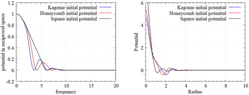
We designed pair-wise potentials as shown in Figure 2 for self-assembling a Bravais lattice of Kagome, honeycomb, and square lattices by direct estimation using the guideline introduced. The annealing simulations of randomly positioned particles build self-assembled particles that change from liquid to solid.

Figure 2. Designed potentials for various lattices-Fourier transformed potential (left), and Inverse Fourier-transformed potential (right); The potential in the original space increases drastically as reducing the radius. However, in reciprocal space, the shape of potential is more controllable.

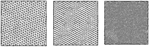
In Figure 3(left), observe that the Bravais lattice is well constructed, and three basis points are located at each Bravais lattice point, which is a characteristic of a Kagome lattice structure. Similarly, Figure 3(center) shows a configuration created with the designed potential for a honeycomb lattice. The honeycomb lattice has primitive vectors with a triangular Bravais lattice like the Kagome lattice, but consists of two basis points. The resulting configuration shows that the intended design is well reflected. On the other hand, the square lattice in Figure 3(right) is a Bravais lattice unlike Kagome and honeycomb lattice structures. We see that an appropriate square lattice is constructed only with the proposed approach. As the crystallization occurring at various locations propagates, we observe some defects in the regions where the square lattice is not properly formed, but most particles form a square lattice structure well. It is definitely possible that a simple lattice structure such as the Bravais lattice can be built by the potentials designed by estimation if they are followed by an introduced guideline using Gaussian form. However, it is almost impossible to design a potential that self-assembles with most of the complex lattices using the forward method that estimates potential by hand and that requires very sophisticated and difficult work. Therefore, we propose a methodology that can precisely design a potential that can self-assemble into a complex lattice structure through an iterative potential update by selecting the initial potential estimate through the above guideline and by using the gradient-based optimization technique.

Figure 3. Particle configurations by ansatz potentials for target Kagome(left), honeycomb(center), and square(right) lattices in annealing simulations. Such ansatz potentials form the Bravais lattices of the target structures directly. Since a gradient based optimization converges to a local minimum, an adequate choice of ansatz potentials is essential.

3 Design optimization method

3.1. Relative entropy minimization method

The main idea for applying the optimization technique is the pair-wise potential (the probability of self-assembling target lattice structure $\mathbf{R}$ for $\mathbf{u}$), so $P(\mathbf{u}|R)$ is selected as the objective function. Since probability $P(\mathbf{u}|R)$ cannot be obtained directly from molecular dynamic simulations, ‘likelihood’ could substitute for the problem of finding the maximum potential. The probabilities $P(\mathbf{u}|R)$ and $P(\mathbf{R}|u)$ are equivalent based on Bayes’ theorem by assuming that prior probability $P(\mathbf{u})$ is constant. In particular, the log likelihood corresponds to the configurational space functional called relative entropy [18,19]. Based on that approach, inter-particle interactions have been designed to maximize the relative entropy [22,29]. We employ the optimization algorithm outlined by Adorf [29], which derives FF-REM based on a maximum log likelihood approach. The log likelihood for the target configuration composed of discrete microstates $R_i$ $(i=1,\dots ,M)$ is expressed in the form of joint probability.

Consider the following Markov network to find a set of the potential’s parameter $\mathbf{u}$ that provides self-assembly for target structure configuration $R_i$ (6) $${\mathbf{u}}^{*}=\arg \max \left[P(\mathbf{u}|R_i)\right],i=1,2,\dots ,N$$(6)

This is a problem of finding the potential’s parameter set that exists with the highest probability, given the target configuration. Since it is very difficult to find a set with the highest a posteriori probability, we employ Bayes’ theorem (7) $$P(\mathbf{u}|R_i)=\frac{P(R_i|\mathbf{u})P(\mathbf{u})}{P(R_i)},$$(7) where $P(R_i)$ is independent of the potential’s parameters. We assume $P(\mathbf{u})$ has the same probability at each $\mathbf{u}.$ Then, we can reconstruct the problem to solve maximum likelihood. The original problem is changed to a problem of finding the potential’s parameters with the highest probability of the existence of the target configuration when the potential’s parameters are determined. The objective function for likelihood $P(R_i|\mathbf{u})$ can be expressed using the partition function as (8) $$P(R_i)=\frac{e^{-\beta V(R_i|\mathbf{u})}}{\sum _i{e}^{-\beta V(R_i|\mathbf{u})}},$$(8) where $P(R_i)$ is the probability of finding target configuration $R_i$ among all configurations consisting of potential energy V in an NVT ensemble, and $\mathbf{u}$ is the parameter set composed for potential $\widehat{V}$ in reciprocal space. Then, we define the joint probability (9) $$P(\Omega |\mathbf{u})=\prod _i^M\frac{1}{Z\left(\mathbf{u}\right)}{e}^{-\beta V(R_i|\mathbf{u})},$$(9) where Ω is all the M microstates sampled from the target distribution. If the configurations from the simulation with $\mathbf{u}$ approach the target configuration, the probability of Eq. (9)(9) $$P(\Omega |\mathbf{u})=\prod _i^M\frac{1}{Z\left(\mathbf{u}\right)}{e}^{-\beta V(R_i|\mathbf{u})},$$(9) approaches unity. Therefore, we define an optimization problem to find ${\mathbf{u}}^{*}$ as follows (10) $${\mathbf{u}}^{*}=\arg \max \left[\mathit{lnP}(\Omega |\mathbf{u})\right]=\arg \max L(\Omega |\mathbf{u}).$$(10)

Since P is always greater than 0, the maximum value of P in the above expression is the same as the maximum value of lnP, so it is defined as an optimization problem for lnP for convenience in the expression expansion. To perform gradient-based optimization, $\frac{dL}{d\mathbf{u}}$ is required where L is defined in Eq. (10)(10) $${\mathbf{u}}^{*}=\arg \max \left[\mathit{lnP}(\Omega |\mathbf{u})\right]=\arg \max L(\Omega |\mathbf{u}).$$(10) . (11) $$L=-\beta \sum _i^M\left\{V({\mathbf{R}}_i)-\mathit{MlnZ}(\theta )\right\}$$(11) where V is the same as in Eq. (1)(1) $$\begin{array}{c}V(R_i|\mathbf{u})=\pi \rho N{\int }_0^{\infty }dr·r{g}_i(r)V(r:\mathbf{u})\\ =\pi \rho N{\int }_0^{\infty }dk·k{\widehat{g}}_i(k)\widehat{V}(k:\mathbf{u}),\end{array}$$(1) when expressed using the radial distribution function, g(k) in two-dimensional space, so $\frac{dV}{d\mathbf{u}}$ and $\frac{d(\mathit{lnZ})}{d\mathbf{u}}$ can be written as (12) $$\frac{dV}{d\mathbf{u}}=2\pi \rho N{\int }_0^{\infty }dk·k{\widehat{g}}_i(k)\frac{d\widehat{V}(k:\mathbf{u})}{d\mathbf{u}}$$(12) (13) $$\frac{d(\mathit{lnZ})}{d\mathbf{u}}=-\beta \sum _i^{\Gamma }\frac{1}{Z}{e}^{-\beta V({\mathbf{R}}_i)}\frac{dV}{d\mathbf{u}}$$(13) where, Γ means the number of all microstates that can be made with u. Also, the radial distribution function, $〈g(k){〉}_{*},$ and u in target lattice structure $〈g(k){〉}_{\mathbf{u}}$ are expressed as (14) $$〈g(k){〉}_{*}=\frac{1}{M}\sum _i^M{g}_i(k)$$(14) (15) $$〈g(k){〉}_{\mathbf{u}}=\sum _i^{\Gamma }\frac{e^{-\beta V({\mathbf{R}}_i)}}{Z(\mathbf{u})}{g}_i(k)$$(15)

Using the above relationship, design sensitivity $\frac{dL}{d\mathbf{u}}$ of the relative entropy for the NVT ensemble in two-dimensional space can be calculated as follows (16) $$\frac{dL}{d\mathbf{u}}=C{\int }_0^{\infty }dk·k\left[{〈\widehat{g}(k)〉}_{\mathbf{u}}-{〈\widehat{g}(k)〉}_{*}\right]{\nabla }_{\mathbf{u}}\widehat{V}(\mathbf{u};k),$$(16) where $C=2\mathit{\text{MβπρN}}$ is a trivial constant that is independent of design variables; ${〈\widehat{g}(k)〉}_{\mathbf{u}}$ represents a Fourier-transformed RDF obtained by simulation, with the potential composed of the current design parameters, and ${〈\widehat{g}(k)〉}_{*}$ is the Fourier transformed RDF obtained in the target configuration. ${\nabla }_{\mathbf{u}}\widehat{V}(\mathbf{u})$ indicates the design sensitivity of a potential in reciprocal space. Since the Gaussian potential is designed by $\mathbf{u}$ composed of η, σ_i, and $p_i,$ the design sensitivity of Gaussian potential $\widehat{V}$ with respect to η, σ_i, and $p_i$ $(i=1,..,m)$ is expressed as (17) $$\frac{d}{d\eta }\widehat{V}(k)=-k^2{e}^{-\eta k^2}\left(1-\sum _i{\alpha }_i{\widehat{V}}_i({\sigma }_i,p_i;k)\right),$$(17) (18) $$\frac{d}{d{\sigma }_l}\widehat{V}(k)=-e^{-\eta k^2}\left(\sum _i\frac{d{\alpha }_i}{d{\sigma }_l}{\widehat{V}}_i\left({\sigma }_i,p_i;k\right)+{\alpha }_l\frac{d{\widehat{V}}_l\left({\sigma }_l,p_l;k\right)}{d{\sigma }_l}\right),$$(18) and (19) $$\frac{d}{d{p}_l}\widehat{V}\left(k\right)=-e^{-\eta k^2}\left(\sum _i\frac{d{\alpha }_i}{d{p}_l}{\widehat{V}}_i\left({\sigma }_i,p_i;k\right)+{\alpha }_l\frac{d{\widehat{V}}_l\left({\sigma }_l,p_l;k\right)}{d{p}_l}\right).$$(19) in which $d{\alpha }_i/d{\sigma }_l\mathrm{ }$ and $d{\alpha }_i/d{p}_l\mathrm{ }$ are obtained from the differentiation of Eq. (5)(5) $$V(G_i)=e^{-\eta G_i{}^2}\left(1-\sum _j{\alpha }_j{\widehat{V}}_i({\sigma }_j,G_j;G_i)\right)=0.$$(5) (20) $$\sum _i\frac{d{\alpha }_i}{d{\sigma }_l}{\widehat{V}}_i({\sigma }_i,G_i;G_j)+{\alpha }_l\frac{d{\widehat{V}}_l({\sigma }_l,G_l;G_j)}{d{\sigma }_l}=0,$$(20) and (21) $$\sum _i\frac{d{\alpha }_i}{d{p}_l}{\widehat{V}}_i({\sigma }_i,G_i;G_j)+{\alpha }_l\frac{d{\widehat{V}}_l({\sigma }_l,G_l;G_j)}{d{p}_l}=0.$$(21)

If j = l, Eq. (21)(21) $$\sum _i\frac{d{\alpha }_i}{d{p}_l}{\widehat{V}}_i({\sigma }_i,G_i;G_j)+{\alpha }_l\frac{d{\widehat{V}}_l({\sigma }_l,G_l;G_j)}{d{p}_l}=0.$$(21) can be rewritten using the relation $d{\widehat{V}}_l({\sigma }_l,G_l;G_l)/d{p}_l=0$ as follows (22) $$\sum _i\left[\frac{d{\alpha }_i}{d{p}_l}{\widehat{V}}_i({\sigma }_i,G_i;G_l)+{\alpha }_i\frac{d{\widehat{V}}_i({\sigma }_i,G_i;G_l)}{d{p}_l}\right]=0.$$(22) $d{\widehat{V}}_i({\sigma }_i,p_i;k)/d{\sigma }_l\mathrm{ }$ and $d{\widehat{V}}_i({\sigma }_i,p_i;k)/d{p}_l\mathrm{ }$ are obtained from the differentiation of Eq. (4)(4) $${\widehat{V}}_i({\sigma }_i,p_i;k)=\frac{1}{{\mathit{\sigma }}_i\sqrt{2\pi }}{e}^{-\frac{{\left(k-p_i\right)}^2}{2{\sigma }_i^2}},$$(4) , (23) $$\frac{\partial }{\partial {\sigma }_l}{\widehat{V}}_l\left({\sigma }_l,p_l;k\right)=\frac{1}{{\sigma }_l^2\sqrt{2\pi }}\left[\frac{{\left(k-p_l\right)}^2}{{\sigma }_l^2}-1\right]e^{-\frac{{\left(k-p_l\right)}^2}{2{\sigma }_l^2}},$$(23) and (24) $$\frac{\partial }{\partial p_l}{\widehat{V}}_l\left({\sigma }_l,p_l;k\right)=\frac{\left(k-p_l\right)}{{\sigma }_l^3\sqrt{2\pi }}{e}^{-\frac{{\left(k-p_l\right)}^2}{2{\sigma }_l^2}}.$$(24)

The formulation introduced above can be applied to any parameterized potential designed for self-assembly, and can be extended to multi-component systems in the same way. Each radial distribution function of a component can be used to design potentials of many component combinations. There are numerous interaction potentials that allow particles to form a specific target lattice structure in a ground state. Among many designed interaction potentials, the reason for focusing on simplification of the potential form is to be useful when realizing an experiment.

3.2. Formulation of design optimization

We consider the optimization problem with inequality constraints, (25) $$\min -L(\Omega |\mathbf{u})\hspace{1em}s.t.\hspace{1em}{C}_i(\mathbf{u})\le 0,i=1,2,\dots ,m,$$(25) where $\mathbf{u}$ denotes the design variables of η, $\mathit{sigm}{a}_i,$ and $p_i,$ which form a Gaussian potential function. $L(\Omega |\mathbf{u})$ is the log likelihood of finding the target configuration. $C_i(\mathbf{u})$ is used as a constraint on forming an appropriate potential to target a Bravais lattice by satisfying $\widehat{V}(\left|G_i\right|)=0.$ However, $\widehat{V}(\left|G_i\right|)=0$ was converted into inequality constraints for smooth design variation with a small tolerance, ε.

We solve optimization problem Eq. (25)(25) $$\min -L(\Omega |\mathbf{u})\hspace{1em}s.t.\hspace{1em}{C}_i(\mathbf{u})\le 0,i=1,2,\dots ,m,$$(25) for self-assembly using a classical molecular dynamics module, LAMMPS [32], on a high-performance computer cluster, the IBM PowerSystem S822LC. LAMMPS performs parallel processing using an MPI library and a spatial-decomposition technique for the simulation domain. In this study, we modified the LAMMPS code to be used with an optimization module. After calculating the RDF in the LAMMPS simulation, the part calculating design sensitivity is inserted into pair.cpp. Then, the updated potential is stored in a tabulated potential by reflecting the values of the calculated sensitivity and the constraint. The RDF for the targeted lattice is generated from in-house MD simulation code where the particles are pinned to the target lattice positions and connected to the nearest neighbor particles with a harmonic potential. The spring constant is chosen such that the particles are not broken during the simulations generating the RDF that includes sufficiently sharp target features. The LAMMPS simulation can be performed repeatedly using LAMMPS input script commands. The optimal design is determined by sufficiently iterating the simulations with the updated potential.

4 Numerical results and discussions

4.1. Honeycomb lattice

MD simulations were performed for 1,058 particles in a simulation box satisfying a density of 0.770 in a honeycomb lattice for an NVT ensemble. A thermal equilibrium simulation was performed such that the particles could move freely at a sufficiently high temperature. The annealing process was simulated over one million time steps from $k_{B}T=3.0ϵ$ to $k_{B}T=1.0ϵ$ with a step size of 0.01. 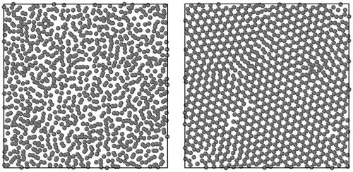Then, the particles were equilibrated over one million time steps at $k_{B}T=1.0ϵ$ to calculate the RDF. After a sufficient amount of time had passed, the final configuration of the particles in the last time step was chosen as the initial configuration for the optimization process, as shown in Figure 4(left). After the updates of potential parameters were sufficiently accomplished to obtain the optimally designed potential, the lattice configuration through the annealing simulation was obtained as shown in Figure 4(right). Since crystallization occurs everywhere simultaneously, some defects are found here and there, as seen in Figure 4(right), due to kinetic trapping in the annealing simulation.

Figure 4. Particle configurations for the self-assembly of honeycomb lattice at the initial time step (left) and the final time step with the optimal potential (right); With the obtained optimal potential, the particles are randomly distributed at initial simulation, and then are cooled down steadily until sufficient crystallization occurs.

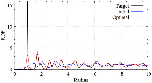
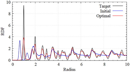
To evaluate the optimization results quantitatively, RDFs were obtained from the ideal target potential, the initially guessed potential, and the optimally designed potential seen in Figure 5. To obtain the RDF of the target lattice, a simulation was performed to maintain an appropriate temperature by placing the particles precisely at the target lattice points. Interactions are defined using harmonic potentials that act between the closest particles. The RDF changes according to either the equilibrated temperature or the coefficients of the harmonic potential without a position change in the coordinate shells. The corresponding values for the temperature and the coefficients were selected to obtain the target RDF. Through the design optimization, the optimal parameters for self-assembly of the honeycomb lattice were obtained. The obtained RDF was almost the same as the RDF for the target lattice. The peak height of the first coordinate shell differed significantly from that of the target lattice, which was caused by the several defects.

Figure 5. Comparison of RDFs for honeycomb lattice with target(black), initial(blue) and optimal(red) potentials; The obtained RDF of optimal potential is almost the same as that of the target lattice. The peak height of the first coordinate shell differs significantly from that of the target lattice, which is caused from the several defects but the heights of peak can be changed with temperature conditions.

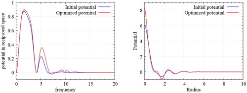
Figure 6(left) shows the Fourier-transformed potential in reciprocal space as the design space. Note that considerable changes occurred through the optimization evolution. In particular, a frequency range of 5–10 is a highly sensitive region for optimal design of the potential due to its significant influence on fluctuation of the potential in real space.

Figure 6. Designed potential for honeycomb Lattice – Fourier transformed potential(left) and inverse Fourier transformed potentials(right); The frequency range of 5–10 is highly sensitive for the optimal design of potential due to its significant influence on the fluctuation of potential in the real space.

The history of the optimization process is shown in Figure 7. Since the objective function is relative entropy, it is very difficult to calculate the relative entropy directly through the MD simulations. Therefore, the following measure is defined to observe the approximate history of the optimization process: (26) $${\varphi }^2=\int {\left(g_{*}(r)-g_T(r)\right)}^{2}dr,$$(26) which is a fitness measure and indicates the difference between the target and the designed RDFs. Some fluctuations are observed in the optimization history, but the RDF from the optimal design is markedly decreased, compared with the RDF from the initial design.

Figure 7. Optimization history for honeycomb structure; The history of difference between the target and the designed RDFs in Eq. (22)(22) $$\sum _i\left[\frac{d{\alpha }_i}{d{p}_l}{\widehat{V}}_i({\sigma }_i,G_i;G_l)+{\alpha }_i\frac{d{\widehat{V}}_i({\sigma }_i,G_i;G_l)}{d{p}_l}\right]=0.$$(22) is plotted as we perform the simulations. Some fluctuations are observed but eventually the RDF by the optimal design is markedly decreased.

4.2. Kagome lattice

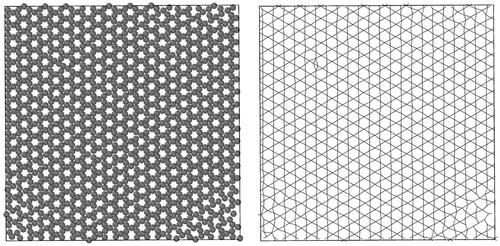
For the design of a Kagome lattice, the initial potential is estimated in a different way from the honeycomb lattice. The approximate potential guide in the previous section is considered together with the reciprocal lattice vectors. Thus, the constraints and the initial potential are also different from those of the honeycomb lattice design. All the other conditions are the same as those for the honeycomb lattice. Figure 8(left) shows the self-assembled configuration after performing annealing simulations using the optimally designed potential. Figure 8(right) shows a configuration net where the center of the particle is connected to that of adjacent particles for easy visualization of the lattice. We observed that some defects occur in some corner sites, as shown in Figure 8(right). However, most of the particles form the Kagome lattice successfully.

Figure 8. Particle configurations in Kagome lattice – Final configuration with optimal potential (left), Configuration net for visualization (right); The configuration net shows the connectivity of adjacent particles for the easy visualization of lattice structure.

The RDFs obtained from the ideal target potential, the initially guessed potential, and the optimally designed potential are shown in Figure 9. Through the design optimization, the optimal potential parameters for self-assembly of the Kagome lattice are obtained. Note that the obtained RDF is almost the same as the RDF for the target lattice. Compared to the target lattice, the peak of the coordinate shell is slightly different, but the position of the coordinate shell is almost identical. This difference can be controlled by the temperature in the simulations.

Figure 9. Comparison of RDFs for Kagome lattice; Compared to the target lattice, the peak of coordinate shell is slightly different. However, its position is almost identical and the difference can be reduced by controlling the temperature of simulations.

Figure 10(a) shows the Fourier transformed potential that satisfies the relation $V(\left|\mathbf{G}\right|)=0$ in reciprocal space (Figure 10b). Slight changes are observed through the optimization evolution. In the optimization history shown in Figure 11, some fluctuations in the fitness measure of Eq. (26)(26) $${\varphi }^2=\int {\left(g_{*}(r)-g_T(r)\right)}^{2}dr,$$(26) are observed, but the overall tendency is decreasing.

Figure 10. Designed potential for Kagome Lattice – Fourier transformed potential (left), Inverse Fourier transformed potentials (right).

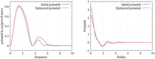
Figure 11. Optimization history for Kagome structure; Some fluctuations of the fitness measure in Eq. (26)(26) $${\varphi }^2=\int {\left(g_{*}(r)-g_T(r)\right)}^{2}dr,$$(26) are observed but the overall tendency is decreasing.

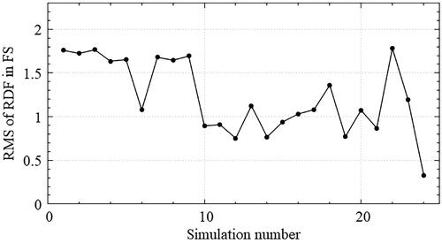
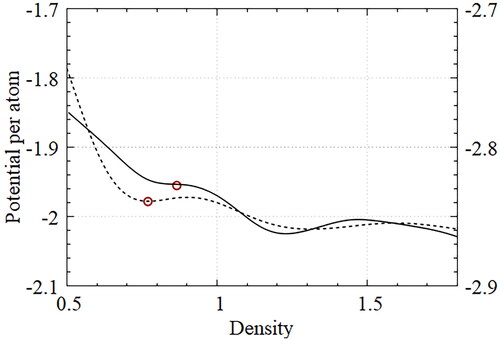
Figure 12. Energy per atom with designed potentials for the honeycomb lattice (dotted) and the Kagome lattice (solid) according to density variations; Each potential was designed at a specified density (red circles).

The initial particle configuration was obtained through thermally equilibrated NVT simulations at high temperature. The ground state configuration was obtained through annealing simulations in which the final temperature was lowered to one-third of the initial temperature through a quenching process. A thermally equilibrated NVT simulation was performed over one million time steps at a sufficiently low temperature to sample the data and calculate the RDF. We discuss the impact of density on self-assembly performance with the optimized potential. All the other simulation conditions, except molar density changing from 0.5 to 1.8, were the same as those used in the optimization process.

Figure 12 shows the potential energy per atom with the designed potentials for the honeycomb lattice (dotted line) and the Kagome lattice (solid line) according to variations in density. The potentials in the figure were averaged at each density from five identical simulations. The appropriate density ranges from 0.7 to 0.9 such that the designed potentials produce the target lattices of honeycomb and Kagome lattices successfully. The red circles indicate the densities used for both optimization processes. Observe that lower energies were achieved in the higher density regions for both optimal potentials. Both potentials create triangular lattices in the density range of 1.18 to 1.5. The square lattices appear at a slightly higher density range than the triangular lattice.

As shown in Figure 13, the optimized potentials for honeycomb and Kagome structures could self-assemble various unsuspected lattices depending on the simulation density. The optimal potential for the Kagome lattice could lead to a striped pattern in a low-density range, as shown in Figure 13(left). However, the optimal potential for the honeycomb lattice creates a triangular lattice with twice the unit length in the low-density region, as shown in Figure 13(right). Since we consider both attractive and repulsive forces, it is likely to self-assemble the structure as a competitor, such as a triangular lattice or a square lattice.

Figure 13. Self-assembled configuration with a designed potential at low density condition – Kagome lattice (left, density 0.66), honeycomb lattice (bottom, density 0.54); In case the density deviates to a certain extent, a stripe pattern can be obtained for Kagome lattice (left) and a triangular lattice with twice unit length for honeycomb lattice (right).

The target lattice is well constructed near a density where simulations for the optimization were performed. If the density deviates to a certain extent, however, a completely different striped pattern can be obtained, especially in the potential for the Kagome lattice, as shown in Figure 13. This phenomenon implies that the designed potential may not possess sufficient stability. The self-assembled lattice could be varying depending on the density. The target lattice may not be self-assembled accurately, depending on the density, since the designed potential cannot completely eliminate various competitors occurring at the density ranges other than the density where the optimization is actually performed [24]. In this study, since we enforced the potential at the reciprocal lattice point of the target lattice to be zero, other types of lattices can also be in the ground state. To prevent the competitive lattices from creating a ground state, we need other conditions such as small perturbation of the potential [27]. In the Kagome lattice, narrow distinctions between highly related competitors such as stripe patterns are revealed more clearly at other densities. Therefore, completely removing competitive alternative structures is an important condition in order to improve stability and to self-assemble the target lattice in various density ranges. In addition, if the designed potential has multiple wells, a tunneling effect could interfere with the stable settlement of particles. Further research is necessary to avoid the designed potential having multiple wells.

The potentials for the Kagome and honeycomb lattices obtained from inverse design are slightly different from those proposed by Edlund [28], but show almost complete self-assembly processes for the target lattices. The potential designed through the inverse approach rather than the forward approach can also accurately create various complex lattices. It can be confirmed that the difference between the initial and optimal potentials is small if designed by the Relative Entropy Minimization method [22]. The optimization problem is non-convex, and since there exist many design parameters, the shape of the initial potential could not be significantly changed. Using a Gaussian potential in reciprocal space and a constraint that enforces the target lattice to be in the ground state, however, we obtain a general form with much fewer potential parameters that can be applied to various lattices and provide better convergence behavior.

5 Conclusions

We demonstrated that by using pair-wise isotropic potentials designed by a gradient-based optimization method in reciprocal space, it is possible to produce various non-Bravais lattices such as Kagome and honeycomb structures. To efficiently remove unnecessary noise and to guide the potential to the target lattice in a ground state configuration based on the ansatz potential and constraints, design optimization of a potential’s parameters is performed in reciprocal space. A Gaussian potential in reciprocal space that is the lower bound of Heisenburg’s inequality was chosen for minimal loss of information due to Fourier and inverse Fourier transforms during design updates. We modified the LAMMPS code, embedding the derived design-sensitivity formula to be used with an optimization module, and successfully designed the potentials for various lattice structures, such as the square, triangle, Kagome, and honeycomb. The designed potential may not possess sufficient stability (depending on the density) since it cannot sufficiently eliminate various competitive alternative structures outside the density range where optimization is actually accomplished.

Notes on contributors

Jae-Hyun Kim received his B.S., M.S. and Ph.D. in Naval Architecture and Ocean Engineering from Seoul National University, Korea. He is now working for Samsung Electronics in the field of molecular dynamic simulations. His research interests include molecular dynamic simulation, computational mechanics, and novel material design.

Seonho Cho is a professor at Seoul National University in Korea. He graduated from the department of naval architecture at Seoul National University with a B.S. and M.S. degrees. In 1998, he was awarded a Ph.D. degree in the area of design optimization from the department of mechanical engineering at the University of Iowa in U.S.A. His specialization includes design sensitivity analysis and optimization, nano mechanics, molecular dynamic simulations, and other novel computational methods.

Data availability

The data that support the findings of this study are available from the corresponding author upon reasonable request.

Disclosure statement

No potential conflict of interest was reported by the authors.

References

- Grzelczak M, Vermant J, Furst EM, et al. Directed self-assembly of nanoparticles. ACS Nano. 2010;4(7):3591–3605.
- Menger FM, Seredyuk VA, Apkarian RP, et al. Colloidal assemblies of branched geminis studied by cryo-etch-HRSEM. High-resolution scanning electron microscopy. J Am Chem Soc. 2002;124(42):12408–12409.
- Bates FS, Hillmyer MA, Lodge TP, et al. Multiblock polymers: panacea or pandora’s box? Science. 2012;336(6080):434–440.
- Dill KA, MacCallum JL. The protein-folding problem, 50 years on. Science. 2012;338(6110):1042–1046.
- Lee YC, Moon JY. Introduction to bionanotechnology: biological self-assembly. Singapore: Springer; 2020. p. 79–92.
- Pinheiro AV, Han D, Shih WM, et al. Challenges and opportunities for structural DNA nanotechnology. Nat Nanotechnol. 2011;6(12):763–772.
- Zhang Q, Jiang Q, Li N, et al. DNA origami as an in vivo drug delivery vehicle for cancer therapy. ACS Nano. 2014;8(7):6633–6643.
- Lehn JM. Supramolecular chemistry. Science. 1993;260(5115):1762–1763.
- Breen TL, Tien J, Oliver SR, et al. Design and self-assembly of open, regular, 3D mesostructures. Science. 1999;284(5416):948–951.
- Isaacs L, Chin DN, Bowden N, et al. Self‐assembling systems on scales from nanometers to millimeters: design and discovery. Vol. 4, Perspectives in supramolecular chemistry: supramolecular materials and technologies; 1999. p. 1–46.
- Sherman ZM, Howard MP, Lindquist BA, et al. Inverse methods for design of soft materials. J Chem Phys. 2020;152(14):140902.
- Torquato S. Inverse optimization techniques for targeted self-assembly. Soft Matter. 2009;5(6):1157–1173.
- Marcotte, Stillinger FH, Torquato S. Unusual ground states via monotonic convex pair potentials. J Chem Phys. 2011;134(16):164105.
- Rechtsman MC, Stillinger FH, Torquato S. Optimized interactions for targeted self-assembly: application to a honeycomb lattice. Phys Rev Lett. 2005;95(22):228301.
- Jain A, Errington JR, Truskett TM. Dimensionality and design of isotropic interactions that stabilize honeycomb, square, simple cubic, and diamond lattices. Phys. Rev. X. 2014;4(3):031049.
- Sanchez-Lengeling B, Aspuru-Guzik A. Inverse molecular design using machine learning: generative models for matter engineering. Science. 2018;361(6400):360–365.
- Barber D. Bayesian reasoning and machine learning. Cambridge University Press; 2012.
- Shell MS. The relative entropy is fundamental to multiscale and inverse thermodynamic problems. J Chem Phys. 2008;129(14):144108.
- Chaimovich A, Shell MS. Coarse-graining errors and numerical optimization using a relative entropy framework. J Chem Phys. 2011;134(9):094112.
- Piñeros WD, Lindquist BA, Jadrich RB, et al. Inverse design of multicomponent assemblies. J Chem Phys. 2018;148(10):104509.
- Piñeros WD, Baldea M, Truskett TM. Designing convex repulsive pair potentials that favor assembly of kagome and snub square lattices. J Chem Phys. 2016;145(5):054901.
- Lindquist BA, Jadrich RB, Truskett TM. Communication: inverse design for self-assembly via on-the-fly optimization. J Chem Phys. 2016;145(11):111101.
- Jadrich R, Lindquist B, Truskett T. Probabilistic inverse design for self-assembling materials. J Chem Phys. 2017;146(18):184103.
- Piñeros WD, Truskett TM. Designing pairwise interactions that stabilize open crystals: truncated square and truncated hexagonal lattices. J Chem Phys. 2017;146(14):144501.
- Sütõ A. Crystalline ground states for classical particles. Phys Rev Lett. 2005;95(26):265501.
- Uche OU, Stillinger FH, Torquato S. Constraints on collective density variables: two dimensions. Phys. Rev. E. 2004;70(4):046122.
- Edlund E, Lindgren O, Jacobi MN. Designing isotropic interactions for self-assembly of complex lattices. Phys Rev Lett. 2011;107(8):085503.
- Edlund E, Lindgren O, Jacobi MN. Using the uncertainty principle to design simple interactions for targeted self-assembly. J Chem Phys. 2013;139(2):024107.
- Adorf CS, Antonaglia J, Dshemuchadse J, et al. Inverse design of simple pair potentials for the self-assembly of complex structures. J Chem Phys. 2018;149(20):204102.
- Folland GB, Sitaram A. The uncertainty principle: a mathematical survey. J Fourier Anal Appl. 1997;3(3):207–238.
- Borowko M, editor. Computational methods in surface and colloid science. CRC Press; 2019. ISBN 0429524838
- Plimpton S. Fast parallel algorithms for short-range molecular dynamics. Comput Phys. 1995;117(1):1–19.