Uncertainty propagation and sensitivity analysis in composite manufacturing cost estimation: ALPHA-framework and cost tool development

Abstract

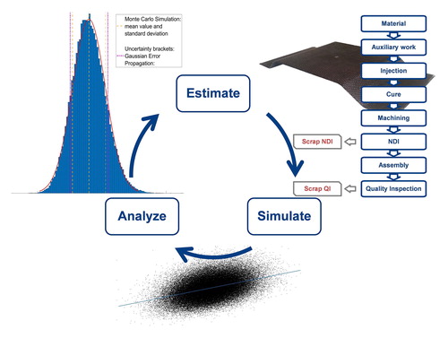
The presented ALPHA cost tool is a novel highly flexible bottom-up parametric hybrid cost estimation framework. It combines the benefits of both methods with the aim of providing cost information during all product development phases. The software offers full transparency to the user and advanced two-level uncertainty management to not only understand any project’s cost structure but also aid to identify its cost driving parameters. The implementation of sensitivity analysis makes the intrinsic uncertainty inevitable embedded in cost estimation become graspable. Gaussian error propagation offers direct feedback without extra calculation time while classic Monte Carlo Simulation gives detailed insight through post estimation analysis. From the vast number of commercially available or self-developed cost tools many probably already incorporate uncertainty measures similar to those proposed here. But this article shows both the potential of the additionally obtainable information from uncertainty propagation and demonstrates a way of integrating these risk considerations into a self-developed cost tool.

GRAPHICAL ABSTRACT

Keywords:

• Cost estimation
• sensitivity analysis
• Monte Carlo simulation
• composite processing
• aerospace manufacturing

1. Introduction

The strength of composites is their superior mechanical properties paired with unmatched lightweight potential and a high degree of design freedom. But their main weakness is the complex and labor-intensive manufacturing process combined with high raw material costs.

Rising financial pressure, also in traditionally less concerned industries like aerospace or racing applications, increases the need for sufficient cost estimation and control methods suitable to composite manufacturing industry. Reliable cost estimation is the foundation for successful business operation, which makes it a core feature in streamlining production efficiency. Not only correct bidding depends on cost estimation, but also all design and production decisions need to be economically evaluated with the help of cost estimation. Unfortunately, as the name estimation already indicates this process is always afflicted with a varying degree of uncertainty. This uncertainty can either come from errors in estimating the individual input parameters or from unforeseeable economic changes [1–3].

It is therefore extremely advantageous to not only obtain a reasonable estimation, but to also know the likelihood of a specific result and the expected deviation based on model input uncertainty. Uncertainty analysis helps to comprehend the impact of these errors and it allows identification of system critical parameters, the so-called cost drivers. The recognition of these values is important to the estimation as it tells which parameters to focus upon.

In this article the authors will discuss cost estimation together with suitable methods for uncertainty management and will present their concept of what they consider an ideal cost tool for composite aerospace manufacturing. A case study will demonstrate the application of the developed ALPHA software estimation tool and the importance of uncertainty management within cost estimation. Additionally, this article also aims to provide a guideline on the development of a cost tool, the possible trade-offs that need to be made and other important things that need to be considered.

2. ALPHA - hybrid cost estimation framework

2.1. Cost estimation methods

In general, all cost estimation approaches can be classified according to one of the following three basic methods (analogous, parametric and bottom-up cost estimation) or as a combination of them. While the distinction into these three methods is commonly enough, Niazi, et al. [4] provide a more detailed approach for classification of cost estimation models. Here only the fundamental principles for cost estimation will be discussed. Further and more detailed information on cost estimation especially for composite aerospace manufacturing can be found in [4–7].

2.1.1. Analogous cost estimation

The concept of analogous cost estimation follows the idea of using stored historic case knowledge to establish an estimation of the current project. The selection of the known past cases is governed by similarity. This can be done either rather simplistic by just selecting the most similar case and directly take the cost values from it or by establishing more complex similarity comparison methods that generate estimates based on multiple cases and their according level of resemblance. When applicable the analogous method provides a fast and easy way to obtain reliable estimation. The downside is the need to correctly identify the required similar case and to adequately rate the economic impact of case deviations [8–12].

2.1.2. Parametric cost estimation

The idea of parametric estimation is to statically analyze historic cases in order to establish mathematic correlations between project parameters and project costs. Once found, these so-called cost estimation relationships (CERs) allow for rapid estimation as long as the current case is within the CER’s historic data range. Finding this correlation can either happen manually, normally leading to causal relationships or by applying for example neural networks with the downside of generating black-box systems [13–17].

2.1.3. Bottom-up cost estimation

While the two methods above relay on evaluation of historic knowledge the third method, bottom-up, works by decomposing the whole project into smaller and easy to estimate elements. These elements can either be work steps, activities or design features. After generating individual estimates for each element, these are summed up to form the full estimate of the project. This procedure provides highest flexibility of all methods and the freedom of independence from historic cases. But it also requires a large amount of design details and process understanding by the estimator and takes the most time to conduct [18–25].

2.1.4. Method comparison

Parametric and Analogous estimation technique are especially suitable for fast and easy estimations with limited amount details known, as long as sufficient applicable historic case knowledge is available. If unavailable or if a more detailed estimation is needed, the Bottom-up technique is the best option. It is also the most flexible method as it is not restricted by historic cases, but on the downside, it needs the highest amount of user input and known design details. A quantitative comparison of the different techniques and their strengths and weaknesses is shown in Figure 1.

Figure 1. Quantitative comparison of the basic estimation methods and the ALPHA hybrid concept [26].

In cost estimation practice different methods are used for different settings and models often are a combination of two or all three basic methods, see Hueber et al. [6] for more details.

2.2. Bottom-up-parametric hybrid

For the development of our cost estimation model, ALPHA, we decided on a Bottom-up- parametric hybrid approach. The idea was to combine the flexibility and applicability to new technologies of the bottom-up method with the early design stage capabilities of parametric. The aim was to develop a single estimation platform that allows cost estimation throughout all product development phases. This idea is displayed in Figure 2 in combination with a cost development curve taken from Duverlie and Castelain’s study [11]. As can be seen it is very important to establish cost control in the development process as early as possible [2]. In the beginning it is essential to get rough numbers with a minimum of effort and details needed. As development progresses the influence of smaller details become more central and the estimation is required to allow for those to affect the outcome. This is when the higher details of bottom-up become preferable.

Figure 2. Time vs. cost commitment with methods; based on Duverlie and Castelain [11].

In ALPHA this method combination was realized with a work step-based bottom-up basic framework. The desired estimate is built up from single elements for every work step required in the desired manufacturing chain. This allows for fully customizable process chains and maximum estimation flexibility. It gives the cost engineer absolute control over the estimation process without constraints, while providing him with templates to increase speed and reproducibility of the estimation. Each element is then estimated either by classic engineering cost build-up or by using a parametric equation for this work step, depending on the available data and the desired estimation detail. Alternatively or additionally to these individual step elements a full-scale parametric model can be integrated into the estimation chain. This then allows the complete top-down estimation of the part. The whole program was designed to be easily adaptable to changing requirements and new element templates can be generated and implemented rapidly. This concept can be seen in Figure 3 showing the available estimation methods and their combination in ALPHA. [26]

Figure 3. The concept and estimation methods in ALPHA.

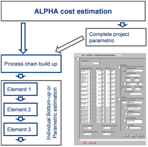
Figure 4. Exemplary scatter plots for the function $y=k·x_1+k·x_2+k·x_3+k·x_4$ with increasing influence from $x_1\mathrm{ }$to $x_4.$ The uniform distributions indicate low sensitivity, while emerging patterns indicate increasing sensitivity [38, 39].

By combining these two systems in one framework, it is possible for example to expand the full-scale parametric estimation with additional work steps, which are not covered in the parametric equation. This could be an additional curing cycle or that the part is to be integrated into a larger assembly with further production steps. But the most important benefit is the possibility for seamless transition between rapid and detailed estimation which makes it ideal for application in all development stages. The full level parametric model was developed in parallel by our project partner first as a standalone tool and later intended as an extension module to be implemented within the ALPHA framework [27–30].

The ALPHA tool was developed specifically with single processes or parts in mind. In comparison to full system solutions this reduces program complexity and helps implementation in early stages where it aims to support designers in their decision process. Full system estimation is of more interest on the strategic level and needs special experts to operate, while ALPHA is created as a tool for day to day use at the practical engineering level. But the developed methodology could be applied to full system estimation as well, if needed.

Several reasons exist, why it might be beneficial to self-develop a cost tool in comparison to purchasing a commercially available solution. Frist only the self-development allows the freedom to choose the best fitting method combination for one’s desired application. Second it offers the chance to generate the exact needed process chains and process steps or to allow the flexibility to adapt and expand the capabilities on demand. Another big advantage is the achievable transparency of the estimation as all used equations and data are accessible. In ALPHA the wish for clarity led to all equations being presented to the user while entering the input values. We see this crucial as unknown mathematics will lead to a black-box system, which reduces estimator’s confidence in the system.

The biggest downside is probably the needed development time and resources, but then one has to be aware that also the commercial tool will need adaption time, effort to learn the tool and resources to adjust the databases to the individual needs.

3. Sensitivity and uncertainty

Cost estimation is inherently affected by uncertainty originating for from different sources. First are economic uncertainties arising from unpredictable changes on the market, like energy costs, fuel prices, etc. or unforeseeable changes in exchange rates, taxes or inflation. The second source is engineering errors resulting in wrong assumptions of required input quantities, falsely calculated production times or overlooked complications. In addition to this a model always has to incorporate simplifications in order to stay comprehensible which might cause errors if not correctly accounted for. [1,3,31–34]

The goal of sensitivity analysis is to investigate the influence of the individual input parameters of a model to the overall model output [35–37]. It can generally be distinguished into two types: local and global sensitivity analysis. In the first one the influence of every input value on the result is calculated for a specific value of the input parameter. But this result is then only valid within a small range around this defined value. In contrast to that the global analysis uses the statistical distribution for the input parameter to analyze the influence over the full variable space [35,36,38–41].

3.1. Uncertainty propagation, Monte Carlo simulation and sensitivity indices

In the ALPHA cost estimation tool, a two-level uncertainty management was implemented. Simple error propagation provides immediate feedback on the to be expected uncertainty brackets, while Monte Carlo simulation takes additional calculation time before allowing insight into probabilistic cost distribution. For the ALPHA cost estimation tool, a two-level uncertainty analysis was intended. The first level should be able to immediately give a rough overview of to be expected effects of set uncertainties.

3.1.1. Gaussian error propagation

For this purpose, the first-order second-moment or Gaussian error propagation (GEP) method described in Equation (1)(1) $${\sigma }_f\approx \sqrt{\sum _{i=0}^n{\left(\frac{\partial y}{\partial x_i}V\mathit{ar}\left(x_i\right)\right)}^2}$$(1) was used. But for GEP to be applicable it is necessary that the full model is expressible as an analytical equation or function of all input variables and all input variables have to be assumed to be uncorrelated and normal distributed. But this is acceptable as in common practice this would be necessary anyway as it would by extremely difficult for estimation problems to obtain any information on the correlation between the inputs or to establish higher order distributions [42,43].

Besides the mentioned limitations GEP provides an easy to implement method that requires little recurring calculation efforts. Only the establishment of the local differentiations can be time consuming. In ALPHA this was solved by calculating them once at implementation and recording them within the program. Only if an equation is altered or a new one introduced to the system, e.g. when a new module is added, then on its first execution ALPHA will automatically calculate the new needed local differentiations and again save them for future use. This ensures that the time-consuming generation is only done when needed and, in the meantime, GEP is able to provide direct feedback without noticeable calculation time. (1) $${\sigma }_f\approx \sqrt{\sum _{i=0}^n{\left(\frac{\partial y}{\partial x_i}V\mathit{ar}\left(x_i\right)\right)}^2}$$(1) where $\frac{\partial y}{\partial x_i}\text{ is the }$partial differentiation of function for input ${\mathrm{x}}_{\mathrm{i}},$ ${\sigma }_f\text{ is the }$result standard deviation, $\mathit{Var}\left(x_i\right)$ is the variation of input $x_i, \mathrm{and}$ $x_i\text{ is the }$input parameter.

Although factor correlations are normally neglected, approaches to model them still exist in the literature. For example [3,44] propose the use of a Bayesian network, [31] suggest including correlations in the Monte Carlo Simulation and [45] advised to combine strongly correlated variables into one.

While the error propagation can be calculated directly during the estimation process, the more intensive sensitivity analysis needs to be conducted once finished. For this second phase of the uncertainty management a Monte Carlo approach with global sensitivity analysis was chosen [31,32,34,46].

3.1.2. Sigma normalized derivative

The sigma normalized derivative is the simplest sensitivity index. It is generated by normalizing the derivative of the function $y$ versus the input parameter $x_i$ with the standard deviations of the input and output. This ensures that the indices are all normalized to 1 making them independent from the value of original input and that the quadratic sum of all $S_{x_i}^{\sigma }$ equals 1, which is necessary for meaningful parameter-ranking [39]. (2) $$S_{x_i}^{\sigma }=\mathrm{ }\frac{{\sigma }_{x_i}}{{\sigma }_y}\frac{\partial y}{\partial x_i}$$(2) where $S_{x_i}^{\sigma }$ is the sigma normalized derivative for input x_i, σ_y is the standard deviation of  function, ${\sigma }_{x_i} \mathit{is} \mathit{the}$ standard deviation of input x_i and $\frac{\partial y}{\partial x_i}$ is the partial difference of function for input $x_i.$

3.1.3. Monte Carlo simulation, scatter plots and linear regression

In various variations Monte Carlo simulation (MCS) is the widely used method for risk and uncertainty measurements. It works on the premise that for all inputs a normal distribution with an expected mean value and standard deviation is known or determinable. Based on these input distributions a pseudo random sample, called the Monte Carlo matrix (MCM), is created. It contains a row or line vector for every individual input parameter. Its size is specified by the number N defining the amount of random numbers for every parameter. The choice of N highly influences the quality of the MCS, but calculation efforts for sensitivity indices also increases drastically by the factor 2*N or N², depending on the used calculation method [39,47].

Scatter plots, as explained in Figure 4, are a graphical method to identify influence of input factors [39]. To help visualize, the point clouds are often combined with regression fittings. Based on the mostly linear nature of the model and the shape of the clouds, basic linear regression was chosen in this work.

Although the scatter plots provide very neat visual information, one could wish for a single number per parameter to rate its influence. The most common method for this to achieve is to try and fit a linear regression in the form of Equation (2)(2) $$S_{x_i}^{\sigma }=\mathrm{ }\frac{{\sigma }_{x_i}}{{\sigma }_y}\frac{\partial y}{\partial x_i}$$(2) onto the data. The two coefficients $b_0$ and $b_{x_j}$ should be determined by the method of least-square computation [39]. (3) $$y\left(i\right)=b_0+\sum _{j=1}^n{b}_{x_j}{x}_j^{\left(i\right)}$$(3) $\mathrm{where} y$ is the regression function, $b_0 \text{is the first coefficient}$ and $b_{\mathit{xj}}$ is the second coefficient.

Now the standardized regression coefficients (Equation (4)(4) $${\beta }_{\mathit{xi}}=\frac{b_{\mathit{xi}}·{\sigma }_{\mathit{xi}}}{{\sigma }_Y},$$(4) ) can be calculated. It provides a reliable measurement of the sensitivity to the individual input and the linearity of the whole model, which can be assessed by the sum of squares for all $b_{x_j}.$ For a linear model it equals 1 and less for any percentage of non-linearity. (4) $${\beta }_{\mathit{xi}}=\frac{b_{\mathit{xi}}·{\sigma }_{\mathit{xi}}}{{\sigma }_Y},$$(4) where ${\beta }_{\mathit{xi}}$ is the standardized regression coefficient, $b_{\mathit{xi}}$ is the regression coefficient of input $x_i,$${\sigma }_{\mathit{xi}}$ is the standard deviation of input $x_i, \mathrm{and} {\sigma }_Y$ is the standard deviation of the function.

The biggest disadvantage of the before introduced sigma normalized derivative is that it only evaluates around the distribution midpoints. The linear regression coefficient and the following variance-based indices on the other hand are established using the full space of the input factors. But their fidelity requires the Monte Carlo sample number to be large enough [39].

3.1.4. Variance based methods (first- and total-order sensitivity index)

Another important class of sensitivity index is those of the variance-based types, of which the first-order or main effect and the total-order sensitivity index are the most used. While very useful, all variance-based indices suffer from the drawback of relying for the variance to capture the total uncertainty behavior of the input variables [38].

The first order sensitivity index, defined as shown in Equation (5)(5) $$S_i=\frac{V_{x_i}\left(E_{x_{\sim i}}\left(y|x_i\right)\right)}{V\left(y\right)},$$(5) , represents the direct contribution of the individual parameter to the output variance, which is why it is also referred to as main effect. It is best suitable for ranking of the factors, when the factor interaction can be considered non-relevant [37–39]. (5) $$S_i=\frac{V_{x_i}\left(E_{x_{\sim i}}\left(y|x_i\right)\right)}{V\left(y\right)},$$(5) where $S_i$ is the first order sensitivity index of input $x_i,$ V is the variance, E is the expected value and $x_{\sim i}$ is the all input factors but except the i-th factor.

The first order index captures only the direct influence of the factor. In order to determine interaction between parameters higher order indices are required. The second order index can detect interaction between parameter pairs, the third order these of input triplets, and so on. From this principle Sobol [41] introduced the total effect index often referred to as Sobol indices [47,48]. They imply the full effect of a factor, including its direct contribution plus all its interactions with the other factors and are defined through Equations (6(6) $$S_{T1}=\mathrm{ }{S}_1+S_{12}+S_{13}+S_{123},$$(6) ,7) (7) $$S_{\mathit{Ti}}=\frac{E_{x_{\sim i}}\left(V_{x_i}\left(y|x_{\sim i}\right)\right)}{V\left(y\right)},$$(7) [36]. S₁ is the first order index calculated as shown in Equation (5)(5) $$S_i=\frac{V_{x_i}\left(E_{x_{\sim i}}\left(y|x_i\right)\right)}{V\left(y\right)},$$(5) for model parameter 1, while S_1j are second and higher order indices for the interaction between the factors 1 and j [37–39]. (6) $$S_{T1}=\mathrm{ }{S}_1+S_{12}+S_{13}+S_{123},$$(6) where $S_{T1}$ is the total order sensitivity index of input $x_1,$ S₁ is the main effect of input $x_1$ and S_1j are the second and higher order effects of input $x_1$ and $x_j.$

The Sobol indices are especially suitable for parameter screening; those parameters whose total effect are zero can be considered non-influential. While full calculation of them can be tedious for large models, suitable estimators for both first- and total-order indices exist for approximation [49]. (7) $$S_{\mathit{Ti}}=\frac{E_{x_{\sim i}}\left(V_{x_i}\left(y|x_{\sim i}\right)\right)}{V\left(y\right)},$$(7) where $S_{\mathit{Ti}}$ is the total order sensitivity index of input $x_i,$ V is the variance, E is the expected value and$x_{\sim i}$ is the all input factors but except the i-th factor.

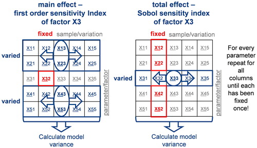
To calculate the main effect, the parameter is fixed at one of its variations, before calculating the model’s variance from the remaining MCM. This procedure is repeated for every variation of the parameter existing in the original MCM. For calculating the total effect, the procedure is similar with only one difference. All but the one parameter is fixed before calculating the variance. The concept of these basic calculation principles for the two sensitivity indices is shown in Figure 5 [39].

Figure 5. Concept of the calculation of first and total order sensitivity index.

It is the scope of much research to find improved calculation algorithms for these and similar sensitivity indices in order to make sensitivity analysis applicable to ever more complex problems [39,47,50]. One of these approaches would be the use of Fourier transformation (FAST) for the calculation of the sensitivity indices [37].

4. Sensitivity analysis on composite manufacturing cost estimation

4.1. Case study description

The sensitivity analysis was performed on the cost estimation of an resin transfer moulding (RTM) composite part manufactured to industrial standards. The estimated process chain shown in Figure 6 consists of the raw material, preparation of the tool and preform placement. The actual RTM process takes place in a press with a two-component injection unit used to infuse the preform with resin. After curing the part is demolded and put to machining for edge trim before non-destructive inspection (NDI) for quality insurance is performed. The production is finished with some assembly and final quality inspection. In both quality steps scrap is detected and its costs are assessed based on the so far invested production resources.

Figure 6. Assumed part production chain and surveyed input variables with their statistic range.

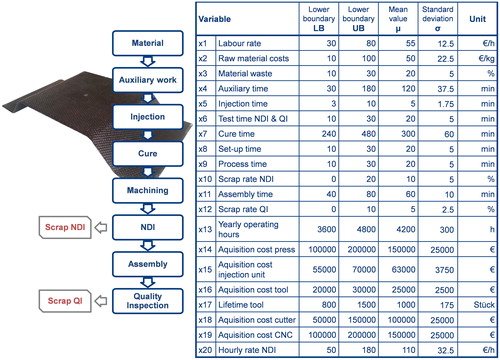
For every parameter listed in Figure 6(a) most likely value was determined and used in the ALPHA cost estimation. Further plausible lower (LB) and upper (UB) boundaries for these estimation values were defined and integrated for the tools error propagation. To fit the MCS a standard distribution was assumed in a way that the mean value µ coincides with the most likely value, while standard deviation σ was set to be one quarter of the difference of UB to LB, resulting in 95, 45% of the distributions values to be within the UB/LB boundaries. All other parameters were set to fixed values, first to keep evaluation efforts manageable and second because it was assessed that these values can either be estimated very accurately or are given values from financing or controlling department.

For the sensitivity simulation the MCM was filled with pseudorandom numbers according to the statistical definitions in Figure 6. The convergence was tested for different matrix sizes. A larger matrix size provides a higher resolution, but the calculation time and memory demand also dramatically increase with it.

4.2. Results

4.2.1. Cost distribution

Performing the cost estimation in ALPHA provided two outcomes: first the estimated product’s manufacturing time and cost and second the uncertainty brackets for both values obtained through Gaussian Error Propagation for the whole project and for each individual work step. Figure 7 shows the contribution of each estimated work step together with the expected uncertainty generated via uncertainty propagation. The high auxiliary costs are typical for composite parts as in this case they cover tool preparation, demolding and preforming time. Material costs, curing and quality costs are also to be expected significant contributors to composite’s production costs.

Figure 7. Estimated manufacturing cost distribution per work step, with propagated uncertainty and type wise distribution of case study composite part.

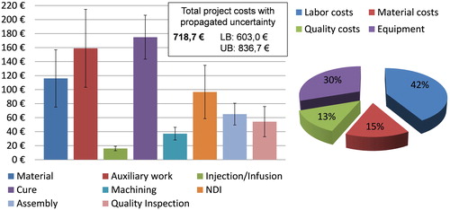
Besides the per work step distribution a cost split-up into labor, equipment and material costs can also be seen in Figure 7 together with the estimated total project costs and size of the Gaussian uncertainty brackets. It shows the characteristically high contribution of labor costs to overall manufacturing costs of a composite part.

4.2.2. Monte Carlo analysis

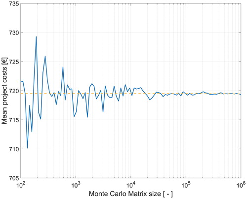
By performing a MCS additional information can be gained once the estimation is set up. In order to choose the right size or resolution of the MCM a convergence study was conducted whose results are displayed in Figure 8. The graphic shows the convergence of the mean value of the project costs over the size of the MCM, which is basically the number of considered pseudo random values per input parameter. Therefore, at a total of 100 different size points, logarithmically distributed between 1x10² and 1x10⁶, three iterations were created, analyzed and their mean value was also calculated. The calculation of three iterations with subsequent averaging was done to compensate for outliers at the low size range of the study. With larger matrix size the outliers start to be balanced out within the matrix themselves. From the graphic can be seen that the deviation quickly recedes and from 5x10⁴ on is negligibly small. Based on this finding all further evaluations in this article was conducted using a MCM size of 1x10⁵ as a good compromise of resolution and computational effort [31,35].

Figure 8. Convergence of the mean project costs over the size of the Monte Carlo Matrix.

The analysis allows the establishment of the cost distribution function that is shown in Figure 9. It can be seen that the directly estimated uncertainty is in very tight correlation with the obtained standard deviation from the MCS. The uncertainty brackets are only a little bit wider, covering around 74% of expected cases, while 68% are within the standard deviation. But one must be aware, that this correlation is depending on the model’s linearity and it only works well in this case due to the linear character of the cost estimation.

Figure 9. Cost probability distribution from Monte Carlo Simulation using 100 thousand variations. The mean value equals the result obtained from estimation in ALPHA.

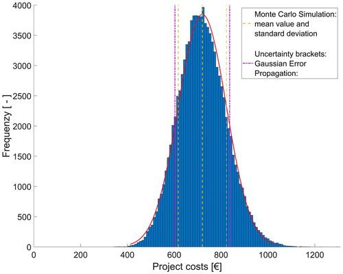
The charm of the graphic evaluation in Figure 9 and the MCS in general is simple to implement while providing large amount of additional insight. Especially it cannot only show an error range, but also provides the distribution of the expected manufacturing cost.

Further the transformation into the cumulative probability function shown in Figure 10 is also pivotal. This visualization allows for graphical risk analysis and enables the cost estimator trade-offs between expected risk and possible profit. It shows directly the probability or likeliness for the production cost to be below a certain value, helping in the definition of offerings. Especially providing feedback on the risk involved with specific offering prices or discounts.

Figure 10. Cumulative probability function for the project costs.

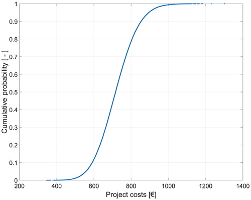
For example, in this case the probability for the project costs remain below 800€ are about 80% and there is a more or less than 100% chance that the costs will not exceed 1000€. This means that being able to offer/sell the part for more than 1000€ nearly certainly provides a revenue (not considering overheads).

4.2.3. Scatter plots, sensitivity indices and parameter ranking

The information generated by the Monte Carlo analysis was further used to characterize the model’s behavior in dependences of the individual input parameters in detail. Therefore, for each of the 20 investigated input variables scatter plots were generated, visualizing their influence on the outcome. From the scatter diagrams the linear regression and the linear regression coefficient was calculated by the method of least squares. Further the data was used to establish the first- and total-order sensitivity indices and compare them to the sigma normalized derivatives mentioned in Table 1 [47].

Table 1. Calculated sensitivity indices for the evaluated parameters.

Variable		Sigma normalized derivative ${(S}_{x_i}^{\sigma }$)	Linear regression coefficient (${\beta }_{x_i}$)	First order sensitivity index ($S_{x_i}$)	Total effect sensitivity index ${(S}_{T_i}$)
1	Labour rate	0.656121	0.606712	0.431766	0.379532
2	Raw material costs	0.460469	0.413159	0.213036	0.174096
3	Material waste	0.042636	0.038735	0.001829	0.001795
4	Auxiliary time	0.564673	0.506853	0.320108	0.267606
5	Injection time	0.033605	0.032078	0.001127	0.000934
6	Test time NDI and QI	0.151121	0.149399	0.022992	0.024113
7	Cure time	0.340682	0.305892	0.116250	0.095069
8	Set-up time	0.056340	0.049275	0.003190	0.002717
9	Process time	0.049234	0.043795	0.002435	0.002015
10	Scrap rate NDI	0.341165	0.023704	0.120908	0.000642
11	Assembly time	0.093799	0.091027	0.008886	0.009349
12	Scrap rate QI	0.184044	0.182675	0.034277	0.035522
13	Yearly operating hours	−0.029030	0.028194	0.000874	0.000745
14	Acquisition cost press	0.059922	0.059237	0.003628	0.003057
15	Acquisition cost injection unit	0.000106	0.001183	0.000000	0.000000
16	Acquisition cost tool	0.029135	0.021836	0.000906	0.000768
17	Lifetime tool	−0.050986	0.056560	0.003533	0.002911
18	Acquisition cost cutter	0.002820	0.000316	0.000008	0.000007
19	Acquisition cost CNC	0.005640	0.009915	0.000032	0.000027
20	Hourly rate NDI	0.123171	0.123085	0.015387	0.016404

In general, the four most influential parameters shown in Figure 11 are of no surprise, when looking at the cost distribution in Figure 7. With 42% labor costs are by far the most dominant cost factor, which is primarily defined by the labor rate and secondly by the required times for labor intensive work steps. The high influence of the auxiliary time is somewhat specific to this case study and derives from a production characteristic of this part. Due to the sealing configuration tool preparation requires unusual long time, while the flat preform geometry requires no preforming step. In a more typical process, the auxiliary time would probably be replaced by preforming time in the list of most influential parameters. And although the material costs in Figure 7 contain several additional positions, the raw material costs in Figure 11 are their main contributor. The cure time is also a well-known cost driver for composite parts with long curing times. But even though the found cost drivers were not unsuspected being able to mathematically qualify and correctly rate them in all estimations is highly valuable information to every cost estimator.

Figure 11. Scatter plots of the four most influential parameters.

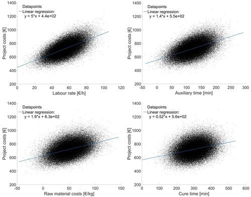
In direct comparison of the different sensitivity indices (see Table 1) a change of ranks can be found for three parameter pairs. Cure time and scrap rate are one of them. While the linear regression and sigma normalized derivatives consider cure time more important than scrap rate, the first order and the total effect sensitivity index both see scrap rate before the cure time. This is because the sensitivity indices and especially the higher order indices are better suited for non-linear correlations and both scrap rates are the two non-linear factors in this case study. But generally, one can see that the model is highly linear as the first Sobol (total effect) index, first-order (main effect) sensitivity index and linear regression coefficient are all in close correlation to each other [47]. Second the sum of ${{\beta }_{\mathit{xi}}}_{}^2$ (quadrat sum of the linear regression coefficient) equals 0.9839 indicating 98% linearity [39].

The two negative factors for the sigma normalized derivative (X₁₃ and X₁₇) originate in the indirect proportionality of these two factors to the model output causing the local derivatives to be negative for these two parameters.

5. Discussion

The emphasis of article is on cost tools in general and their key factors that need to be considered in a cost tool in order to maximize its usefulness. The focus was not on the strength or capability of an individual cost tool, nor any specific application of one, although one was presented as an example.

Composite production is on the verge from ‘garage shop manufacturing’ to full grown automated industry with the need to adopt typical standard management processes. Two of which are cost estimation and uncertainty management. This article links for the first-time composite production cost estimation with uncertainty propagation and risk management.

5.1. Requirements and benefits for cost tool

In order to achieve the desired benefit a cost tool has to fulfil several often-contradicting requirements. But when correctly designed the use of a standardized cost tool can provide heightened reproducibility, fidelity and homogenization of the performed cost estimations. It further allows the seamless incorporation of knowledge systems and databases and can be used for integrated multiattribute cost-versus-optimizations. Figure 12 summarizes the key attributes considered by the authors for a good cost estimation tool in this article. While being a relatively simple image, the novelty and charm of Figure 12 is that it shows at one glance all needed aspects of a cost tool paired with the encountered trade-offs.

Figure 12. Perceived attributes for an ideal cost estimation tool; blue elements pose possible competing interests.

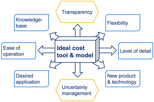
Transparency and uncertainty management are perceived as primary and non-contradicting factors. Transparency for the user is absolutely necessary in order to avoid a black box feeling and ensure the estimators trust in the tool and its capability. It also decreases the risk of estimation errors caused by not fully understanding the software. Risk and error considerations are necessary simply because cost estimation can never be an exact procedure and awareness of this intrinsic uncertainty is essential.

Based on the needs and purpose of the model careful trade-offs might be necessary for the other six attributes. Tailoring it to a specific application makes it less complex and easier to use, but also reduces flexibility and its ability to be applied to new manufacturing technologies or products. The same applies to the wished level of detail. The more detailed the more complex the model gets, the less user-friendly it can become.

5.2. Cost tool development: roadmap and guideline

The biggest benefit of a self-developed cost tool is that it can be designed specifically to the requirement needs. This allows for the principle ‘as complex as needed, as simple as possible’ while still providing every desired information and required functionality. Commercial software on the other hand often is either not designed for the specific application or has far too extended capabilities making it complex to operate. Additionally, the software must not be believed to be directly fully operational, but instead extensive training, establishment of datasets and adaptations are still necessary.

Commercial software therefore often has an adjustment slider to adapt underlying equations and estimation principles to different applications and companies. But identifying the right setting of such an adjustment parameter can prove difficult and in our experience, allows the estimation to virtually take on any value desired. Full estimation flexibility and transparency is often only achievable with a self-developed system. When choosing to develop a custom-built cost estimation software one first has to carefully consider the desired capabilities, functionality and the planned phase of application as described in the following or depicted in Figure 13.

Figure 13. Development steps for an uncertainty-controlled cost estimation tool.

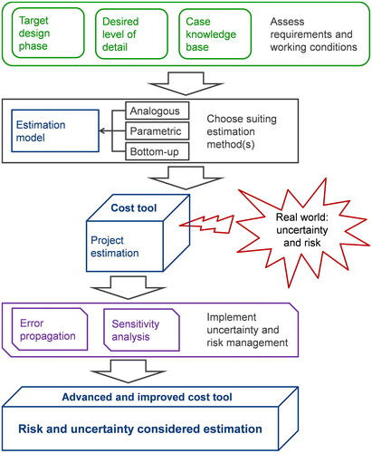
At the beginning the fundamental requirements of the tool need to be set by answering among others the following questions: For which phase of the product development is the cost tool intended for? Should it provide a quick and rough estimation at little detail during the early stages or is a more detailed estimation required to balance small design details or production optimizations?

Then the product portfolio has to be analyzed thoroughly in respect to its diversity, available case knowledge and the possibility to establish such knowledge. Available knowledge bases or the implementation of knowledge systems can help drastically reduce estimation times, but one has to be careful to not unknowingly extrapolate beyond the knowledge base’s data range. For very different products it might be more difficult to find a common cost driver, but chances are that still some can be found and the model might just need additional input or correction factors.

Depending on the defined requirements and the character and availability of historic case knowledge the most suitable estimation method or a combination of them must be chosen as foundation of the model. Analogous and parametric estimation are more suitable for the early design stages with little known details, while bottom-up becomes more favorable in later stages where it can provide more information. A general classification of the methods was given in Section 2.1 and Figure 1 and a detailed overview of concepts and models for the composite aerospace industry can be found in [4–6].

But without additional sensitivity error handling any estimation tool lacks the capability to take into account estimation uncertainty or risk. Typically, these would be uncertainties from estimating model input parameters like material usage or labor times or external risks from for example possible price changes. Additional sensitivity analysis allows the statistic evaluation of the model and the identification of estimation critical parameters. As already discussed before, the authors think this is a crucial aspect in cost estimation and consider uncertainty awareness absolutely necessary for every estimation process. The most basic technique would be simple error propagation like the first order second moment (or Gaussian) method used in the ALPHA cost tool. Its main benefit, besides the easy implementation, being the extremely low needed calculation power allowing for immediate feedback to the estimator even during the model set up. On the downside it is only capable of returning simple error values which represent a probabilistic boundary for the eventual outcome and its fidelity is depending on the model’s linearity. For mostly linear models though theses error brackets correspond very well with the standard deviation obtained from the far more time-consuming MCS. The MCS is probably the most common method for sensitivity analysis in order to generate information of the model’s sensitivity to changes of the individual input parameters. At the same time, it allows the establishment of a cost distribution function which enables refined financial risk and potential assessment.

5.3. Encountered limitations

In the establishment of the presented cost tool and moreover during this work the following limitations were encountered. Some of which are inevitable for cost estimation while others just had to be accepted for the time being:

• In absence of better knowledge any correlation between the individual input parameters were neglected and all parameters were considered as independent.

• The underlying cost estimation is subject to typical simplifications and possible estimation errors.

• All model values and their distributions were chosen to the best of the authors knowledge and belief, but mis judgement in cost estimation can never be fully eliminated.

• For the sensitivity analysis only a basic Monte Carlo method with brute force calculation of the indices was implemented. More advanced techniques could lead to similar results while consuming significantly less calculation time.

• Due to missing real-life industry data the intended parametrizes for the individual work steps could not be established, although the software is fully designed to incorporate and facilitate them.

• The simple error propagation and sensitivity indices (sigma normalized derivative, linear regression coefficient and to some degree the first order sensitivity index) only work reliable for linear models and quickly loose fidelity for increasing non-linearity.

• A detailed benchmark and method comparison, although highly interesting, was impossible as it would have required additional comparable cost estimation that was unavailable to us.

Although present in this development, some of the limitations could be overcome with additional development time or in different application context. In the case of an existing knowledge base statistic tests could be applied to uncover potential correlations between inputs which then can be included in the model to consider the dependencies. The transfer of estimation parametrizes between industries or even different companies would always be dangerous and either needs careful checking and probably adaptation or completely new development would be necessary. The used Monte Carlo simulation is not only the most common method but is also often used as benchmark to test improved calculation methods which could be implemented in a different realization. Upon implementation a model can easily be tested for its linearity and to check its suitability for the simple uncertainty methods or the need of advanced methods. Generally, should a cost tool never be considered finished, but should always be subject to continuous improvement through experience.

6. Conclusion

In this article one possible concept for a cost estimation tool capable to cover the full spectrum of aerospace composite part development was presented. The novelty of the ALPHA approach lies mainly in the specific method combination and the new application of these established methods to cost estimation in the composite manufacturing environment. Especially the use of the Gaussian error propagation provides a very good and instantly available uncertainty feedback. Its limitation to linear systems being rather uncritical as cost relations are mainly linear or close-to-linear in nature. Further it was shown that the establishment and implementation of uncertainty and risk management into an existing cost estimation tool is rather simple, while afterwards proving to be a very important and helpful improvement to the final estimation. This work presents the basic steps of cost estimation, what to consider in an estimation tool and simple measurements for uncertainty control together with a short example and guideline on cost tool development. In conclusion neglecting uncertainty largely reduces the value of any cost estimation. Especially as a single output promises a false sense of certainty which is against the nature of any cost estimation process. Only implementation of an uncertainty measurement leads to a cost tool capable of providing the essential information needed for successful business operation.

Acknowledgment

The authors kindly thank the Christian Doppler Forschungsgesellschaft for their administrative support.

Disclosure statement

No potential conflict of interest was reported by the authors.

Additional information

Funding

The authors kindly thank the Bundesministerium für Digitalisierung und Wirtschaftsstandort and the FACC Operations GmbH for funding this research.

References

- Bertisen J, Davis GA. Bias and error in mine project capital cost estimation. Eng Economist. 2008;53:118–139.
- Cheung JMW, Scanlan JP, Wiseall SS. An aerospace component cost modelling study for value driven design. In: Roy R, Shehab E, editors. Proceedings of the 1st CIRP Industrial product-service systems (IPS2) Conference; Bedford: Cranfield University, 2009.
- Khodakarami V, Abdi A. Project cost risk analysis: a Bayesian networks approach for modeling dependencies between cost items. Int J Project Manage. 2014;32:1233–1245.
- Niazi A, Dai JS, Balabani S, et al. Product cost estimation: technique classification and methodology review. J Manuf Sci Eng. 2006;128:563.
- Curran R, Raghunathan S, Price M. Review of aerospace engineering cost modelling: the genetic causal approach. Prog Aerosp Sci. 2004;40:487–534.
- Hueber C, Horejsi K, Schledjewski R. Review of cost estimation: methods and models for aerospace composite manufacturing. Adv Manuf Polym Compos Sci. 2016;2:26–37.
- NASA. NASA cost estimating handbook. Washington, DC: National Aeronautics and Space Administration; 2008.
- Esawi AMK, Ashby MF. Cost estimates to guide pre-selection of processes. Mater Des. 2003;24:605–616.
- Feldman P, Shtub A. Model for cost estimation in a finite-capacity environment. Int J Prod Res. 2006;44:305–327.
- Rush C, Roy R. Expert judgement in cost estimating: modelling the reasoning process. CERA. 2001;9:271–284.
- Duverlie P, Castelain JM. Cost estimation during design Step: Parametric Method versus Case Based Reasoning Method. Int J Adv Manuf Technol. 1999;15:895–906.
- Rehman S, Guenov MD. A methodology for modelling manufacturing costs at conceptual design. Comput Ind Eng. 1998;35:623–626.
- Roy R. Cost engineering: why, what and how? [Internet]. Cranfield, UK: Decision Engineering Report (DEG) Series; 2003. Available from: https://dspace.lib.cranfield.ac.uk/handle/1826/64. Accessed date 24 February 2014.
- International Society of Parametric Analysts. Parametric estimating handbook [Internet]. 4th ed. Vienna, VA 22180; 2008. Available from: http://www.galorath.com/images/uploads/ISPA_PEH_4th_ed_Final.pdf.
- Gutowski TG, Henderson RM, Shipp C. Manufacturing costs for advanced composites aerospace parts. SAMPE J. 1991;27:37–43.
- Ye J, Zhang B, Qi H. Cost estimates to guide manufacturing of composite waved beam. Mater Des. 2009;30:452–458.
- Neoh ET. Adaptive framework for estimating Fabrication Time [dissertation]. Cambridge (MA): Massachusetts Institute of Technology; 1995.
- Karbhari VM, Jones SK. Activity-based costing and management in the composites product realization process. Int J Mater Prod Technol. 1992;7:232–244.
- Spedding TA, Sun GQ. Application of discrete event simulation to the activity based costing of manufacturing systems. Int J Prod Econ. 1999;58:289–301.
- Ou-Yang C, Lin TS. Developing an integrated framework for feature-based early manufacturing cost estimation. Int J Adv Manuf Technol. 1997;13:618–629.
- Witik RA, Payet J, Michaud V, et al. Assessing the life cycle costs and environmental performance of lightweight materials in automobile applications. Compos Part A Appl Sci Manuf. 2011;42:1694–1709.
- Jung J-Y. Manufacturing cost estimation for machined parts based on manufacturing features. J Intell Manuf. 2002;13:227–238.
- Schubel PJ. Cost modelling in polymer composite applications: case study – analysis of existing and automated manufacturing processes for a large wind turbine blade. Compos Part B-Eng. 2012;43:953–960.
- Schubel PJ. Technical cost modelling for a generic 45-m wind turbine blade produced by vacuum infusion (VI). Renew Energy. 2010;35:183–189.
- Pantelakis SG, Katsiropoulos CV, Labeas GN, et al. A concept to optimize quality and cost in thermoplastic composite components applied to the production of helicopter canopies. Compos Part A Appl Sci Manuf. 2009;40:595–606.
- Hueber C, Schledjewski R. Holistic concept for efficient composite manufacturing. SAMPE J. 2018;54:34–39.
- Horejsi K, Noisternig J, Koch O, et al. Process selection optimization of CFRP parts in the aerospace industry. ECCM15 - 15th European Conference on Composite Materials; 2012 June 26–30; Venice, Italy.
- Hueber C, Horejsi K, Schledjewski R. Bottom-up Parametric Hybrid Cost Estimation for composite aerospace production. Proceedings of the 17th European Conference on Composite Materials (ECCM 17); 2016 September 19–20; München.
- Horejsi K, Koch O, Noisternig J, et al. Cost-based process selection in early design stages for composite aircraft parts. SETEC. 12:8439–8445.
- Horejsi K, Schledjewski R, Noisternig J, et al. Cost-saving potentials for CFRP parts in early design stages. Proceedings of the 19th International Conference on Composite Materials; 2013 July 28-August 2; Montreal, Canada, p. 8439–8445.
- Touran A, Wiser E. Monte Carlo technique with correlated random variables. J Constr Eng Manage (ASCE). 1992;118:258–272.
- Chou J-S, Yang I-T, Chong WK. Probabilistic simulation for developing likelihood distribution of engineering project cost. Autom Constr. 2009;18:570–577.
- Kleijnen JPC, Helton JC. Statistical analyses of scatterplots to identify important factors in large-scale simulations, 1: Review and comparison of techniques. Reliab Eng Syst Saf. 1999;65:147–185.
- Lee SH, Chen W. A comparative study of uncertainty propagation methods for black-box-type problems. Struct Multidisc Optim. 2009;37:239–253.
- Sobol′ IM. Global sensitivity indices for nonlinear mathematical models and their Monte Carlo estimates. Math Comput Simul. 2001;55:271–280.
- Homma T, Saltelli A. Importance measures in global sensitivity analysis of nonlinear models. Reliab Eng Syst Saf. 1996;52:1–17.
- Saltelli A, Tarantola S, Chan KP. S. A quantitative model-independent method for global sensitivity analysis of model output. Technometrics. 1999;41:39–56.
- Pianosi F, Beven K, Freer J, et al. Sensitivity analysis of environmental models: a systematic review with practical workflow. Environ Modell Software. 2016;79:214–232.
- Saltelli A, Ratto M, Andres T. Global sensitivity analysis: the primer. Hoboken (NY):Wiley; 2008.
- Yang J. Convergence and uncertainty analyses in Monte-Carlo based sensitivity analysis. Environ Modell Software. 2011;26:444–457.
- Sobol IM. Sensitivity estimates for nonlinear mathematical models. Math Models Comput Simul. 1993;1:407–414.
- Mölders N, Jankov M, Kramm G. Application of Gaussian error propagation principles for theoretical assessment of model uncertainty in simulated soil processes caused by thermal and hydraulic parameters. J Hydrometeor.. 2005;6:1045–1062.
- Lo E. Gaussian error propagation applied to ecological data: post-ice-strom-downed woody biomass. Ecol Monogr. 2005;75:451–466.
- Chin K-S, Tang D-W, Yang J-B, et al. Assessing new product development project risk by Bayesian network with a systematic probability generation methodology. Expert Syst Appl. 2009;36:9879–9890.
- Curran MW. Range estimating reduces iatrogenic risk. AACE Int Transac. 1990;K.3.1–K.3.3.
- Thomopoulos NT. Essentials of Monte Carlo simulation. New York (NY): Springer New York; 2013.
- Iooss B, Lemaître P. A review on global sensitivity analysis methods. ArXiv e-prints. 2014. Available from: https://arxiv.org/abs/1404.2405v1.
- Gan Y, Duan Q, Gong W, et al. A comprehensive evaluation of various sensitivity analysis methods: a case study with a hydrological model. Environ Modell Software. 2014;51:269–285.
- Saltelli A, Annoni P, Azzini I, et al. Variance based sensitivity analysis of model output. Design and estimator for the total sensitivity index. Comput Phys Commun. 2010;181:259–270.
- Saltelli A, Tarantola S, Campolongo F, et al. Sensitivity analysis in practice: a guide to assessing scientific models/sensitivity analysis in practice: a guide to assessing scientific models. Chichester(UK): John Wiley & Sons; 2007.