Numerical and experimental investigation of resin flow, heat transfer and cure in a 3D compression resin transfer moulding process using fast curing resin

Abstract

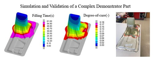
Compression resin transfer moulding (CRTM) has been widely used to manufacture automotive parts with reduced production cycle times. With the development of fast curing thermosetting resins, the CRTM process is a viable option for the high production rates in the transportation industry. However, the dynamic resin curing behaviour poses a potential risk of manufacturing defects in the part. In order to reduce the risk during the development of the tool and the process parameters, this paper proposes a modelling framework for the CRTM process when using fast curing resin systems. The work specifically focused on the coupling between heat transfer, resin cure, resin flow and preform compaction using a commercial code, PAM-RTM. The tool captures accurately the preform filling, temperature and resin pressure evolution during the injection and compression phase. The application of the framework was demonstrated for a complex 3D demonstrator. The predicted preform filling had an accuracy of 73% for the flow front evolution compared to the experimental results. This work demonstrates the validity of the framework proposed when dealing with resin systems that are challenging to process.

Graphical abstract

Keywords:

• Thermosetting resin
• process simulation
• resin flow
• compression resin transfer moulding

1. Introduction

Increase in demand for light weighting in transportation industry has resulted in the development of cost effective and energy efficient compression resin transfer moulding (CRTM) process. This process has been used to manufacture high performance fibre reinforced plastic (FRP) parts to replace the traditional aluminum and steel parts. These include automotive and other load-bearing components in the transportation sector. Due to rising market demand for accelerated production of these components, material suppliers have developed thermosetting resins that can cure at a faster rate. This resulted in a reduction in the cycle time demanded by the ground transportation industry [1].

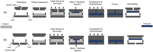
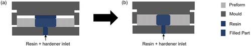
The CRTM process is described in Figure 1. The process involves injection of liquid resin through a dry preform placed inside a closed mould. During the resin injection phase, the top mould is kept partially open, to maintain an air gap. This gap facilitates the flow of the resin on top of the dry preform and subsequently through the preform during the compression phase. The difference between CRTM-1 and CRTM-2 in Figure 1 is based on the location of the injection gate.

Figure 1. Schematic description of the CRTM process showing the two options for the resin and hardener mixture injection location (a) in the top gap, (b) in the bottom of the preform.

The CRTM is a closed mould process. Therefore, it is extremely difficult to have in situ visualization of the process during experiments. The dynamic nature of the fast curing resins can also make the process difficult to understand experimentally. Hence, engineers have used process modelling to understand the dynamic nature of multiple physics inside a closed mould.

1.1. Previous work

Over the past three decades, most researchers have used process simulations to understand the behaviour of the CRTM process. Pham et al. [2] was one of the first researchers who successfully developed mould filling and compression simulation for the CRTM using finite element method for 2D geometries. Shojaei et al. [3] developed a finite element/control volume (FE/CV) based approach to simulate the CRTM process in three 3D with good agreement with the analytical solution. Nevertheless, these preliminary studies were limited to simple geometries and lacked experimental validation. Bhat et al. [4] and Simacek et al. [5] used Liquid Injection Moulding Simulation (LIMS) tool developed by University of Delaware to conduct an in-depth analysis of the CRTM process. The FE/CV based tool divided the process into three steps: injection into the gap, closure of the mould gap, and compression of preform. The injection step was simulated with 2D gap elements using lubrication theory. The validation experiments were conducted with short-shots on a B-pillar with reasonably good agreement. However, these works did not include the deformation of the preform before the onset of the preform compression.

In recent years, the effect of preform deformation during the injection stage of the CRTM process was investigated. Merotte et al. [6] assumed that the mould gap was entirely filled with resin during injection phase and the compression force of the mould was used as a pressure boundary condition on top of the preform to simulate the deformation of the preform during gap closure. Lee et al. [7,8] also developed a 1D transverse CRTM model to capture the hydrodynamic compaction effects during the process injection and compression phases. However, the works by [6,7] were confined to simple geometries and were not validated for complex 3D geometries. In a different approach, Marquette et al. [9] used a Fluid/Solid coupled solver, the latest feature of the PAM-RTM software from the ESI Group, to simulate the CRTM process. This approach helped determine the deformation of the preform during the injection-compression process by flexibility in data transfer between fluid and solid mechanics solvers. Another important feature of this approach was the use of an interpenetrating mesh to address the effect of the vanishing gap during the compression phase. To validate this simulation tool, Dereims et al. [10] conducted experiments on a truncated pyramid tool with a glass top mould. High-resolution cameras were used to capture the evolution of the flow front during injection and compression phases. The results showed good agreement between the simulation and the experiment. Although the authors simulated a complex geometry, the CRTM process was simplified by neglecting the heat transfer and resin cure reaction using isothermal conditions and non-reactive machine spindle oil as the resin.

Heat transfer and cure simulations have been well established for liquid composite moulding (LCM) processes [11–14]. In recent years, there has been an increase in the use of fast curing resins tailored to reduce process cycle times in aerospace and ground transportation industries [15,16]. However, the number of material models available on fast curing resins are limited [15,17,18]. Current research mostly focuses on either resin chemistry [19,20] or the mechanical properties of the composite parts once they are manufactured [21,22]. Moreover, with those types of resin, the curing reaction, and the development of the degree of cure take place during the injection step. Therefore, for the fast curing resins, the CRTM process must be modelled as a dynamic non-isothermal process. The earliest work on the non-isothermal RTM process was developed by Ruiz et al. [23] using a hybrid Finite Element/Finite Difference (FE/FD) methodology, which was extended to CRTM by Gupta et al. [24] for a 1D circular disc geometry. Experiments were conducted to determine the lower and upper bounds of processing parameters to develop an optimization scheme based on game theory. The optimization framework was restricted to simple 1D flow and was not tested on complex 3D structures. Keller et al. [25] developed a 2D multi-physics coupled model to simulate the CRTM process with different injection strategies: direct dosing, wet pressing, and gap injection using COMSOL Multiphysics. The simulation was able to capture the exotherms which were then validated by sensor readings from experiments with excellent agreement. The important aspect of this work was the inclusion of mould geometry in the simulation to investigate the effects of heat transfer between the mould and preform. Again, the simulations were restricted to simple 2D structures and were not tested on complex 3D parts.

1.2. Scope and overview

Based on the literature review available on the CRTM process, no single study has included all aspects of the process. The process is either solved as an isothermal problem or as a non-isothermal process with simple geometries. Furthermore, the available models do not include the post compression curing phase until the part is demoulded. Moreover, very few studies have considered the heat transfer between the mould and the preform [25,26]. Therefore, this work aims at addressing those gaps and modelling the entire manufacturing cycle, from the placement of the preform until the demoulding of the final part. Fully coupled heat transfer, resin flow, cure and compaction occurring during preheating, injection-compression and curing were simulated. Currently, only few numerical tools are available in the market which have the capability to simulate the CRTM process [5,9,10,27–29]. PAM-RTM was selected in this study because of its user-friendly graphical user interface (GUI) and its ability to implement custom cure kinetics and viscosity models of fast curing resins in the form of user subroutines using C scripts. The simulation findings were validated using 3D demonstrator parts with online temperature and pressure sensor recordings.

This paper is structured into five main sections. Section 2 outlines the numerical framework and governing equations employed in the simulation. Following that, Section 3 details both the experimental and simulation setups for a straightforward 3D flat plate geometry. Section 4 delves into the utilization of the data from Section 3 in the production of a complex 3D demonstrator component. Lastly, Section 5 offers the concluding remarks of the study.

2. Methodology

2.1. Numerical framework

The computational procedure for the entire CRTM process cycle is shown in Figure 2. The study employed a multistage computational approach to link preheating, resin injection/compression and curing simulations. The preheating simulation was initiated by initializing the material properties and the initial and boundary conditions. The resin injection/compression simulation was performed using the temperature distribution obtained from the previous preheating simulation. Similarly, the curing simulation was performed with the temperature and cure distribution results obtained from the injection/compression simulation. The link between the steps was done using extract/mapping feature available in PAM-RTM which maps the values of corresponding nodes to the next simulation step.

Figure 2. CRTM process simulation flow diagram showing the state variables [30].

The fluid solver solves the fluid flow and heat transfer equations. The initial values of the porosity, degree of cure, and temperature were fed to the fluid solver. Equation (3)(3) $$\nabla .\left(-\hspace{0.17em}\stackrel{̿}{\frac{K}{\mu }}.\nabla P\right)=0$$(3) is first solved using non-conforming finite element approximation. The Darcy velocity is then transferred to solve the LTE equation (Equation (5)(5) $${\rho }_c{C}_{\mathit{\text{pc}}}\frac{\partial T}{\partial t}+{\rho }_r{C}_{\mathit{\text{pr}}}\left(\overrightarrow{v}.\nabla T\right)=\nabla .\left(\stackrel{̿}{k}\nabla T\right)+\mathrm{Ø}{\rho }_r{H}_{\mathit{\text{tot}}}\frac{\partial \alpha }{\partial t}$$(5) ) using the Lesaint-Raviart formulation [23] to obtain the temperature and degree of cure output, which are transferred again to solve the momentum conservation equation (Equation (3)(3) $$\nabla .\left(-\hspace{0.17em}\stackrel{̿}{\frac{K}{\mu }}.\nabla P\right)=0$$(3) ). This procedure was followed for N time-steps to obtain the pressure field. The obtained pressure field was then transferred to the solid solver based on Equation (16)(16) $${\stackrel{̿}{\sigma }}_{\mathit{\text{overall}}}={\stackrel{̿}{\sigma }}_f+P\stackrel{̿}{I}$$(16) . The nonlinear solid mechanics problem was then solved by the solid solver (Equation (14)(14) $$\nabla .\stackrel{̿}{\mathrm{\hspace{0.17em}\sigma }}\left(\overrightarrow{u}\right)=\overrightarrow{f_B}$$(14) ) which results in deformation of the preform. The nodal displacement outcomes were subsequently used to update the porosity, which was then relayed back to the fluid solver. This iterative process persists until reaching the ultimate solution [31]. Figure 3 shows a flow chart of the working principle of the solver. The coupling frequency $f$ is the time at which the data transfer happens between the fluid and the solid solver. This value should be defined at the start of each simulation.

Figure 3. Numerical procedure to solve fluid-solid coupled problem [32].

2.2. Numerical treatment of the CRTM process

During the injection and compression of the mould, the resin impregnates the preform, which is governed by Darcy’s law: (1) $$\overrightarrow{v}=-\stackrel{̿}{\frac{K}{\mu }}.\nabla P$$(1) where $\overrightarrow{v}$ is Darcy’s velocity, $\stackrel{̿}{K}$ is the permeability of the reinforcement, $\mu$ is the viscosity of the resin and $\nabla P$ is the fluid pressure gradient. The resin was assumed to be incompressible when solving the CRTM problem. Based on the following assumption, the mass conservation equation was solved as follows: (2) $$\nabla .\overrightarrow{v}=0$$(2)

From Equation (1)(1) $$\overrightarrow{v}=-\stackrel{̿}{\frac{K}{\mu }}.\nabla P$$(1) and Equation (2)(2) $$\nabla .\overrightarrow{v}=0$$(2) , we get the following governing equation: (3) $$\nabla .\left(-\hspace{0.17em}\stackrel{̿}{\frac{K}{\mu }}.\nabla P\right)=0$$(3)

A fill factor associated with each element was used to track the flow front of the resin. The fill factor $F$ associated with each element was described using the following equation [33]: (4) $$F=\frac{V_r}{V_e.\mathrm{Ø}}$$(4) here $V_r$ and $V_e$ represents the volume of the resin and individual element respectively and $Ø$ is the porosity. The value of $F$ ranges from 0 to 1, indication the level of saturation in each element.

During the CRTM process, a significant amount of heat transfer takes place between the mould, resin, and fibres in the form of conduction, convection and exothermic chemical reactions caused by the fast curing resin. Therefore, the heat transfer problem can be problematic to solve. Local thermal equilibrium (LTE) model based on the first law of thermodynamics has been widely used to model LCM problems [34]. Here we used the same equation to solve for the heat transfer problem: (5) $${\rho }_c{C}_{\mathit{\text{pc}}}\frac{\partial T}{\partial t}+{\rho }_r{C}_{\mathit{\text{pr}}}\left(\overrightarrow{v}.\nabla T\right)=\nabla .\left(\stackrel{̿}{k}\nabla T\right)+\mathrm{Ø}{\rho }_r{H}_{\mathit{\text{tot}}}\frac{\partial \alpha }{\partial t}$$(5) where ${\rho }_c$ and ${\rho }_r$ represent the composite and resin density respectively, $C_{\mathit{\text{pc}}}$ and $C_{\mathit{\text{pr}}}$ are the heat capacity of composite and resin respectively, $T$ is the equilibrium temperature and $\stackrel{̿}{k}$ is the effective thermal conductivity tensor. $H_{\mathit{\text{tot}}}$ is the total heat of reaction and $\alpha$ is the degree of cure of the resin. The last term on the right-hand side of the equation takes into account the effect of the reaction kinetics of the resin. This equation was used for solving preheating, mould filling and curing problems. The average material property was calculated using the following equations. Here r and f represent resin and fibre respectively: (6) $${\rho }_c{C}_{\mathit{\text{pc}}}=\mathrm{Ø}{\rho }_r{C}_{\mathit{\text{pr}}}+(1-\mathrm{Ø}){\rho }_f{C}_{\mathit{\text{pf}}}$$(6) (7) $$\frac{1}{k}=\frac{\mathrm{Ø}}{k_r}+\frac{\left(1-\mathrm{Ø}\right)}{k_f}$$(7)

The reaction rate $R_{\alpha }=\frac{\partial \alpha }{\partial t}$ of the fast curing reaction during the CRTM process was modelled using an Arrhenius type equation developed by Ruiz et al. [35]: (8) $$R_{\alpha }={(K_1+K}_2{\alpha }^m\left){(1-\alpha )}^{n}f\right(\alpha )$$(8) (9) $$K_i=A_i\mathrm{\text{exp}}\hspace{0.17em}\left(\frac{-E_{\mathit{\text{ai}}}}{\mathit{\text{RT}}}\right)$$(9) (10) $$f\left(a\right)=\frac{1}{1+\mathrm{\text{exp}}\left[C\right(\alpha -\left({\alpha }_{C0}+{\alpha }_{\mathit{\text{CT}}}T\right)\left)\right]}$$(10) where $E_{\mathit{\text{ai}}}$ is the activation energy, $R$ is the universal gas constant, and $A_i$ is the preexponential factor. $f\left(a\right)$ is used to account for the low-speed reaction to diffusion. $A_i,m,n,C,{\alpha }_{C0}\mathit{\text{ and }}{\alpha }_{\mathit{\text{CT}}}$ are the fitting parameters.

Conservation of mass for the highly reactive chemical species is governed by the advection equation which is expressed as: (11) $$\frac{\partial \alpha }{\partial t}+\overrightarrow{v}.\nabla \alpha =R_{\alpha }$$(11)

The initial value of the $\alpha$ was set at 0.01 to solve Equation (11)(11) $$\frac{\partial \alpha }{\partial t}+\overrightarrow{v}.\nabla \alpha =R_{\alpha }$$(11) . The second term of the Equation (11)(11) $$\frac{\partial \alpha }{\partial t}+\overrightarrow{v}.\nabla \alpha =R_{\alpha }$$(11) governs the velocity of the resin and source term on the right-hand side of the equation measures the cure rate.

The temperature and cure dependent viscosity $\mu$ was described using the model developed by Castro and Macosko [36]: (12) $$\mu =A_{\mu }\mathrm{e}\mathrm{\text{xp}}\left(\frac{E_{\mu }}{\mathit{\text{RT}}}\right){\left(\frac{{\alpha }_g}{{\alpha }_g-\alpha }\right)}^{a+b\alpha }$$(12) where $R$ is the universal gas constant, ${\alpha }_g$ is the degree of cure at gelation, $A_{\mu }$ is the exponential factor, $E_{\mu }$ is the activation energy, and a and b are the exponents. The values were determined experimentally using a rheometer.

A heat transfer coefficient (HTC) was defined between the mould and the preform. It was assumed that the contact between the preform and the mould is never a perfect one. Figure 4 shows the representation of the contact between the preform and mould to define the HTC. The equation used to calculate HTC was given as follows [30]: (13) $$\mathit{\text{HTC}}=\frac{k_a}{e}$$(13) where $k_a$ is the thermal conductivity of the air, $e$ is the interface thickness, $T_1$ and $T_2$ are the mould and preform temperature respectively.

Figure 4. Heat transfer preform-mould interface showing the temperature variation assumption across the interface [30].

The fibre reinforcement was assumed to be a deformable medium. The large stresses and strains experienced by the reinforcement during the injection and compression sequence cause a significant change in porosity. This behaviour was captured using momentum conservation equation for solid phase as [10]: (14) $$\nabla .\stackrel{̿}{\mathrm{\hspace{0.17em}\sigma }}\left(\overrightarrow{u}\right)=\overrightarrow{f_B}$$(14) where $\stackrel{̿}{\sigma }$ is the Cauchy’s stress tensor, $\overrightarrow{u}$ is the displacement vector and $\overrightarrow{f_B}$ is the body force vector. Traditionally, the applied stress was related to the change in porosity using semi-empirical relations [32]. However, here we use the method developed by Celle et al. [13], where the porous domain was represented as an orthotropic homogenous medium composed of incompressible fibres. The following Lagrangian formulation was used [37]: (15) $$J\left(\overrightarrow{x},t+\Delta t\right)\left(1-\mathrm{Ø}\left(\overrightarrow{x},t+\Delta t\right)\right)=J(\overrightarrow{x},t)(1-\mathrm{Ø}(\overrightarrow{x},t\left)\right)$$(15) where $\overrightarrow{x}$ is the position vector, $Ø$ is the porosity of the fibre reinforcement and $J$ is the Jacobian of the transformation.

The fibre compaction pressure was coupled with the resin pressure using Terzaghi’s relationship [38]: (16) $${\stackrel{̿}{\sigma }}_{\mathit{\text{overall}}}={\stackrel{̿}{\sigma }}_f+P\stackrel{̿}{I}$$(16) where ${\stackrel{̿}{\sigma }}_{\mathit{\text{overall}}}$ is the overall stress exerted. ${\stackrel{̿}{\sigma }}_f$ is the stress generated on the fibre, $P$ is the hydrostatic resin pressure and $\stackrel{̿}{I}$ is the unit tensor. Based on the pressure field calculated using Equation 10(10) $$f\left(a\right)=\frac{1}{1+\mathrm{\text{exp}}\left[C\right(\alpha -\left({\alpha }_{C0}+{\alpha }_{\mathit{\text{CT}}}T\right)\left)\right]}$$(10) , the above equation calculates the amount of stress encountered by the fibres. This value was then used to calculate the nonlinear finite strains that cause variations in porosity. The porosity change was then linked to permeability. Permeability can be calculated using power law: (17) $$K=p{\left(1-\mathrm{Ø}\right)}^q$$(17) where p and q are fitting parameters.

2.3. Material model input

Multiple material models are to be defined to run a non-isothermal 3D CRTM simulation. The fast curing resin cure kinetic and viscosity model developed by Barcenas et al. [15] were implemented as a user subroutine in the form of C scripts. A summary of the material and process parameters are shown in Table 1.

Table 1. Material and process parameters used in the simulations.

Cure kinetics [15]
$A_1=-53090 s^{-1}$	Pre-exponential factor 1
$E_1=52160 J/\mathit{\text{mol}}$	Activation energy 1
$A_2=12280 s^{-1}$	Pre-exponential factor 2
$E_2=43750 J/\mathit{\text{mol}}$	Activation energy 2
$H_T=440 J/g$	Total heat of reaction
$m,n=0.10,1.69$	Exponents
$C,{\alpha }_{\mathit{\text{co}}}=200,0.911$	Diffusion parameters
Rheology [15]
$A_{\mu }=1.68*{10}^{-6} \mathit{\text{Pa}}.s$	Pre-exponential factor
$E_{\mu }=31780 J/\mathit{\text{mol}}$	Activation energy
${\alpha }_g=0.78$	Degree of cure at gel point
$a,b=0.8,4.50$	Exponents
Heat transfer properties [25]
${\rho }_r,{\rho }_f,{\rho }_m=1180,2600,7800 \mathit{\text{kg}}/m^3$	Density
$C_{\mathit{\text{pr}}},C_{\mathit{\text{pf}}},C_{\mathit{\text{pm}}}=1500,800,515 J/(\mathit{\text{kg}}.K)$	Specific heat
$k_r,k_f,k_m=0.2,1.2,50 W/(m.K)$	Thermal conductivity
Process parameters
$V_{f01}=0.402$	Initial preform volume fraction
$V_{f02}=0.482$	Initial pinch volume fraction
$U=1 \mathit{\text{mm}}/s$	Mould closing speed
$T_{\mathit{\text{inj}}}=20°C$	Resin injection temperature
$T_{\mathit{\text{um}}},T_{\mathit{\text{lm}}}=100,95°C$	Upper and lower mould temperatures
$T_{\mathit{\text{amb}}}=22°C$	Ambient room temperature
$P_{\mathit{\text{inj}}},P_{\mathit{\text{vent}}}=550,-100 \mathit{\text{kPa}}$	Resin injection and vent pressure
$\mathit{\text{HTC}}=480 W/(m^2.K)$	Heat transfer coefficient
$e=2*{10}^{-4} m$	Interface thickness

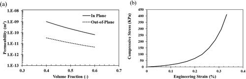
The non crimp glass fibre (NCF) material models include permeability and compression data. The in-plane and out-of-plane permeabilities of the NCF glass fibre were measured using the in-house laboratory equipment. The permeability was calculated for volume fractions ranging between 0.4 − 0.6 with techniques used in [39,40] and permeability was implemented as a function of volume fraction in the form of a table graph as shown in Figure 5a. The preform compaction was measured using an MTS Insight 5 kN universal testing machine. Dry fibres with a layup sequence of [(0/90)]_4S, which was similar to the layup sequence to the manufactured parts were tested using the procedure outlined in the latest benchmarking exercise [41]. Figure 5b shows the compaction response of TG15N glass fibre. This was also implemented in the form of a table graph.

Figure 5. (a) In-plane and out-of-plane permeability and (b) fibre bed compaction response of TG15N NCF.

3. Model validation

3.1. Experimental setup and materials

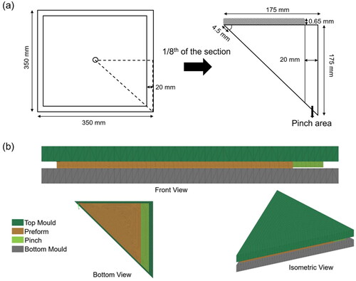
In this work, the initial focus was on examining a simple flat plaque geometry to understand the CRTM process in detail. The experimental set up consisted of a P20 steel plaque tool, as shown in Figure 6a. The flat plate tool was housed in a 1.25 kilo tons compression press from PEI (Pinette Emidecau Industries). The tool was designed at the National Research Council Canada (NRC) to make parts with dimensions of 350 mm x 350 mm and a thickness range of 1-10 mm. A pinch area, reducing the thickness by 0.65 mm all around the preform perimeter was designed to help keep the fibre reinforcement in place when the resin was injected. The resin injection gate was located at the centre of the bottom mould.

Figure 6. (a) CRTM mould setup for flat part, (b) TG15N NCF glass fibre preform, (c) location of sensors on the bottom mould, and (d) the schematic showing the location of the sensors.

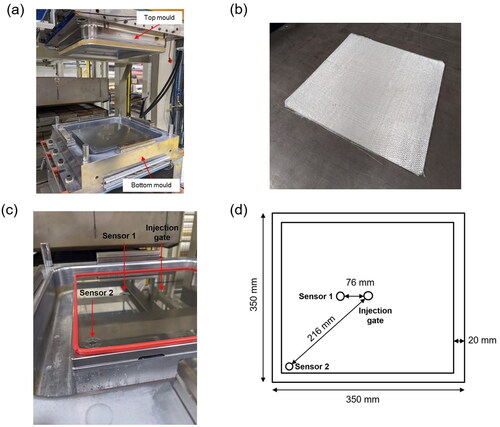
Prime 130 fast curing epoxy resin from Gurit was used to perform experiments. The resin system used here was a one-part epoxy and one-part hardener mixed in the ratio 100:25 by weight. The fibre reinforcement used for this work was an NCF from Texonic Inc. The fibre has an areal density of 518 g/m² and each layer of fabric had an approximate thickness of 0.45 mm. The preform was prepared using a layup sequence [(0/90)]_4S. An Epikote 06720 epoxy thermoplastic binder was applied in between each ply of the preform. The preform was then vacuum bagged and placed in an oven at 100 °C for 15 min to be stabilized.

The mould was preheated to the desired temperature. The preform was placed on a preheated mould and the top mould was then moved down until there was a gap of 1 mm between the two cavity surface. A known amount of resin and hardener mixture was injected through the injection gate located at the centre of the bottom mould. As soon as the injection was stopped, the top mould was moved downward to compress the preform and achieve full impregnation.

To visualize the flow front inside the tool cavity, interrupted filling tests (short shots) were performed. Due to the inherently fast curing nature of the resin, the flow front ceases within a minute of discontinuing the resin injection due to the sharp increase in resin viscosity. Consequently, a clearly defined flow front was obtained, which was used to validate the simulation results. The test matrix used for interrupted filling tests is presented in Table 2.

Table 2. Interrupted filling test matrix with corresponding time.

Test No.	Time (sec)
1	5
2	30
3	60 (End of injection)
4	61.23 (End of compression)

To further validate the simulation results, two GEFRAN WE26-M-P03M pressure transducers with a built-in thermocouple were placed in a strategic location within the tool bottom surface as shown in Figure 6c,d. The first sensor was located close to the injection gate, whereas the second sensor was located closer to the vent diagonally from the injection gate. The experiments were conducted, and the data were captured immediately from the placement of the preform up until the demoulding of the fully cured part.

3.2. Simulation setup

3.2.1. Geometry definition

The detailed dimensions of the geometry are shown in Figure 7a. Given the resin injection gate’s central placement on the bottom mould, symmetry allowed us to simulate only one-eighth of the section. This study incorporates several simplification strategies. While the transition between the tool pinch and the central main surface is in the form of an inclined surface, the model was simplified by assuming a step transition from the central to the pinch area with a flat mould pressing on an already deformed reinforcement. A 3D geometry was constructed using the features available in PAM-RTM as shown in Figure 7b. The top mould was 10 mm thick to include the heat transfer effects from the mould and was made wider than the preform to accommodate the possible deformations during the compression sequence. The preform was divided into two regions: (i) the central preform region (orange) and (ii) the pinch region (light green).

Figure 7. (a) Schematic of the simulation geometry representing 1/8^th of the preform, and (b) meshed geometry of 1/8^th section showing the modelling of the mould pinch area.

In the bottom injection CRTM process, the modelling approach slightly differs from the traditional top injection method. Here the resin directly comes in contact with the preform already positioned in the mould. Despite operating at lower pressures compared to the traditional RTM process [42,43], these pressures are still sufficient to induce movement of the preform in the transverse direction. To streamline the modelling process, it was assumed that the preform occupied the entire mould cavity during resin injection. Consequently, the preform geometry possesses greater thickness and is characterized by a lower equivalent fibre volume fraction. Figure 8 provides a schematic illustration of the assumptions made in this study. Furthermore, it is assumed that the contact between the mould and the preform is not perfect and a heat transfer coefficient is imposed between them as explained in section 2.2. The mould, preform and pinch sections were modeled using 160,357 tetrahedral 3D elements. The simulation was performed on an Intel^® Core^™ i-7 4770 CPU with four cores.

Figure 8. Schematic showing the assumption made during the modelling of the CRTM process, (a) injection of resin and hardener with the inclusion of the gap and, (b) injecting considering preform decompression by adjusting the preform fibre volume fraction eliminating the gap.

3.2.2. Model assumption

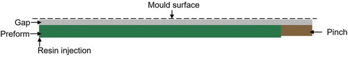
In this work, due to experimental tooling configurations, CRTM process where the resin was injected directly into the preform (as shown in Figure 1b) was used. As the resin is injected into the preform, the decompression effect [44] can cause thickening of the preform, as shown in Figure 8. To streamline the process simulation, it was assumed that the preform occupied the entire cavity inside the mould during resin injection. Therefore, intitial thickness of the preform was considered as 4 mm (fully occupying the cavity) instead of 3.35 mm (actual preform thickness). To check for the effect of decompression, a model was defined in PAM-RTM to include the gap with zero porosity. The front-view of the model is described in Figure 9.

Figure 9. Front view of the geometry of 1/8th section of the model with the inclusion of the gap to check for preform decompression.

3.3. Results and discussion

3.3.1. Preform decompression

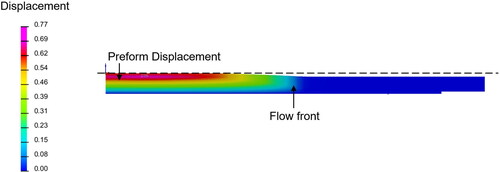
The initial step in the simulation process involved confirming the validity of the assumption described in Figure 8b. As shown in Figure 10, the flow simulation demonstrated the progressive decompression of the preform as the resin flow front progresses [45], filling the predefined gap between the preform and the tool upper surface. Unfortunately, the simulation did not reach full convergence due to the intrusion of gap elements into the preform as more resin was injected [9]. Therefore, we could confidently proceed further with the assumption made in Figure 8 that the simulations could be carried out with the preform completely occupying the mould cavity.

Figure 10. The results showing the effect of decompression of the preform (displacement in mm) with the progression of the flow front.

3.3.2. Interrupted flow analysis

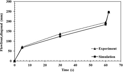
The interrupted filling test matrix outlined in Table 2 was executed and the corresponding simulation results were compared. Initially, resin was injected into the mould for a duration of 5 s before being stopped. The resulting flow front pattern obtained was compared with the simulation results. This comparison encompassed both the flow front’s distance along the x-direction and the diagonal of the x-y plane. At this point, the flow front had traversed a distance of 71 mm from the injection gate. The simulation predicted a distance of 67 mm with 95% accuracy. For 30 s injection, the simulation predicted the flow front with 91% accuracy. At 60 s, the flow front had reached the end of the x-direction, and the diagonal distance was compared. The simulation exhibited strong concordance with the experimental data with 94% accuracy. The visual representation of the experiment-simulation with fill factor comparison is shown in Figure 11 a–c. The flow front prediction was in good agreement with the experimental results. Additionally, the simulation also captures the deviation of flow front direction from the preform to the pinch section, as shown in Figure 11d. To effectively gauge the resemblance between the experimental and simulation outcomes, the diagonal flow front distance was graphed against time, as shown in Figure 12, highlighting the close agreement between them (greater than 90%). The difference can be attributed to the use binder powder in the preforming process. The activation at processing temperature (100 ⁰C), causes dissolution of the binder powder into the fibre tows resulting shrinkage of the fibre [46]. This results in an increase in permeability. Furthermore, Tonejc et al. [47] have shown the increase of permeability in the in-plane direction by approximately 20% at processing temperatures while using epoxy resin with powdered binder. Moreover, binders can have an effect on the viscosity of the fast curing resin which is an area yet to be explored.

Figure 11. Progression of flow front at different time intervals: experiment vs simulated flow patterns with fill factor at (a) 5 s, (b) 30 s, (c) 60 s (end of injection) and (d) simulation predicting the deviation observed at the transition of preform and the pinch section at the end of injection (60 s).

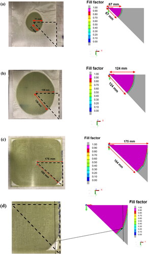
Figure 12. Flow front diagonal distance comparison between experiment and simulation.

3.3.3. Sensor analysis

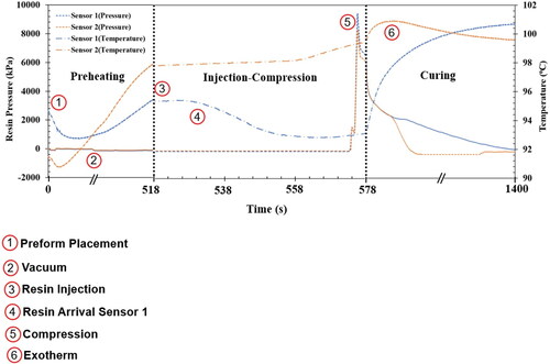
The sensor data for the entire process, from preform placement until the demoulding step, is illustrated in Figure 12. Initially, the preform was placed on a preheated mould. This resulted in a slight decrease in the temperature reading on both sensors by approximately 2 ⁰C, as the preform was cooler than the mould, as evident at point 1 in Figure 13. In terms of pressure, point 2 in Figure 13 showed a slight decrease from 0 to −100 kPa as the vacuum was turned on. Once the preform attained the mould temperature, the resin with an initial temperature of 20 ⁰C (room temperature) was injected through the injection gate at point 3. When the resin flow front reached sensor 1, a noticeable drop in temperature was observed at point 4. Once the targeted amount of resin was injected into the tool cavity, the compression sequence was activated, resulting in a substantial spike of approximately 9000 kPa in the resin pressure, as indicated at point 5. Subsequently, the curing phase was then initiated and the preform was maintained in the compressed state for approximately 10 min. The rise in temperature, as seen by sensors 1 and 2, illustrated in region 6, was attributed to the exothermic reaction of the resin.

Figure 13. Pressure and temperature data recording of the two sensors for the entire CRTM process: preheating, injection compression and curing. The x-axis has been segmented to show the scale only for injection-compression phase.

The measured temperature and pressure histories were validated using the virtual sensor functionality available in PAM-RTM. These virtual sensors were positioned in the exact locations as the actual sensors, as shown in Figure 14. The simulation showed that the preform quickly attained the temperature of the mould, a greater emphasis was given to the injection-compression and post compression cure regions. Initially, the temperature history at the injection-compression region was examined. The measured temperature data was compared with the virtual sensor simulation data and was plotted against time, as illustrated in Figure 15a. The simulation successfully captured the temperature decrease at the sensor 1 as the colder resin passed through it. The temperature at the sensor two remained constant since the resin had already reached the temperature of the mould and the preform, which was again captured by the simulation.

Figure 14. (a) Schematic showing the location of the two sensors on the 1/8^th section of the part. (b) Placement of virtual sensors at the same location on the model geometry in PAM-RTM.

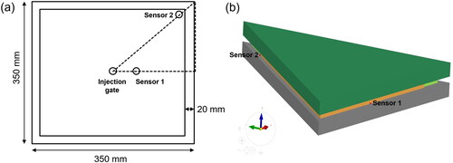
Figure 15. (a) Comparison between the simulation and experimental data of temperature for both sensors during the (a) injection-compression and (b) curing phase. (c) Comparison between simulation and experimental data of pressure during injection-compression phase.

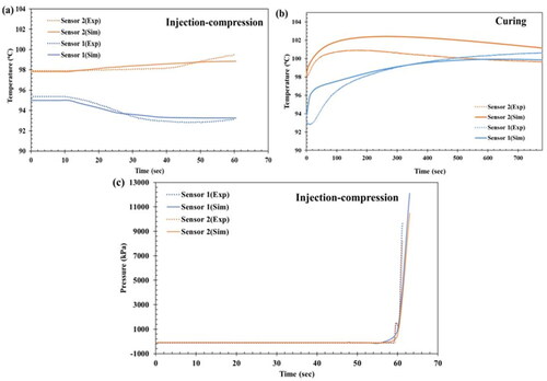
Next step involved analyzing the curing phase of the CRTM process. The nodal temperatures at the end of the injection-compression phase were set as the initial temperature condition for the curing section. The simulation results captured the sudden rise in resin temperature due to exothermic reaction, as shown in Figure 15b.

Finally, Figure 15c presents the pressure comparison between the experimental and simulation results. Even though there is a difference of approximately 1400 kPa, the difference in pressure between the two sensors for experiment and simulation was consistent. This difference can be attributed to the deviation of experimental values from the material models used in the simulation.

4. Model application

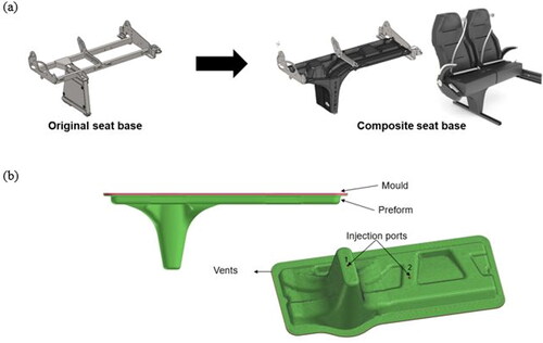
The modelling approach used in the previous sections was applied to simulate the CRTM process to manufacture a one-piece integrated composite seat base structure for a long-distance coach. Figure 16a illustrates the current welded steel design and the corresponding composite design. The same preform and resin system used for the flat plaque experiment were used to manufacture this complex structure. Because of the geometry complexity, sensors were not machined into the mould. Therefore, only interrupted filling tests were conducted to validate the simulation results.

Figure 16. (a) Welded steel assembly and the corresponding composite design, and (b) meshed mould and preform geometry with injection gate and vent locations.

4.1. Model setup

A 3D CAD model of the seat base design was imported into the PAM-RTM. Using the geometry features available, a 3D top mould and preform were constructed, as shown in Figure 16b. The bottom mould was excluded to reduce the computation time. The mould and preform were meshed using 1081518 3D tetrahedral elements. Two injection gate locations were chosen strategically to reduce the total cycle time, and vacuum was applied to the perimeter of the part, as shown in Figure 17. The material models described in Table 2 were implemented with the process parameters listed in Table 3.

Figure 17. Simulation showing resin injected simultaneously using two ports and the corresponding final part produced based on the simulation.

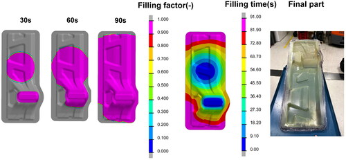
Table 3. Material and process parameters used for the demonstrator simulations.

Process Parameters
$V_{\mathit{f}01}=0.37$	Initial preform volume fraction
$U=1 \mathit{\text{mm}}/s$	Mould closing speed
$T_{\mathit{\text{inj}}}=25°C$	Resin injection temperature
$T_{\mathit{\text{um}}},T_{\mathit{\text{lm}}}=70,70°C$	Upper and lower mould temperatures
$T_{\mathit{\text{amb}}}=22°C$	Ambient room temperature
$P_{\mathit{\text{inj}}},P_{\mathit{\text{vent}}}=90,-14 \mathit{\text{psi}}$	Resin injection and vent pressure

4.2. Results and discussion

4.2.1. Simulation and experiment with one injection port

The simulation took a total time of approximately 12 h on an Intel^® Core^™ i-7 4770 CPU with four cores. The first simulation was performed by injecting only by one injection port at the foot of the seat base. The initial volume fraction was calculated assuming the preformed filled the entire mould cavity with a gap of 2 mm as discussed in section 3.2. The simulation results for filling time, degree of cure and viscosity are shown in Figure 18.

Figure 18. Filling time, degree of cure and viscosity development for single port injection at the end of compression sequence (281 s).

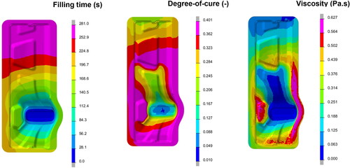
The simulation results showed a total filling time of 280 s. The experiment conducted in the same conditions resulted in a total filling time of 205 s. A difference of 75 s was considered close enough for a complex part with large dimensions (greater than 1 m). The visualization of the predicted resin degree of cure and viscosity was important to identify the extent of cure of the resin at the end of resin injection-compression phase and if the resin was close to gelation. For example, in Figure 18, the maximum degree of cure of the resin at the end of compression was 0.401 which was well below the degree of cure at gel point (0.78) for the resin used in this study. Therefore, we can be confident to inject the resin with the process parameters chosen for that simulation.

4.2.2. Interrupted filling test

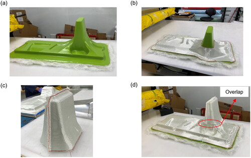
The validation of the seat base simulation was done using interrupted filling test. The resin was injected at port one for 60 s, followed by the compression sequence. Similarly, simulations were performed for the same conditions as the experiments, and the results are shown in Figure 19. The final flow front, after the compression stage extended beyond the second injection port, while the simulation results slightly lagged. One of primary reasons for this discrepancy is the difference between the modelled preform and the experimental preform. The complex part design led to a complex preform with local changes in terms of fabric shearing and fibre volume fraction that are not captured by the simulation. As shown in Figure 20a–d, the preforming of seat base was a complex process which involved two separate sections. The preform for the foot and rest of the part was draped separately on the 3d printed seat base plug. In Figure 20d, the overlapping at the joining region caused an increase local volume fraction leading to the dry spot formation as shown in Figure 19.

Figure 19. Short shot test for comparing the experimental and simulation results for the demonstrator at an injection time of 60 s followed by compression.

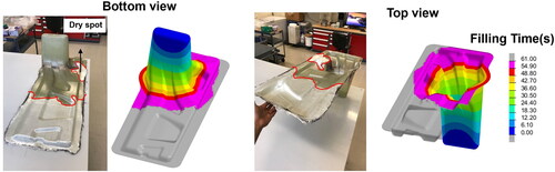
Figure 20. (a) 3d Printed seat base plug on which the preform will be draped, (b) first part of the preform draped on the seat base plug, (c) second part (foot) of the seat base preform, and (d) completed draping of preform on the plug with an overlapped section.

4.2.3. Simulation and experiment with two injection ports

The second part of the simulation consisted of injecting the resin using two injection ports to reduce the cycle time. In this case, the simulation results predicted a reduction of the injection time by 190 s and no dry spots or porosity was seen. One of the major manufacturing concerns was the possible formation of voids when the two flow fronts meet. The results of the experiment validated the simulation as a 2-injection gate part with good impregnation was obtained. The different stages of the flow front evolution for multiple port injection are shown in Figure 17 along with the manufactured part.

5. Conclusions

In this study, the 3D CRTM process was simulated using a fluid/solid coupled approach to take into account all the thermal and physical phenomena occurring during the entire process cycle (heat transfer, resin flow, resin cure, and fibre compaction). In particular, numerical models included the mould and accounted for the heat transfer between mould, the preform and the injected resin. Interrupted filling tests were successfully used to compare experimental and simulation results at different injection times for a 3D flat plaque geometry and the numerical approach was validated.The simulation accurately predicted the flow front’s progression with an accuracy of greater than 80%. Furthermore, the simulations successfully captured the deviation of the flow front with local change in preform compaction and permeability.

Experimental data from in-mould sensors used to monitor the entire process, from the placement of the preform to demoulding, highlighted important changes in pressure and temperature. The virtual sensors used in PAM-RTM further validated the measured values, showing excellent agreement with the actual data. The sensors also played a pivotal role in capturing the exothermic reactions of the fast curing resin, providing crucial insights into its curing state compared to simulated model.

Finally, this simulation approach was extended to model the CRTM manufacturing of a large complex composite seat base structure. Despite the intricate nature of the geometry, the interrupted filling tests validated the simulation results. Total fill time for the complete injection of the part showed an accuracy of 73% with good impregnation and minimal dry spots.

Overall, this work demonstrated the effectiveness of the simulation approach to replicate the entire manufacturing cycle from the placement of the preform till demoulding to create a large scale complex ground transportation part using fast curing resin. For complex geometries, the validation experiments showed the need to include the preform shearing data to increase the accuracy of the simulation. Furthermore, the inclusion of the influence of binder on permeability and the effect of the binder on the resin viscosity warrants a further study to streamline the material models. The insights gained from this work can be utilized to further optimize the CRTM process to help the ground transportation industry.

Authors’ contributions

Sidharth Sarojini Narayana: Conceptualization, Data curation, Software, Formal analysis, Methodology, Visualization, Writing – original draft. Loleï Khoun: Project administration, Funding acquisition, Writing – review & editing. Paul Trudeau: Project administration, Writing – review & editing. Nicolas Milliken: Project Administration, Writing – review and editing. Pascal Hubert: Supervision, Writing – review & editing.

Acknowledgments

The Authors would like to thank Natural Sciences and Engineering Research Council of Canada (NSERC) for funding the work. The authors would also like to thank our project partners Prevost, AOC resins, Gurit. Teijin, Norplex-Micarta, NanoXplore, Novation Tech, Effman, Texonic and RAMPF composites for their support. The authors would like to thank Dr. Arnaud Dereims from ESI group for technical support on PAM-RTM.

Disclosure statement

No potential conflict of interest was reported by the author(s).

References

- Khoun L, Trudeau P. SNAP RTM: a cost-effective compression-RTM variant to manufacture composite component for transportation applications. Novi, Michigan, USA: Society of Plastics Engineers; 2018.
- Pham X-T, Trochu F, Gauvin R. Simulation of compression resin transfer molding with displacement control. J Reinf Plast Compos. 1998;17(17):1525–1556. doi: 10.1177/073168449801701704.
- Shojaei A. Numerical simulation of three-dimensional flow and analysis of filling process in compression resin transfer moulding. Compos Part Appl Sci Manuf. 2006;37(9):1434–1450. doi: 10.1016/j.compositesa.2005.06.021.
- Bhat P, Merotte J, Simacek P, et al. Process analysis of compression resin transfer molding. Compos Part Appl Sci Manuf. 2009;40(4):431–441. doi: 10.1016/j.compositesa.2009.01.006.
- Simacek P, Advani SG, Iobst SA. Modeling flow in compression resin transfer molding for manufacturing of complex lightweight high-performance automotive parts. J Compos Mater. 2008;42(23):2523–2545. doi: 10.1177/0021998308096320.
- Merotte J, Simacek P, Advani SG. Resin flow analysis with fiber preform deformation in through thickness direction during compression resin transfer molding. Compos Part Appl Sci Manuf. 2010;41(7):881–887. doi: 10.1016/j.compositesa.2010.03.001.
- Lee J, Duhovic M, Allen T, et al. Computational modelling and analysis of transverse liquid composite moulding processes. Compos Part Appl Sci Manuf. 2023;167:107433. doi: 10.1016/j.compositesa.2023.107433.
- Lee J, Duhovic M, Allen T, et al. Sensitivity of transverse Liquid Composite Moulding processing predictions to variations in constitutive data. Adv Manuf Polym Compos Sci. 2023;9(2266288). doi: 10.1080/20550340.2023.2266288.
- Marquette P, Dereims A, Ogawa T, et al. Numerical methods for 3D compressive RTM simulations. Munich, Germany; 2017.
- Dereims A, Zhao S, Yu H, et al. 2017 Compression resin transfer molding (C-RTM) simulation using a coupled fluid-solid approach. DEStech Publications, Inc. doi: 10.12783/asc2017/15224.
- Gao DM, Trochu F, Gauvin R. Heat transfer analysis of non-isothermal resin transfer molding by the finite element method. Mater Manuf Process. 1995;10(1):57–64. doi: 10.1080/10426919508934998.
- Ruiz E, Achim V, Trochu F. Coupled non-conforming finite element and finite difference approximation based on laminate extrapolation to simulate liquid composite molding processes. Part i: isothermal flow. Sci Eng Compos Mater. 2007;14(2):85–112. doi: 10.1515/SECM.2007.14.2.85.
- Celle P, Drapier S, Bergheau J-M. Numerical modelling of liquid infusion into fibrous media undergoing compaction. Eur J Mech - ASolids. 2008;27(4):647–661. doi: 10.1016/j.euromechsol.2007.11.002.
- Abisset-Chavanne E, Chinesta F. Toward an optimisation of the reactive resin transfer molding process: thermo-chemico-mechanical coupled simulations. Int J Mater Form. 2014;7(2):249–258. doi: 10.1007/s12289-013-1124-0.
- Barcenas L, Narayana SS, Khoun L, et al. Thermochemical and rheological characterization of highly reactive thermoset resins for liquid moulding. J Compos Mater. 2023;57(19):3013–3024. doi: 10.1177/00219983231181640.
- Zhao X, Huang Z, Song P, et al. Curing kinetics and mechanical properties of fast curing epoxy resins with isophorone diamine and N ‐(3‐aminopropyl)‐imidazole. J of Applied Polymer Sci. 2019;136(37):47950. doi: 10.1002/app.47950.
- Bernath A, Kärger L, Henning F. Accurate cure modeling for isothermal processing of fast curing epoxy resins. Polymers (Basel). 2016;8(11):390. doi: 10.3390/polym8110390.
- Baran I, Akkerman R, Hattel JH. Material characterization of a polyester resin system for the pultrusion process. Compos Part B Eng. 2014;64:194–201. doi: 10.1016/j.compositesb.2014.04.030.
- Pradhan S. Synthesis and advances in rapid curing resins. In Rapid Cure Compos. Elsevier; 2023. p. 15–31. doi: 10.1016/B978-0-323-98337-2.00004-3.
- Capricho JC, Fox B, Hameed N. Multifunctionality in Epoxy Resins. Polym Rev. 2020;60(1):1–41. doi: 10.1080/15583724.2019.1650063.
- Groh F, Kappel E, Hühne C, et al. Investigation of fast curing epoxy resins regarding process induced distortions of fibre reinforced composites. Compos Struct. 2019;207:923–934. doi: 10.1016/j.compstruct.2018.09.003.
- Keller A, Chong HM, Taylor AC, et al. Core-shell rubber nanoparticle reinforcement and processing of high toughness fast-curing epoxy composites. Compos Sci Technol. 2017;147:78–88. doi: 10.1016/j.compscitech.2017.05.002.
- Ruiz E, Trochu F. Coupled non-conforming finite element and finite difference approximation based on laminate extrapolation to simulate liquid composite molding processes. Part II: non-isothermal filling and curing. Sci Eng Compos Mater. 2007;14(2):113–144. doi: 10.1515/SECM.2007.14.2.113.
- Gupta A, Kelly PA, Ehrgott M, et al. A surrogate model based evolutionary game-theoretic approach for optimizing non-isothermal compression RTM processes. Compos Sci Technol. 2013;84:92–100. doi: 10.1016/j.compscitech.2013.05.012.
- Keller A, Dransfeld C, Masania K. Flow and heat transfer during compression resin transfer moulding of highly reactive epoxies. Compos Part B Eng. 2018;153:167–175. doi: 10.1016/j.compositesb.2018.07.041.
- Sobotka V, Delaunay D. Analysis and control of heat transfer in an industrial composite mold in RTM polyester automotive process. J Reinf Plast Compos. 2007;26(9):881–901. doi: 10.1177/0731684407076731.
- Seuffert J, Kärger L, Henning F. Simulating mold filling in compression resin transfer molding (CRTM) using a three-dimensional finite-volume formulation. J Compos Sci. 2018;2(2):23. doi: 10.3390/jcs2020023.
- Seuffert J, Rosenberg P, Kärger L, et al. Experimental and numerical investigations of pressure-controlled resin transfer molding (PC-RTM). Adv Manuf Polym Compos Sci. 2020;6(3):154–163. doi: 10.1080/20550340.2020.1805689.
- Simacek P, Niknafs Kermani N, Advani SG. Coupled process modeling of flow and transport phenomena in LCM processing. Integr Mater Manuf Innov. 2022;11(3):363–381. doi: 10.1007/s40192-022-00268-1.
- PAM-RTM. 2020. 5 User’s Guide 16.0. ESI Group 2020. Available from: www.esi-group.com
- Dereims A, Chatel S, Marquette P, et al. Accurate liquid resin infusion simulation throug a Fluid-Solid coupled approach. 2017.
- Gutowski TG, Morigaki T, Cai Z. The consolidation of laminate composites. J Compos Mater, 1987;21(2):172–188. doi: 10.1177/002199838702100207.
- Trochu F, Gauvin R, Gao D-M. Numerical analysis of the resin transfer molding process by the finite element method. Adv Polym Technol. 1993;12(4):329–342. doi: 10.1002/adv.1993.060120401.
- Sherratt A, Straatman AG, DeGroot CT, et al. Investigation of a non-equilibrium energy model for resin transfer molding simulations. J Compos Sci. 2022;6(6):180. doi: 10.3390/jcs6060180.
- Ruiz E, Waffo F, Owens J, et al. Modeling of resin cure kinetics for modling cycle optimization. Douai, France; 2006.
- Castro JM, Macosko CW. Studies of mold filling and curing in the reaction injection molding process. AIChE J. 1982;28(2):250–260. doi: 10.1002/aic.690280213.
- Dereims A, Drapier S, Bergheau J-M, et al. 3D robust iterative coupling of Stokes, Darcy and solid mechanics for low permeability media undergoing finite strains. Finite Elem Anal Des. 2015;94:1–15. doi: 10.1016/j.finel.2014.09.003.
- Guerriero V, Mazzoli S. Theory of effective stress in soil and rock and implications for fracturing processes: a review. Geosciences. 2021;11(3):119. doi: 10.3390/geosciences11030119.
- Arbter R, Beraud JM, Binetruy C, et al. Experimental determination of the permeability of textiles: a benchmark exercise. Compos Part Appl Sci Manuf. 2011;42(9):1157–1168. doi: 10.1016/j.compositesa.2011.04.021.
- Yong AXH, Aktas A, May D, et al. Out-of-plane permeability measurement for reinforcement textiles: a benchmark exercise. Compos Part Appl Sci Manuf. 2021;148:106480. doi: 10.1016/j.compositesa.2021.106480.
- Yong AXH, Aktas A, May D, et al. Experimental characterisation of textile compaction response: a benchmark exercise. Compos Part Appl Sci Manuf. 2021;142:106243. doi: 10.1016/j.compositesa.2020.106243.
- Baskaran M, de Mendibil IO, Sarrionandia M, et al. Manufacturing cost comparison of RTM, HP-RTM and CRTM for an automotive roof. Seville, Spain; 2014.
- Vita A, Castorani V, Germani M, et al. Comparative life cycle assessment of low-pressure RTM, compression RTM and high-pressure RTM manufacturing processes to produce CFRP car hoods. Procedia CIRP. 2019;80:352–357. doi: 10.1016/j.procir.2019.01.109.
- Yang B, Tang Q, Wang S, et al. Three-dimensional numerical simulation of the filling stage in resin infusion process. J Compos Mater. 2016;50(29):4171–4186. doi: 10.1177/0021998316631809.
- Marquette P, Dereims A, Ogawa T, et al. Predictive 3D simulations of compressive resin transfer molding. Troyes, France; 2016.
- Terekhov IV, Chistyakov EM. Binders used for the manufacturing of composite materials by liquid composite molding. Polymers (Basel). 2021;14(1):87. doi: 10.3390/polym14010087.
- Tonejc M, Ebner C, Fauster E, et al. Influence of test fluids on the permeability of epoxy powder bindered non-crimp fabrics. Adv Manuf Polym Compos Sci. 2019;5(3):128–139. doi: 10.1080/20550340.2019.1647371.