Labour Control and the Establishment of Profitable Settler Agriculture in Colonial Kenya, c. 1920–45

ABSTRACT

This article contributes to the growing literature on the impact of colonial legacies on long-run development. We focus on Kenya, where it is previously argued that land tenure and taxation policies created an impoverished class of wage workers leading to lower living standards, high inequality, and stunted economic development. We take issue with this interpretation. Using archival sources, we map the rise of profitable settler agriculture. Next, we correlate settler profitability with taxation and the development of African agriculture. Contrary to previous studies, we find that labour came from areas that became increasingly more commercialized. Thus, a decline in African livelihoods was not a necessary pre-condition for the establishment of successful European settler agriculture. Instead a restructuring of the settler agricultural sector coinciding with tightened labour control policies can explain the increased profitability. An increased cultivation of high-value crops raised the value of labour. Reductions of African mobility lowered both the wage and transaction costs of finding and retraining workers enabling the settlers to raise their profit share. Our finding calls for a revision of the colonial legacy of European settler agriculture for long-term economic and social development in Kenya.

KEYWORDS:

• settler economies
• colonial institutions
• Kenya
• labour
• rural development

INTRODUCTION

It is widely agreed in the literature on Africa’s development that much of the continent’s past and present poverty can be explained by colonial institutions. The role of extractive institutions is particularly evident in the historical research on settler colonialism in Africa. Going through the literature, a consensus emerges that African living standards declined with the arrival and expansion of European settlement (see e.g. Arrighi 1970 on Southern Rhodesia, van Zwanenberg 1975 on Kenya, and Bundy 1979 on South Africa). Living standards declined as the colonial state intervened in the land and labour markets to ensure a steady supply of cheap labour. Land alienation and the subsequent relocation of Africans to remote native reserves with poor soil quality and limited opportunities for successful cash crop cultivation led to the regression of African agriculture. With increased taxation, Africans were left with no alternative but to work for European settlers for low wages. A few scholars have questioned this interpretation arguing that access to migrant labour from neighbouring countries played a more important role than colonial policies (Mosley 1983; Bolt & Green 2015). For two decades the debate on labour in settler economies went almost silent. Recently, however, the ‘consensus’ interpretation of labour supply in settler economies has resurfaced in the works of scholars examining the legacies of colonial rule in Africa. The attempts by the colonial state to ensure cheap labour supplies to settlers caused long-lasting negative impacts on human capital formation and economic development in former settler economies (Bowden et al. 2008; Acemoglu et al. 2001, 2010).

In this article, we revisit the historical debate on labour in Africa’s settler economies by exploring the economic and political factors underlying the rise of settler agriculture, with a focus on Kenya. Kenya is typically classified as a settler economy as the Europeans had a share in government;² but differently from the colonies in southern Africa, the white population in Kenya did not have access to a vast pool of migrant labour. This makes Kenya a fascinating case to study, for how then did the settler farmers manage to become successful? Was it due to repressive colonial policies aimed to create a surplus of local labour? To answer the question, we focus on the decades in which settler agriculture shifted from being a financial weakness to being a lucrative business c. 1920–45. Differently from previous literature on white settlement and African living standards, we explicitly contrast settler profitability with the introduction of various labour policies. To explore the link between labour coercion and the expansion of settler agriculture we calculate settler farm earnings and African real wages. We estimate the real wages using Allen’s (2009, 2015) subsistence basket approach. In the past declining real wages have been equated with increased labour coercion (see Arrighi 1970; Frankema & van Waijenburg 2012); nevertheless, real wages could decline even when there is little or no labour coercion. For instance, declining wages can be attributed to both low labour productivity levels and contractions in the settler farm economy. We thus account for changes in the settler farm economy by combining the real wage series with an estimate of settler farm earnings. We calculate the earnings by deducting labour, production, transport, and transaction costs from the total value of settler agricultural production. Our findings from the measures of settler earnings and real wages confirm those in the literature: increased profitability coincided with declining African real wages; yet, despite the decrease in wages, labour supply to the European agricultural sector continued to increase.

At first glance, this finding reaffirms the consensus that the success of settler agriculture was a direct function of colonial policies that indirectly, albeit intentionally, caused a decline in African livelihoods leading to unlimited labour supplies at low wages. Analysing agrarian changes in the reserves we do, however, find that African labour came from reserves that became increasingly more commercialized. Despite the limitations imposed by colonial authorities on the Africans,³ wage workers appear to have been in a better position to diversify their livelihood. In other words, there is no evidence that a labour surplus was politically created by increasing the opportunity costs of African commercial farming. Instead, it appears that a combination of seasonality in agriculture and a deeper integration of the African farmers into the cash economy ensured a steady labour supply.

This, nonetheless, does not portray a win-win situation for the African farmer and the settler. The reliance on labour from nearby relatively commercial areas created obstacles for the settlers. In agriculture more so than in industry, being able to adjust for fluctuations in annual output by mobilizing accurate amounts of labour on a short notice is key. The transaction costs of finding labour were high as the settlers had to rely on expensive and inefficient recruiters (Berman & Lonsdale 1980). Further, contract enforcement costs were high as workers would often desert (Green 2013). The emergence of a labour control regime in the late 1910s enabled the settlers to gain more control over tenants and local wage workers making it easier to raise the workload of tenants and to trace deserted workers. The tightened labour control not only lowered transaction costs but also reduced the competition among settlers, placing downward pressure on nominal wages. In the same years, the settler agricultural sector was restructured towards high-value cash crops such as coffee and tea, and with the decline in direct and indirect labour costs the settlers could raise their profit share.⁴ Our empirical investigation offers an alternative explanation of the expansion of settler agriculture. We conquer with the ‘classic’ interpretation of labour supply in Kenya. In doing so, we also call for revisions to the literature on colonial legacies that claims that the expansion of settler agriculture can explain contemporary high poverty rates. We do not believe that these findings are unique for Kenya as similar measures were taken to reduce labour mobility in for instance South Africa and Southern Rhodesia (Rennie 1978; Nattrass 1991). Still, more research on labour control and settler profitability is needed to further our understanding of the political economy of settler farming in Africa but also to explore how European settlement affected the economic opportunities and freedoms of the African populations.

SETTLER AGRICULTURE AND ACCESS TO LABOUR

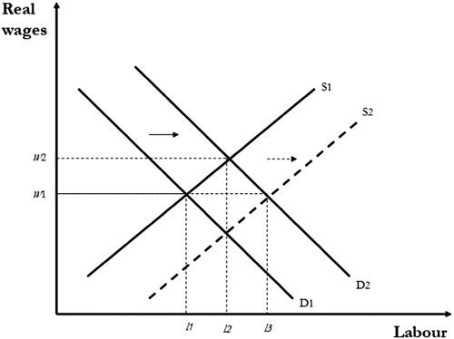
To establish profitable enterprises, settler farmers in colonial Africa needed access to fertile land and labourers willing to work on farms. While most of the land was occupied and therefore demanded ‘negotiations’ with the indigenous elites, it was the question of labour supply that posed the greatest challenge for the settler farmers. To understand how settler agriculture expanded, we have to examine how the settlers managed to solve the ‘labour problem’. According to the first strand of literature on labour supply in settler Africa, it was combinations of market forces and seasonality that ensured a steady labour supply at low wages. Fluctuations in labour demand allowed Africans to increase total income by temporarily transferring labour to the European sector without threatening their own farming operations (Barber 1960). However, in the late 1960s–1970s, a ‘radical’ interpretation of the underlying mechanisms behind labour supply in the southern settler economies emerged. The seminal works by Arrighi (1966, 1970) inspired a new strain of literature arguing that not market forces but political mechanisms were behind the witnessed labour supply at low wages. Initially, African commercial farmers played a critical role in supplying food to the growing mining sector in Southern Rhodesia and South Africa, creating labour shortages. Legislative and administrative action was taken to create a class of impoverished wage workers. Taxation alone could not solve the labour problem as the African farmer could obtain cash by selling produce to the market. So to increase the supply of African labour, the settlers successfully lobbied for land tenure policies such as the establishment of labour reserves and a reduction in the size of land available to the Africans. Thereafter, Africans were gradually relocated to the so-called ‘native reserves’ (or ‘homelands’ as in the case of South Africa) located in less fertile areas where land was typically of lower quality. The aim of the policies were, to quote Austin (2016: 317–318), ‘to restrict African land rights (whether owners, or even as tenants on European-owned land) in the hope of driving the majority of the population out of the produce markets and into the labour market’. These reserves soon became overpopulated and with the extensive nature of African agriculture this led to declining average agricultural yields. In other words, the combination of taxation and land tenure policies became a precondition for the establishment and expansion of settler agriculture (see also Cohen 1976; Bundy 1979; Phimister 1988). This classic interpretation of colonial institutions, labour supply, and real wages is depicted in Figure 1. The influx of settlers and the subsequent rise of large-scale farming shifted the demand curve outwards from D₁ to D₂ raising real wages from w₁ to w₂ and labour supply from l₁ to l₂. In settler economies (unlike the peasant economies), the colonial authorities intervened to lower the pressure on wages. The mentioned land tenure policies and the increase in taxation shifted the supply curve outwards from S₁ to S₂ leading to a higher labour supply l₃ at lower real wages w₁.

Figure 1: The impact of colonial policies on African labour supply and real wages

Note: Inspired by Frankema & van Waijenburg 2012.

The early works on Southern Rhodesia and South Africa influenced the historiography of colonial Kenya and scholars noted the many similarities between the colonies.⁵ Just as in the southern African colonies, so too did land tenure policies and taxation facilitate the creation of a labour surplus in Kenya. To quote Palmer and Parsons (1977: 243): ‘Thus by the end of the 1930s, the agricultural economy of the Shona and the Ndebele, like that of the Kikuyu and most South African peoples, had been destroyed.’ Despite a general agreement that extra-economic measures played an important role in solving the labour problem there is controversy on the degree of coercion applied by the state to solve the labour problem. On one end of the spectrum, Wasserman (1974) and van Zwanenberg (1975) maintain that illegal recruitment, forced labour, taxation, and land tenure policies were used in as late as 1950 to force Africans to work on settler farms. Other studies note that the use of forceful labour coercion declined in the 1920s. By then a deliberate neglect by the colonial administrators of African agriculture and a general favouritism of settler agriculture was enough to guarantee a labour supply (Brett 1973; Clayton & Savage 1975; Stichter 1982). Without making a distinct connection to the expansion of settler agriculture, few scholars note that forceful labour coercion was replaced by a labour control regime that made it easier to restrain and discipline workers (Berman & Lonsdale 1980; Anderson 2000). On the other end of the spectrum, a few ‘liberal’ scholars have sought to nuance the debate by emphasizing the role of non-political factors in ensuring sufficient amounts of labour. Mosley (1983) offered a detailed empirical account of the development of both African and settler agriculture in Southern Rhodesia and Kenya. The study concluded that labour coercion was used to the mid-1920s, but thereafter, the gap between labour demand and supply was filled by the private recruitment of workers from poorer parts of the colonies and by increasing the engagement of female and juvenile labour (see also Bolt & Green 2015, who reach a similar conclusion on settler agriculture in Nyasaland). According to Mosley, land tenure policies did not cause a regression of African agriculture. On the contrary, Mosley (1983) notes that certain African reserves experienced ‘Boserupian’ growth, with their yields and population densities reporting positive correlations. The debate on settler agriculture and labour went silent for almost two decades; however, recently, the ‘radical’ interpretation has resurfaced in the New Institutional Economics and African Economic History literature that tries to explain long-run developments in Africa. In the settler economies, the deliberate attempts by the colonial state to shift the labour supply-curve outward created ‘dual economies’ with persistent high levels of inequality and stunted economic development (Austin 2008; Bowden et al. 2008; Acemoglu et. al. 2001, 2010; Frankema & van Waijenburg 2012).

The contemporary literature reveals a need for re-examining the underlying mechanisms carefully before drawing conclusions on long-run development in settler societies. There are several weaknesses in the past research that has inspired this paper. Apart from Mosley (1983) none of the works mentioned explicitly study the development of the settler economy. By applying a narrow focus on labour supply, the studies are not able to convincingly tie the introduction of various labour policies to the expansion of settler agriculture. We do not know if the decline in African real wages that Arrighi (1966, 1970) finds is due to labour coercion or contractions of the settler economy. Further, while Arrighi convincingly demonstrated significant theoretical depth, he offered limited empirical evidence in support of his conclusions. To elaborate, Arrighi relied on maize figures to argue the decline of African agriculture. This is problematic as it hides any indigenous attempts to shift to cash crop farming. Mosley (1983) highlighted these concerns and offered alternative explanations for the development of settler agriculture, yet, his study suffers from shortcomings related to admittedly weak data. Two data points (1932, 1948) are used to support the hypothesis that African agricultural development followed a Boserupian path. Only a few of the districts included in his analysis (30% of the total sample) yields a positive relationship between population pressure and yields, as pointed out by Choate (1984). More severely, Mosley lacks data to support the key argument that recruited labour could close the gap between supply and demand after the 1920s. The strength of the present study lies in its consideration of both settler and African agricultural development. Further, instead of limiting our analysis to one crop, we use newly collected district-level data on African agriculture.

In the following sections, we first analyse the development of settler agriculture and then discuss the role of labour coercion.

ESTABLISHMENT OF PROFITABLE SETTLER AGRICULTURE IN KENYA

The history of European settlement in Kenya began in the early 1890s with the construction of the Uganda Railway that connected Lake Victoria to the coast of Kenya. Due to the high maintenance costs of the railway, the British government began encouraging large-scale settler agriculture to increase earnings. The settler farming community comprised three fundamentally different groups: financially strong settlers often of aristocratic origins, smaller and capital-scarce families with farm holdings that accounted for the vast majority of farms, and a few capitalized European companies mainly cultivating plantation crops such as sisal.

Sector performance

In the first two decades of European settlement, Kenya heavily relied on the mono-cropping of cereal crops such as maize and wheat, leading to low export values. In the early 1920s, however, the sector was restructured such that more settlers began cultivating high-value crops (e.g. coffee and tea). In addition, increasing areas were cultivated during this period, which has been referred to as the ‘Golden Age’ of European agriculture.⁶

From 1920 to 1930, the sector more than tripled its export earnings with an increase from £669,028 to £2,763,707 (Kenya Colony 1920–30, 1930). To better understand the effect of expansion in acreage and export on profitability, we estimate the gross annual earnings for the entire sector. We calculate the settler farm earnings by deducting depreciation expenses of agricultural machinery and annual labour, fertilizer, transport, and other transaction costs from the annual agricultural production values (Figure 2). For further elaboration on data and methods, see Appendix 1, 2, 4, and 5. We consider estimating the annual wage bill to be the most challenging task because wages accounted for the largest share of production costs. To determine annual wage costs, we reference the Kenyan archival sources for detailed employment data on the three forms of agricultural labour: tenants, monthly paid workers, and casual labour. A majority of the wage data for tenant and monthly paid labour are available in the administrative records. As is often the case with colonial statistics, the data points for female and juvenile labour are few. We interpolate data in the case of missing values. Assuming all workers received the stated minimum wage, we expect our wage bill to slightly overestimate the true labour costs, particularly since secondary sources have indicated that minimum wages were not always enforced (see Kenya Colony 1935; Kitching 1977).

Figure 2: Earnings in the European agricultural sector in pounds, 1920–45

Sources: Authors’ own calculations. Production and export values are taken from the Agricultural Department annual report 1920–45; Employment and wages are taken from the Native Affairs Department, Labour Department annual reports 1920–45 and from Mosley (1983); Import values are taken from the Annual Trade Reports 1920–45. Notes: The preferred measure uses production values for coffee, maize, and wheat and export values (deducted by 15% to take into account transaction costs) for sisal, tea, sugar, potatoes, cotton, and coconuts to calculate revenue. Our robustness check use data on export values only deducted by 15% to take into account transaction costs. In both cases, we deduct curing charges from coffee values.

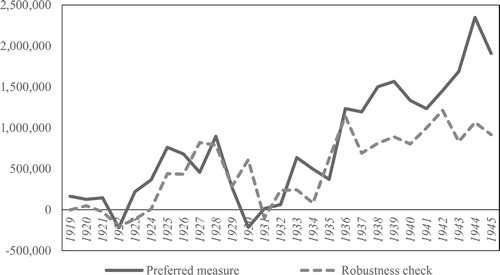
To examine the validity of our measure, we searched for officially reported annual wage bills. The Statistical Abstract (SA) began reporting agricultural wage bills in the 1950s. If we extend our time series, the estimated wage bill comes fairly close to the reported bill, with a mean difference of 1% and a maximum difference of 10% (Kenya Colony 1957–60).⁷ Another data limitation is that the total production values were inconsistently reported in the administrative records. The records indicate the production values for main crops including maize, coffee, and wheat (roughly 60% of the total production value) but only the export values for the remaining crops such as sugar and tea. To implement a solution, we use production values where available. For the crops where we lack production values, we follow Bolt and Green (2015) and use export values to proxy production values. We deduct a mark-up of 15% from the export values based on the transaction costs of exporting coffee and sisal to arrive at production values.⁸ In performing a robustness check, we calculate earnings using the deducted export values only. The robustness check shows that the use of export values slightly underestimates true earnings due to the inability to capture earnings from crops sold domestically. Our measure is therefore a conservative measure of true earnings. Figure 2 shows that the expansion in acreage and exports increased earnings. In the early 1920s, the sector transitioned from being a low-income sector to a profitable one. We observe an upward trend in profitability. The sector was, nonetheless, vulnerable to fluctuations in international demand and following the contraction of the global economy in 1920–21 and during the years of the Great Depression we see a decline in earnings mainly driven by lower coffee prices.

Labour and profitability

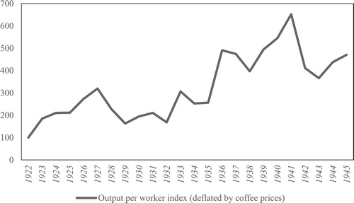
Having pinpointed the rise in profitable settler agriculture, in this section we explore the reasons underlying the expansion of earnings. First, we measure land and labour productivity in the years for which data are available. We estimate land productivity at the sectoral level for coffee and maize. Ideally, we would calculate labour productivity at sectoral level; however, the limited employment data available prevent us from doing so. Thus, instead, we calculate a ‘rough’ measure of the value of output per worker for the entire sector. To proxy real changes in labour productivity, we deflate our output series by the coffee price index as coffee was the main export commodity. As shown in Figure 3, land productivity marginally improved for coffee from 297lb of clean coffee per acre in 1920 to 314lb in 1946 (Figure 3). Maize yields per acre fluctuated around a mean of 1242lb per acre (approximately 6 bags) with no upward trend (Kenya Colony 1920–63).⁹ Labour productivity, on the other hand, did increase in the period and Figure 4 shows that increased settler profitability was largely driven by higher output per worker.

Figure 3: Land productivity for coffee and maize (measured as yields in lb per acre), 1921–44

Source: Authors’ own calculations. Data is taken from the Agricultural Department annual reports 1921–44. Note: Yields are calculated using data on European production of clean coffee and maize and European coffee and maize acreages.

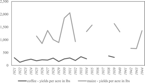
Figure 4: Labour productivity index measured as output per worker for the entire settler agricultural sector (deflated by coffee price index), 1920–45

Source: Production, export values, and coffee prices are taken from the Agricultural Department annual report 1920–45; Employment and wages are taken from the Native Affairs Department and Labour Department annual reports 1920–45 and from Mosley 1983. Notes: Labour productivity is calculated by dividing an index of value of output (deflated by a coffee price index) by the index of total employment in agriculture. The total employment measure includes both wage workers and tenants.

The shift to high-value cash crops such as coffee increased output per worker, attracting greater settler investments in agriculture. Consequently, more land was put under cultivation: in particular, land for coffee plantation alone significantly increased from 33,813 acres in 1921 to 96,042 acres in 1930 (Kenya Colony 1920–30). This shift warranted a simultaneously large increase in the number of labourers employed. The Labour Commission (1927) estimated that a coffee estate of 100 acres needed 45 full-time workers (and 80 workers during the peak season), whereas maize required only six workers per 100 acres (and an additional six during harvest). This clearly demonstrates the importance of labour access to the expansion of settler agriculture. In the case of coffee production, estimated labour demand increased from 15,216 permanent workers (and 27,050 additional workers during harvest) in 1921 to 43,510 permanent workers (and 77,351 additional workers during harvest) in 1930. Evidently, labour supply responded favourably to the increase in demand. From 1920 to 1945, the average number of monthly paid workers in agriculture considerably increased from 53,709 to 118,300 (Kenya Colony 1920–45a). It is likely that the actual number of workers employed was even higher because the employment statistics were based on labour returns submitted irregularly by employers (Tignor 1976; Mosley 1983).

ROLE OF LABOUR COERCION

African real wages

The increased output per worker should have, ceteris paribus, led to higher wages. When there is little or no government intervention in the labour market, we expect real wages to equal the marginal product of labour. In our first step to understanding the role of labour coercion in expanding the settler agricultural sector, we calculate African real wages using Allen’s (2009, 2013) subsistence basket approach. The approach divides an adult worker’s annual income by the costs of a family subsistence basket and expresses real wages as a welfare ratio. Prior to the consolidation of wages in the late 1950s, the value of free meals and housing constituted a large part of the total wage. To take this into account, we follow the literature, and include value of rations in the total income measure. Due to lack of data, we are not able to include the value of housing and our total income measure slightly underestimates true income. For further elaboration on welfare ratio, see Figure 5 and Appendix 3.

A welfare ratio of one indicates that the worker and his family are barely surviving, whereas a ratio greater than one suggests that the family lives above the subsistence level. Still, the measure is subject to an important caveat: it assumes that an agricultural worker was a full-time employee. By contrast, agricultural workers in Kenya were generally employed under contracts of 3–6 months (Economic & Finance Committee 1923). For that reason, we do not expect the measure to adequately estimate the actual living standards for wage workers and their families. Instead, we use the measure as a proxy of the development of the purchasing power of wages.

Real wages were the highest in the first decade of settler agriculture development, with a welfare ratio of 2.72 in 1914 (Figure 5). In fact, this ratio was relatively high at an international level and was almost at par with the urban welfare ratios of Ghana (Accra) and Sierra Leone (Freetown).¹⁰ Yet, a general trend during the period was the stickiness of nominal wages and the rise in rural prices, which caused real wages to decline first and then remain stagnant. More specifically, during the period 1912–45 the welfare ratio of a worker and his family was marginally greater than one (the mean was 1.38), indicating limited welfare gains from employment. This trend could possibly indicate that policies aimed at increasing labour supply became more coercive over time, forcefully creating a labour surplus large enough to ensure unlimited supplies of labour at low wages.

Taxation

To investigate the level of coercion, we first analyse Kenya’s taxation policies. In 1902, all African Kenyans were obligated to pay a hut tax, a uniform tax payable by the owner of a hut. If a male older than 16 years did not own a hut, he was required to pay a poll tax of the same amount instead. To determine the effect of taxation on labour supply, we calculate the per capita tax pressure for the benchmark years of 1915, 1920, and 1930 by dividing the annual direct tax by the daily wage of a rural male worker.¹¹ In 1915, a rural male worker was required to work 11 days to incur annual taxes. In 1920, the required workdays remarkably increased to 60 days. In 1922, a few years before the development of the settler farming sector, colonial authorities decided to reduce the hut/poll tax from 16 to 12 Ksh., which was maintained throughout the inter-war period (Kenya Colony 1920–45b). As a result, in 1930, the tax pressure declined to 23 days.

Still, per capita tax pressure does not provide a complete overview of taxation for the following three reasons. First, the decline in tax pressure could have been offset by efforts to enhance the enforcement of tax payments. Second, differential local tax rates could have been used to increase tax pressure in labour-supplying areas. Finally, indirect taxes might have raised the overall tax burden. The colonial administration constantly debated ways to achieve more ‘efficient’ tax collection systems and methods, such as having chiefs or settler farmers collect taxes (van Zwanenberg 1975). In 1923, shortly before the expansion of settler agriculture, the total value of direct African taxation was £575,000, but by 1928, the value had dropped to £564,000 and further to £530,000 during the Great Depression in 1935 (ibid). This alludes to a population decline, widespread tax evasion, or a decline in the sales of produce making it harder to generate income. In general, the national tax rate applied to ethnic groups throughout the colony, although there were a few exemptions. The colonial officers initially believed the Masaai people to be wealthy; thus, they were required to pay a higher tax of 20 Ksh. Despite the higher taxes, the Masaai people generally did not work on settler farms (Stichter 1982). Few groups residing in less developed districts, mainly on the coast and in northern Kenya, paid a lower rate of 6–8 Ksh. A majority of the Africans, including ethnic groups that supplied labour paid a uniform rate of 12 Ksh. No indirect tax was levied on locally produced goods during this period. Custom tariffs did apply to goods imported into the colony, although we find no systematic trend for changes in the tariffs. In 1931, an increased duty was imposed on imported luxury goods such as vehicles, tea, ale, and beer, items which were mostly consumed by Europeans. Three years later, the tariff on textiles and bicycles increased, which may have impacted the African population. There was no further increase in the tariffs in the subsequent years (Kenya Colony 1920–45b). The decrease in tax level in 1921 may have caused a temporary drop in labour supply given the reported shortages in 1923 and 1924. Nevertheless, any effect on labour was short-lived and despite the increase in tariffs on textiles and bicycles, no shortage was reported in the remaining years (Kikuyu Province 1920–37), indicating a rather weak link between labour supply and taxation.

Type and origin of labour

As argued in previous research, taxation alone was insufficient to make Africans work for low wages. Produce sales supplied Africans with sufficient cash to pay taxes. In fact, it was the combination of taxes and a politically induced decline in African agriculture that facilitated the workforce expansion. This section explores the linkages between labour supply and the development of the African agricultural economy. We begin by examining the origin of workers employed on settler farms. According to Figure 6, short-term wage workers and tenants accounted for a majority of the labour force, although the share of migrant workers seemed to decline.¹²

Figure 5: Welfare ratio – based on the annual income of an adult male agricultural worker, 1912–45

Source: Authors’ own calculations. Wages are taken from the Blue Books 1912–30, Native Affairs Department 1930–45, and Mosley 1983. Rural commodity prices are taken from the Central/Kikuyu and Nyanza Province annual reports 1912–45. Prices for imported are taken from the Blue Books and Trade Reports 1912–45. Notes: (1) Standard methods are used to calculate the welfare ratio (see Frankema & Waijenburg 2012; Allen 2013; de Haas 2017). (2) Caloric content is taken from Latham 1997. (3) Similar to de Haas (2017), we include beans and we allow the family to choose the cheapest grains variety (maize, millet or sorghum). Following Frankema and van Waijenburg (2012), we add 10% to the cost of the basket to take into account firewood/charcoal and candles, as data for these items is missing. In addition, a 5% mark-up is also added to account for the cost of maintaining a rural dwelling.

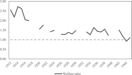
Figure 6: Labour composition on European farms, 1928–37

Sources: Data on tenant and short-term workers is taken from the Agricultural census 1928-1937. The number of long-term workers (referred to as ‘contracted workers’ in the colonial records) is taken from the Native Affairs Department annual reports 1928-1934; for 1931, 1935. For 1936 the source is Fearn 1961. Notes: (1) For 1931, 1935, and 1936, we only have data on long-term workers from the Nyanza Province. This should not cause interfere with our results and conclusions, as the vast majority of long-term workers came from the Nyanza Province. (2) Due to lack of data, the number of tenant labourers is interpolated using a log-linear approach for the years 1930, 1931, 1935, and 1937. (3) Tenant workers are not reported separately from wage workers before 1927 (Mosley 1983). We are therefore not able to extend our time-series back. Another concern is the manner in which long-term workers are recorded: these are reported as ‘contracted labour’ but the administrative reports do not distinguish between contracted labour in industry and in agriculture. Thus, we might be overestimating the role of migrant labour slightly. This does not affect our conclusion, that short-term and tenant labourers were the most important sources of labour.

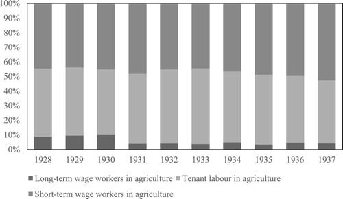
Figure 7: Administrative map of Kenya

Source: ILO (1972) ‘Employment, incomes and equality’ Note: ▭ Main labour supplying area.

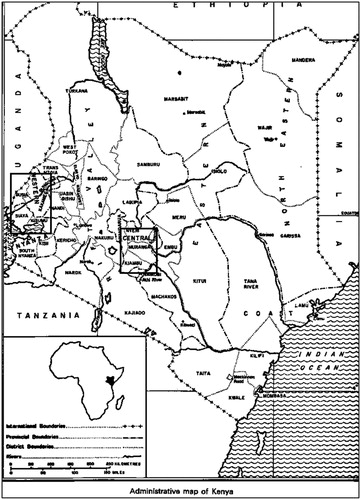
A majority of the tenants were from the populous Kikuyu reserves;¹³ for instance, roughly two-thirds of the tenants were from Kiambu and Fort Hall (Leys 1975; Tignor 1976; Stichter 1982; Kanogo 1987). Kikuyu tenants settled on European farms in the Central Province and farms in Nakuru and Laikipia in the Rift Valley Province. The remaining one-third belonged to the Kamba and Nandi ethnic groups that lived in close proximity to remote farms in Uasin Gishu and Trans Nzoia in the northern region of the Rift Valley (Stichter 1982). The other dominant labour pool comprised short-term workers who were employed on a monthly basis and would generally work 2–6 months a year. Similar to tenants, a majority of the wage workers were from Kikuyu reserves (see Kenya Colony 1928–45; Stichter 1982). Further, while short-term workers and tenants came from areas close to European farms, long-term workers were migrants from the Luo and Luhya ethnic groups in the Nyanza Province of western Kenya (Figure 7). Year-long labour requirements were higher for sisal and tea than for coffee; consequently, migrant workers would seek employment in these sectors (Fearn 1961).

Labour supply and the African agricultural economy

To further our discussion on labour coercion, we examine the trends in African agriculture. Unlike Tanganyika and Uganda, data on African agriculture in Kenya are rather scarce. Kenya’s national administrative records contain almost no data on production prior to the 1930s, when colonial officers began reporting a few estimates on African production. The export values of African agriculture are available from 1922 and increased from £176,000 in 1922 to £447,495 in 1945 (Kenya Colony 1922–24; 1935–45).¹⁴ Maize was mainly produced in the labour-supplying Nyanza and Kikuyu reserves and its export value increased from £73,000 in 1922 to £100,000 in 1925. However, the national records do not offer regional-level data. To capture regional-level trends, we carefully examine province- and district-level annual reports. In the remainder of this section, we calculate the average earnings from sales of produce per household. Positive earnings indicate that, on average, families produced more food items than needed for their own consumption. Further, we examine if earnings were sufficient to pay taxes (during this period, the tax level was 12 Ksh. per hut). Low and/or declining earnings will lend support to the standard interpretation of labour supply in settler economies. On the other hand, earnings greater than the tax level indicate that farmers worked for wages, not out of necessity, but to enhance the possibilities for household consumption. We first examine Nyanza Province, the area which supplied migrant workers.

In Nyanza, maize was the most important food and cash crop, followed by hide, groundnuts, and sesame. In 1922, income from agricultural produce sales was merely 4 Ksh. per household, which was a significantly low value to levy the annual tax. Nevertheless, we see an upward trend in earnings thereafter. In 1935, the average earnings per household increased to 7 Ksh. per household, further increasing to 19 Ksh. in 1940 and 21 Ksh. in 1945.¹⁵ From 1936, on average, income was sufficient to pay taxes. Unfortunately, the data do not allow us to further disaggregate earnings. We note that the rise in income was driven by the sale of maize and hide, products which were also produced in labour-supplying areas in central and north Nyanza. Low agricultural earnings reported in the 1920s combined with the pressures to pay taxes could explain the migrant labour supply until the mid-1930s. Migrant workers, nevertheless, accounted for a small and declining fraction of the total labour supply (around 10%).

Next, we explore the agricultural economy of the Kikuyu reserves, which, by far, had supplied the largest share of labour. Initially, the main crops grown for consumption and sales in the reserves were maize, potatoes, and beans, of which maize was the dominant crop (Kikuyu Province 1929–30). The first consistent estimates of sales for food items were reported from 1927. Unfortunately, we lack total earnings from agricultural products sales. If we examine maize, in 1927,¹⁶ 40,000 tons of maize was exported with high per capita earnings of 6.25 Ksh. Yet, if we examine the years leading up to the Great Depression, it is possible to paint a picture of a decline in Kikuyu agriculture. No sale of food items from the Kikuyu reserves was reported in 1929 and 1930. The literature (e.g. Brett 1973; Stichter 1982) has suggested that colonial policies that systematically favoured European over African producers or the outmigration of labour led to the decline in sales. By contrast, the administrative reports attributed the decline to unfavourable weather conditions and locust outbreaks (Kikuyu Province 1928–29). Available empirical evidence has indicated that the drop in sales was, in fact, transitory. In 1932, a detailed economic survey of the Kikuyu reserves was conducted by the District Commissionaire of Kiambu. According to Fazan (1932), maize production recovered total sales amounting to 36,905 tons and a corresponding value of 101,489 pounds. As Table 1 shows, contrary to assumptions made in the literature, household income from produce sales was higher in the labour-supplying areas (Kiambu and Fort Hall) and earnings were sufficient to pay the annual taxes.

Table 1: Estimated average value of total produce per household in the Kikuyu Proper Native Reserves, 1932

	Value of produce per HH
Per household in:	Consumed (Sh.)	Sold (Sh.)	Total (Sh.)
Kiambu	121	107	228
Fort Hall	139	52	191
Nyeri Native	160	28	188

Source: Kenya Land Commission 1934 – CAB/24/248

The case of wattle bark production best illustrates agricultural development in Kikuyu. Today, wattle bark is considered a minor raw material in the leather industry.¹⁷ However, at the time, households used it as firewood and building material and importantly, sold it as a cash crop for exports (Kikuyu Province 1932). Wattle bark production in the Kikuyu reserves reported a take-up rate of as high as 75% of households in Kiambu, Fort Hall, and Nyeri (Cowen 1978). Similar to food production, a majority of wattle bark production was done in areas with high labour force participation rates (Table 2). This pattern of high participation rates in the labour market and investments in wattle bark production lasted throughout the colonial period. Data from the 1960 Sample Census of African Agriculture show that 30 years later, Kiambu continued to report the highest share of wattle-producing households (47.6% compared to Embu’s 3.1%) (Kenya Colony 1960).¹⁸

Table 2: Acreage under wattle bark and labour force participation rates in Kikuyu Province by district in 1930

Area	Wattle bark acreages in 1930	Labour force participation rate in 1930 (percentage of able-bodied males)
Kiambu	6,119	69.0%
Fort Hall	448	35.4%
Nyeri	120	36.6%
Embu and Meru	1	Embu: 15.7% and Meru: 25.9%

Source: Authors’ own calculations. Wattle bark acreages are taken from the Agricultural Census 1930. Data on population and employment is taken from the Native Affairs Department annual report 1930.

To carefully analyse the importance of wattle bark to Kikuyu households, we estimate the earnings per household (Table 3) using the population data from wattle-producing districts in the Kikuyu reserves (i.e. Kiambu, Fort Hall, and Nyeri). We deduct associated labour costs because of the use of hired labour to strip the tree barks, as mentioned in Stichter (1982) and Cowen (1975). It is possible that the resultant true income is underestimated because we assume that all households produced wattle, whereas in reality, about two-thirds of the households did so. The estimates reveal rather low earnings from the wattle sales in the export market.¹⁹ Nevertheless, these earnings were sufficiently large to impact labour supply as, on average, households in labour-supplying areas earned sufficient income from produce sales to be able to pay taxes.

Table 3: Estimated wattle bark earnings per household 1929–45

Year	African produced wattle bark in Kikuyu Province	Estimated wattle bark earnings per household	Nominal 30-day wage for a male worker in agriculture
	Export value in pounds	Value in shillings	Value in shillings
1929	35,000	6.5	8–12
1930	42,000	20.1	12
1931	72,521	14.1	13
1932	78,810	22.5	10
1933	46,600	12.2	6–10
1934	51,658	14.5	6–12
1935	44,570	11.5	9
1936	48,748	19.3	6–12
1937	45,483	13.3	11
1938	29,357	4.8	8–12
1939	72,846	14.6	8–12
1945	89,448	15.1	10–16

Source: Authors’ own calculations. Wattle bark figures are taken from the Native Affairs Department annual report 1938–1948. Years 1936 and 1937 are taken from the Central Province annual report. Nominal wages 1929, 1930, 1933, 1934, 1936, 1938, and 1939 are taken from the Native Affairs Department annual reports. 1931, 1932, 1935, and 1937 are taken from Mosley (1983). Population data is taken from the Kikuyu Province annual reports except for years 1925, 1938, and 1939 where data is taken from the Native Affairs Department annual report.

Notes: (1) To calculate earnings per household we use the total population of the wattle bark producing districts Kiambu, Fort Hall, and Nyeri. We obtain estimates of household size from S.H. Fazan’s 1932 economic survey of Kikuyu proper (CAB/24/248 Kenya Land Commission Evidence, I, 979) (2) To estimate the costs of hired labour, we assume that 10 trees could be stripped per day per household (see United Nations 1977). We further assume that a farmer would have a maximum of 100 trees. 100 trees per farmer seems reasonable, as Fazan (1932) estimates that households would plant between 0.11 to 0.37 acres of wattle and we know from colonial Natal, that one acre could have around 400–450 trees (Sherry 1971). It follows, that a household would need to hire labour for 10 days to strip bark. To calculate the costs of hired labour, we assign the lowest daily agricultural wage to the number of workdays. (3) Population figures are unusually high for 1931 causing a drop in earnings. The high population rate could be due to a mistake in the colonial recordings.

Another indicator of increased commercialization in the labour-supplying areas is the growth in African-owned shops in the 1920s. In Fort Hall alone, the number of shops increased by almost 70% (from 144 to 208) during 1927–28 (Kikuyu Province 1928). The pattern of agricultural investments and commercialization in the Kikuyu reserves persisted for several decades. The cultivation of permanent crops is typically considered a suitable indicator for agricultural investments and thus, a sign of progress. In 1960, 12% of Kikuyu reserves were under cultivation for permanent crops in comparison to the limited 1.4% in Nyanza. These values highlight stark intra-reserve diversities: in Kiambu, the labour-supplying Kikuyu reserve, 38% of the land was under cultivation for permanent crops, whereas in Embu and Meru, areas which supplied less labour, the rate of land under cultivation was merely 5 and 7%, respectively (Kenya Colony 1960).

These findings pose an important question: if commercialization was on the rise, why did farmers work on European estates? Low earnings combined with the need to pay taxes could explain part of the labour supply for migrant workers. For the bulk of labour, however, the answer probably lies in a combination of seasonality and deeper integration in the cash economy. The agricultural calendar for crops grown in Kikuyu suggests that labour could be freed from smallholder agriculture during the peak coffee season from late October to January (Table 4).

Table 4: Agricultural calendar for Kikuyu grown crops and coffee

Activity/month	Jan	Feb	Mar	Apr	May	Jun	Jul	Aug	Sep	Oct	Nov	Dec
Kikuyu grown - cereal crops	Harvest short rain crops (e.g. maize) Long rains Harvest long rain crops Plant short rain crops Oct: Circumcision Plant crops for long rains (e.g. maize, beans, potatoes)
Settler grown coffee	Prune Coffee harvest
Kikuyu grown wattle bark	Wattle bark stripping Wattle bark stripping

Sources: For Kikuyu grown crops see the Native Affairs Department annual report 1924: 49; Kenyatta 1938; Sticther 1982. For coffee and wattle bark see the Native Affairs Department annual report 1924: 49.

TOWARDS AN ALTERNATIVE EXPLANATION

Policies to shift the labour supply-curve outward do not appear to have played a role in the expansion of settler agriculture in Kenya. Instead, we grant support to the previous literature noting that the ability to control available labour was more important. This section explains the role that tightened labour control played in lowering both wages and transaction costs allowing the settler to raise their profit share. Settler farmers were faced with numerous challenges. The cultivation of mono-cereal crops such as maize and wheat was not profitable because of the high transport costs (Tignor 1976; Mosley 1983). At the same time, capital was costly. Since settlers operated in a high-risk environment, they preferred labour-intensive production methods even for large estates (Mosley 1983). Initially, both wages and the transaction costs of seeking and retaining workers were high. Settlers had to pay high fees to costly and inefficient private recruiters (Berman & Lonsdale 1980). Further, contract enforcement costs were high as workers would often desert. These costs were brought down with the introduction of two new laws. In the late 1910s, shortly before the European sector expanded, two policies that limited African mobility and raised the workload of the tenants were introduced, that is, the Resident Native Labour Ordinance (RNLO) and the Registration of Natives Ordinance (also known as the ‘pass law’). These laws would make the shift to high-value cash crops even more profitable.

In 1919, the RNLO was passed and prohibited fixed-rent tenancy. The 1919 ordinance and those that followed drastically altered tenants’ rights. Prior to the ordinance, the African tenants were able to negotiate fairly good conditions; some would work a limited number of days in return for tenancy, while others paid rent. The area of land for grazing and cultivation was at least 5 to 6 acres, and a family could own and maintain large herds of livestock (Furedi 1972; Stichter 1982). However, following the 1919 ordinance, tenants were no longer allowed to pay rent in cash and were instead turned into ‘rent labourers’. A male tenant would have to give a minimum of 90 days’ work per year and, in return, receive a low 30-day ticket wage.²⁰ Then, in the late 1930s, the 1919 ordinance was augmented to provide settlers with even greater control over the tenants. Consequently, the number of work days increased to 240–270 days per year. At the same time, the area of land for cultivation decreased to one acre and the number of livestock to a maximum of 10–15 sheep. Settlers’ control over tenants was further strengthened by the decision to shift the responsibility of overseeing tenant ordinances from the colonial administration to settler-dominated district councils. Further, no compensation was offered to offset the income loss from the restricted cultivation and livestock.

An important question to explore here is why the tenants did not return to the reserves despite the worsening conditions. The tenants had after all voluntarily entered into contracts with the settlers and as we argue an increased commercialization was taking place in the Kikuyu reserves. First of all, tenants who could return did so. In 1928, the Agricultural Census presented for the first time the number of residents, of whom 32,969 were male tenants (Kenya Colony 1928). In 1936, due to the outmigration of tenants, this number declined to 24,872 (Kenya Colony 1936). However, not all tenants could return. One of the few studies on Kikuyu tenants is Furedi’s (1989), which found that the Kikuyu land rights system was central to tenants’ ability to return to the reserves. Some tenants lost their land rights, often to other family members, while they were away from the reserves. A large proportion had never owned land and lived as ahoi (labour tenant or serf, Kikuyu) on Kikuyu landowners’ farms prior to migrating to European land. A smaller proportion cited bad relationships with the chiefs as a reason for not returning to the reserves.²¹

Due to the immobility of the remaining tenants, settlers could extract a higher number of work days. The ability to use tenants as semi-permanent labour ensured a timely supply of labour that could be called upon when needed drastically lowering the transaction costs of finding labour. Despite this, the supply of labour was still insufficient. This was particularly the case for the burgeoning coffee sector and during the harvest season, short-term workers from nearby reserves were hired to fill the gap. On the one hand, employing short-term labour during peak seasons allowed for easier monitoring since they were hired to perform specific tasks. On the other, unlike migrant or tenant workers, local short-term labour could easily desert the farm, leading to high contract enforcement costs. As a result, strong penalties were enforced as part of the labour contracts under the pass laws implemented in 1921, which forbade Africans from leaving the reserves without a passport. The pass, commonly referred to as kipande (card, Kiswahili), listed personal details, previous employer, and the wage earned. The system enabled the settler community to better control the wage level and to retain workers more easily since deserters could be traced. We reference data on the number of deserters to illustrate the effectiveness of the law in reducing transaction costs. In 1921, when the law was implemented, 3595 deserters were reported. Of these, 77% were punished under the new law. However, in the year following the implementation, only 149 cases were reported (Leys 1924). Importantly, while the deserter problem did not disappear with the implementation of the law,²² its levels did not increase to those prior to 1921.

The decrease in transaction costs was not the only ‘advantage’ of the restricted mobility of Africans. Lowered mobility also implied a reduction in the bargaining power of the African worker as settlers were faced with less competition to recruit and retain workers placing a downward pressure on nominal wages. The stabilization of the wage combined with the steady supply of cheap tenant labour lowered the wage bill. With the shift to high-value cash crops raising the value of the output per worker, settlers could capture a higher share of the surplus value.

CONCLUDING REMARKS

Literature on Africa’s economic developments has cited the presence of settler agriculture to explain past and present low living standards and high inequality in Africa’s former settler economies. In the 1970s, a consensus emerged among ‘radical’ scholars that to expand settler agriculture the colonial state intervened in the markets for land and labour to ensure the settlers a steady supply of cheap labour. More specifically, land tenure policies and taxation eroded earnings from the sales of African produce creating unlimited supplies of labour at low wages. This interpretation of labour supply in settler economies has influenced a new strain of literature that seeks to explain long-run poverty, inequality, and political instability in Africa. However, the ‘radical’ literature suffered from empirical shortcomings and failed to directly link the introduction of various labour policies to the performance of the settler agricultural sector. Consequently, we are not able to know whether declines in African wages can be attributed to colonial policies or to contractions in the settler farm economy. We contribute to the historical literature on labour in settler economies by empirically investigating the underlying causes of the expansion of settler agriculture using Kenya as a case.

To examine whether colonial policies facilitated the expansion of settler agriculture, we calculate both settler farm earnings and African real wages. The two measures reveal a paradox: settler profitability and employment rose while African real wages declined. To examine the role of colonial policies, we correlate the two measures with taxation and developments in the local African agricultural economy. Doing so, we do not find support for the classic interpretation that declines in African agriculture and taxation can explain the steady supply of labour at low wages. On the contrary, we find that the bulk of labour came from native reserves becoming increasingly more commercialized in the period. A combination of seasonality and deeper integration with the cash economy seem to explain a majority of the labour supply.

The rise in settler profitability can instead be explained by a shift to high-value cash crop production coinciding with tightened labour control. The shift to coffee and tea raised the value of output per worker, yet this did not manifest itself in higher wages. This can be explained by the emergence of a labour control regime that placed downward pressures on both transaction costs and wages enabling the settler to capture a higher share of surplus value. Our results conquer with past and present literature that has linked poverty and declining living standards to the expansion of settler agriculture. Our findings need not be unique to Kenya. Similar measures were taken to reduce labour mobility in for instance South Africa and Southern Rhodesia (see e.g. Nattrass 1991; Rennie 1978) and we propose that these measures might have played a more important role than policies to raise labour supply. Still, more research on labour control and settler agriculture is needed to understand not only the political economy of settler farming in Africa but also to explore how white settlement affected the economic opportunities and freedoms of the indigenous African populations.

Disclosure Statement

No potential conflict of interest was reported by the authors.

Additional information

Funding

We acknowledge funding from the Swedish Research Council [Dnr: 2014-1509].

Notes

2 Mosley (1983: 5) defines a settler society as ‘a country partly settled by European landowner-producers, who have a share in government, but who nonetheless remain a minority of the population and who in particular remain dependent, at least for labour, on the indigenous population’.

3 For instance, Africans were prohibited from cultivating high-value cash crops (e.g. coffee, tea, and pyrethrum).

4 There is a rich literature on transaction costs and labour contracts in pre-industrial Europe; see for instance Acemoglu & Wolitzky 2011; Domar 1970; Fenoaltea 1984.

5 Key works include Clayton & Savage 1975; van Zwanenberg 1975; Stichter 1982; Mosley 1983 ; Berman & Lonsdale 1992.

6 See Tignor 1976 and Mosley 1983.

7 For 1956, 1957, and 1958, our wage bills are £676,697, £873,118, and £402,521 greater than the SA-estimated £7,800,000, £8,400,000, and £8,700,000, respectively. On the other hand, for 1959 and 1960, our wage bills are £93,513 and £452,904 lower than the £8,600,000 and £10,000,000 estimated by SA.

8 The 15% mark-up is based on the sea freight and insurance costs of exporting coffee and sisal to London. The mark-up overestimates the costs of crops sold nationally or within the region.

9 Yields are calculated using data on the production of clean coffee by Europeans and the European coffee acreages.

10 See Frankema and van Waijenburg 2012.

11 We adopt the direct tax level from Mosley 1983 and Berman and Lonsdale 1980 and calculate daily rural wages by dividing the official 30-day ticket wage by 30 days.

12 The literature on labour in Kenya referred to short-term workers as ‘casual labour’, ‘short-term migrant labour’, and ‘migrant labour’ (see van Zwanenberg 1975; Stichter 1977, 1982). To avoid confusion, we define workers on 30-day ticket contracts as ‘short-term wage workers’, workers employed under long-term contracts of more than six months as ‘long-term wage workers’ or ‘migrant labour’, and workers hired on a daily basis (e.g. coffee pickers) as ‘casual workers’. The colonial administration first began segregating tenants from wage workers in 1928; thus, accurate data are available for a few years.

13 Meru, Embu, and Nyeri were also a part of the Kikuyu reserves, although these regions provided fewer tenants.

14 Few scholars have referenced this increase in export values to argue that African agriculture did not decline in Kenya (see Berman & Lonsdale 1980; Mosley 1983).

15 These values are calculated using the population and agricultural sales data from the annual reports of Nyanza Province. African population data in the colonial era are subject to numerous limitations (Frankema & Jerven 2014); as a result, our estimates may also suffer the same biases. We use the official number of household members reported in the census data in Nyanza’s annual reports (3.23 members on average).

16 See Kenya Colony (1927) (Kikuyu Province, 1934-48)

17 Extracts from wattle bark are used as a tanning agent to produce leather from skin and hide.

18 In the 1950s, the production of wattle bark was replaced with that of other cash crops such as coffee, tea, and pyrethrum.

19 The export values for wattle bark remained fairly stable over the period, while the population size increased by 2%, creating downward pressure on household earnings from the crop (Kenya Colony 1920–45a).

20 The 30-day ticket wage for tenants was, on average, half of the 30-day ticket wage for a wage worker.

21 See Furedi 1989 and Lonsdale 1992.

22 Correspondence from the Chief Registrar of Natives revealed that, in the 1940s, the government remained active in tracing deserters and in issuing warrants of arrest (Kikuyu Province 1934–48)

APPENDIX 1

Data sources
European agricultural production and exports

Production and export values are taken from the Department of Agriculture annual reports 1920–45.

Wages

30-day ticket wage

Where possible, we refer to district wages and/or sector-specific wages as opposed to the more superficial wage data in the Blue Books. For the years for which we have district- or sector-specific data, we estimate the weighted (by employment share) average wages. District wage data is available in the Native Affairs Department’s annual reports for years 1923–25, 1927, 1928, 1930, and 1936. For 1920, 1921, 1933, 1934, and 1937–39, we use nationwide data on agricultural wages also from the Native Affairs Department’s annual report. We employ data from the Blue Books for 1926 and the Labour Department’s annual report for 1944 and 1945.

Where we have reported minimum and maximum wages, we calculate averages using a log-normal distribution that assigns greater weight to the lower value. For missing values, we interpolate data using the log annual difference (growth/decline) and then add the percentage to each year: ln (y1/y0)/n. Years 1922–25 are interpolated using a log-linear formula. Note that female wages are unavailable at the district level. At the national level, nevertheless, we use data on female wages for 1927, 1928, 1938, and 1955 from the annual reports for the Native Affairs Department and the Labour Department. For the remaining years, we estimate the female wages, assuming a constant male–female wage ratio. Juvenile wages are available for 1901–02 from the Blue Books and for 1927, 1928, 1938, and 1955 from the annual reports of the Native Affairs Department and Labour Department. For the remaining years, we estimate the juvenile wages, assuming a constant male–juvenile wage ratio.

Tenant wage

Data on tenant male wages are taken from the Native Affairs Department’s annual report for 1927–29, 1933–39, and 1944. For 1921–26, we extrapolate by assuming a constant ratio for male 30-day ticket wages to male tenant wages. We do not have a wage for female tenants and we estimate the wage using the male-to-female 30-day ticket wage ratio.

Daily wage

We lack data for daily paid (casual) wages. To solve, we estimate daily wages by dividing the lowest 30-day ticket wage (excluding ratios) by 30 days.

Food allowances

We include the value of food in our total wage measure. Food allowances are taken from Mosley (1983) for the years 1913, 1925–33 and 1945. Information for 1934 is taken from the Agricultural Department annual report. We assume that the value of food allowance was held constant for the years where no change is reported.

Employment

Data on male, female, and juvenile workers employed on 30-day tickets are taken from the Agricultural Census for 1921–34, 1936, 1938, 1941, 1942, 1944, and 1945. Data for 1937 are from the Blue Books. We interpolate data on male workers for 1935, 1939, and 1940; female workers for 1935–44; and juvenile workers for 1935–42.

Production costs: fertilizers and insecticides

We use import values for fertilizers and insecticides, the data for which are taken from the annual trade reports for 1921–45. A 20% mark-up is added to arrive at retail prices.

Agricultural machinery and tools

Data on agricultural tools and machinery are taken from the annual trade reports for 1921–45. A 20% mark-up is added to arrive at retail prices.

Transport costs

Railway rates and distance measures from the railhead to Mombasa are taken from the Kenya Railways Corporation’ Administration Reports. The files are available at the Kenya National Archives. The railway rates for maize are taken from the Colonial Office’s annual report for 1920, van Zwanenberg (1975) for 1927, and Mosley (1983) for 1933 and 1943.

Railway rates were generally reported when a rate decrease or increase was implemented; thus, the rates are not available for all years. Nevertheless, it seems fair to assume that the railway rates remained constant for the years in which no new rate was introduced.

Rural prices

The national colonial records provide only urban retail prices. To collect rural prices for the calculation of African real wages, we collect data from the provincial and district annual reports from the most populated regions (Kikuyu and Nyanza), which also supplied a majority of the labour. We lack the rural price data for imported goods (i.e. sugar, salt, soap, and kerosene) and are therefore unable to calculate a rural–urban price difference for these goods. Nevertheless, data from Uganda (see de Haas 2017) have confirmed that the prices for imported goods were similar between the rural and urban areas. Consequently, we use the urban retail series for all imported goods: beef, cotton, sugar, salt, petroleum, and soap.

APPENDIX 2

Earnings calculation for the settler agricultural sector

To calculate settler agricultural earnings (‘profitability’), we use the standard principles of a financial income statement:

Revenue £

Expenses

Wages

Production costs

Depreciation expense

Transport costs

Other transaction costs

Total expenses £

Gross earnings £

 

Revenue

Total revenue is calculated by multiplying production values with producer prices. Production values are generally available for coffee, wheat, and maize, which constituted 60% of the production value. We rely on reported export values for the remaining crops. Depending on the crop, this could lead to both the under- and overestimation of true earnings. We overestimate the earnings for crops sold in the overseas markets. Further, our values for true earnings are underestimated for domestically sold and exported crops (e.g. sugar) because we are unable to account for domestic sales. We deduct a 15% mark-up from the export values. This mark-up is based on the calculated transaction costs (the difference between the sales price in Nairobi and London) for coffee and sisal which included storage in Mombasa, insurance, and sea freight to London. This measure is conservative as it overestimates the transaction costs for crops sold domestically or regionally. We use the production values of the following crops: coffee, maize, and wheat. We use export values for tea, sisal, sugar, pyrethrum, coconut, beans, and potatoes. In performing a robustness check, we calculate the earnings using only the export values.

Wages

To obtain the annual wage bill, we multiply wages by employment figures for all categories of agricultural workers. If data for minimum and maximum wages are reported, we calculate an average using lognormal distribution (biased towards the minimum).

We calculate the wage bills for the following categories of workers:

• male, female, and juvenile workers employed on 30-day ticket contracts;

• male, female, and juvenile workers employed on tenant contracts; and

• male, female, and juvenile workers employed as daily workers.

30-day ticket workers

We multiply the number of 30-day ticket workers employed each year by the stated 30-day ticket wage.

Tenants

For tenants, we lack information on the number of days worked per year. Thus, to assign an annual number of work days, we use the number of days that a tenant is required to work as per the Resident Native Labour Ordinances (RNLO): 90 days from 1921 to 1939 and 270 days thereafter. Secondary sources have suggested that the wives and children of male tenants would also work during the harvest and planting seasons. Thus, we assign 60 days of work per year for this group of workers (see the Labour Department’s annual report 1945).

Daily workers

We multiply the number of daily labourers employed each year with the estimated daily wage.

Production costs

Apart from labour, production costs included those for fertilizers and insecticides. We deduct the total annual value of these costs.

Depreciation expense

Depreciation expenses are calculated from the total value of agricultural machinery and tools.

We deduct the cost of acquiring fixed agricultural assets by subtracting a depreciation rate. We use a straight line depreciation formula. The lifetime of agricultural machinery is set to four years, which is consistent with the contemporary lifespans used in accounting for African countries (see Ernst & Young 2017). See the following example:

Assuming the purchase cost of machinery is £50,000,

4 years of useful life = 25% depreciation rate per year

25% depreciation rate * £50,000 = £12,500 annual depreciation.

Transport costs

We calculate the costs of transporting goods from the railhead in a given district to Kilindini Harbour in Mombasa. We estimate transport costs for the following crops: coffee, maize, beans, cotton, sugar, tea, wheat, barley, oats, potatoes, sisal, and pyrethrum.

To account for the different locations of settler farms, we calculate transport costs as a weighted sum (by quantity in a given area). The transport costs are first calculated at the district level, as follows:

Transport cost_d= railway rate_c * distance_d * production volume_cd,

where c = crop and d = district.

Next, we calibrate the district-level transport costs to arrive at a single transport cost for the entire sector. To calculate the weighted averages, for all years, we use data on European production by district, distance measure, and railway rate for each crop. Data on European production at the district level are available only for 1920, 1922, 1930, 1934, and 1936. We use three steps to estimate the production volumes per district for the missing years. First, we calculate crop shares by district for the years in which data are available. Second, we interpolate data for the missing years to determine the district-level crop shares for all years. Finally, we use the total production volume at the national level and the estimated crop shares at the district level to assign production volumes to each district. Owing to the lack of data, we are unable to calculate the costs of transporting from the farm gate to the railhead.

The total annual transport costs, on average, were 6% of the total production value, which is marginally lower than that in landlocked Nyasaland, where transport costs were 10%, a rate that has been said to be the highest in Southern Africa (Bolt & Green 2015).

Other transaction costs

Other transaction costs include grading, packing, and port charges. But the data on such costs are generally not available except for maize and coffee. For maize, these costs amounted to 0.5% of the total production value. For coffee, on the other hand, the transaction costs were substantially higher (5% of the production value). To implement a conservative measure, we deduct 5% from the production values.

For coffee, we also deduct curing charges which were 80 Ksh. per ton in 1920-34 and 55 Ksh. per ton in 1935–45.

APPENDIX 3

Welfare ratio estimation

Real wages or welfare ratios are calculated using Allen’s (2009, 2015) method, which entails computing annual wages and dividing them by the annual costs of maintaining a family. Free food and housing was an important non-wage component. We include the value of food allowances in the total income measure but due to lack of data we are not able to include the value of housing. The omission of housing values implies a slight underestimation of the true income.

A welfare ratio of one indicates that the sole income earner earns just enough to keep his/her family alive. While a welfare ratio greater than one suggests that the family can afford luxury goods or a higher consumption of basic goods, a ratio of less than one means that the family cannot afford a decent living standard under the stated assumptions. The barebones consumption basket assigns 2100 calories per day to each household member as the recommended daily protein intake (see WHO 1985). We follow Allen (2015) and use a scaling factor of four to calculate a family subsistence basket. A factor of four provides sufficient calories for the survival of an adult working male, a female working in smallholder agriculture, and 2–3 young children. The basket includes minimal amounts of fuel, lightning, soap, and cloth. We collect data on food diet habits from the comprehensive Oltersdorf Collection (Raschke-Cheema et al. 2008; Raschke 2009). The Collection comprises more than 70 unique nutrition surveys conducted by the Max Planck Institute during 1930–60. The surveys showed that the average intake of calories per day in colonial Kenya was 2200–2300 calories, of which 60–80 g were from protein sources. Thus, our barebones basket of 2100 calories per day and 63–71 g of protein seems reasonable. We include the cheapest staple foods that still offered the minimum level of calories and protein. In the early colonial period, millet and sorghum were the main staple foods, although certain areas had shifted to maize. We use the ‘cheapest of’ method (see de Haas 2017) and thus allow households to substitute between the cheapest options of maize, millet, or sorghum. The Collections showed that households consumed a low level of animal protein (6–8 g) and obtained the rest of their proteins from legumes. Therefore, we include beans as a protein source and only a small amount of meat. We select coconut oil for cooking oil, candles for lightning, and kerosene for fuel. As we lack data on candles and firewood, we follow Frankema and van Waijenburg (2012) and raise the cost of the basket by 10%. We raise the basket by an additional 5% to account for the cost of maintaining a rural dwelling.

The contents of the basket are as follows:

Table

	Unit	Quantity per person per year	Nutrients per pound (lb)		Nutrients per person per day
Food items
Cheapest of			Calories	Protein	Calories	Protein
Maize	lb	414	1601	42	1815	48
Millet	lb	424	1547	47	1815	55
Sorghum	lb	419	1565	49	1815	56
Beans	lb	44	1510	107	182	13
Beef	lb	6.6	522	100	9	2
Coconut oil	lb	6.6	4010	0	73	0
Sugar	lb	4.4	1814	0	22	0
Total					2,101	63–71
Essential non-food items
Cotton	Yard	3.3
Soap	lb	2.9
Kerosene	l	1.3
Candles	lb	2.9
Firewood/charcoal	BTU	2MBTU

Sources: de Haas 2017; Frankema and van Waijenburg 2012. For nutrition values, we refer to Latham 1997 and WHO 1985.

APPENDIX 4

Wage data

Table

	Wage rates
Year	Male 30-day ticket (includes rations), log-normal	Female 30-day ticket (includes rations), log-normal	Juvenile 30-day ticket (excludes rations), log-normal	Male daily wage (excludes rations)	Female daily wage (excludes rations)	Juvenile daily wage (excludes rations)	Male resident 30-day ticket (excludes rations), log-normal
1901	11.5	6.8	9.5	0.3	0.1	0.2	3.0
1902	11.5	6.8	9.5	0.3	0.1	0.2	3.0
1903	9.0	7.0	9.5	0.2	0.1	0.2	3.2
1904	13.0	10.9	12.7	0.2	0.1	0.2	3.8
1905	13.0	11.8	12.7	0.2	0.2	0.2	4.5
1906	13.0	12.8	12.7	0.2	0.2	0.2	5.3
1907	13.0	12.8	12.8	0.2	0.2	0.2	5.3
1908	13.0	12.8	12.8	0.2	0.2	0.2	5.3
1909	13.0	12.6	12.8	0.2	0.2	0.2	5.2
1910	14.7	13.8	12.8	0.2	0.2	0.2	6.2
1911	14.3	13.5	12.9	0.2	0.2	0.2	6.0
1912	13.9	13.9	12.9	0.2	0.2	0.2	6.3
1913	16.4	13.9	12.9	0.2	0.2	0.2	6.3
1914	15.8	13.9	12.9	0.4	0.2	0.2	6.3
1915	15.9	14.0	13.0	0.4	0.2	0.2	6.3
1916	16.0	14.0	13.0	0.3	0.2	0.2	6.4
1917	15.0	13.5	13.0	0.2	0.2	0.2	6.0
1918	15.0	13.5	13.0	0.2	0.2	0.2	6.0
1919	15.0	13.5	13.1	0.3	0.2	0.2	6.0
1920	15.0	13.5	13.1	0.3	0.2	0.2	6.0
1921	17.0	14.5	13.1	0.3	0.2	0.2	6.8
1922	17.5	14.7	13.1	0.3	0.3	0.2	7.0
1923	18.0	15.0	13.2	0.4	0.3	0.2	7.2
1924	20.0	15.9	13.2	0.4	0.3	0.2	8.0
1925	21.4	14.2	10.8	0.4	0.3	0.2	8.5
1926	17.2	15.0	10.8	0.4	0.3	0.2	9.2
1927	17.2	15.0	10.9	0.4	0.3	0.2	9.8
1928	17.2	15.0	10.9	0.4	0.3	0.2	8.5
1929	14.8	14.0	11.1	0.3	0.3	0.2	8.4
1930	20.5	14.0	11.4	0.4	0.3	0.2	7.7
1931	18.0	12.6	11.6	0.3	0.3	0.2	7.1
1932	15.0	11.1	11.9	0.3	0.2	0.2	6.5
1933	12.7	10.2	12.1	0.2	0.2	0.1	6.0
1934	12.5	9.9	11.6	0.2	0.2	0.2	5.5
1935	14.0	9.9	11.6	0.2	0.2	0.3	5.0
1936	12.5	9.9	11.6	0.2	0.2	0.3	5.3
1937	16.5	11.1	11.2	0.4	0.2	0.3	5.7
1938	13.8	10.9	11.6	0.3	0.2	0.3	5.7
1939	13.8	11.3	11.6	0.3	0.2	0.3	8.4
1940	13.9	11.6	11.1	0.3	0.3	0.4	8.2
1941	13.9	12.0	10.6	0.3	0.3	0.4	8.1
1942	14.0	12.3	10.2	0.3	0.3	0.4	8.0
1943	14.0	12.7	10.2	0.3	0.3	0.5	7.9
1944	16.6	13.6	14.4	0.3	0.3	0.5	7.7
1945	24.6	21.0	20.8	0.3	0.3	0.6	8.5
1946	23.0	22.9	18.0	0.3	0.4	0.6	7.7
1947	25.0	22.9	18.7	0.4	0.4	0.7	9.0
1948	28.0	22.9	29.1	0.9	0.4	0.7	14.0
1949	27.5	25.0	26.3	0.3	0.4	0.8	13.4
1950	26.9	27.4	20.0	0.5	0.5	0.9	14.6
1951	32.3	30.1	26.6	0.5	0.5	0.9	15.9
1952	38.8	33.3	37.5	0.6	0.6	1.0	17.3
1953	42.0	35.2	30.5	1.0	0.6	1.1	18.6
1954	51.4	35.9	42.9	1.3	0.6	1.2	19.5
1955	62.9	47.9	47.9	1.7	1.3	1.3	20.5
1956	62.9	47.9	47.9	1.7	1.3	1.3	21.5
1957	67.3	47.9	50.6	1.9	1.3	1.3	22.6
1958	61.9	56.7	57.5	1.9	1.4	1.3	23.8
1959	57.0	50.8	58.0	1.9	1.4	1.4	25.0
1960	60.6	53.0	51.8	1.6	1.5	1.4	26.3
1961	60.3	52.8	46.5	1.4	1.5	1.5	27.6
1962	60.0	52.6	42.0	1.2	1.5	1.5	29.0
1963	62.5	55.6	38.1	1.0	1.6	1.5	30.5

APPENDIX 5

Employment data

   

Employment
Year	Total monthly employed in agriculture	Monthly employed in agriculture (male)	Monthly employed in agriculture (female)	Monthly employed in agriculture (juvenile)	Tenant labour in agriculture	Male tenant labour in agriculture	Female tenant labour in agriculture	Juvenile tenant labour in agriculture	Male daily labour in agriculture	Female daily labour in agriculture	Juvenile daily labour in agriculture
1919	58,709
1920	53,709	45,005	3,917	4,787	111,150	39,098	35,491	36,561
1921	67,388	55,938	4,911	6,539	110,891	38,274	35,213	37,405
1922	61,949	51,753	4,261	5,935	110,672	37,467	34,938	38,268
1923	70,957	54,406	6,609	9,942	110,492	36,677	34,664	39,151
1924	87,093	66,993	8,316	11,784	110,351	35,903	34,393	40,055
1925	78,527	61,735	5,477	11,315	110,250	35,146	34,124	40,980
1926	94,611	74,873	6,021	13,717	110,188	34,405	33,857	41,926
1927	97,068	76,838	5,000	15,000	110,165	33,679	33,592	42,894	5,006
1928	104,949	83,000	4,654	17,295	110,182	32,969	33,329	43,884	9,371
1929	105,040	85,082	4,654	15,304	112,000	32,032	32,928	47,040	6,092
1930	112,728	90,633	3,971	18,124	119,849	34,378	35,230	50,241	13,157
1931	112,636	89,856	3,387	19,393	110,413	30,906	32,550	46,957	7,574
1932	98,194	79,604	3,260	15,330	110,570	30,247	32,294	48,029	5,926
1933	97,865	79,749	3,506	14,610	114,440	30,933	33,383	50,124	7,160
1934	100,190	81,883	3,536	14,771	104,372	28,939	31,035	44,398	6,685
1935	100,544	84,549	3,699	16,487	98,647	26,829	28,898	42,920	15,449
1936	100,900	87,302	3,869	18,401	93,112	24,872	26,908	41,492	11,178	10,904	8,786
1937	106,300	90,145	4,047	20,539	85,860	24,555	25,008	36,297	12,316	11,835	9,214
1938	111,500	93,081	4,234	22,924	79,237	24,241	23,243	31,753	13,570	12,845	9,663
1939	107,741	96,112	4,429	25,586	73,311	23,932	21,602	27,778	14,952	13,941	10,134
1940	104,109	99,241	4,633	28,558	68,003	23,627	20,077	24,300	16,474	15,131	10,627
1941	100,600	102,473	4,846	31,875	63,242	23,325	18,660	21,258	18,151	16,422	11,145
1942	122,500	106,249	5,069	35,577	59,641	23,702	17,342	18,596	2,036	13,737	5,366
1943	120,229	98,010	5,302	35,408	59,143	26,757	16,118	16,268	1,913	9,924	3,310
1944	118,000	98,169	5,547	36,201	65,852	34,656	15,981	15,215	1,738	9,377	2,876
1945	118,300	99,924	5,802	34,487	34,188	31,930	13,542	13,144	2,133	6,593	2,525
1946	137,821	90,541	8,932	38,348	31,930	27,746	14,045	7,754	3,288	9,296	3,268
1947	139,116	93,439	9,193	36,484	37,000	16,625	9,087	7,888	4,983	13,015	4,399
1948	136,854	94,539	10,728	31,587	40,795	25,359	8,739	6,697	3,944	8,324	2,633
1949	140,775	100,358	12,516	27,901	43,480	27,916	9,470	6,094	2,478	8,365	1,816
1950	143,432	100,510	14,228	28,694	48,075	27,690	9,960	10,425	8,492	6,730	3,655
1951	149,094	105,045	14,449	29,600	41,953	25,522	9,633	6,798	7,196	14,074	4,699
1952	149,823	105,957	15,092	28,774	44,524	27,445	9,989	7,090	5,911	11,820	3,761
1953	165,157	112,719	23,280	29,158	42,963	26,951	8,582	7,430	4,418	13,973	4,219
1954	220,134	133,727	48,329	38,078	44,655	26,300	11,228	7,127
1955	226,523	139,553	52,680	37,551	40,292	24,200	9,256	6,836
1956	233,097	145,633	57,423	37,032	37,511	27,600	7,630	6,557
1957	249,979	151,978	61,481	36,520	34,380	25,700	6,290	6,290
1958	246,072	157,349	60,739	27,984	31,510	21,000	4,726	2,688
1959	248,126	160,446	61,929	25,751	28,880	21,065	5,005	2,666
1960	267,749	175,334	68,034	24,381	26,469	21,130	5,300	2,644
1961	248,098	167,431	64,290	16,377	24,260	19,658	3,689	2,623
1962	233,447	172,883	68,831	16,876	27,227	21,041	5,065	1,121
1963	219,661	178,513	73,692	17,390	17,187	14,345	2,161	681

References

- Aboagye, PY & Bolt, J, 2018. Economic Inequality in Ghana, 1891–1960. African Economic History Working Paper Series, no. 38/2018.
- Acemoglu D & Robinson, JA, 2001. The Colonial Origins of Comparative Development: An Empirical Investigation. The American Economic Review 91, 1369–1401
- Acemoglu, D & Wolitzky, A, 2011. The Economics of Labour Coercion. Econometrica, 79(2), 555–600. doi: 10.3982/ECTA8963
- Allen, RC, 2009. Agricultural Productivity and Rural Incomes in England and the Yangze Delta c. 1620 to c. 1820. Economic History Review 62, 525–550. doi: 10.1111/j.1468-0289.2008.00443.x
- Allen, RC, 2015. The High Wage Economy and the Industrial Revolution: A Restatement. The Economic History Review 68, 1–22. doi: 10.1111/ehr.12079
- Anderson, DM, 2000. Master and Servant in Colonial Kenya. The Journal of African History 41, 459–485. doi: 10.1017/S002185370000774X
- Arrighi, G, 1966. The Political Economy of Rhodesia. New Left Review 39.
- Arrighi, G, 1970. Labour Supplies in Historical Perspective: A Study of the Proletarianization of the African Peasantry in Rhodesia. In G. Arrighi & J. Saul (Eds.), Essays on the Political Economy of Africa, Monthly Review Press, New York.
- Austin, G, 2008. The ‘Reversal of Fortune’ Thesis and the Compression of History: Perspectives from African and Comparative Economic History. Journal of International Development 20, 996–1027. doi: 10.1002/jid.1510
- Austin, G, 2016. Sub-Saharan Africa. In Baten, J (Ed.), A History of the Global Economy from 1500 to the Present. Cambridge University Press, Cambridge, 316–350.
- Barber, WJ, 1960. Economic Rationality and Behaviour Patterns in an Underdeveloped Area: A Case Study of African Economic Behaviour in the Rhodesias. Economic Development and Cultural Change 8, 237–251. doi: 10.1086/449843
- Berman, B & Lonsdale, J, 1980. Crisis of Accumulation, Coercion and the Colonial State: The Development of the Labor Control Systems in Kenya, 1919–1929. Canadian Journal of African Studies 14, 55–81.
- Berman, B & Lonsdale, J, 1992. Unhappy Valley: Conflict in Kenya and Africa. Currey, London.
- Bolt, J & Green, E, 2015. Was the Wage Burden Too Heavy? Settler Farming, Profitability, and Wage Shares of Settler Agriculture in Nyasaland, c. 1900–60. The Journal of African History 56, 217–238. doi: 10.1017/S0021853715000213
- Bowden, S, Chiripanhura, B & Mosley, P, 2008. Measuring and Explaining Poverty in Six African Countries: A Long-Period Approach. Journal of International Development 20, 1049–1079. doi: 10.1002/jid.1512
- Brett, EA, 1973. Colonialism and Underdevelopment in East Africa. Heinemann Educational Books, London.
- Bundy, C, 1979. The Rise and Fall of the South African Peasantry. University of California Press, Berkeley, CA.
- Choate, S, 1984. Agricultural Development and Government Policy in Settler Economies: A Comment. The Economic History Review 37, 409–413. doi: 10.2307/2597289
- Clayton, A, & Savage, DC, 1975. Government and Labour in Kenya, 1895–1963. Routledge, London.
- Cohen, R, 1976. From Peasants to Workers in Africa. In Gutkind, PC & Wallerstein, I (Eds), The Political Economy of Contemporary Africa. Sage, London.
- Cowen, M, 1978. Capital and Household Production: The Case of Wattle in Kenya’s Central Province. PhD thesis, University of Cambridge, Cambridge.
- Domar, D, 1970. The Causes of Slavery and Serfdom: A Hypothesis. Journal of Economic History 30(1), 18–32. doi: 10.1017/S0022050700078566
- de Haas, M, 2017. Measuring Rural Welfare in Colonial Africa: Did Uganda’s Smallholders Thrive? The Economic History Review 70, 605–631. doi: 10.1111/ehr.12377
- Economic & Finance Committee 1923. Interim Report of Economic and Finance Committee on Native Labour. Kenya National Archives KNA K.331.22.
- Ernst & Young, 2017. Worldwide Capital and Fixed Assets Guide.
- Fazan, SH, 1932. Economic Survey of Kikuyu Proper. In Kenya Land Commission: Evidence and Memoranda, 3 vols. UK National Archives CAB/24/248.
- Fearn, H, 1961. An African Economy A Study of the Economic Development of the Nyanza Province of Kenya, 1903–1953. Oxford University Press, London.
- Fenoaltea, S, 1984. Slavery and Supervision in Comparative Perspective: A Model. The Journal of Economic History, 44(3), 635–668. doi: 10.1017/S0022050700032307
- Frankema, E & Jerven, M, 2014. Writing History Backwards Or Sideways: Towards a Consensus on African Population, 1850–201. Economic History Review 67, 907–931. doi: 10.1111/1468-0289.12041
- Frankema, E & van Waijenburg, M, 2012. Structural Impediments to African Growth? New Evidence from Real Wages in British Africa, 1880–1965. The Journal of Economic History 72, 895–926. doi: 10.1017/S0022050712000630
- Furedi, F, 1989. The Mau Mau War in Perspective. J. Currey, London.
- Green, E, 2013. The Economics of Slavery in the Eighteenth-Century Cape Colony: Revising the Nieboer–Domar Hypothesis. International Review of Social History 59(01), 39–70. doi: 10.1017/S0020859013000667
- Kanogo, T, 1987. Squatters and the Roots of Mau Mau. Ohio University Press, United States.
- Kenya Colony, 1920. Agricultural Census 1920. Government Printer, Nairobi.
- Kenya Colony, 1927. Native Affairs Department annual report, 1927. Government Printer, Nairobi.
- Kenya Colony, 1928. Agricultural census 1928. Government Printer, Nairobi.
- Kenya Colony, 1936. Agricultural census 1936. Government Printer, Nairobi.
- Kenya Colony, 1920–1930. Agricultural Department annual reports 1920–1930. Government Printer, Nairobi.
- Kenya Colony, 1920–1963. Agricultural Department annual reports 1920-1963. Government Printer, Nairobi.
- Kenya Colony, 1920–1945a. Agricultural Census annual reports 1920–1945. Government Printer, Nairobi.
- Kenya Colony, 1920–1945b. Colonial Office Annual Report, 1920–1945, Government Printer, Nairobi.
- Kenya Colony, 1922–1924. Agricultural Department annual reports 1922–1924. Government Printer, Nairobi.
- Kenya Colony, 1935. Native Affairs Department annual report, 1935, Government Printer, Nairobi.
- Kenya Colony 1927. The Native Affairs Department annual report 1927. Government Printer, Nairobi.
- Kenya Colony, 1928–45. Native Affairs Department annual report, 1928–1945. Government Printer, Nairobi.
- Kenya Colony 1935–1945. Native Affairs Department annual report, 1935–1945. Nairobi: Governmeny Printer.
- Kenya Colony 1957–60. Statistical Abstract 1957–1960, Government Printer, Nairobi
- Kenya Colony 1960. Kenya African agriculture sample census, 1960. Kenya National Archives KNA MAC, 630. 096762.
- Kenyatta, J, 1938. Facing Mount Kenya: The Tribal Life of the Gikuyu. Secker and Warburg, London.
- Kikuyu Province 1928. Kikuyu Province annual report 1928. Kenya National Archives KNA/VQ/16/5.
- Kikuyu Province 1932. Kikuyu Province annual report 1932. KNA/VQ/16/5
- Kikuyu Province 1928–1929. Kikuyu Province annual reports, 1928 and 1929. Kenya National Archives KNA/VQ/16/5.
- Kikuyu Province 1929–1930. Kikuyu Province annual reports 1929 and 1930. Kenya National Archives KNA/VQ/16/5.
- Kikuyu Province 1920–1937. Kikuyu Province annual reports. Kenya National Archives KNA/VQ/16/5 (1920–1933) and KNA/PC/CP/4/3/1 (1934–1937).
- Kikuyu Province 1934–1948. Kikuyu Province annual reports. Kenya National Archives KNA/PC/CP/4/3/1.
- Kitching, G, 1977. Modes of Production and Kenyan Dependency. Review of African Political Economy 8, 56–74. doi: 10.1080/03056247708703311
- Labour Commission 1927. Report of the Labour Commission 1927. Kenya National Archives KNA K. 331.11.
- Latham, MC, 1997. Human Nutrition in the Developing World, FAO Food and Nutrition Series 29.
- Leys, C, 1975. Underdevelopment in Kenya: The Political Economy of Neo-Colonialism. Heinemann Educational Books, London.
- Leys, N, 1924. Kenya. Leonard & Virginia Woolf, London.
- Lonsdale, J, 1992. The Moral Economy of Mau Mau: Wealth, Poverty and Civic Virtue in Kikuyu Political Thought in Berman, B & Lonsdale, J, Unhappy Valley: Conflict in Kenya & Africa, book 2, Violence & Ethnicity, 265–504. James Currey, Oxford.
- Mosley, P, 1983. The Settler Economies: Studies in the Economic History of Kenya and Southern Rhodesia 1900–1963. Cambridge University Press, Cambridge.
- Nattrass, N, 1991. Controversies about Capitalism and Apartheid in South Africa: An Economic Perspective. Journal of Southern African Studies, 17(4), 654–677. doi: 10.1080/03057079108708297
- Palmer, R & Parsons, N. 1977. The Roots of Rural Poverty in Southern and Central Africa. University of California Press, Berkeley.
- Phimister, 1988. An Economic and Social History of Zimbabwe 1890-1948: Capital Accumulation and Class Struggle. Longman, London.
- Raschke, V, 2009. Awareness of Traditional African Food Habits as a Strategy For Health Advancement. PhD thesis, Wien Universität, Vienna.
- Raschke-Cheema, V, Wahlqvist ML, Elmadfa, I & Kouris-Blazos, A, 2008. Investigation of the Dietary Intake and Health Status in East Africa in the 1960s: A Systematic Review of the Historic Oltersdorf Collection. Ecology of Food and Nutrition 47, 1–43. doi: 10.1080/03670240701454683
- Rennie, JK, 1978. White Farmers, Black Tenants and Landlord Legislation: Southern Rhodesia, 1890–1930. Journal of Southern African Studies 5(1), 86–98. doi: 10.1080/03057077808707995
- Sherry, S.P. 1971. The black wattle (Acacia mearnsii de Wild.). University of Natal Press, Pietermatitzburg.
- Stichter, S, 1982. Migrant Labour in Kenya: Capitalism and African Response, 1895–1975. Longman, United Kingdom.
- Tignor, RL, 1976. The Colonial Transformation of Kenya The Kamba, Kikuyu and Maasai from 1900 to 1939. Princeton University Press, United States.
- United Nations, 1977. Production of Vegetable Tannins from Wattle Bark. DP/ID/SER.B/142.
- Van Zwanenberg, RMA, 1975. Colonial Capitalism and Labour in Kenya 1919–1939. East African Literature Bureau, Kenya.
- Wasserman, G, 1974. European Settlers and Kenya Colony Thoughts on a Conflicted Affair. African Studies Review 17, 425–434. doi: 10.2307/523642
- WHO, 1985. Energy and Protein Requirements. World Health Organization, Switzerland.