Shallow subsurface investigations for soil properties at Pedas, Negri Sembilan, Peninsula Malaysia using MASW, ERT,IP, and TEM methods

ABSTRACT

The development of hot spring tourism projects receives more interest in Malaysia. The country has several hot springs utilized mostly as recreational complexes. Three geophysical methods were applied (MASW), (ERT), and (TEM). Both ERT and TEM are related to the electric properties of the subsurface geological structures, whereas MASW is more sensitive to rock stiffness. The integration of results obtained is used to guide the development plans of the complex. The results indicated that the hot spring is associated with a structure characterized by low resistivity and low shear wave velocity. The study assumes that a fault is controlling the hot water path to the surface. Besides, an IP survey was conducted to differentiate between water and clay since both are characterized by low resistivity. Based on this finding, the study suggests that the site suggested for new facilities is located near the north fence as characterized by high shear wave velocity and is considerably away from the structures controlling the water flow through the hot spring. From MASW depth slices, it appears that two conjugate faults control the geothermal system at the site. The faults are intersecting at the surface location of the hot spring.

KEYWORDS:

• Earth resistivity tomography
• transient electromagnetic method
• shear wave velocity
• soil properties
• hot springs
• Pedas

1. Introduction

Malaysia is characterised by the presence of several hot springs of both volcanic and non-volcanic origin (e.g. Samsudin et al. 1997; Sum et al. 2010; Baioumy et al. 2015). Most of these hot springs are used for recreation and tourism purposes. As more investments are being injected into the sector, new development plans were proposed to build extensions to the present complexes. The risk that this extension possibly will affect the hot water flow was raised and considered seriously due to some previous experiences. Subsurface models are the key to avoiding such catastrophic effects. Hence, Geophysical studies present themselves as the suitable candidate due to their relatively low cost and non-invasive nature.

The present study was carried out in Pedas town in the State of Negeri Sembilan, Peninsular Malaysia. For a long time, people have been going there to enjoy the hot spring water; that encloses minerals and is believed to have healing and therapeutic qualities. The interest of Tourists visiting the site was enhanced by the establishment of the Wet World complex within the hot spring vicinity. Nevertheless, as the number of visitors to this site kept growing, the proprietorship, considered the need for new facilities that would be proficient to cope with the swell in attendance. Additionally, the provision of extra services for customer satisfaction is equally being considered.

The objective of this study is to investigate the near-surface characteristics of the soil layers focusing on the soil layer compaction and structures that control the hot spring flow to the surface. Transient Electromagnetic Technique (TEM) was applied in conjunction with Earth Resistivity Tomography (ERT), for the sake of investigating the electrical resistivity properties of subsurface geological structures. Electrical resistivity and conductivity are directly related to both the subsurface lithology and fluid contents in pore spaces. Almost all earth’s materials are of relatively high resistivity values, except for some clayey materials. However, when the pore spaces or fractures are saturated with water, the resistivity is greatly reduced. Hence, these related techniques are strongly recommended for the determination of groundwater aquifers. However, ambiguity arises by the presence of low-resistivity rocks (e.g; Archie 1942; McCarter 1984; Abu-Hassanein et al. 1996; Giao et al. 2003). In order to differentiate between water and other low-resistivity units, the induced potential IP method is used. Besides, the shear wave velocity model deduced from MASW can further reduce ambiguity and give a clearer picture of the subsurface structure.

2. General geology and site description

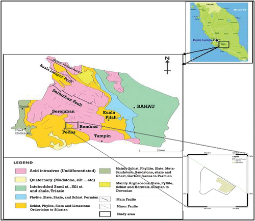
Pedas is a small district located in Negeri Sembilan. The research area is in the vicinity of the Seremban Fault Zone that lies within the West Belt Granite intrusion (Figure 1). The Seremban Fault Zone is recently recognised by curvilinear NW-SE trending faults, south of the Kuala Lumpur Fault Zone. The NW-SE faults are commonly associated with large quartz reefs, especially in the Pedas area Hutchison and Tan (2010). Meanwhile, Khalid and Derksen (1971), reported that the faults in Seremban are commonly associated with large quartz and pegmatitic dikes; Mylonite, sheared granites, and wide breccia zones characterising the fault zone within the granites. The present study area is located between the boundary of the granite and metamorphosed rocks called Pilah Schist. This formation is predominantly of grey carbonaceous shale; siltstone, phyllite, and schist with minor beds of arenite; slate, limestone, and volcanic (Khoo 1972). Established by Hutchison and Tan, (2009), the Pilah Schist contains two serpentinite bodies; the largest, about 6 km², outcrops along the main road to Tampin, 8 km south of Kuala Pilah.

Figure 1. Simplified geology of Negeri Sembilan (After Arisona et al. 2017) and the layout of the site (lower right).

3. Methodology

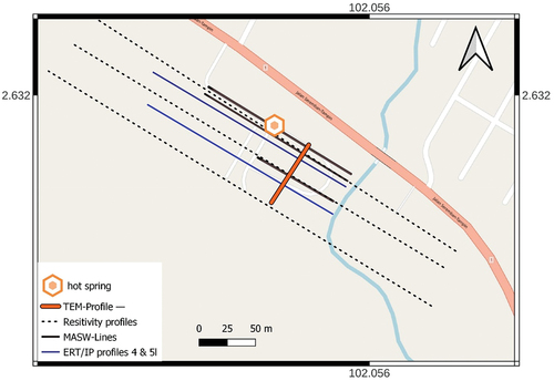
The field layout of the geophysical methods applied is presented in Figure 2. The distribution and length of profiles are controlled by the buildings inside the Wet World Complex. Three parallel ERT and MASW profiles trending NW-SE along with five TEM points trending NE-SE were conducted. The methodology of each geophysical method is presented in the following subsections.

Figure 2. Location map of geophysical field layout adopted in the present work.

3.1. Transient electromagnetic technique (TEM)

TEM is one of the surface geophysical methods that are used extensively to explore the size and vulnerability of aquifers. The method is used by many researchers for the characterisation of groundwater aquifers (e.g. Fitterman and Stewart 1986; Danielsen et al. 2003; Jørgensen et al. 2003; Khalil et al., 2016; Younis et al. 2016, 2019; Abdel Zaher et al. 2021). TEM simply adopts Faraday’s law in which a constant current is injected into the transmitter coil. This current produces a primary magnetic field. The current is then instantaneously switched off, according to Faraday’s law, the magnitude-changing primary field propagates in the subsurface. When it arrives at a conductive layer, an eddy current is generated. Such a current produces a secondary magnetic field that produces an electric current in the receiver coil at the surface. The magnitude and distribution of the electric current depend on the resistivity of the layer in which the eddy current was generated. Hence, the voltage measured at the receiver coil will correspond to the resistivity of that layer. As time lapses, the current penetrates deeper, producing a secondary magnetic field of deeper layers that produce voltages across the receiver coil. The recorded receiver voltage with time represents what is known as a decay curve that will be modelled to obtain the subsurface structures based on the resistivity parameter.

The present survey adopted a single-loop layout with a side length of 60 m. Such size can penetrate to a depth of about 180 m on average. The single loop acts as both the transmitter and receiver. TERRATEM instrument controls both transmitter and receiver in addition to sampling and recording of the data. Moreover, the instrument also provides basic processing tools that enable in-situ monitoring of the data quality average penetration depth.

The area surveyed with the TERRATEM instrument is about 60 × 100 m which accommodated five overlapping loops at an interval of 10 m spanning the total Pedas hot spring area. The loop started adjacent to the hot spring well and moved in the southwestern direction towards the Pedas River.

3.2. Multi-channel analysis of surface waves (MASW)

Multi-channel Analysis of Surface Waves (MASW) is introduced three decades ago that can produce shear wave velocity models at shallow depths at a low cost. The technique uses instrumentation similar to the conventional seismic refraction counterpart. They differ mainly in the frequency content of the seismic signal. MASW targets the low frequencies of the Rayleigh or Love waves, therefore, a low-cut filter that is often used in refraction work must be disabled when applying MASW. Besides, the geophones adopted for MASW should be of low natural frequency, preferably 4.5 Hz. Generally, MASW is applied to delineate the shear wave velocity model of the soil. Hence, the technique can give information about soil conditions and classifications. A quality control test was conducted in the field to select the best array parameters. From the results of the test, the shot offset of 15 m was preferred to produce the best dispersion curve. The geophones were mounted on a land streamer at 1 m intervals.

Field data acquisition consisted of three parallel lines. For each line, the shot increment was put at 5 m. Consequently, the total number of shot points was about 50. The first line was parallel to the outside fence and passed through the hot spring well. The second line was parallel to the first line with a 7 m offset. On the other hand, the third line was shorter than the first two lines because of some impediments, and the pool area at about 20 m from the second line.

3.3. Earth resistivity tomography (ERT) and IP

The Electrical Resistivity Imaging System was primarily carried out with a multi-electrode ABEM SAS 4000 resistivity metre. The survey utilised forty-one electrodes laid out in a straight line at regular spacing. A computer-controlled system was applied to automatically select two active electrodes for each measurement, (Griffiths and Barker 1993). The pole-dipole array method was employed for the data collection using RES2DINV software (Loke et al. 2006; Abdullah et al. 2022), to produce the resistivity images for modelling and interpreting the results.

The electrical resistivity methods, in essence, models the resistivity distribution of the subsurface materials. Table 1 shows the resistivity and conductivity values of some of the typical rocks and soil materials, (Keller George and Frischknecht Frank 1996). Igneous and metamorphic rocks typically have high resistivity values. The resistivity of rocks depends on some factors, namely; fluid electrolyte, porosity, temperature, and rock matrix (Hersir and Árnason 2010, and Ussher et al. 2000).

Table 1. Resistivity values of some subsurface rocks and soil materials (after Keller George and Frischknecht Frank 1996).

Material	Resistivity (Ω-m)
Alluvium	10 to 100
Sand	60 to1000
Clay	1 to 100
Groundwater (fresh)	10 to 100
Granite	5000 to 1,000,000

Rocks containing clay minerals, such as sediments, may result in induced polarisation in the subsurface rocks. The presence of clayey particles usually possesses negative charges that attract the positive ions from the fluid contents. In general, saltwater prevents the accumulation of particles and thus prevents the occurrence of induced polarisation, because the conductivity of saltwater is high, (Ayolabi et al. 2008). Accordingly, the IP model can differentiate between water-saturated aquifers and clay contents of soil or rocks.

IP measurements can be executed by either using direct current or alternating current. In this study, the direct current method was used. If measurements are made using direct current, the magnitude of the induced polarisation could be calculated as;

(1) $V_t/V_0$(1)

where V_t is the voltage after a time interval of t, and V₀ is the voltage during the current supplied. Table 2 shows the chargeability for some of the earth materials, modified after Murali and Patangay (2006).

Table 2. Earth materials and chargeability properties (modified after Murali and Patangay (2006).

Earth material	Chargeability (ms)
Water	0
Alluvium	1–4
Gravel	3–9
Sandstone	3–12
Quartzite	5–12
Schist	5–20
Argillites	5–10
Precambrian gneisses	6–30

4. Results and discussion

4.1. Multi-channel analysis of surface waves (MASW)

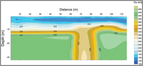
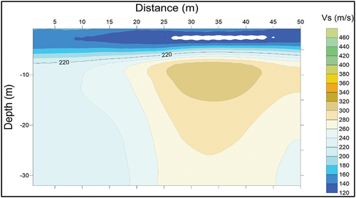
The inverted shear velocity model of line 1 (Figure 3) shows at a depth of 5 m, the velocity is below or equal to 180 m/s. This velocity is related to soft soil materials. At depths of between about 5 m and relatively 12 m, stiff soil materials were delineated. Depths delineated beyond this value were interpreted with velocities larger than 360 m/s. Near the centre of this line, low shear velocity values were observed to depths of about 40 m. This feature occurs adjacent to the hot water well location. The shear wave velocity anomaly could correspond to the fractures that control the flow of hot water to the surface in the Pedas area.

Figure 3. Shear wave velocity inversion of line 1 in the study area.

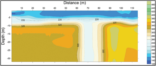
In line 2, (Figure 4), the same situation as in line 1 is observed, except for the stiff soil materials deepening to about 40 m towards the southeastern part of the profile. Adjacent to the hot water well site, an anomaly like that delineated in line 1 was observed. Nevertheless, the shear wave velocity values here are lower and the space distribution is wider.

Figure 4. Shear wave velocity model of line 2 in the study area.

Figure 5 is the inverted model for line 3, with the section showing only soil materials that range from soft to stiff. Hereby the soil section is increasing in the southwestern direction.

Figure 5. Shear wave velocity model of line 3 in the study area.

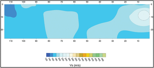
Furthermore, three depth slices were contoured at depths of 5, 18.5, and 32 m respectively. These slices demonstrate the distribution of shear wave velocities at these depths in the Pedas area. For the 5 m slice, (Figure 6), the soil is mostly made up of soft materials with shear wave velocity below 220 m/s.

Figure 6. Shear wave velocity depth slice at 5m in the study area.

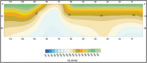
For the other two slices, (Figures 7 and 8), a real distribution show that the area near the outer fence is rocky with depths. By moving in the southwestern directions, stiff and soft soil materials were delineated. This could be due to the severe fracturing present in the area. It was also worthy of recognition adjacent to the hot water well in the southwestern directions, that low shear wave velocity was delineated in the form of a V shape having its head towards the well, then widening southwestward.

Figure 7. Shear wave velocity depth slice at 18.5m in the study area.

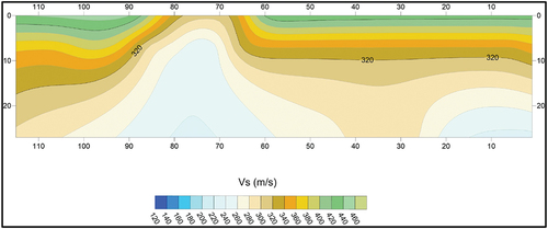
Figure 8. Shear wave velocity depth slice at 32.5m in the study area.

4.2. Earth resistivity tomography (ERT)

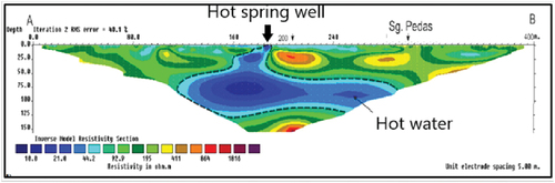
Three parallel ERT profiles were conducted within the premises of the Wet World Complex (Figure 2). The first profile was set up near the Hot Spring location and runs almost NW – SE directions. The profile length of the survey was set to 400 m with an electrode spacing of 5 m. The survey line crossed the main entrance road and the Pedas River in the Southeastern direction.

The inversion of the profile shows that adjacent to the hot spring well is characterised by low resistivity of 44 Ω.m represented by the blue colour zone (Figure 9). The zone reaches about 125 m in depth and dips in the SE direction. It is believed that this represents the near-surface accumulation of the hot water. The Pedas River (Sg. Pedas) runs close to the hot water accumulation and may be considered the main source of recharge to the hot spring.

Figure 9. 2D resistivity image inverted from the profile 1 data inverted by the RES2DINV program.

The inversion results for Profile 2 are shown in Figure 10. The model shows the hot water accumulation zone widens and extends to NW in addition to the SW extension in Profile 1. The movement of the hot water to the surface through the hot spring well is observed.

Figure 10. 2D resistivity image inverted from the profile 2 data inverted by the RES2DINV program.

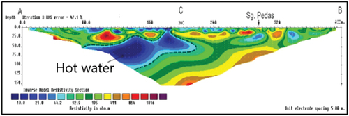
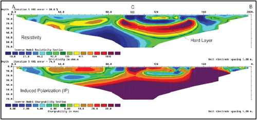
The resistivity model of the third parallel profile is shown in Figure 11. The profile has the same dimension and electrode spacings as the previous two profiles. Due to the present condition of the complex, part of this profile (the northwestern part) was conducted inside the main building of the complex. The model shows that the hot water accumulation zone becomes deeper. This indicates that the hot water zone dips in the SW direction. The dimension of the zone becomes smaller indicating cutting through harder rock.

Figure 11. 2D resistivity image inverted from the profile 3 data inverted by the RES2DINV program.

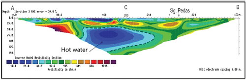
Figure 12. Fence diagram for ERT profiles 1 to 3 in the study area.

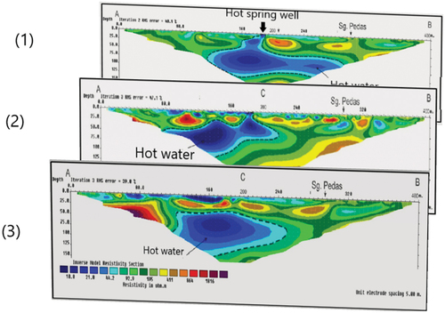
The fence diagram summarises the surveyed profiles 1 to 3 as presented in Figure 11. The figure gives a clearer image of the hot water reservoir and its position within the subsurface of the study area. From the illustration, we deduced that the hot water reservoir’s position matches the existing location of the hot spring well as observed from the surface and extended beyond about 40 m in the region of the well. The fence diagram gives a better understanding of the hot water reservoir pattern in the Pedas area. The figure gives a clearer picture of the existence of interconnectivity between the hot water reservoir for the Washing Well and the Hot Water Pool.

To meet the objective of investigating the subsurface soil materials around the Pedas area for expansion and redevelopment, two shallow profiles (i.e. profiles 4 and 5) were conducted using both the electrical resistivity and Induced Polarization (IP) methods. The model of profile 4 (Figure 13) shows a shallow layer possibly saturated with water down to a depth of about 20 m. This layer agrees well with the shallow layer identified from MASW. Underneath this layer, a relatively hard rock that possibly acts as cap rock is present until the end depth of the profile (i.e. depth = 60 m). The situation remains the same for profile 5 (Figure 14) with the surface layer seeming less saturated. This is indicated by the low resistivity and high chargeability. An interpretation of this situation could be the leakage from the hot water in the vicinity of the hot water well. The present study suggests that this leakage is due to the intersection of two faults there.

Both profiles 4 and 5 delineated subsurface hard layers, most probably a metasediment bedrock, in the study area at depths of between about 10 m to 30 m on these survey lines. The induced polarisation method showed a clearer pattern of subsurface hard layer structures, (e.g. the bedrock), distinctively than the resistivity method. This could be a result of the complexity involved in metasediment rocks. For redevelopment work, we suggested excavation at 10 m or preferably piling at deeper depths.

Figure 13. 2D resistivity (above) and chargeability (below) inversion models of the ERT/IP profile 4.

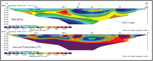
Figure 14. 2D resistivity (above) and chargeability (below) inversion models of the ERT/IP profile 5.

4.3. TEM model

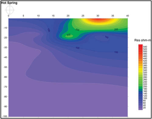
Five TEM survey points were conducted at the site starting from the northeast near the tar road and ending to the southwest at Pedas River. The target depth was about 180 m, however, because of the high noise at the site the maximum depth obtained was about 100 m. The trend of the TEM profile is perpendicular to the previous surveys in the present study. In Figure 15, the resistivity underneath the present hot spring is generally low corresponding to saturated soil. Moving away from the hot spring, the resistivity increases until the depth of 70 m. Below 70 m, the low resistivity prevails with no change throughout the profile. The highest resistivity corresponds to the shallow depth close to the Pedas riverbank. These features fairly agree with the ERT and IP models of profiles 4 and 5 in Figures 12 and 13, respectively.

Figure 15. TEM resistivity model in the vicinity of Pedas hot spring.

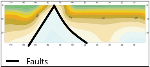
Also, Figure 16 illustrates the possible two faults according to the geophysical measurements carried out in the area of investigation at Pedas hot spring.

Figure 16. Possible two faults according to geophysical measurements of Pedas hot spring.

5. Conclusion

Four geophysical surveying techniques were utilised to suggest suitable locations for developing the recreational complex without affecting the hot spring flow. The methods adopted are MASW, ERT, IP, and TEM. ERT and TEM model the electric resistivity of the soil rocks. IP, on the other hand, models the electric chargeability that can help differentiate between water aquifers and other rocks that possess low resistivity. Besides, MASW models the shear wave velocity that is directly related to the soil strength. The model parameters obtained show low resistivity and low shear velocity anomalies underneath the hot spring. The anomaly is extending on both sides of the hot spring trending in the NE-SW direction. TEM showed that the low resistivity is deepening to a depth of 70 m close to the Pedas riverbank. IP models from profiles 4 and 5 agree with the TEM results with the possibility that the low resistivity anomaly below 70 m belongs to Schist or Phyllite with relatively high chargeability.

The output from all models suggests that the zone trending NE-SW may be considered as the shear zone controlling the flow of hot water to the surface. Building in this zone may have negative impacts on the hot spring. Besides, the information from the MASW modelling suggests that the northeastern boundary, excluding the low resistivity-shear velocity anomaly, is a suitable site for the complex structure extension.

Acknowledgments

The authors are grateful to those who assisted in the fieldwork during the data collection and analysis. Besides, Messrs Hariri Mohd Arifin and John Stephen Kayode thanked the University Sains Malaysia, and IPS for the Postgraduate and fellowship grants towards their doctoral research work respectively.

Disclosure statement

No potential conflict of interest was reported by the authors.

Correction Statement

This article has been corrected with minor changes. These changes do not impact the academic content of the article.

References

- Abdel Zaher M, Younis A, Shaaban H, Mohamaden MII. 2021. Integration of geophysical methods for groundwater exploration: a case study of El Sheikh Marzouq area, Farafra Oasis, Egypt. Egypt J Aquat Res. 47(2):239–244. doi:10.1016/j.ejar.2021.03.001.
- Abdullah FM, Loke MH, Nawawi M, Abdullah K, Younis A, Arisona A. 2022. Utilizing NWCR optimized arrays for 2D ERT survey to identify subsurface structures at Penang Island, Malaysia. J Appl Geophys. 196:104518. doi:10.1016/j.jappgeo.2021.104518.
- Abu-Hassanein ZS, Benson CH, Blotz LR. 1996. Electrical resistivity of compacted clays. J Geotech Eng. 122:397–406. doi:10.1061/(ASCE)0733-9410(1996)122:5(397).
- Archie GE. 1942. The electrical resistivity log as an aid in determining some reservoir characteristics. Trans AIME. 146(01):54–62. doi:10.2118/942054-G.
- Arisona A, Nawawi M, Khalil AE, Nuraddeen UK. 2017. Evaluation study of boundary and depth of the soil structure for geotechnical site investigation using MASW. Journal of Geoscience, Engineering, Environment.
- Árnason K, Eysteinsson H, Hersir GP. 2010. Joint 1D inversion of TEM and MT data and 3D inversion of MT data in the Hengill area, SW Iceland. Geothermics. 39(1):13–34.
- Ayolabi EA, Folorunso AF, Ariyo SO. 2008. Resistivity imaging survey for water supply tube wells in a basement complex: a Case Study of OOU Main Campus, Ago – Iwoye, South-western Nigeria. Proceedings of international Symposium on Hydrogeology of Volcanic Rocks (SHID): Republic of Djibouti. 67–71.
- Baioumy H, Nawawi M, Wagner K, Arifin MH. 2015. Geochemistry and geothermometry of non-volcanic hot springs in West Malaysia. J Volcanol Geotherm Res. 290:12–22. doi:10.1016/j.jvolgeores.2014.11.014.
- Danielsen JE, Auken E, Jørgensen F, Søndergaard V, Sørensen KI. 2003. The application of the transient electromagnetic method in hydrogeophysical surveys. J Appl Geophys. 53(4):181–198. doi:10.1016/j.jappgeo.2003.08.004.
- Fitterman DV, Stewart MT. 1986. Transient electromagnetic sounding for groundwater. Geophysics. 51(4):995–1005. doi:10.1190/1.1442158.
- Giao P, Chung S, Kim D, Tanaka H. 2003. Electric imaging and laboratory resistivity testing for geotechnical investigation of Pusan clay deposits. J Appl Geophys. 52(4):157–175.
- Griffiths D, Barker R. 1993. Two-dimensional resistivity imaging and modelling in areas of complex geology. J Appl Geophys. 29(3):211–226. doi:10.1016/0926-9851(93)90005-J.
- Hutchison, CS, Tan, DNK. 2009. Geology of peninsular malaysia. Geological Society of Malaysia and The Universiti of Malaya. 479.
- Hutchison, Tan D. 2010. GEOLOGY of PENINSULAR MALAYSIA 107p. published jointly by. The University of Malaya and The Geological Society of Malaysia.
- Jørgensen F, Sandersen PB, Auken E. 2003. Imaging buried Quaternary valleys using the transient electromagnetic method. J Appl Geophys. 53(4):199–213. doi:10.1016/j.jappgeo.2003.08.016.
- Keller George V, Frischknecht Frank C. 1996. Electrical methods in geophysical prospecting:11–23.
- Khalid BN, Derksen SJ. 1971. Geology of Eastern half of sheet 103. Ann. Report Geological Survey Malaysia. File Report. Min. Agriculture and Land, Gov Printing Office, Kuching.
- Khalil AE, Hafiez AH. 2016. The efficiency of horizontal to vertical spectral ratio technique for buried monuments delineation (case study, Saqqara (Zoser) pyramid, Egypt. 9:7.
- Khoo KK. 1972. Geology of Bahau area. Sheet 1o4 (Kuala Pilah) Negri Sembilan. Ann Rep Geol Survey Malaysia. 93–103.
- Loke M, Chambers J, Ogilvy R. 2006. Inversion of 2D spectral induced polarization imaging data. Geophys Prospect. 54:287–301. doi:10.1111/j.1365-2478.2006.00537.x.
- McCarter W. 1984. The electrical resistivity characteristics of compacted clays. Geotechnique. 34:263–267. doi:10.1680/geot.1984.34.2.263.
- Murali S, Patangay N. 2006. Principles and application of groundwater geophysics. 3rd ed. Hyderabad: Association of Exploration Geophysicists.
- Samsudin AR, Hamzah U, Rahman RA, Siwar C, Jani MFM, Othman R. 1997. Thermal springs of Malaysia and their potential development. J Asian Earth Sci. 15(2):275–284. doi:10.1016/S1367-9120(97)00012-6.
- Sum CW, Irawan S, Fathaddin MT. 2010. Hot springs in the Malay Peninsula. Proceedings World Geothermal Congress. Bali, Indon.
- Ussher G, Harvey C, Johnstone R, Anderson E. 2000. Understanding the resistivities observed in geothermal systems. Proceedings World Geothermal Congress 2000 Kyushu -Tohoku, Japan, May 28 June 10
- Younis A, Osman MO, Khalil A, Nawawia M, Soliman M, Tarabees A. 2019. Assessment groundwater occurrences using VES/TEM techniques at North Galala plateau, NW Gulf of Suez. Null. 160C(2019):103613. doi:10.1016/j.jafrearsci.2019.103613.
- Younis A, Soliman M, Moussa S, Massoud M, Abd El Nabi S, Attia M. 2016. Integrated geophysical application to investigate groundwater potentiality of the shallow Nubian aquifer at northern Kharga, Western Desert. Egypt NRIAG J Astron Geophys. 5:186–197.