Using microgravity techniques in the archaeology case study, the animal cemetery at Saqqara, Egypt

ABSTRACT

The use of microgravity technique for the detection of subsurface features is considered a valuable tool in archaeological prospection. The precise and detailed measurements obtained through this method have been crucial for the identification of buried structures. In the animal cemetery of Saqqara, a microgravity survey was conducted using a high-precision relative gravity metre called CG-5 device. This instrument has a standard resolution of 1 microGal (1 microGal = 10⁻⁸ m s⁻²) and a standard deviation of less than 5 microGals. The survey covered the entire animal cemetery, including the Ebbs tunnels, and was processed to calculate the vertical deviations in the area after applying terrain correction (TC). By detecting and delineating local density variations caused by a near-surface void, the microgravity technique was able to identify the presence of a possible void feature, as indicated by the acquired negative anomaly in the residual Bouguer anomalies. The precise gravitation data obtained after correction revealed that both the entrance of the cemetery and the densities of the burial chamber were relatively smaller than the surrounding areas of the animal cemetery in the Saqqara region. The data also showed the presence of two crypts leading to the burial chamber region in the southeast part of the cemetery. However, these preliminary results require further investigation, and the study area needs to be expanded to include a larger area. Additionally, other geophysical methods may be used to confirm the abnormality detected and verify the existence of a burial chamber or other corridors.

KEYWORDS:

• Saqqara
• the animal cemetery
• microgravity
• residual and bouguer anomalies
• archaeo-prospecting
• cavity detection

1. Introduction

Saqqara is a modern Egyptian village that lies on the western bank of the Nile, about 20 km southwest of Cairo, on the same limestone plateau that extends north to Giza. It is situated on the edge of the great Sahara Desert, and its cliff rises about 30 m above the valley. Saqqara is one of Egypt’s most important and richest necropolises, serving as the principal necropolis for the ancient capital Memphis. It has a long and extensive history, being used as a royal metropolis as early as the first and second dynasties, and as a burial place for supreme royal officials and dignitaries, as well as the Apis bulls, sacred to the principal deity during the Eighteen and Nineteenth dynasties of the New Kingdom.

The animal cemetery in Saqqara is a vast grid beneath the sands, crowded with remnants of millions of mummified animals, including dogs, cats, jackals, ducks, fish, and monkeys. The underground animal cemetery consists of a long central corridor and several smaller corridors branching off of it. A comprehensive map of the Saqqara region has been created, showing all the archaeological and exploratory mission sites active in the area (Figure 1). This map provides a simplified explanation of each archaeological landmark and each expedition in the Saqqara area, making it essential information for any visitor.

Figure 1. Detailed map of Saqqara including surveying area.

(Southern Jubban known as the animal cemetery).

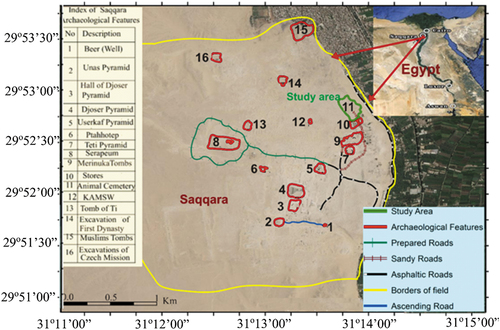
Several researchers have studied the geology of the Saqqara region, including Hume (1911), Blanckenhorn (1921, 1930), Youssef et al. (1984), and Papa (2003). According to Youssef et al. (1984), the Saqqara necropolis is situated on a plateau 17 metres above the Nile Valley’s alluvial plain (Figure 2), consisting mainly of Upper Eocene limestones, marls, and claystone. The southern cemetery of Saqqara is known as the animal cemetery, especially the Ibs tunnels, where thousands of cats and dogs were found, often mummified as pets or sacred animals.

Figure 2. Geologic map of Saqqara (Youssef et al. 1984).

Gravity is a widely used geophysical technique in engineering, environmental, and geological investigations, where geological boundaries, cavities, subsurface structures, subsoil anomalies, or landfills need to be detected. The microgravity method is a non-destructive detection method used in archaeological prospection (Linford 2006). Gravity observations are affected directly by density distribution under the surface, especially the existence of cavities creating a mass loss in proportion to the surrounding environment. In the microgravity method, a cavity or archaeological site produces a large density contrast (gravity lows) with negative amplitudes of several tens of microGals in the subsurface. This is very important in detecting hidden features on regional or large-scale gravity variations.

Cavities can be natural, such as solution cavities in limestone, or man-made, such as tunnels and archaeological sites, as noted by Bishop et al. (1997). It is not always the case that a negative anomaly is present; a positive anomaly may occur if a tomb has collapsed. To calculate height variance, the shift in gravity values at the same measurement points was combined with vertical changes in GNSS data, as demonstrated by Ergintav et al. (2007) and Bonforte et al. (2007). Given the limitations of the gravity method, including ambiguity stemming from the intrinsic nature of potential fields, it is necessary to use another geophysical technique to address such a complex environmental issue, as suggested by Hinze et al. (2013). This study relies on Ground Penetrating Radar (GPR) measurements taken in the same area, building upon the work of Mohamed et al. (2020).

2. Data acquisition

2.1. Microgravity data acquisition

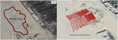
Microgravity data were collected using a Scintrex CG-5 gravimeter, which has an internal precision of ± 1 microGal. The data was acquired using regular and irregular grid systems, depending on the study (Figure 3). The grid spacing of measurement stations was determined based on the scale of the subsurface structures being delineated, and ranged from 1 to 1.5 metres.

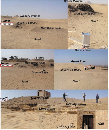
Figure 3. The area under study from all views.

To ensure the data quality, strict field procedures were followed. Accurate measurements were taken by measuring each point three times in a row for 60 seconds each time. The information was then saved on flash memory and could be sent to a printer, modem, recorder, or personal computer. Repeated tests were taken at stations with sudden shifts in gravity values to ensure accuracy.

During a single working day, approximately 100 to 150 points were observed. Figures 4 and 5 depict how the observations were collected. Figure 6 shows the distribution of monitoring points in the study area. The structural distance was very small, which guarantees the determination of geological structures of different sizes and depths.

Figure 4. The monitoring steps of the gravity and geodetic observations at the base station.

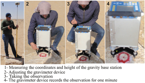
Figure 5. The research team accurately measures the gravity and position of the grid points.

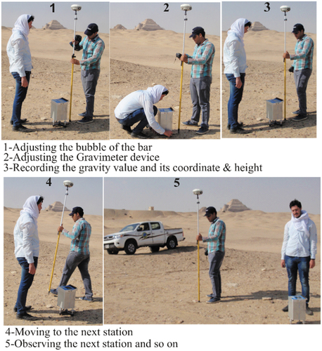
Figure 6. Distribution of the gravity and geodetic points in the southern Jubban area of Saqqara, Known as the animal cow.

2.2. Geodetic measurements

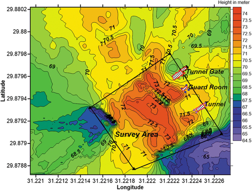
Geodetic measurements were conducted using an RTK-GNSS to determine the height of each microgravity station with a high accuracy of 1–2 cm. To ensure accuracy, five reference stations were established in the Saqqara area, as depicted in Figure 7, and a GNSS survey unit (base and rover) associated with the reference station was used. The Trimble R8 GNSS receiver was utilised for measurements, and the collected data was processed using Trimble software and adjustment programs (Trimble 2015). A 1-second sampling interval and 5° elevation mask angle were used during the field survey, with the calculation carried out using IGS precise ephemeris. After analysing the data and correcting various errors, high-resolution information within millimetres was obtained to serve ground gravity analyses in the Terrain correction calculation and provide accurate location information for mapping the workplace. Additionally, GNSS observations analysis enabled the creation of a topographic contour map with high accuracy, as depicted in Figure 8.

Figure 7. Installations of five GNSS reference stations in the Saqqara area.

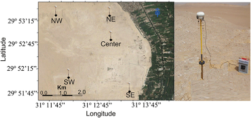
Figure 8. Topographic contour map of the study area.

2.3. Data processing and corrections

Ground gravity measurements are essential in geophysical surveys, but their accuracy can be affected by various factors such as the change in location, latitude, elevation, local terrain topography, earth tides, and rock densities. To improve the accuracy of these measurements, advanced survey methods are used to identify values at each point of observation. Corrections are then applied to the observations to account for various factors, including instrument drift, instrument response, earth tides, temperature changes, long-term drift, and other factors.

First, I want to clarify the concepts of ellipsoidal height and orthometric height and their relationship to GNSS technology and gravity reduction.

When using Global Navigation Satellite Systems (GNSS) technology, such as GPS, the height component provided is typically the ellipsoidal height. The ellipsoid is an idealised mathematical representation of the Earth’s shape, which is close to but not exactly the same as the geoid (the actual shape of the Earth’s surface, taking into account variations in gravity and irregularities).

Ellipsoidal height refers to the distance between a point on the Earth’s surface and the reference ellipsoid. It is calculated based on the position of the satellite and the receiver, taking into account the difference in their distances from the reference ellipsoid.

On the other hand, orthometric height, also known as the geodetic height or mean sea level height, refers to the vertical distance between a point on the Earth’s surface and the geoid (a hypothetical surface of equal gravity potential). It takes into account the variations in gravity caused by factors such as the Earth’s mass distribution and local topography.

Height correction is an important step to account for the effects of topography and terrain on gravity measurements. These corrections are necessary to accurately interpret gravity data and remove the influence of variations in elevation.

In our case, the height correction includes:

1. The free-air correction compensates for the change in gravity due to the elevation difference between the observation point and a reference height (usually sea level). It takes into account the decrease in gravitational acceleration with increasing height above the reference level. The free-air correction is typically applied as a linear correction based on the observed height and a constant gradient value.

2. The Bouguer correction accounts for both the free-air effect and the attraction of the mass between the observation point and the reference level. It considers the additional mass between the observation point and the reference level, such as the mass of the terrain. The Bouguer correction involves subtracting the calculated gravitational attraction of the additional mass from the observed gravity value. This correction is particularly important in regions with significant variations in topography.

3. The terrain correction aims to account for the gravitational effect of the local topography near the observation point. It considers the mass distribution within a certain radius around the observation point and calculates the gravitational attraction of the terrain. The terrain correction is often performed using numerical or analytical methods, considering the elevation and slope of the terrain in the vicinity of the measurement location.

The corrections applied to the observations can be automatic or manual, depending on the type of instrument used. The corrections include free-air correction, Bouguer correction, and latitude correction, and they are essential for interpreting geological data. A Bouguer gravity anomaly map is used to display the residual anomalies caused by shallow anomalous masses, and geological knowledge is needed to interpret these anomalies.

A Bouguer gravity anomaly map typically includes superposed anomalies from several sources. Regional anomalies are long-wavelength anomalies caused by deep density contrasts that are critical for understanding the large-scale structure of the Earth’s crust. The residual anomalies (short-wavelength anomalies) are caused by shallow anomalous masses that could be useful for archaeological prospecting. For interpreting the residual anomalies, geological knowledge is needed. The regional-residual separation of Bouguer gravity anomalies is carried out in the contexts.

The assumed average surface rocks density of 2.67 g/cc was selected to calculate Bouguer gravity anomalies. This density corresponds to the values determined from the average density of the surrounding topography. The resulting Bouguer anomaly map created in Surfer using the minimum curvature grid option is shown in Figure 9. The Bouguer gravity anomaly at the measurement point P is calculated based on the following formula:

Figure 9. Bouguer anomaly map explains the subsurface structures through accurate gravitation data after correction and elevation height of the topographic area. Both the cemetery entrance and burial chamber have relatively smaller densities for the areas around the southern catacomb (the animal cemetery) area in Saqqara.

$\mathrm{B}\mathrm{A}\left(\mathrm{P}\right)=\mathrm{g}\left(\mathrm{P}\right)-\mathrm{g}\mathrm{n}\left(\mathrm{P}0\right)+0.3086\mathrm{h}\left(\mathrm{P}\right)-0.0419\rho \mathrm{h}\left(\mathrm{P}\ast \right)+\mathrm{T}\left(\mathrm{P}\right)$

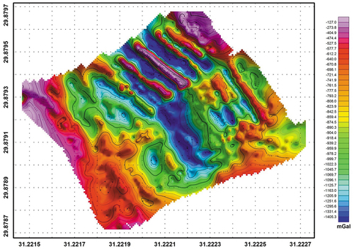
where g(P) is the measured gravity value (after drift and Earth tide corrections), gn(P₀) is the normal gravity field at the ellipsoid datum (P₀), −0.3086 h(P) is the free-air correction, +0.0419ρh(P_*) is the simple planar Bouguer correction, T(P) is the terrain correction, h(P) is the height of the gravity metre sensor position P, h(P_*) is the height of the point on the ground or floor, and ρ is the correction density.

• Drift and Tide Corrections

The time-dependent shifts in earth’s gravity, termed earth tides, are similar to the tidal changes of the earth’s oceans. Earth tides in any one location are cyclic in nature, oscillating between highs to lows diurnally and monthly. For instruments that do not have automatic drift corrections, the base measurements are used to remove both instrument drift and earth tide drift from the raw gravity data. To perform corrections, the raw gravity measurements for the base station are plotted on the y-axis against reading times on the x-axis, and a best fit curve or a series of line segments are fitted to the data. Other station measurements are then shifted up or down to intersect the drift curve based on the time each measurement was collected in relation to the base station measurements.

For instruments with auto-corrections, plotting base station measurements reveals the error associated with these corrections and allows for further refinement of the collected data. Theoretically, with auto-corrections, the repeat base station readings would be exactly the same value throughout the course of the survey.

For instrument drift, the automatic correction is determined prior to beginning a survey through repeated measurements at a specified test location for 24 hours. Automatic corrections for earth tides are performed similar to manual corrections using predictive earth tide charts, and when this feature is enabled, it is essential that the time, date, latitude, and longitude information is entered correctly into the gravimeter. If a base station is reoccupied throughout the day, additional drift corrections using the graphical method can be applied to compensate for any significant error remaining after applied auto-corrections.

The CG-5 manual recommends applying the instrument drift calibration once or twice a week for new instruments, decreasing to twice a month after the first four weeks. To ensure that drift corrections were accurate enough to avoid changing the instrument drift constant during consecutive days of data collection, the drift calibration were performed again during the 24 hours prior to beginning gravity survey. The data was plotted to verify its linear trend.

Once raw gravity readings collected in the field have been corrected for instrument drift and earth tide effects, the resultant data is termed observed gravity. All gravity reductions following drift corrections are applied using the following formula:

Observed Gravity – Theoretical Gravity = Gravity Anomaly

3. Results and interpretation of the microgravity data

The microgravity data was analysed using the Bouguer formula to determine the shift in ground gravity. The resulting Bouguer anomaly chart in Figure 9 showed several gravity lows and peaks, which were believed to be caused by deeper geological structures. To eliminate these anomalies, a planar regional trend was fitted to the gravity data and removed, resulting in a chart of residual gravity values. This regional-residual field separation was achieved using a low degree polynomial fitting method, as described by Linford (1998) and Padín et al. (2012).

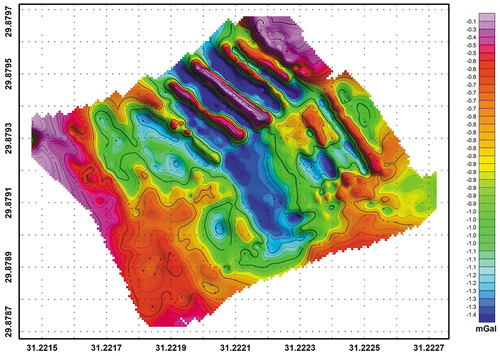
Figures 9–11 plotted the values of the change in ground gravity, which reflect the differences in the sub-surface density of the geological structures. This can provide valuable insights into unexplored cemeteries or burial chambers, including their location, distance, and depth. Through this analysis, the presence of two crypts leading to the burial chamber in the southeast part of the area was identified with greater accuracy.

Figure 10. Regional anomaly map shows an explanation of the subsurface structures through accurate gravitation data after removing the effect of the regional forces and after correction and elevation height of the topographic area.

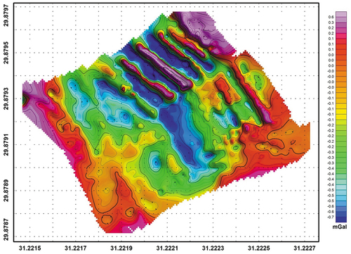
Figure 11. Residual anomaly map explains the subsurface structures through accurate gravitation data after removing the effect of any outside forces and after correction and elevation height of the topographic area.

In summary, the Bouguer formula was utilised to analyse microgravity data, and a regional-residual field separation method was employed to eliminate anomalies caused by deeper geological structures. This allowed for a more accurate identification of unexplored burial chambers, including the location, distance, and depth of these structures.

Based on the microgravity data and the Bouguer anomaly chart presented in Figures 9–11, it appears that there may be multiple subterranean chambers, cavities, corridors, and catacombs that were likely used for the burial of animals. However, further investigation is necessary to confirm these findings, such as expanding the study area to include a larger region and utilising additional geophysical methods to identify any anomalies that may indicate the presence of burial stones or other passageways.

4. Conclusions

Based on the results of the Microgravity study, it can be concluded that variations in ground gravity values are indicative of changes in sub-surface density of different geological structures, revealing the presence of unexplored cemeteries or burial chambers. In the southern catacomb (animal cemetery) area of Saqqara, subsurface structures’ density was relatively low. The figures and cross-sections presented in the study show the existence of multiple rooms, subsurface pits (cavities), corridors, and catacombs. The southeast part of the area contains two crypts leading to the burial chamber. However, further investigation is required to expand the study area and employ other geophysical methods to confirm the presence of any abnormality indicating the existence of a burial chamber or other corridors.

Acknowledgments

We gratefully acknowledge the financial support provided by project No.1348 from the Academy of Scientific Research and Technology. We would like to express our sincere thanks to the Geodynamics department’s workgroup at NRIAG for their valuable assistance in conducting the GPS and microgravity survey, particularly Dr. Mohamed Sobh, for his exceptional efforts. We also extend our appreciation to everyone who participated in the discussions and contributed to the successful completion of this work.

Disclosure statement

No potential conflict of interest was reported by the author(s).

References

- Bishop I, Styles P, Emsley SJ, Ferguson NS. 1997. The detection of cavities using the microgravity technique: case histories from mining and karstic environments. Mod Geophys Eng Geol, Geol Soc, Eng Geol Special Publication. 12(1):153–166. doi: 10.1144/GSL.ENG.1997.012.01.13.
- Blanckenhorn MP, (1921). Handbook of Regional Geologist, vol VII Dept. 9, Issue 23, Egypt: CarlWinters Universitatsbuch Dog Lung, Heidelberg, pp: 244.
- Bonforte A, Carbone D, Greco F, Palano M (2007). Intrusive mechanism of the 2002 NE-rift eruption at Mt Etna, Italy modelled using GPS and gravity data; Geophys J Int. 169 339–347.
- Ergintav S, Do˘gan U, Gerstenecker C, C¸akmak R, Belgen A, Demirel H, Aydın C, Reilinger R. 2007. A snapshot (2003–2005) of the 3D postseismic deformation for the 1999, Mw=7.4 İzmit earthquake in the Marmara Region, Turkey, by first results of joint gravity and GPS monitoring. J Geodesy. 44(1–2):1–18. doi: 10.1016/j.jog.2006.12.005.
- Hinze WJ, von Frese RRB, Saad AH. 2013. Gravity and magnetic exploration. principles, practices and applications. Cambridge: Cambridge University Press. doi: 10.1017/CBO9780511843129.
- Hume WF. 1911. The effect of secular oscillation in Egypt, during the Cretaceous and Eocene periods.Quart. QJGS. 67(1–4):118–148. doi: 10.1144/GSL.JGS.1911.067.01-04.05.
- Linford N. 2006. The application of geophysical methods to archaeological prospection. Rep Prog Phys. 69(7):2205–2257. doi: 10.1088/0034-4885/69/7/R04.
- Linford NT. 1998. Geophysical survey at Boden Vean, Cornwall, including an assessment of the microgravity technique for the location of suspected archaeological void features. Archaeometry. 40(1):187–216. doi: 10.1111/j.1475-4754.1998.tb00833.x.
- Mohamed A-MS, Atya M, AbouAly N, El Farragawy K, Hegazy EE, Saleh M, Kabeel K, ElMahdi AA. 2020. Mapping the archaeological relics of catacombs at Northeast Saqqara using GPR data, Egypt. NRIAG J Astron Geophys. 9(1):362–374. doi: 10.1080/20909977.2020.1746891.
- Padín J, Martín A, Anquela AB. 2012. Archaeological microgravimetric prospection inside don church (Valencia, Spain). J Archaeol Sci. 39(2):547–554. doi: 10.1016/j.jas.2011.10.012.
- Papa G, (2003). Site environmental analysis. The North Sakkara archaeological site: Handbook for the environmental risk analysis, Edizioni Plus, Universita Pisa. pp 180–203.
- Trimble NL. 2015. Geomatics software’s user manual. Sunnyvale, U.S.A: Trimble Navigation Limited.
- Youssef M, Cherif O, Boukhary M, Mohammed A. 1984. Geological studies on the Sakkara area. Egypt N Jb Geol Paläont Abh. 168(1):125–144. doi: 10.1127/njgpa/168/1984/125.