Evaluating the applicability of magnetic resonance sounding for groundwater exploration at selected locations in Aswan, Egypt

ABSTRACT

Magnetic resonance sounding (MRS) was performed to evaluate its applicability for characterising groundwater at selected locations in Aswan Governorate, Egypt. The MRS mainly detects a weak but noticeable alternating magnetic field as MRS signals when the proton spin in groundwater produces non-magnetic moments and rotates around the geomagnetic field, indicating the detection of groundwater. The MRS system was first correlated at a piezometer with a known water table depth (~80 m). Subsequently, three MRS sounding stations with unknown water tables were tested at Qism Aswan at ~ 18 km from the piezometer using NUMIS Auto magnetic resonance sounding system following the MRS site common practices. The MRS data were subjected to adaptive notch filtering to remove spiky noise and potential power line harmonics, and finally enhance the MRS signals at the selected stations. The water depth (~75–95 m) estimated from the MRS data around the piezometer largely coincides with the actual depth (~80 m) at the piezometer itself. A transient electromagnetic (TEM) profile performed near the measured MRS stations indicates no water content. Unlike the MRS data for NNL-1, the data for NNL-2 and NNL-3 match well with TEM data at shallow depths. The evaluation generally indicates that the MRS method is applicable for groundwater exploration at the selected piezometer and the other three stations. However, the method necessarily requires additional denoising efforts to comprehensively characterise groundwater occurrence and aquifer parameters.

KEYWORDS:

• Magnetic resonance sounding (MRS)
• piezometer
• groundwater
• Aswan

1. Introduction

The Magnetic Resonance Sounding (MRS) technique has demonstrated its effectiveness over recent years in various geological and geotechnical applications for groundwater investigations. The MRS can directly identify the presence of water by stimulating hydrogen protons within water molecules. Notably, MRS is the sole non-intrusive approach that examines groundwater reservoirs using surface measurements, primarily due to the direct connection between signal characteristics and aquifer properties (Lin et al. 2022). The inaugural use of MRS for exploring groundwater from the Earth’s surface was documented in the 1980s, as evidenced by Semenov (1987) and Legchenko et al. (1995). Extensive investigations and experimentation have been carried out across various geological contexts, specifically in sandy aquifers, clayey formations, fractured limestone, and in specialised test locations. These comprehensive studies have been reported by researchers such as Lieblich et al. (1994), Goldman et al. (1994), Legchenko et al (1995, 1997). Yaramanci et al. (1999), Meju et al. (2002), Plata and Rubio (2002), Lange et al. (2007), Vouillamoz et al. (2002), Yaramanci et al. (2002), and Baltassat et al. (2005).

The method’s ability to characterise groundwater aquifers without the need for drilling is attributed to its remarkable sensitivity to the presence of hydrogen protons in groundwater, as highlighted by Hertrich (2008), Vouillamoz et al. (2011), and Behroozmand et al. (2015). However, the relatively weak geomagnetic field intensity can result in the vulnerability of MRS signals to various forms of ambient noise, including spiky noise, power line harmonic noise, and random noise, as discussed by Levitt (2002) and Wang et al. (2018).

Nonetheless, the inversion processes applied to MRS signals offer valuable insights into the water content, pore properties, and subsurface conductivity of the aquifer, as demonstrated by research from Lachassagne et al. (2005) and Lubczynski and Roy (2005). Recent years have witnessed the development of innovative approaches for signal extraction to enhance precision, exemplified by the work of Ghanati et al (2014, Ghanati et al. 2016). Liu et al (2018, 2019). Over time, a variety of analytical techniques have been devised to mitigate noise interference, resulting in the establishment of a standardised MRS processing workflow, as reported in the studies by Legchenko and Valla (2003), Behroozmand et al. (2015), Jiang et al. (2011), Dalgaard et al. (2012), Costabel and Mueller-Petke (2014), Larsen et al. (2014), Larsen (2016), Walsh (2008), Dalgaard et al. (2012), Legchenko and Valla (2002), Strehl (2006), Lin et al. (2018), and Lin et al. (2019).

The primary premise of the MRS method involves the activation of Hydrogen atoms within water molecules through pulses of alternating current at the appropriate frequency (known as the Larmor frequency), which is sent into a loop positioned on the ground. The reactivity of H protons is contingent upon the strength of the Earth’s magnetic field, whereas the level of excitation affects the depth of groundwater. The magnitude of the magnetic field produced in response to the water in a layer is directly proportional to the porosity of the layer, and the time constant of the relaxation curve is closely associated with its permeability. The magnetic field is thereafter measured and scrutinised for different energising pulse magnitudes (intensity x time).

The primary utilisation of the MRS technique is to ascertain the water table at depths ranging from 100 to 150 m, enabling the identification of the optimal location for well drilling. The MRS has the capability to identify conductive faults within fractured aquifers and can provide recommendations for the optimal configuration of aquifer layers for hydrogeological modelling. The Prodiviner program is utilised for the procurement of Numis Poly data. The Samovar and Samogon software are utilised for the purpose of analysing and deciphering data to ascertain the depth of the water table, as well as the porosity and permeability of the distinctive aquifer. The benefits of the MRS approach in groundwater studies, compared to other geophysical methods, were demonstrated through a collection of field examples obtained from different countries such as Africa, Asia, Europe, and the US. These examples were cited in the works of Legchenko et al. (2006), Walsh (2008), and Qin et al. (2017), indicating the effectiveness and suitability of the MRS method. The MRS method has been utilised in hydrological research, permafrost thaw observation, glacier cavity monitoring, water-induced disaster detection, and infiltrating water surveys (Valois et al. 2018; Parsekian et al. 2019; Garambois et al. 2016; Shang et al. 2018; Falzone and Keating 2016).

An important limitation of using surface MRS for groundwater investigations is the existence of ambient noise (Hertrich, 2008), which impacts the accuracy of MRS measurements and renders them impractical in several situations. The signal received is notably feeble and susceptible to deterioration in the presence of ambient electromagnetic interference (Ghanati et al. 2016). Noise suppression remains a significant challenge in MRS data processing due to interference from noise. Extensive research has been conducted in the past few decades to develop denoising algorithms (Yao et al. 2019).

The MRS has some limitations in areas where sources of noises from nearby industrial areas are exist. For example, if magnetic rocks are dominant in the concerned area, they will induce a non-homogenous Earth’s magnetic field which makes difficulties to obtain a signal due to shift of frequency. In addition, sources of noise like power lines, pumps, industrial activity, buried pipes, fences, cyclic solar activity, magnetic storms … etc. can also induce some difficulties to obtain a good signal to noise ratio and so, consequently, an incapacity to measure a signal coming from the water subsurface protons. Noise can be considered as strong in MRS if it induces a voltage greater than 1–10 microvolts in a loop of 100 × 100 m, which approximately corresponds to a magnetic field of 0.01–0.1 milligammas.

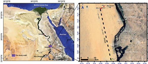
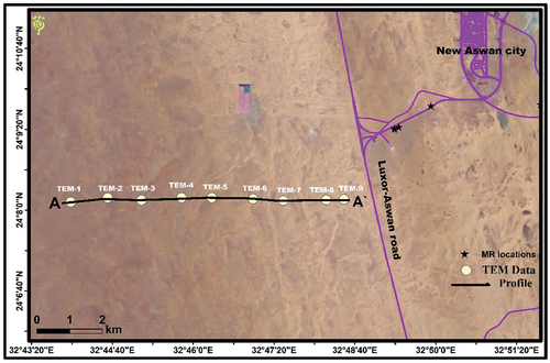
The study area is situated near Aswan, which is in the southern region of Egypt (Figure 1) and characterised by very high temperatures comparing to other Egyptian cities. Four MR sounding stations have been measured at Qism Aswan, Aswan Governorate, Egypt using NUMIS Auto magnetic resonance sounding system to evaluate the applicability of the MRS method for groundwater detection at shallow depth (~100 m). One station was used for calibration at a piezometer location where the water table was recorded at ~80 m depth. Three other MRS stations were measured ~18 km from the calibrated station following common practices for MRS site measurements. The aim of this research is to evaluate the possibility of applying magnetic resonance sounding (MRS) to explore groundwater at three selected sites in a seasonally hot climate area in Aswan.

Figure 1. Location map of MRS stations at Aswan Governorate, Egypt.

2. Geologic setting

The general geologic setting in the study area (Figure 2) and its vicinities has been studied by many authors such as Said (1990); Zaghloul et al. (1983); Hewaidy and Soliman (1993); Issawi and Osman (1996); Issawi et al. (2009), El Bastawesy et al. (2010) and Yousif (2019).

Figure 2. Geological map of the study area at Aswan Governorate, Egypt (CONOCO 1987).

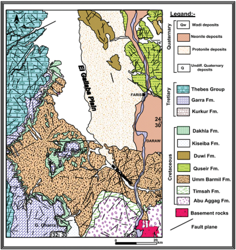
The Pre-Cambrian to Quaternary ages is represented in the region’s stratigraphic succession, which stretches from Aswan to the El Gallaba plain. Igneous and metamorphic rocks make up the majority of the Pre-Cambrian rocks. There is no ground surface exposure of the igneous rocks when travelling a short distance north of Aswan city. The age of the sedimentary layer that covers the basement complex varies from Paleozoic to Recent.

Based on the geologic map of Egypt (Luxor sheet, CONOCO 1987) (Figure 2) and Yousif (2019), the rock units in the study area are arranged in the following sequence, from bottom to top:

Upper Cretaceous Epoch: This epoch is characterised by the presence of several geological formations:

• Abu Aggag Formation, also known as the Nubian sandstone, represents the oldest sedimentary rock unit in the area. It predominantly comprises coarse sandstone with intermittent mudstone layers.

• Timsah Formation, another Nubian sandstone formation, is composed of siltstone, sandstone, and shales, with an iron ore bed. This formation can be observed to the southeast of the study area.

• Um Barmil Formation, also part of the Nubian sandstone, consists of medium sandstone with claystone layers. It spans the region to the south of Wadi El-Kubbaniya and the surrounding Gebel El Barqa area.

• Quseir Formation: is characterised by varicoloured shale, siltstone, and sandstone. It is exposed on the western side of the river Nile in the eastern part of El Gallaba Plain. The exposed section of this formation, found at Fares village, is approximately 40 m thick.

• Duwi Formation: is primarily composed of glauconitic sandstone with grey shale. It surfaces in the northeastern part of El Gallaba Plain, forming an elongated hill running from northwest to southeast with a thickness of about 15 m.

• Keseiba Formation: consists of fine-grained sandstone with shale and silt intercalations.

Tertiary Period: This period is represented by the following geological formations in the study area:

• Dakhla Formation (Paleocene-Eocene) is comprised of laminated varicoloured shale, typically ranging from grey to green, with occasional limestone layers. It is visible in the southwestern parts of Gebel El Barqa and in the southern region of Sin El Kaddab plateau. The shale in this formation has a thickness varying from 100 m to 135 m.

• Kurkur Formation (Paleocene) consists mainly of marly limestone, sandstone, and shale, along with thin layers of conglomerates and dolomitic limestone on top. This formation is situated along the eastern edge of Sin El Kaddab Plateau and in Gebel El Barqa, with an approximate thickness of 58 m.

• Garra Formation (Paleocene) unconformably overlies the Kurkur Formation and is primarily composed of limestone, some of which is chalky, with intercalations of marl and shale at the base. This formation can be found at the southeastern edge of Sin El Kaddab Plateau and in Gebel El Barqa, with an average thickness ranging from 15 to 20 m.

• Thebes group (Lower Eocene) is characterised by earthy brown limestone transitioning into greyish white limestone with chert. It is exposed in Gebel El Barqa and the northern part of Sin El Kaddab Plateau, with a thickness of approximately 200 m.

Quaternary Period: This represents the most recent deposits in the study area, covering most of the surface of El Gallaba Plain. These deposits primarily consist of alluvial sediments, which are a mixture of gravels, sands, silts, and mud.

3. Methodology

Magnetic resonance signals (MRS) occur when the spin of a proton in groundwater produces nonmagnetic moments and revolves around the geomagnetic field. When a weak magnetic moment is stimulated by an oscillating electromagnetic field at a particular frequency, the net magnetic moment will rotate by a specific angle away from the orientation of the Earth’s magnetic field. Upon the removal of the externally applied electromagnetic field, the overall magnetic alignment gradually returns to its initial condition, resulting in the production of a weak but noticeable alternating magnetic field at a larger scale. This magnetic field can be detected as a magnetic resonance sounding (MRS) signal in the receiving coil. The majority of research that interpret MRS data for petroleum and environmental applications typically analyse a single exponential decay that oscillates at the Larmor frequency, which is considered the MRS signal (Legchenko et al. 2002; Behroozmand et al. 2015).

Since the MRS methodology relies on energising and sending pulses of alternating current at a specific Larmor frequency to stimulate hydrogen atoms in water molecules, the resulting signal from the groundwater’s hydrogen protons is both excited and measured within the same loop (see Figure 3). To achieve accurate data, various pulse moments (measured in A.ms) are transferred into the loop, each corresponding to distinct depths of investigation. This process enables the determination of soil water content as a percentage (%) and is associated with the average pore size, which influences permeability.

Figure 3. MRS Methodology (Vermeersch 2000).

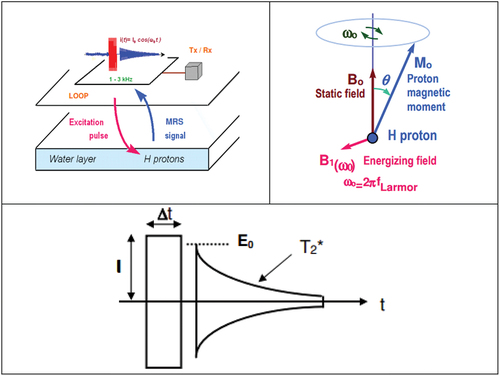
The static field B₀ (Earth’s magnetic field) determines the Larmor frequency of the H protons as follows:

Resonance Frequency f₀ (Hz) = 0.04258 × Earth magnetic field B₀ (nT)

The resonance frequency f₀ can provide the water content and the aquifer permeability in conjunction with the initial amplitude as follows: e(t) = E₀ exp (-t/T₂*) Sin (2π f₀ t + ф₀): relaxation with precession

E₀ =∑ (excitation field (1A) × (water content) × Sin (excitation field × duration)

Permeability = coefficient × water content × (time constant)²

Where E₀: Initial amplitude of signal (nV) proportional to the water content (%)

T₂*: Decay time constant of signal (ms) related to the pore size (permeability)

Δt: Excitation pulse moment (A.ms) related to the investigation depth (m)

Note that T₁ time constant gives better estimates of the permeability than T₂*. In general, T1 is < T2, but at low static field strength, as given in Earth’s field applications, they can be assumed to be equal. The MRS transverses the time constant (T2*) for estimation of the permeability. The dynamic energising field B₁ (loop magnetic field) produces the nutation of the H protons magnetic moment M₀: it tilts away from the static field with an angle θ, while still processing at the Larmor frequency. Once the energising field has been switched off, the protons come back to equilibrium (M₀ aligned with B₀) after a relaxation decay characterised by an initial amplitude E₀ and a time constant T₂*. The water content (porosity) is proportional to the amplitude of the proton response. The pore size of the medium (which is linked to the permeability) determines the time constant of this decay response. The depth of investigation is determined by the moment of the energising pulse (intensity x duration).

According to the MRS theory, the depth at which a measurement can be conducted changes depending on the moment of the excitation pulse. This moment is determined by multiplying the intensity of the current at the resonance frequency by the duration of the pulse. Consequently, it is feasible to assess the subsurface by employing MRS surface data. Furthermore, it can be demonstrated that the decay time constant of the relaxation field is correlated with the size of the pores, thus potentially enabling differentiation between pore-free water and clay bound water. In order to interpret an MRS sounding, it is necessary to assume that the subsurface is stratified on the same scale as the dimensions of the loop. The inversion procedure yields values for the water content, estimates of permeability, and the depth of each layer, obtained from the raw data for the entire set of pulse moments. To invert a collection of field data, the first step is to calculate a matrix that represents the expected response of thin water layers at different depths. This matrix considers the overall arrangement of the measurements, including the loop dimension, Earth’s field inclination, and ground resistivity. The calculation of this matrix typically requires approximately one hour on a personal computer, but the outcomes will be applicable to all the measurements conducted in a certain survey. The inversion process for a single set of data can be completed within a few seconds, allowing for prompt availability of results in the field before relocating the equipment to the next site. The inversion technique is completely automated, eliminating the need for an initial model.

To properly acquire the MRS data, three main functions of the acquisition software (i.e. Prodiviner) should be applied as follows:

1. Configuration

2. Test

3. Acquisition

Initially, we configure the settings by specifying the necessary parameters for input into the software to initiate data acquisition. This includes defining the loop type, dimensions, and the Earth’s magnetic field value for the particular area. Advanced settings such as stacking, pulse parameters, and pulse moments are typically left at default values for standard configurations. The subsequent step involves testing the system’s tuning and assessing the ambient noise level before commencing the measurement.

Upon completing the initial steps, an estimated acquisition time is provided at the start of the sounding. To initiate the acquisition, the process is triggered by clicking the “Start” button in the status bar. This action opens the “Signal” window, displaying continuous measurement of the current pulse moment, including the MRS signal and noise in the “Positive signal envelope” section. The graph updates after each stack and with each new pulse moment, presenting data in terms of signal amplitude (in nV) versus time (in ms).

Following each measurement, corresponding to the maximum number of stacks for each pulse moment, the upper-left graphic in the “Sounding” section is updated. Here, data is presented in relation to the maximum MRS signal amplitude (in nV) and the time constant (T2*) value, displayed in relation to pulse moments (A.ms).

Upon completing the full sounding, data is imported into the provided interpretation software for further analysis.

4. MRS data acquisition

The MRS data was collected using the NUMIS poly MRS system (NUMIS 1996; Vermeersch 2000) (Figure 4) at four locations in Aswan Governorate, three at Qism Aswan, and one near Aswan University (Table 1). The MRS system used for data acquisition consists of several units as shown in Figure 4(4) and is used mainly for the direct detection of shallow groundwater. It is a modular multi-channel MRS equipment designed with units weighting 25 kg or less. The MRS system has one converter, which is sufficient to investigate the existence of groundwater at 100 m depth using a 100 m side-square loop (400 m total length). Before collecting the MRS data, the average value of the Earth’s magnetic field should be measured at several points inside the loop area to define the transmitter frequency, and thus we can configure the capacitors.

Figure 4. NUMIS poly multi-channel magnetic resonance sounding system.

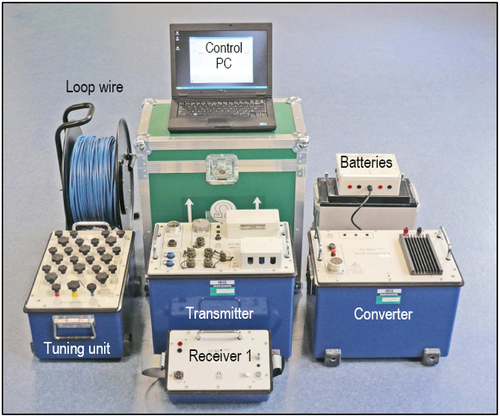
Table 1. Locations of MR stations, Aswan (December, 3–10, 2021).

Sr.	MR Station	Coordinates	Location	Site Photo
1	Piezo-1	23°59’41.4“N 32°51’10.2“E	Near Aswan University, Aswan Governorate
2	NNL-1	24°09’43.0“N 32°49’55.4“E	Qism Aswan, Aswan Governorate
3	NNL-2	24°09’20.4“N 32°49’19.0“E	Qism Aswan, Aswan Governorate
4	NNL-3	24°09’22.3“N 32°49’23.4“E	Qism Aswan, Aswan Governorate

The Geometrics G-856 type Overhauser magnetometer was used to determine the mean magnitude of the Earth’s magnetic field. Multiple measurements were conducted at intervals of 10 m along two intersecting lines within the loop to verify the consistency of the magnetic field and to produce a dependable mean value. The amplitude’s lateral variation should not exceed ±20 nT for accurate measurements, which is approximately equivalent to ±1 Hz.

When we started the data acquisition, the geomagnetic field value was entered in the “Field” area of the “Configuration” window of the data acquisition software (i.e. Prodiviner of IRIS). The acquired raw data will be stored in a binary file (”. Pro” extension), and then read/save in “txt” by this program.

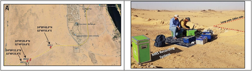
The MRS data was first acquired at one station (called Piezo-1) located at ~ 8 metres from the piezometer location near Aswan University, Aswan Governorate, Egypt (Figure 5). For further evaluation of the MRS survey at Aswan area, three locations were selected (Figure 6) and measured by the NUMIS system. They are named NNL-1, NNL-2 and NNL-2. The NNL-1 is about 1 km from NNL-2, and the NNL-2 is about 0.15 km from NNL-3. The average value of the geomagnetic field was 41,103.9 (nT), while the Larmor frequency was 1750.1 hertz (Hz). Both the transmitter and receiving coils had dimensions of 100 m × 100 m and consisted of one-turn square coil. The coils were arranged in a coincident loop arrangement.

Figure 5. Location of the MRS station at a piezometer (left) with a known water table (~80m depth) near Aswan University, Aswan Governorate, Egypt. The calibrated piezometer (right) is located at ~8 meters from the measured MRS station.

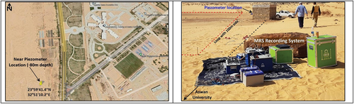
Figure 6. Location of three MRS stations (left) at ~18 km from a known piezometer near Aswan University, Aswan, Egypt. MRS survey at NNL-1 station (right), Qism Aswan, Aswan, Egypt.

The raw data was preprocessed using statistical stacking and adaptive notch filtering to remove spiky noise and potential power line harmonics. Next, stacking was used 16 times at each pulse moment to improve the Signal to Noise Ratio (SNR). Figure 7 shows a screen shot of the operation display (upper photo) of the Prodiviner software during the acquisition process at Piezo MRS station where the following parameters were set up to start the data acquisition:

Figure 7. The selected and resultant data acquisition parameters in the Prodiviner software.

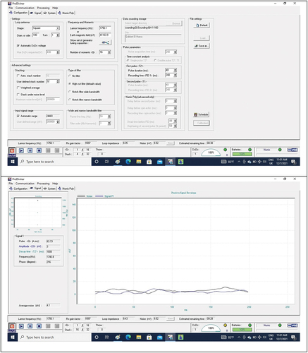
• Shape of the loop antenna: square

• Diameter or side of the loop: 100 m

• Larmor frequency (Hz): 1750.1

• Average value of the Earth’s magnetic field (nT): 41103.9

• Number of moments (Q): 16

• Stack was set to: 32

Meanwhile, the lower photo indicates the resultant parameters based on the above selection in the upper photos:

• Pulse (Q) (A.ms): 83.73

• Amplitude (EQ) (nV): 3

• Decay time (T₂) (ms): 1000

• Frequency (Hz): 1740.8

• Phase (degree): 216

• Average noise (nV): 4.1

The MRS equipment is used to detect groundwater on-site. The signal received by the receiver coils consists of both the MRS signal and electromagnetic noise. The emission current induces the movement of hydrogen protons in groundwater towards elevated energy levels. Following the removal of the emission current, hydrogen protons undergo lateral relaxation and decay, resulting in the emission of electromagnetic waves with the Larmor frequency, which propagate outward (Yao et al. 2019). Subsequently, the receiving coil captures the electromagnetic waves that carry the MRS signal at the Larmor frequency. (Hertrich et al. 2007; Legchenko 2013)

5. MRS data analysis

5.1. MRS computation – matrix program

Before inverting the MRS data, it is necessary to compute a matrix. The Matrix computation program is installed, by default, in the “Program Files|Iris Instruments|Interpretation” directory. The “NUMIS Matrix” is representative of a geoelectrical model of the subsurface. The procedures for running the Matrix computation software are as follows:

• Define a 1-D geoelectrical section, if known, by selecting the number of layers and enter the estimated depth of each layer and their resistivity.

• Then press “Run” in the “File” area and enter the storage file name (“mrm” extension file) – A new file for each time should be created. The computation takes a few seconds. One matrix can be used for the interpretation of several MRS soundings as the local parameters do not usually change significantly in a given local survey area.

5.2. Samogon - modelling software

The Samogon program is installed, by default, in the “Program Files|Iris instruments|Tools” directory. The main functions of Samogon software can be described in two main steps:

• Configuration of the model.

• Creation and fitting of the model.

The model consists of a number of water-saturated layers in the subsurface defined by the matrix. For each layer, several parameters have to be defined. After having defined the layer’s parameters, we used the “Make” button of the “Make model” area to create the model and save it in a ”.mod” file. The graphic then shows the model curves and the RMS error will be displayed to visualise the fitting on that model with respect to the sounding data. It’s then possible to adjust the model to the sounding data by modifying one of the model parameters.

5.3. Samovar - inversion software

The Samovar is an automatic inversion software. The main functions of this automatic inversion can be described in two main steps:

• Configuration of the inversion parameters

• Inversion results

Meanwhile, the purpose of Samovar software is to know:

1. Water table depth

2. Water contents

3. Type of aquifer (shallow, deep) or multiple aquifer (shallow + deep)

The computation of the data matrix typically takes approximately one hour on a standard PC, but the results remain applicable for all soundings conducted in the same area. Subsequently, the actual inversion of a set of data is a rapid process, lasting only a few seconds. These results can be made available either on-site before relocating the equipment to the next site or later in a laboratory setting. The inversion procedure is entirely automated, eliminating the need for an initial model. However, the operator does have the option to manually adjust the regularisation parameter’s value to either smooth or accentuate variations in water content with depth, based on the specific local conditions or equivalence properties. Following the validation of inversion parameters, the program proceeds with the inversion process and verifies the coherence between the matrix used and the data file to prevent any errors. Subsequently, the “Data windows” appear, displaying various parameters. The primary parameters of the software in use are presented in the following manner (refer to Figures 8, 9 , 10 , and 11)

Figure 8. MRS Results at Piezo-1 around the existing piezometer, Aswan Governorate, Egypt.

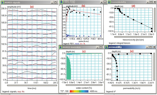
Figure 9. MRS Results at NNL-1, Qism Aswan, Aswan Governorate, Egypt.

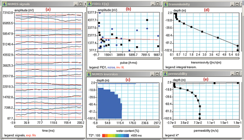
Figure 10. MRS Results at NNL-2, Qism Aswan, Aswan Governorate, Egypt.

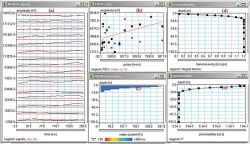
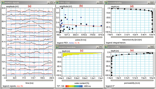
Figure 11. MRS Results at NNL-3, Qism Aswan, Aswan Governorate, Egypt.

1. Relaxation curves of MRS signal and an exponential fit versus time. NUMIS Signals window.

2. Max. measured amplitude of the signal versus the pulse moment: FID1: E(q) window.

3. Numis inversion result (water content versus depth): NUMIS Inversion window.

4. Frequency versus pulse moment: FID1: Freq(q) window.

5. Decay time versus pulse moment: FID1: T₂*(q) window.

6. Phase versus pulse moment: FID1: Phase (q) window.

7. If T1 has been measured: decay time versus pulse moment: T₁(q) window.

8. Permeability value versus depth (Permeability) window.

6. MRS data interpretation

MRS analysis allows for the estimation of water depth, water content, and mean pore size (permeability) of individual layers at specific depths. These parameters are valuable for assessing the potential of a groundwater reservoir prior to drilling. In order to understand an MRS sounding, it is necessary to assume that the subsurface is stratified on a scale that matches the dimensions of the loop, such as 100 m in this particular study. The inversion procedure yields values for water content, estimates of permeability, and the depth of each layer, obtained by analysing the raw data for the entire set of pulse moments. In order to invert a collection of field data, the initial step is to calculate a matrix that represents the expected response of thin water layers situated at different depths. This matrix considers the overall arrangement of the measurements, including the loop dimension, inclination of Earth’s magnetic field, and ground resistivity.

In a general sense, the interpretation of MRS data provides the following outputs:

• Signal relaxation curves (in nV) plotted against time (in ms) for different injected pulse moments, with the smallest values at the bottom and the highest at the top. These signals are depicted in black, while the expected 1D fits are shown in red.

• Sounding curve: This represents the initial amplitude (in nV) of the signal relaxation curves for each pulse moment value (in A.ms). Raw data points are marked in black, noise in blue, and the red curve corresponds to the theoretical model response determined through inversion.

• Inversion result: This provides the water content (porosity) represented as a percentage versus depth in metres. The colour-coding of sectors is indicative of the time constant of layer permeability, measured in metres per second (m/s), as a function of depth in metres.

The value of the permeability is estimated through the following relation:

Permeability = Cp_x × Porosity × (T₁)2;

Cp_x is a coefficient, which can be modified in the configuration window, after calibration with the results of pumping tests.

According to the MRS theory, the depth at which a measurement can investigate varies depending on the moment of the excitation pulse. This moment is determined by multiplying the intensity of the current at the resonance frequency by the duration of the pulse. Consequently, MRS surface measurements can be used to probe the ground. Furthermore, it has been demonstrated that the decay time constant of the relaxation field is correlated with the size of the pores, which has the ability to differentiate between pore-free water and clay-bound water (Bernard 2004). The results of the MRS test (Figure 8) at the piezometer location show NUMIS signals (Figure 8a) that reflects the relationship between the amplitude (nV) and the time (ms). The MRS data indicate interesting results because the signal is well represented above the noise level (Figure 8b) and indicates good quality data. The presence of a water layer is represented in the inversion at a deeper depth (~75-95 m), and it is also visible in the data at high moment. (Figure 8c) indicates variable results of water content with depth, for example, at high values of T₁ (e.g. ~300–400 ms), the water content is high and vice versa. Transmissivity (Figure 8d) describes the ability for fluid flow within the plane of the material and is defined as the in-plane permeability multiplied by the material thickness. The transmissivity of the piezometer increases due to the increase of the permeability with depth (Figure 8d). The permeability (K) versus depth curve (Figure 8e) indicates the increase of K near the ground surface from ~2.5 m to ~10 m, and gradually decreases from ~10 m to ~22 m, and then gets stable from ~22 m to ~102 m.

The results of the MRS test (Figure 9) at station NNL-1 shows the signal relaxation curves (nv) versus time (ms) for varying pulse moments (Figure 9a). The MRS results indicate relatively noisy data with a noise level up to ~ 3500 nanoV (Figure 9b).

This noise level was not expected because the MRS test was carried out in a relatively open desert area with no apparent source of noise. We expect that this noisy data is caused by unseen sources (e.g. abandoned pipes or rubbish metal materials) that definitely affect the quality of the data. However, (Figure 9c) shows that the decay time T₂ represents unexpected values in such case (T₂ ≥500 ms), and indicates the presence of water content at variable depths ranging from ~18 m to ~100 m. The transmissivity shows increasing values with depths from ~ 10 to 100 m (Figure 9d). The resulting permeability (K) (Figure 9e), the ability of a material to allow fluids (typically water) to pass through it, shows high values near the ground surface and decreases from ~5 m to ~20 m depth, and then increases from ~20 m to ~70 m, and then becomes constant from ~70 m to ~100 m. This geologically indicates that the Nubian sandstone (intercalations of sand and clay) which is dominant in the study area has variable stratigraphic textures that show fluctuations of the permeability values with depth. In other words, high permeability near the ground surface indicates geological strata that are likely consist of porous materials such as loose sediments (e.g. sand or gravel). Meanwhile, low permeability (~5 m to ~20 m depth) indicates a transition to denser less porous materials such as compacted sediments or less fractured rock formations. Increase in permeability again from ~20 m to ~70 m depth may suggest the presence of more porous lithologies as loose sand. Stability of the permeability values from ~70 m to ~100 m depth could indicate the presence of relatively homogeneous stratigraphic materials with consistent permeability properties within this depth range. It is also possible that these deeper layers consist of more compacted or less fractured rock formations, resulting in constant permeability values as clay or shale.

The results of the MRS test (Figure 10) at station NNL-2 shows the signal relaxation curves (nv) versus time (ms) for varying pulse moments (Figure 10a). Similarly, the MRS results of station NNL-1 indicate relatively noisy data with a noise level up to ~ 8000 nanoV (Figure 10b). This noise level was not expected because the MRS test was carried out in a relatively open desert area that do not clearly contain any surface source of noise. We expect that this noisy data is caused by unseen sources (e.g. abandoned pipes or rubbish metal materials) that definitely affect the quality of the data. However, Figure (10c) shows that the decay time T₂ represents unexpected values in such a case (T₂ ≥500 ms), and indicates the presence of water content at high moments at very shallow depths ranging from the ~1 m to ~15 m. The transmissivity (Figure 10d) increases from the ground surface to ~20 m and gets stable from ~20 m to ~100 m depth. The resulting permeability (K) (Figure 10e) shows high values near the ground surface and decreases from ~5 m to ~18 m depth, and then becomes constant from ~18 m to ~100 m. This geologically indicates that the Nubian sandstone (intercalations of sand and clay) which is dominant in the study area has variable stratigraphic textures that show fluctuations of the permeability values with depth. In other words, high permeability near the ground surface indicates geological strata that are likely consist of porous materials such as loose sediments (e.g. sand or gravel). Meanwhile, low permeability (~5 m to ~18 m depth) indicates a transition to denser less porous materials such as compacted sediments or less fractured rock formations. Stability of the permeability values from ~18 m to ~100 m depth could indicate the presence of relatively homogeneous stratigraphic materials with consistent permeability properties within this depth range. It is also possible that these deeper layers consist of more compacted or less fractured rock formations, resulting in constant permeability values as clay or shale.

The results of the MRS test (Figure 11) at station NNL-3 shows the signal relaxation curves (nv) versus time (ms) for varying pulse moments (Figure 11a). The MRS data shows relatively good results because the pulse moment amplitude signal is well represented above the noise level (Figure 12b) and indicates good quality data. However, the presence of the water layer is not represented in the inversion curve (Figure 11c) of the water content versus depth where T₂ (≤300 ms). The transmissivity (Figure 11d) increases from ~1 m to ~15 m, and decreases steadily with depths from ~15 m to ~100 m.

Figure 12. Location of TEM profile, Qism Aswan, Aswan Governorate, Egypt (Khalifa 2023).

The resulting permeability (K) (Figure 11e) shows high values near the ground surface and decreases from ~10 m to ~15 m depth, and then becomes constant from ~15 m to ~100 m. This geologically indicates that the Nubian sandstone (intercalations of sand and clay) which is dominant in the study area has variable stratigraphic textures that show fluctuations of the permeability values with depth. In other words, high permeability near the ground surface indicates geological strata that are likely consist of porous materials such as loose sediments (e.g. sand or gravel). Meanwhile, low permeability (~10 m to ~15 m depth) indicates a transition to denser less porous materials such as compacted sediments or less fractured rock formations. Stability of the permeability values from ~15 m to ~100 m depth could indicate the presence of relatively homogeneous stratigraphic materials with consistent permeability properties within this depth range. It is also possible that these deeper layers consist of more compacted or less fractured rock formations, resulting in constant permeability values as clay or shale. The water content represents only a thin wet surface layer (Figure 11c) with low permeability and transmissivity.

7. Correlation of the MRS data with TEM data

The MRS results at the conducted four stations were correlated with one transient electromagnetic (TEM) profile located near the study area (Figure 12). The TEM profile (Khalifa 2023) was measured by AIE-2 variant equipment at 9 locations arranged in E-W direction using a single square loop configuration (Coincident loop). The TEM stations were performed with a single loop configuration, each loop is 25 m × 25 m (2500 m²) (Figure 12).

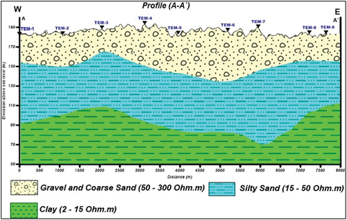
The processed TEM data of the 9 stations has been utilised to construct a geologic cross-section (Figure 13) to provide a tentative description of the subsurface geology in the study area. The interpreted geologic cross section of profile A-A′ refers to three geoelectric layers as shown in Figure 13(13).

1. The first surface layer: consists of alluvial deposits of gravels and coarse sand, and characterised by relatively high resistivity values ranging from 50Ω to 300Ω and a varying thickness ranging from ~40 m to 45 m. At TEM station-1, this layer is no longer present due to the occurrence of a fault.

2. The second layer: composed of silty sandstone, which is characterised by lower resistivity values ranging from 15Ω to 50Ω, and a varying thickness ranging from ~60 m to 80 m.

3. The third layer: primarily consists of clay, which exhibit very low resistivity values ranging from 2Ω to 15Ω. The thickness of this layer could not be determined in the current geoelectric survey as it extends beyond the depth that was explored.

Figure 13. Geologic cross-section A-A′ of the interpreted TEM profile.

Considering the MRS results near the TEM profile (A-A′), it has been noticed that the TEM data has not indicated the presence of water along the measured profile, which means that the groundwater reservoir is very low. However, to compare the TEM results with the MRS data, we analysed the most important parameters (i.e. transmissivity and permeability) that could be evidence of the presence of water in the studied locations. For example, the transmissivity, the rate at which water is transmitted through a unit width of an aquifer under a unit hydraulic gradient, at Piezo station (Figure 8d) increases with depth, however, the permeability (K) (Figure 8e) shows fluctuating values (K=~ −4.4 e⁻⁶ to ~ 2.0 e⁻⁵ m/s) from the ground surface up to ~22 m, and then gets stable from ~22 m to ~102 m (K = ~2.0 e⁻⁵ to ~ 2.7 e⁻⁵ m/s), indicating moderate to high water content ranges from ~ 75-95 m, which is in a good agreement with the actual water depth at the piezometer itself (~80 m). The transmissivity (Figure 9d) at NNL-1 station increases with depth, however, the resulting permeability (Figure 9e) shows fluctuated values from the ground surface up ~70 m (K=~ −3.7 e⁻³ to ~ 7.3 e⁻² m/s) and then becomes constant from ~70 m to ~100 m (K=~ 7.3 e⁻² m/s), indicating unexpected results where the water content shows moderate to high percentages. The resulting permeability (K) (Figure 9e) geologically indicates that the Nubian sandstone (intercalations of sand and clay) which is dominant in the study area has variable stratigraphic textures that show fluctuations of the permeability values from the ground surface to ~70 m depth indicating geological strata that are likely consist of moderately porous materials such as friable sediments (e.g. sand or gravel). Stability of the permeability values from ~70 m to ~100 m depth could indicate the presence of relatively homogeneous stratigraphic materials with consistent permeability properties within this depth range. It is also possible that these deeper layers consist of more compacted or less fractured rock formations, resulting in constant permeability values as clay or shale.

The transmissivity (Figures 10d & 11d) and the resulting permeability (Figures 10e & 11e) at stations NNL-2 and NNL-3 show variable results, indicating very low water content at shallow depth.

8. Conclusion

The magnetic resonance sounding (MRS) was experimentally implemented at four stations in Aswan Governorate, Egypt. It was a good approach to evaluate the applicability of the method in groundwater characterisation at the selected locations. The MRS method was first performed at a piezometer with a known water table depth (~80 m) to evaluate its applicability for detecting the groundwater parameters. This helped us to properly correlate the MRS results and proceed the measurements with the most appropriate parameters at three other selected locations with unknown water tables. The MRS measurements around the piezometer zone showed that the estimated water depth was ~ 75-95 m, which largely coincides with the actual depth (~80 m) at the piezometer itself. Meanwhile, the MRS results at NNL-1 station showed that the water content generally rises from a moderate to high level as the resulting decay time T₂ is ≥500 ms, and the estimated water depth is generally found to be from ~ 18 to ~100 m. The MRS results at stations NNL-2 and NNL-3 show variable results, indicating very low water content at shallow depth. On the other hand, the transient electromagnetic (TEM) profile performed near the measured MRS stations indicates the absence of water content. There is a clear match between the MRS data at stations NNL-2 and NNL-3 and the TEM data as both indicate the absence of water content.

Although the MRS data at stations NNL-1, NNL-2, and NNL-3 were likely affected by noises of unknown origin, the applied filter relatively enhanced the results that provided good information about the water table in the piezometer area, and reasonable information at the other three stations. It is worth noting that the issue of denoising the MRS data for signal enhancement is still under profound study around the world. Several groups worldwide are nowadays conducting intensive research in noisy environments to understand, describe and record surface MRS signals that may lead to further improvement of the MRS method. The evaluation generally indicates that the MRS method is applicable for groundwater exploration at the selected piezometer and the other three stations. However, the MRS method necessarily requires additional application with denoising software to comprehensively characterise groundwater occurrence and aquifer parameters.

Acknowledgments

The authors express gratitude for the assistance of the National Research Institute of Astronomy and Geophysics (NRIAG, Egypt) in supplying the NUMIS magnetic resonance instrument, the overhauser magnetometer, cars, and field assistants. The authors would also like to express their gratitude for the valuable time and effort devoted by the esteemed reviewers in reviewing the paper. They also appreciate the thorough and constructive comments provided by the reviewers.

Disclosure statement

No potential conflict of interest was reported by the author(s).

References

- Baltassat JM, Legchenko A, Ambroise B, Mathieu F, Lachassagne P, Wyns R, Mercier JL, Schott JJ. 2005. Magnetic resonance sounding (MRS) and resistivity characterization of a mountain hard rock aquifer: the Ringelbach Catchment, Vosges Massif, France. Near Surf Geophys. 3(4):267–274. doi: 10.3997/1873-0604.2005022.
- Behroozmand AA, Keating K, Auken E. 2015. A review of the principles and applications of the NMR technique for near-surface characterization, Surv. Surv Geophys. 36(1):27–85. doi: 10.1007/s10712-014-9304-0.
- Bernard J. 2004. MRS: step-by-step operation of NUMIS systems. Orléans, Cedex 2, France: IRIS Instruments.
- CONOCO. 1987. Geological map of Egypt. NG 36 SW LUXOR. Scale. 1:500000.
- Costabel S & Mueller-Petke M. 2014. Despiking of magnetic resonance signals in time and wavelet domain, Near Surf. Geophys. 12(2):185–198. doi: 10.3997/1873-0604.2013027.
- Dalgaard E, Auken E, Larsen JJ. 2012. Adaptive noise cancelling of multichannel magnetic resonance sounding signals. Geophys J Int. 191:88–100. doi: 10.1111/j.1365-246X.2012.05618.x.
- El Bastawesy M, Faid A, Gammal ESE. 2010. The Quaternary development of tributary channels to the Nile River at Kom Ombo area, Eastern Desert of Egypt, and their implication for groundwater resources. Hydrol Process. 24(13):1856–1865. doi: 10.1002/hyp.7623.
- Falzone S, Keating K. 2016. Algorithms for removing surface water signals from surface nuclear magnetic resonance infiltration surveys. Geophysics. 81(4):WB97–WB107. doi: 10.1190/geo2015-0386.1.
- Garambois S, Legchenko A, Vincent C, Thibert E. 2016. Ground-penetrating radar and surface nuclear magnetic resonance monitoring of an englacial water-filled cavity in the polythermal glacier of Tête Rousse. Geophysics. 81(1):WA131–WA146. doi: 10.1190/geo2015-0125.1.
- Ghanati R, Fallahsafari M, Hafizi MK. 2014. Joint application of a statistical optimization process and empirical mode decomposition to magnetic resonance sounding noise cancellation. J Appl Geophys. 111:110–120. doi: 10.1016/j.jappgeo.2014.09.023.
- Ghanati R, Hafizi MK, Fallahsafari M. 2016. Surface nuclear magnetic resonance signals recovery by integration of a non-linear decomposition method with statistical analysis. Geophys Prospect. 64:489–504. doi: 10.1111/1365-2478.12296.
- Goldman M, Rabinovich B, Rabinovich M, Gilad D, Gev I, Schirov M. 1994. Application of integrated NMR-TDEM method in ground water exploration in Israel: Jour. Appl Geophys. 31(1–4):27–52. doi: 10.1016/0926-9851(94)90045-0.
- Hertrich M. 2008. Imaging of groundwater with nuclear magnetic resonance, progress in nuclear magnetic resonance spectroscopy. Prog Nucl Magn Reson Spectrosc. 53(4):227–248. doi: 10.1016/j.pnmrs.2008.01.002.
- Hertrich M, Braun M, Gunther T, Green AG, Yaramanci U. 2007. Surface nuclear magnetic resonance tomography. IEEE Trans Geosci Remote Sens. 45:3752–3759. doi: 10.1109/TGRS.2007.903829.
- Hewaidy AA, Soliman SI. 1993. Stratigraphy and paleoecology of gabal elborga, south-west Kom Ombo, Nile Valley, Egypt. Egypt J Geol. 37:299–321.
- Issawi B, Francis M, Youssef A, Osman R. 2009. The Phanerozoic of Egypt: a geodynamic approach. 81:571. Ministry of Petroleum and the Egyptian Mineral Resources Authority Special Publication
- Issawi B, Osman R. 1996. The sandstone enigma of south Egypt. 3rd Conf Geology Of The Arab World Cairo Univ. 359–380.
- Jiang C, Lin J, Duan Q, Sun S, Tian B. 2011. Statistical stacking and adaptive notch filter to remove high level electromagnetic noise from MRS measurements. Near Surf Geophys. 9(5):459–468. doi: 10.3997/1873-0604.2011026.
- Khalifa M. 2023. Geophysical Studies to Determine the Subsurface Structures and Hazard Assessment of the Extensions of New Aswan City, Egypt. [ PhD. thesis Fac. Sci]. Aswan Univ. 317.
- Lachassagne P, Baltassat JM, Legchenko A, de Gramont HM. 2005. The links between MRS parameters and the hydrogeological parameters. Near Surf Geophys. 3(4):259–265. doi: 10.3997/1873-0604.2005021.
- Lange G, Yaramanci U, Meyer R. 2007. Surface nuclear magnetic resonance in environmental geology. Berlin: Springer.
- Larsen JJ. 2016. Model-based subtraction of spikes from surface nuclear magnetic resonance data. Geophysics. 81(4):WB1–WB8. doi: 10.1190/geo2015-0442.1.
- Larsen J, Dalgaard E, Auken E. 2014. Noise cancelling of MRS signals combining model-based removal of power line harmonics and multichannel Wiener filtering. Geophys J Int. 196:828–836. doi: 10.1093/gji/ggt422.
- Legchenko A. 2013. Magnetic Resonance Imaging for Groundwater. 1st ed. London: John Wiley & Sons, Inc; p. 131–132.
- Legchenko A, Baltassat JM, Martin C, Robain H, Vouillamoz JM. 2002. Magnetic resonance sounding applied to catchment study. Eegs. 41–44, Aveiro.
- Legchenko AV, Beauce A, Guillen A, Valla P, Bernard J. 1997. Natural variations in the magnetic resonance signal used in MRS groundwater prospecting from the surface. Eur J Environ Eng Geophys. 2:173–190.
- Legchenko A, Descloitres M, Bost A, Ruiz L, Reddy M, Girard JF, Sekhar M, Kumar MSM, Braun JJ. 2006. Resolution of MRS applied to the characterization of hard-rock aquifers. Groundwater. 44(4):547–554. doi: 10.1111/j.1745-6584.2006.00198.x.
- Legchenko A, Shushakov O, Perrin J, Portselan A. 1995. Noninvasive NMR study of subsurface aquifers in France. SEG Houston Conference abstract. Houston, USA. p. 365–367.
- Legchenko A, Valla P. 2002. A review of the basic principles for proton magnetic resonance sounding measurements. J Appl Geophys. 50(1–2):3–19. doi: 10.1016/s0926-9851(02)00127-1.
- Legchenko A, Valla P. 2003. Removal of power-line harmonics from proton magnetic resonance measurements. J Appl Geophys. 53(2–3):103–120. doi: 10.1016/s0926-9851(03)00041-7.
- Levitt MH. 2002. Spin Dynamics: basics of Nuclear Magnetic Resonance. London: John Wiley & Sons.
- Lieblich DA, Legchenko A, Haeni FP, Portselan A. 1994. Surface nuclear magnetic resonance experiments to detect subsurface water at Haddam Meadows, Connecticut. Proceedings of the Symposium on the Application of Geophysics to Engineering and Environmental Problems; [27–31 Mar 1994]; Boston, MA; 717–736, vol. 2.
- Lin T, Li Y, Lin Y, Chen J, Wan L. December 2022. Magnetic resonance sounding signal extraction using the shaping-regularized Prony method. Geophys J Int. 231(3):2127–2143. doi: 10.1093/gji/ggac317.
- Lin TT, Zhang Y, Mueller-Petke M. 2019. Random noise suppression of magnetic resonance sounding oscillating signal by combining empirical mode decomposition and time-frequency peak filtering. IEEE Access. 7(79):917926. doi: 10.1109/ACCESS.2019.2923689.
- Lin TT, Zhang Y, Yi XF, Fan TH, Wan L. 2018. Time–frequency peak filtering for random noise attenuation of magnetic resonance sounding signal. Geophys J Int. 213(2):727–738. doi: 10.1093/gji/ggy001.
- Liu L, Grombacher D, Auken E, Larsen JJ. 2018. Removal of Co-Frequency Power line Harmonics from Multichannel Surface NMR Data. IEEE Geosci Remote Sens Lett. 15(1):53–57. doi: 10.1109/LGRS.2017.2772790.
- Liu L, Grombacher D, Auken E, Larsen JJ. 2019. Complex envelope retrieval for surface nuclear magnetic resonance data using spectral analysis. Geophys J Int. 217:894–905. doi: 10.1093/gji/ggz068.
- Lubczynski M, Roy J. 2005. MRS contribution to hydrogeological system parametrization, Near Surf. Geophys. 3(3):131–139. doi: 10.3997/1873-0604.2005009.
- Meju MA, Denton P, Fenning P. 2002. Surface NMR sounding and inversion to detect groundwater in key aquifers in England: comparisons with VES–TEM methods. J Appl Geophys. 50(1–2):95–111. doi: 10.1016/S0926-9851(02)00132-5.
- NUMIS. 1996. Manual of NUMIS system for Proton Magnetic Resonance 56. Orléans, Cedex 2, France: IRIS Instruments.
- Parsekian AD, Creighton AL, Jones BM, Arp CD. 2019. Surface nuclear magnetic resonance observations of permafrost thaw below floating, bedfast and transitional ice lakes. Geophysics. 84(3):EN33–EN45. doi: 10.1190/geo2018-0563.1.
- Plata J, Rubio F. 2002. MRS experiments in a noisy area of a detrital aquifer in the south of Spain. J Appl Geophys. 50(1–2):83–94. doi: 10.1016/S0926-9851(02)00131-3.
- Qin S, Ma Z, Jiang C, Lin J, Xue Y, Shang X, Li Z. 2017. Response characteristics and experimental study of underground magnetic resonance sounding using a small-coil sensor. Sensors. 17(9):2127. Reconstruction. IEEE Trans. Image Process. 16,349–366, doi:10.1109/tip.2006.888330.
- Said R. 1990. The geology of Egypt. Amsterdam- (NY): Elsevier Publishing Co.
- Semenov AG. 1987. NMR Hydroscope for water prospecting. Proceedings of the Seminar on Geotomography, Indian Geophysical Union; Hyderabad; p. 66–67.
- Shang X, Jiang C, Ma Z, Qin S. 2018. Combined system of magnetic resonance sounding and time-domain electromagnetic method for water-induced disaster detection in tunnels. Sensors. 18(10):3508. doi: 10.3390/s18103508.
- Strehl S. 2006. Development of strategies for improved filtering and fitting of surface NMR signals. M.Sc thesis. Berlin University of Technology.
- Valois R, Vouillamoz JM, Lun S, Arnout L. 2018. Mapeamento de reservas de águas subterrâneas no noroeste do Camboja com uso combinado de dados litológicos e sondagens eletromagnéticas de domínio de tempo e por ressonância magnética. Hydrogeol J. 26(4):1187–1200. doi: 10.1007/s10040-018-1726-1.
- Vermeersch F. 2000. NUMIS Plus equipment operating manual. Orléans, Cedex 2, France: IRIS Instruments.
- Vouillamoz JM, Descloitres M, Bernard J, Fourcassier P, Romagny L. 2002. Application of integrated magnetic resonance sounding and resistivity methods for borehole implementation. A case study in Cambodia. J Appl Geophys. 50(1–2):67–68. doi: 10.1016/S0926-9851(02)00130-1.
- Vouillamoz JM, Legchenko A, Nandagiri L. 2011. Characterizing aquifers when using magnetic resonance sounding in a heterogeneous geomagnetic field. Near Surf Geophys. 9(2):135–144. doi: 10.3997/1873-0604.2010053.
- Walsh DO. 2008. Multi-channel surface NMR instrumentation and software for 1D/2D groundwater investigations. J Appl Geophys. 66:140–150. doi: 10.1016/j.jappgeo.2008.03.006.
- Wang Q, Jiang C, Mueller-Petke M. 2018. An alternative approach to handling co-frequency harmonics in surface nuclear magnetic resonance data. Geophys J Int. 215(3):1962–1973. doi: 10.1093/gji/ggy389.
- Yao X, Zhang J, Yu Z, Zhao F, Sun Y. 2019. Random noise suppression of magnetic resonance sounding data with intensive sampling sparse reconstruction and kernel regression estimation. Remote Sens. 11(15):1829. doi: 10.3390/rs11151829.
- Yaramanci U, Lange G, Hertrich M. 2002. Aquifer characterisation using surface NMR jointly with other geophysical techniques at the Nauen/Berlin test site. J Appl Geophys. 50(1–2):47–65. doi: 10.1016/S0926-9851(02)00129-5.
- Yaramanci U, Lange G, Knodel K. 1999. Surface NMR within a geophysical study of an aquifer at Haldensleben (Germany. Geophys Prospect. 47(6):923–943. doi: 10.1046/j.1365-2478.1999.00161.x.
- Yousif M. 2019. Hydrogeological inferences from remote sensing data and geoinformatic applications to assess the groundwater conditions. El-Kubbaniya basin, Western Desert, Egypt. J Afr Earth Sci. 152:197–214. doi: 10.1016/j.jafrearsci.2019.02.003.
- Zaghloul ZM, El-Shahat A, Ibrahim A. 1983. On the discovery of Paleozoic trace fossils. Bifungites in the Nubian Sandstone facies of Aswan area. Egypt J Geol. 27:25–72.