Contribution of geostatistics for the representation of the basement-sediment contact with gravity data

ABSTRACT

In this work, a fast method of representation of the basement-sediment contact in a sedimentary zone is presented. The proposed approach is based on the polygonal model and stacked rectangular prism model. This approach consists of separate the Bouguer anomaly into regional and residual ones by using the polynomial method to better locate the sediment deposits. Then, 2D gravity modelling of several profiles plotted on the residual anomaly map is done. The data collected from these models are interpolated by the geostatistical method of Kriging to obtain the model of the basement-sediment contact of the study area. The feasibility and reliability of the proposed approach are demonstrated on synthetic data produced by a prism, and satisfactory results have been obtained. The inversion of real gravity anomalies is presented as a practical example to get a better view of the basement-sediment contact of the transition zone between the Benue and Lake Chad basins. The obtained 2D and models show that the sediment deposits are mainly constituted of sandstones. The maximum depth of these sediments is 5.5 km around the locality of Lagdo. In addition, these sedimentary deposits are less deep and almost absent in the north of Garoua, Bibemi, Kaele and Maroua.

KEYWORDS:

• Geostatistic
• kriging
• 2D inversion
• basement-sediment

1. Introduction

Civil engineering works, in particular, the installation of large structures, the construction of large bridges (Danyang Kunshan bridge in China, Dardanelles Strait bridge in Turkiye) and the establishment of canals for the drainage of large quantities of water (Suez Canal in Egypt, Panama Canal in Central America), are fundamentally linked to the study of the basement (Giao et al. 2003; Sultan et al. 2007). Detailed knowledge of the structure and composition of the latter is therefore a prerequisite for the construction of these infrastructures under appropriate technical and financial conditions. The mapping of the basement-sediment contact has for some time been a great progress and success in the determination of the geometric parameters allowing the realisation of these infrastructures as well as in the search for buried ores and structures associated with oil or gas deposits (Chen et al. 2008; Hinze et al. 2013; Zhdanov 2015). The evaluation of the depth and extension of the sediments from this representation of the basement-sediment contact makes it easy, for example, to choose the drilling points (Witter et al. 2016). In recent years, several authors have developed and proposed methods, approaches, tools and computer codes to estimate the geometric parameters of anomaly sources. Notably, imaging methods for field data, numerical methods for forward modelling of potential fields (Zhao et al. 2018; Fadakinte 2022) and 3D Cauchy-type integrals (Cai and Zhdanov 2015a, 2015b; Nazanin et al. 2021) are significant. The practical application of these modelling methods requires a lot of computing time and storage space. Most of these approaches are presented in the form of computer codes and are generally integrated into software, which makes them difficult to use. To solve this problem, we propose in this work a new simple and fast method of representation of the basement-sediment contact thanks to the geostatistical method of kriging using gravimetric data. This method starts from the polynomial anomaly separation of Bouguer, then defines the 2D models thanks to the polygonal model of Talwani et al. (1959) and the stacked model of Bott (1960) and finally makes a statistical evaluation of the basement-sediment contact by the geostatistical method of kriging (Krige 1951) thanks to the data extracted from the 2D models. We check the fiability and efficiency of this method by testing it on synthetic data produced by a prism. After this test, we evaluate the basement-sediment contact of the transition zone between the Benue and Lake Chad basins.

2. Methods

2.1. Polynomial separation

In this work, we present a 3D representation method of the basement-sediment contact of a sedimentary zone. To do this, it is therefore necessary to have the expression of the residual anomaly which expresses the contribution of the superficial structures, hence the need for the separation of the Bouguer anomalies into regional and residual.

The regional Bouguer anomaly at a point $\left(x_i,y_i\right)$ can be represented by a polynomial function in the form of equation (1)(1) $\mathit{r}\left(x_i,y_i\right)=\sum _{\mathit{r}=0}^n\sum _{\mathit{s}=0}^n{c}_{\mathit{rs}}{x}^r{y}^s$(1) (Njandjock et al. 2012).

(1) $\mathit{r}\left(x_i,y_i\right)=\sum _{\mathit{r}=0}^n\sum _{\mathit{s}=0}^n{c}_{\mathit{rs}}{x}^r{y}^s$(1)

where, $\mathit{r}\left(x_i,y_i\right)$ is the regional value of the Bouguer anomaly at $\left(x_i,y_i\right)$; $\left(\mathit{n}\right)$ is the degree of the polynomial and $c_{\mathit{rs}}$ represents the polynomial coefficients. These coefficients are determined by the Gauss pivot method by minimising the quadratic deviation $\mathit{E}$ given by equation (2)(2) $\mathit{E}=\sum _{\mathit{i}=1}^N{\left[r\left(x_i,y_i\right)-\mathit{b}\left(x_i,y_i\right)\right]}^2$(2) in the least-squares sense according to equation (3)(3) $\frac{\mathrm{\partial E}}{\mathrm{\partial }{\mathit{C}}_{\mathit{rs}}}=0$(3) .

(2) $\mathit{E}=\sum _{\mathit{i}=1}^N{\left[r\left(x_i,y_i\right)-\mathit{b}\left(x_i,y_i\right)\right]}^2$(2)

(3) $\frac{\mathrm{\partial E}}{\mathrm{\partial }{\mathit{C}}_{\mathit{rs}}}=0$(3)

where, $\mathit{b}\left(x_i,y_i\right)$is the value of the Bouguer anomaly at the position $\left(x_i,y_i\right)$ and $\mathit{N}$ the number of stations where, the Bouguer anomaly is known. Then, we can thus deduce the residual anomaly at any point using equation (4)(4) $\mathit{r}{ }^{\mathrm{\prime }}\left(x_i,y_i\right)=\mathit{b}\left(x_i,y_i\right)-\mathit{r}\left(x_i,y_i\right)$(4) .

(4) $\mathit{r}{ }^{\mathrm{\prime }}\left(x_i,y_i\right)=\mathit{b}\left(x_i,y_i\right)-\mathit{r}\left(x_i,y_i\right)$(4)

A good separation requires a better choice of the degree of the polynomial representing the regional anomaly. To determine this degree, Zeng (1989) proposed a method that is a compromise between upward continuation and polynomial smoothing. This method consists of evaluating the height $\mathrm{h}$ beyond which the upward prolonged gravity anomalies remain similar in shape and change only in amplitude. A polynomial smoothing of degree $\mathrm{d}$varying from $1$ to $12$ is then applied to the anomalies resulting from the upward continuation at altitude $\mathrm{h}$. The appropriate degree of the regional polynomial is estimated from the point of discontinuity on the graph of the minimum variance ${\sigma }_d$ as a function of the degree of the polynomial. This minimal variance between the grid of $\mathrm{M}$ values of the prolonged Bouguer at altitude $\mathrm{h}$ noted $b_h\left(x_i,y_i\right)$ and that of the region for different degrees noted $r_d\left(x_i,y_i\right)$ is given by equation (5)(5) ${\sigma }_d=\frac{1}{M}\sum _{\mathit{i}=1}^M{\left[b\left(x_i,y_i\right)-r_d\left(x_i,y_i\right)\right]}^2$(5) :

(5) ${\sigma }_d=\frac{1}{M}\sum _{\mathit{i}=1}^M{\left[b\left(x_i,y_i\right)-r_d\left(x_i,y_i\right)\right]}^2$(5)

where,

(6) $\mathit{b}\left(x_i,y_i\right)=a_0+a_1{x}_i+a_2{y}_i+\dots +a_k{y_i}^{\mathit{n}}$(6)

(7) $r_d\left(x_i,y_i\right)=b_0+b_1{x}_i+b_2{y}_i+\dots +b_k{y_i}^{\mathit{d}}$(7)

(8) $\mathit{d}=1,2,\dots ,\mathit{n}-1,\mathit{n},\mathit{n}+1,\dots$(8)

A Matlab code taking into account the different equation (equation 1(1) $\mathit{r}\left(x_i,y_i\right)=\sum _{\mathit{r}=0}^n\sum _{\mathit{s}=0}^n{c}_{\mathit{rs}}{x}^r{y}^s$(1) , 2(2) $\mathit{E}=\sum _{\mathit{i}=1}^N{\left[r\left(x_i,y_i\right)-\mathit{b}\left(x_i,y_i\right)\right]}^2$(2) , 3(3) $\frac{\mathrm{\partial E}}{\mathrm{\partial }{\mathit{C}}_{\mathit{rs}}}=0$(3) , 4(4) $\mathit{r}{ }^{\mathrm{\prime }}\left(x_i,y_i\right)=\mathit{b}\left(x_i,y_i\right)-\mathit{r}\left(x_i,y_i\right)$(4) ) of this separation method has been set up (Nlen Wounle et al. 2023).

2.2. 2D gravity inversion

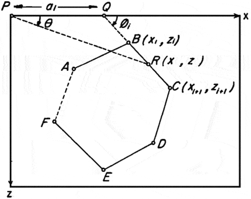
For a better representation of the basement-sediment contact, in a sedimentary zone, the 2D inversion is more important. The 2D gravity inversion method applied in this work consists of the decomposition of the initially preconceived structure into prisms of polygonal section and infinite elongation; the calculation of the effect of these prisms is then added. The anomaly is calculated by varying the physical parameters of the disturbing structure, in particular its shape, depth and density. The best model is that which corresponds to the structure whose calculated anomaly most closely approximated to the observed anomaly by adjustment. According to Talwani et al. (1959), if ABCDEF (Figure 1) is a given polygon with n-sides and P the point where the attraction due to this polygon is determined.

Figure 1. Geometry of elements involved in the gravitational attraction of an n-sided.

The expressions $\mathit{V}$ and $\mathit{H}$ are respectively the vertical and horizontal components of the field created by a body assimilated to this polygon. They are given by equation (9)(9) $\mathit{V}=\mathit{G}\underset{x}{\int }\underset{y}{\int }\underset{z}{\int }\Delta \mathit{\rho zdxdydz}{(x^2+y^2+z^2)}^{32}$(9) and (10(10) $\mathit{H}=\mathit{G}\underset{x}{\int }\underset{y}{\int }\underset{z}{\int }\Delta \mathit{\rho xdxdydz}{(x^2+y^2+z^2)}^{32}$(10) ) below:

(9) $\mathit{V}=\mathit{G}\underset{x}{\int }\underset{y}{\int }\underset{z}{\int }\Delta \mathit{\rho zdxdydz}{(x^2+y^2+z^2)}^{32}$(9)

(10) $\mathit{H}=\mathit{G}\underset{x}{\int }\underset{y}{\int }\underset{z}{\int }\Delta \mathit{\rho xdxdydz}{(x^2+y^2+z^2)}^{32}$(10)

with, $\mathit{G}$ the gravitational constant, and $\mathrm{\Delta \rho }$ the variation of the density volume. In two dimensions, we consider this infinite body along the $\mathit{y}$ axis. Then, by integrating the equations (9(9) $\mathit{V}=\mathit{G}\underset{x}{\int }\underset{y}{\int }\underset{z}{\int }\Delta \mathit{\rho zdxdydz}{(x^2+y^2+z^2)}^{32}$(9) ) and (10(10) $\mathit{H}=\mathit{G}\underset{x}{\int }\underset{y}{\int }\underset{z}{\int }\Delta \mathit{\rho xdxdydz}{(x^2+y^2+z^2)}^{32}$(10) ), we obtain equations (11(11) $\mathit{V}=2\mathit{G}\int \int \frac{\Delta \mathit{\rho zdxdz}}{x^2+z^2}$(11) ) and (12(12) $\mathit{H}=2\mathit{G}\int \int \frac{\Delta \mathit{\rho xdxdz}}{x^2+z^2}$(12) ).

(11) $\mathit{V}=2\mathit{G}\int \int \frac{\Delta \mathit{\rho zdxdz}}{x^2+z^2}$(11)

(12) $\mathit{H}=2\mathit{G}\int \int \frac{\Delta \mathit{\rho xdxdz}}{x^2+z^2}$(12)

knowing that

(13) $\underset{-\mathrm{\infty }}{\overset{+\mathrm{\infty }}{\int }}{\left(u^2+a^2\right)}^{\frac{-3}{2}}\mathit{du}=\frac{2}{a^2}$(13)

Consider P the origin of $\left(\mathit{xz}\right)$ the coordinate system, $\mathit{z}$ and $\mathit{\theta }$respectively down the positive axis and the angle from $\mathit{x}$ positive axis to $\mathit{z}$ positive axis.

By posing:

(14) $\mathit{rsin\theta }=\mathit{z}$(14)

equation (11)(11) $\mathit{V}=2\mathit{G}\int \int \frac{\Delta \mathit{\rho zdxdz}}{x^2+z^2}$(11) becomes:

(15) $\mathit{V}=2\mathit{G}\Delta \mathit{\rho }\int \int \frac{\mathit{rsin\theta dxdz}}{r^2}$(15)

with

(16) $\mathit{d\theta }=\frac{\mathit{sin\theta }}{r}\mathit{dx}$(16)

we have:

(17) $\mathit{V}=2\mathit{G}\Delta \mathit{\rho }\underset{\theta }{\int }\underset{z}{\int }\mathit{d\theta dz}$(17)

We can decompose the body into a set of elementary bodies having a trapezoidal section between $\mathit{\theta }$ and $\mathit{\theta }+\mathit{d\theta }$ and the depths between $\mathit{z}$ and $\mathit{z}+\mathit{dz}$.

The attraction of this element is then:

(18) ${\vartheta }_i=2\mathrm{G}\mathrm{\Delta }\mathit{\rho }\underset{\theta }{\overset{\mathit{\theta }+\mathit{d\theta }}{\int }}\underset{z}{\overset{\mathit{z}+\mathit{dz}}{\int }}\mathit{d\theta dz}$(18)

By integrating along $\mathit{\theta }$and$\mathit{z}$, we obtain:

(19) ${\vartheta }_i=2\mathrm{G}\Delta \mathit{\rho }\Delta \mathit{\theta }\Delta \mathit{z}$(19)

This expression is equivalent to a curvilinear integral on the contour defining the elementary body, thus:

(20) $v_i=2\mathit{G}\Delta \mathit{\rho }\oint \mathit{zd\theta }$(20)

Regarding the horizontal component, we obtain in a similar way:

(21) $h_i=2\mathit{G}\Delta \mathit{\rho }\oint \mathit{xd\theta }$(21)

The integrals $\oint \mathit{zd\theta }$ and $\oint \mathit{xd\theta }$ can be determined by calculating their contribution to the side $\mathit{BC}$ of the polygon. We must therefore prolong $\mathit{CB}$ to meet the x-axis on $\mathit{Q}$ at an angle ${\mathrm{\varnothing }}_i$.

By posing

(22) $\mathit{PQ}=a_i$(22)

We can write:

(23) $\mathit{x}=\frac{z}{\mathit{tan\theta }}$(23)

For any point R arbitrary chosen on the [BC] segment:

(24) $\mathit{z}=\left(\mathit{x}-a_i\right)\mathit{tan}{\mathrm{\varnothing }}_i$(24)

By replacing $\mathit{x}$ by its expression in equation $\left(24\right)$, we obtain:

(25) $\mathit{z}=\frac{a_i\mathit{tan\theta tan}{\mathrm{\varnothing }}_i}{\left(\mathit{tan}{\mathrm{\varnothing }}_i-\mathit{tan\theta }\right)}$(25)

The integral of expression $\left(20\right)$ on one side of the polygon gives:

(26) $\underset{B}{\overset{C}{\int }}\mathit{zd\theta }=\underset{B}{\overset{C}{\int }}\frac{a_i\mathit{tan\theta tan}{\mathrm{\varnothing }}_i}{\left(\mathit{tan}{\mathrm{\varnothing }}_i-\mathit{tan\theta }\right)}\mathit{d\theta }\equiv Z_i$(26)

Similarly, $\int \mathit{xd\theta }$ is given by equation $\left(27\right)$:

(27) $\underset{B}{\overset{C}{\int }}\mathit{xd\theta }=\underset{B}{\overset{C}{\int }}\frac{a_i\mathit{tan}{\mathrm{\varnothing }}_i}{\left(\mathit{tan}{\mathrm{\varnothing }}_i-\mathit{tan\theta }\right)}\mathit{d\theta }\equiv X_i$(27)

The vertical and horizontal components of the gravitational attraction on the n sides of the polygon are given, respectively, by equations (28(28) $\mathit{V}=\sum _{\mathit{i}=1}^n{\vartheta }_i=2\mathit{G}\Delta \mathit{\rho }\sum _{\mathit{i}=1}^n{Z}_i$(28) ) and (29(29) $\mathit{H}=\sum _{\mathit{i}=1}^n{h}_i=2\mathit{G}\Delta \mathit{\rho }\sum _{\mathit{i}=1}^n{X}_i$(29) ):

(28) $\mathit{V}=\sum _{\mathit{i}=1}^n{\vartheta }_i=2\mathit{G}\Delta \mathit{\rho }\sum _{\mathit{i}=1}^n{Z}_i$(28)

(29) $\mathit{H}=\sum _{\mathit{i}=1}^n{h}_i=2\mathit{G}\Delta \mathit{\rho }\sum _{\mathit{i}=1}^n{X}_i$(29)

2D models define the structures for each profile. The Grav2DC software of Cooper (2003) into which the different 2D inversion equations are integrated (equation 28(28) $\mathit{V}=\sum _{\mathit{i}=1}^n{\vartheta }_i=2\mathit{G}\Delta \mathit{\rho }\sum _{\mathit{i}=1}^n{Z}_i$(28) and 29(29) $\mathit{H}=\sum _{\mathit{i}=1}^n{h}_i=2\mathit{G}\Delta \mathit{\rho }\sum _{\mathit{i}=1}^n{X}_i$(29) ) allows us to have the 2D models of the structures through the profiles executed on the residual anomaly map.

2.3. Data interpolation: kriging method

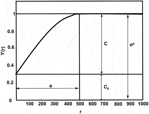
For a regular distribution of data, the choice of the interpolation method is crucial. In this study, we used the Kriging method. This method is based on the statistical theory of random functions and on the spatial correlation of data defined by a variogram $\mathit{\gamma }\left(\mathit{r}\right)$ (Oyoa et al. 2012). This function defines the relationship between the variance and the distance of the values observed in the different locations. In practice, the experimental variogram is calculated using the formula given by equation (30)(30) $\mathit{\gamma }\left(\mathit{r}\right)=\frac{1}{2\mathit{N}\left(\mathit{r}\right)}\sum _{\mathit{i}=1}^{\mathit{N}\left(\mathit{r}\right)}{\left[Z\left(x_i+\mathit{r}\right)-\mathit{Z}\left(x_i\right)\right]}^2$(30) .

(30) $\mathit{\gamma }\left(\mathit{r}\right)=\frac{1}{2\mathit{N}\left(\mathit{r}\right)}\sum _{\mathit{i}=1}^{\mathit{N}\left(\mathit{r}\right)}{\left[Z\left(x_i+\mathit{r}\right)-\mathit{Z}\left(x_i\right)\right]}^2$(30)

where, $\mathit{r}$ is the distance between the couples of measurement points, $\mathit{N}\left(\mathit{r}\right)$ is the number of pairs of points with distance$\mathit{r}$. For this experimental variogram model, an admissible theoretical model is fitted by quantifying several parameters. Among these parameters, we have the scope $\left(\mathit{a}\right)$ which corresponds to the distance where the correlation between the observation points becomes null, the step $\left({\sigma }^2\right)$which corresponds to the sum of the nugget effect $\left(C_0\right)$and the variance $\left(\mathit{C}\right)$ a random variable (Figure 2).

Figure 2. Graph of the experimental variogram and its characteristics.

The main theoretical admissible variogram models are given by the equations below.

• -Spherical

(31) $\mathit{\gamma }\left(\mathit{r}\right)=\mathit{C}\left[\frac{3\mathit{r}}{2\mathit{a}}-\frac{1}{2}{\left(\frac{r}{a}\right)}^3\right]+C_0\mathit{if}0<\mathit{r}<\mathit{a}$(31)

(32) $\mathit{\gamma }\left(\mathit{r}\right)=\mathit{C}+C_0\mathit{ifr}\ge \mathit{a}$(32)

- Exponential

(33) $\mathit{\gamma }\left(\mathit{r}\right)=\mathit{C}\left[1-\mathit{exp}\left(-\frac{3\mathit{r}}{a}\right)\right]+C_0$(33)

- Gaussian

(34) $\mathit{\gamma }\left(\mathit{r}\right)=\mathit{C}\left[1-\mathit{exp}(-3\left(\frac{r}{a}{)}^2\right)\right]+C_0$(34)

- Penta-spherical

(35) $\mathit{\gamma }\left(\mathit{r}\right)=\mathit{C}\left[\frac{15\mathit{r}}{8\mathit{a}}-\frac{5}{4}{\left(\frac{r}{a}\right)}^3+\frac{3}{8}{\left(\frac{r}{a}\right)}^5\right]+C_0\mathit{ifr}<\mathit{a}$(35)

(36) $\mathit{\gamma }\left(\mathit{r}\right)=\mathit{C}+C_0\mathit{ifr}\ge \mathit{a}$(36)

The choice of the appropriate theoretical model is made by a graphic study or by a comparative study between the values of the standard deviation of the experimental and theoretical variogram. The expression of the standard deviation ($\mathrm{RMS}$) is given by the following equation:

(37) $\mathit{RMS}=\sqrt{\sum _{\mathit{i}=1}^n{\left({\mathit{\gamma }}_{\mathit{experimental}}-{\gamma }_{\mathit{theoretical}}\right)}^2}$(37)

With, ${\gamma }_{\mathit{experimental}}$ and ${\gamma }_{\mathit{theoretical}}$ respectively the experimental and theoretical values of variograms.

2.4. 3D representation method of the basement-sediment contact

The 3D representation method of the basement-sediment contact presented in this work consists first of separating the Bouguer anomaly into regional and residual anomalies using a Matlab code taking into account the different equation (equation 1(1) $\mathit{r}\left(x_i,y_i\right)=\sum _{\mathit{r}=0}^n\sum _{\mathit{s}=0}^n{c}_{\mathit{rs}}{x}^r{y}^s$(1) , 2(2) $\mathit{E}=\sum _{\mathit{i}=1}^N{\left[r\left(x_i,y_i\right)-\mathit{b}\left(x_i,y_i\right)\right]}^2$(2) , 3(3) $\frac{\mathrm{\partial E}}{\mathrm{\partial }{\mathit{C}}_{\mathit{rs}}}=0$(3) , 4(4) $\mathit{r}{ }^{\mathrm{\prime }}\left(x_i,y_i\right)=\mathit{b}\left(x_i,y_i\right)-\mathit{r}\left(x_i,y_i\right)$(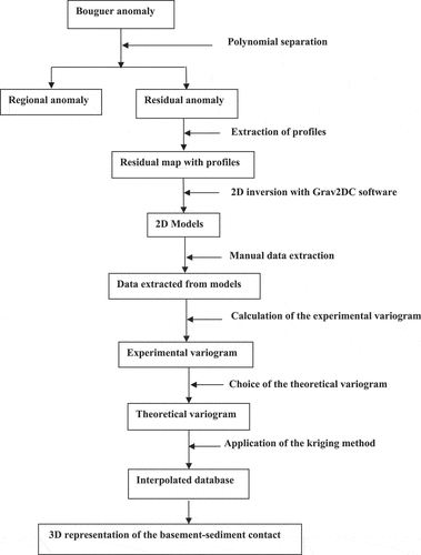4) ) of the separation (Nlen Wounle et al. 2023). Then, make 2D inversion using the Grav2DC software of Cooper (2003) on the profiles executed on the residual anomaly map at the level of the sedimentary zone considered. For a better view, these profiles are plotted perpendicular to the elongation of anomalies and are spaced at a constant pitch. They must have the same direction and the same length. Then, extract the data along these profiles in order to have the 2D models. After having obtained the theoretical structures corresponding to each profile, the data of each structure (position along the x-, y- and z-axes which describe the shape of the sedimentary basin in an orthogonal reference frame whose axes are the direction of the profiles, the direction of the elongation of the anomaly and the direction perpendicular to the surface) are extracted and all put in an EXCEL file. These data being irregularly distributed, an interpolation by the geostatistical kriging method is applied in order to make them regular. This after having determined the theoretical variogram adapted thanks to the experimental variogram. A 3D representation of the basement-sediment contact is then obtained from this database interpolated using the Surfer software. Figure 3 shows the flowchart of the 3D representation method of the base-sediment contact.

Figure 3. Flowchart of the 3D representation method of the base-sediment contact.

To verify the reliability and efficiency of this method, we first apply it to synthetic data produced by a prism in order to have a view of the contact between the prism and the basement. Then, we apply it to data from the transition zone between the Benue and Lake Chad basins to represent the basement-sediment contact in this zone.

3. Synthetic application

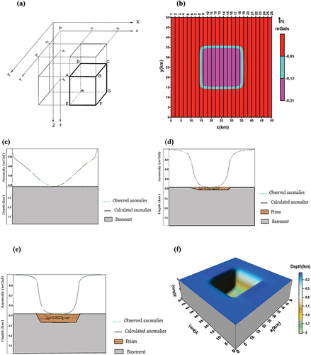
A model of the vertical prism (Figure 4a) is designated here to test the basement-sediment contact. In this part, we present the application of the proposed method to a prism of the sedimentary nature deposited in the basement. The characteristics of this prism are density:$2700\mathrm{kg}/{\mathrm{m}}^3$; length :$20\mathrm{km}$; width : $20\mathrm{km}$ height : $2\mathrm{km}$. Practical results are presented and briefly discussed to demonstrate the success and effectiveness of this method. The theoretical gravity anomalies produced by the prism were calculated using a MATLAB code based on the formula of Banerjee and Das Gupta (1977). These gravity data are generated on a surface of $50\times 50\mathrm{k}{\mathrm{m}}^2$ with a step of 1 km. Figure 4b shows the theoretical gravity anomaly map obtained from the synthetic data produced by the prism. This map presents the effect of the prism expressed here at low amplitudes concentrated in the centre of the map due to the choice of a positive value of density. The different colours observed in this map correspond to the anomaly values. The values between −0.21 and −0.13mGal corresponding to the purple part represent the effect of the prism, those between −0.13 and −0.05mGal corresponding to the green part, represent the edge effect of the prism and those located beyond −0.05 corresponding to the red part, represent the presence of the base. In this anomaly map, we have plotted 26 profiles of S-N direction, the same size ($50\mathrm{km}$) and equidistant from each other by $2\mathrm{km}$ (Figure 4b).

Figure 4. (a) Representation of the prism, (b) 2D anomaly map with profiles, (c) 2D model of profile 1, (d) 2D model of profile 8, (e) 2D model of profile 14, (f) 3D representation of the base-prism contact.

To have 2D models of the profiles crossing the zone representing the effect of the prism as well as those located outside this zone, we extracted the data along these profiles. The Grav2DC software of Cooper (2003) allows us to obtain these models.

Figure 4c represents the shape of the 2D models of the profiles distant from the anomaly representing the effect of the prism (profiles 1, 2, 3, 4, 5, 6, 7, 20, 21, 22, 23, 24, 25 and 26). In this model, we only observe the basement; the effect of the prism is not perceptible due to the distance of the profiles represented by this model.

Figure 4d represents the shape of the 2D model of the profiles near the anomaly (profiles 8 and 19). We notice a slight appearance of the prism effect.

Figure 4e makes visible the effect of the prism. The 2D model represented by this figure is that of the profiles which cross the anomaly produced by the prism (profiles 9, 10, 11, 12, 13, 14, 15, 16, 17 and 18). The closer we get to the anomaly, the greater the effect of the prism. The straight and cubic shapes of the prism are not noticeable in these different models. All the anomaly curves of these models have a parabolic shape because the 2D modelling is done along the profile and therefore does not show the exact shape of the prism.

To obtain the 3D representation of the contact between the prism and the basement, we superimposed the data extracted from the 2D models. These data represent a set of coordinates (x, y, z) which describe the shape of the anomalies, the direction of the profiles and the direction perpendicular to the surface. The interpolation of these data by the Kriging method with the exponential variogram model allows obtaining the 3D representation.

Figure 4f shows the 3D representation of the contact between the prism and the basement. The hollow in the centre represents the prism in the basement, the grey part represents the basement and the blue part represents the ground surface. The analysis of this model allows us to better observe the cubic shape and position of the prism in the basement and to find its characteristics that were unnoticed in 2D models, namely shape (cubic), length (20 km), width (20 km), height (2 km), depth (0 km), which demonstrates the efficiency and the power of the method to represent with more precision the contact between basement and prism.

4. Field application: the basement-sediment contact of transition zone between the Benue and Lake Chad basins (North Cameroon)

In this section, we apply the method presented previously to the transition zone between the Benue and Lake Chad basins (North Cameroon) to represent in 3D the basement-sediment contact of this zone.

4.1. Geological setting

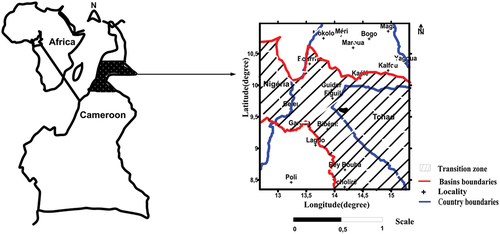
The transition zone between the Benue basin and the Lake Chad basin is located in North Cameroon. It covers an area of about $2000\mathrm{k}{\mathrm{m}}^2$ (Figure 5). Centred at ${14}^{\circ }{00}^{\prime }$East longitude and $9^{\circ }{66}^{\prime }$ North latitude, it straddles between the north and far north regions of Cameroon. It is bound to the South by the Benue basin, to the North by the Lake Chad basin, to the East by Chad and to the West by Nigeria.

Figure 5. Location of the transition zone between the Benue and Lake Chad basins.

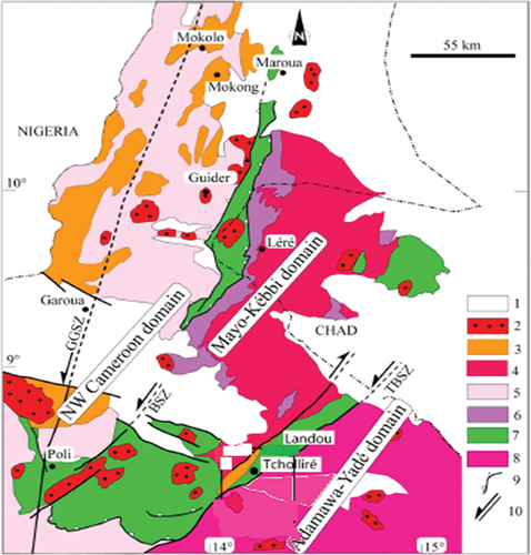
The geology of this zone is dominated by a Precambrian basement and a broad sedimentary cover. Most geological substratums are crystalline and metamorphic basement. Thus, the basement is essentially constituted of crystalline rocks (various granites and metamorphic rocks) attributed to the Lower Precambrian (Figure 6). It finds in this zone, shales, granitoids, slates, micaceous quartzites, muscovites chists, biotite and amphibole. We also note the presence of gneisses, migmatites, diorites, anatexies, syenites, basalts and schists (Penaye et al. 2006). The intrusive granites crop out extensively in the study area. These rock units form the basement complex below the sediments and are thus termed the gneissic-granitic basement. Old and young sediments cover this area. The dominant sedimentary facies are conglomerates and coarse grained alluvial sandstones. These sandstones are often rich in iron oxides, and they crop out throughout the entire study area (Bessong et al. 2015). Previous geological and geophysical work shows that this zone is also characterised by numerous major and minor lineaments with the NW-SE and NNE-SSW main directions. Watercourses such as Benue, Logone, Mayo-kebi, Mayo-Louti and Mayo-Tsanaga characterise the hydrology of this zone.

Figure 6. Geological sketch map of the study area (modified from Penaye et al. 2006).

(1) Post-Pan-African sediments, (2) Late to post-tectonic Pan-African granitoids, (3) Syntectonic granite, (4) Mayo-Kebbi batholith: tonalite, trondhjemite and granodiorite, (5) medium- to high-grade gneisses of the Northern domain, (6) Mafic to an intermediate complex of the Mayo-Kebbi domain (metadiorite and gabbro-diorite) and amphibolites, (7) Neoproterozoic low-to medium-grade volcano-sedimentary sequences of the Poli-Léré Group, (8) Remobilised Palaeoproterozoic Adamawa-Yadé domain, (9) Thrust front, (10) Strike-slip fault: TBSZ = Tcholliré- Banyo shear zone; GGSZ = Godé-Gormaya shear zone.

4.2. Gravity data

The gravity data used in this work have been acquired from the Earth Gravitational Model 2008 (EGM2008). Satellite missions have been launched in the years 2000 to measure the global gravitational field. The potential field obtained has been used to derive a variety of global geopotential models, which express the Earth’s gravitational field in terms of harmonic basis functions. EGM2008 which derived from EGM96, has been corrected for long wavelengths greater than 300 km. This model is complete to degree and order $2159$ and contains additional coefficients up to degree $2190$ and order $2159$ (Pavlis et al. 2012). This model provides gravity data with a spatial resolution of 5 min of arc. It integrates land, airborne and maritime gravity data as well as data derived from satellite altimetry. In this study, a $4096$ point dataset is used.

4.3. Results and discussions

4.3.1. Bouguer anomaly map

This map (Figure 7) shows positive and negative anomalies with values between $-85$ and $+5\mathrm{mGal}$. The positive anomalies are present to the north of the locality of Poli, north-east of Tcholiré, north-east of Bibémi and in the locality of Yagoua. The negative anomalies cover the Lagdo axis, Rey Bouba, west of Tcholire and west of Bibemi. They are more representative in the localities of Bourrha, Guider, Mokolo, Meri, Kalfou and parts of Nigeria. The comparison of this map to the geology shows that the positive anomalies could be linked to the presence of intrusive bodies (basalts, migmatites, gneiss, etc.). The negative anomalies are associated with granitic rocks and sedimentary formations composed mainly of sandstone, marl and sand present in these areas.

Figure 7. Bouguer anomaly.

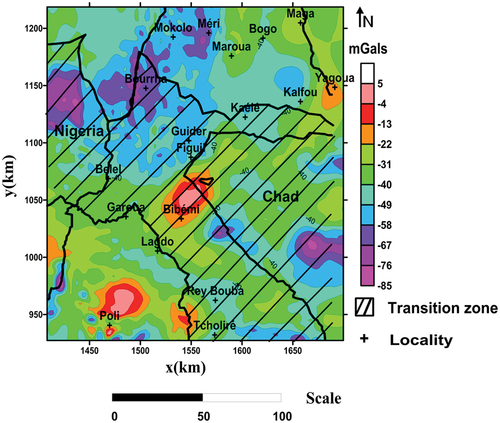
In order to have a better view of the basement-sediment contact in this area, the residual anomalies have been separated from the regional anomalies.

4.3.2. Separated maps

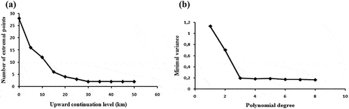
For good separation, it is judicious to have the best degree of separation. For this, upward continuations of the Bouguer anomaly map are calculated at increasing altitudes ranging from $0$ to $50\mathrm{km}$ in steps of $5\mathrm{km}$. For each upward-continued map, the number of extrema (points where the gradient is zero) $\mathrm{N}$ is counted. The height above that, the number $\mathrm{N}$ remains approximately constant, is $\mathrm{H}=\mathit{\hspace{0.17em}}30\mathrm{km}$ (Figure 8a). After applying polynomial smoothing on surfaces of degree $\mathit{d}$ and calculating the minimum variance for each degree, we obtain the graph of the minimum variance as a function of the degree of the polynomial (Figure 8b). This graph gives us the optimum degree of separation which is estimated at $\mathrm{n}=3$.

Figure 8. (a) Graph of variation of the number of extrema according to the upward continuation height, (b) graph of the variance according to the degree of the polynomial.

The regional anomaly map (Figure 9a) shows heavy and light anomalies elongated in the E-W direction. These anomalies express, respectively, the effects of intrusive rocks and granitic rocks deep in the crust. The heavy anomalies are located in the Benue basin and light ones in the Lake Chad basin. In this map, the transition zone between the two basins coincides with the zone which separates the heavy anomalies from the light anomalies, which allows us to suspect the existence of discontinuities at depth in this zone.

Figure 9. (a) Graph of variation of the number of extrema according to the upward continuation height, (b) graph of the variance according to the degree of the polynomial.

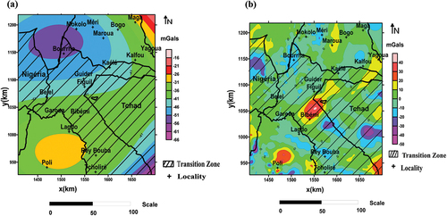
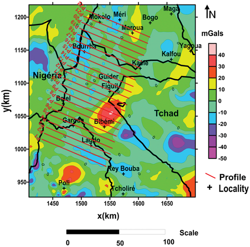
The residual anomaly map (Figure 9b) highlights positive and negative anomalies, with values varying between $-50$ and $40\mathrm{mGal}$ from general directions E-W and NW-SE. These anomalies reflect the effects of superficial and shallow geological structure. They are separated by important gradients indicating the presence of lineaments in the subsurface. The presence of sedimentary deposits in the Precambrian rocks of the basement could be the cause of the negative anomalies covering the localities of Bourrha, Guider, Figuil, Mokolo and Meri.

To better characterise and have a better view of these sedimentary deposits responsible for negative anomalies, 2D models and 3D representation were carried out.

4.3.3. 2D gravity modelling

In this work, we are interested in the residual anomaly map, the one that gives the best geological information. This is why, we have drawn on this map $22$ profiles of $120\mathrm{km}$ long from SE-NW directions crossing an area of sedimentary deposits. They are equidistant from each other by $10\mathrm{km}$ (Figure 10). Then, we extracted the data along these profiles. To get an idea of the shape of sedimentary deposits along each profile, 2-D modelling was done using the Grav2Dc software of Cooper (2003). By adjustment, we obtain the final model when the calculated anomaly is closest to the observed anomaly. The gravimetric effects of the simple structures used in this software were formulated by Hubert (1948) and Talwani et al. (1959) for graphical and analytical approaches, respectively.

Figure 10. Residual anomaly map of study area showing the profiles.

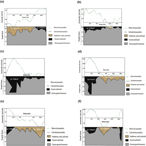
Figure 11 shows the 2D model examples of profiles 1; 5; 7; 10; 15 and 21. In addition to the shape, 2D modelling gives us the extension, depth and density contrast of the sedimentary deposits of each profile. Taking into account the fact that we are in a transition zone between two sedimentary basins whose geology is dominated by a Precambrian basement and a sedimentary cover, we considered a land model whose host is granite-gneissic; the sediments are sandstone in nature. Geology allows us to fix the contrasts of the density of bodies. Thus, the density contrast between the set made up of sand, marl, sandstone and the granite-gneissic basement is $-0.1\mathrm{g}/\mathrm{c}{\mathrm{m}}^3$. The transition zone between the two basins has a granite-gneissic basement with a density of $2.55\mathrm{g}/\mathrm{c}{\mathrm{m}}^3$. The models obtained show sediment deposits of maximum depth $6.3\mathrm{km}$, maximum extension $85.6\mathrm{km}$ and contrast density $-0.1\mathrm{g}/\mathrm{c}{\mathrm{m}}^3$. This contrast allows us to say that the deposits are composed of sandstone, sand and marl with an average density of $2.45\mathrm{g}/\mathrm{c}{\mathrm{m}}^3$. Note also that the heavy masses have a density contrast of $0.1\mathrm{g}/\mathrm{c}{\mathrm{m}}^3$. They are composed of basalt, and syenite with an average density of $2.65\mathrm{g}/\mathrm{c}{\mathrm{m}}^3$. These heavy masses could be an obstacle to communication between the two sedimentary basins.

Figure 11. 2D model examples of profiles (a) 1; (b) 5; (c) 7; (d) 10; (e) 15 and (f) 21.

4.3.4. Choice of the appropriate variogram

In this work, to obtain the theoretical variogram model adapted to the data extracted from the 2D models, a comparative study between the different theoretical variograms and the experimental variogram was made. 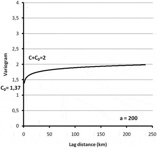The experimental variogram is calculated from equation (30)(30) $\mathit{\gamma }\left(\mathit{r}\right)=\frac{1}{2\mathit{N}\left(\mathit{r}\right)}\sum _{\mathit{i}=1}^{\mathit{N}\left(\mathit{r}\right)}{\left[Z\left(x_i+\mathit{r}\right)-\mathit{Z}\left(x_i\right)\right]}^2$(30) using a Matlab code. The obtained results allowed for plotting the experimental variogram (Figure 12), and the curve was then smoothed. From this variogram, we obtain the following parameters: $\mathit{a}=200$; ${\sigma }^2=\mathit{C}+C_0=2$; $C_0$ = 1.37.

Figure 12. Experimental variogram.

The theoretical variograms of the models (spherical, exponential, Gaussian and penta-spherical) were calculated using the parameters obtained from the experimental variogram. The results from these calculations are classified according to the distance, then grouped into intervals centred on increasing multiples of distance $\mathrm{r}=5\mathrm{km}$. Table 1 shows the different experimental and theoretical variogram values obtained. We noticed that these values increase with the distance. Statistical analysis of this table shows that the different values of the theoretical variograms are close. The difference between the means of these values is small. The value of the standard deviation of each variogram model is calculated using equation (37)(37) $\mathit{RMS}=\sqrt{\sum _{\mathit{i}=1}^n{\left({\mathit{\gamma }}_{\mathit{experimental}}-{\gamma }_{\mathit{theoretical}}\right)}^2}$(37) . These values are shown in the last line of the table. A comparison of these values shows that the standard deviation of the exponential variogram model is the lowest. Thus, this model is considered as the one which gives the best variogram. We also demonstrate this by a comparative study between the different theoretical variogram curves. Figure 13 shows the superposition of the different theoretical and experimental variogram curves as a function of distance. An analysis of these curves shows that it is the curve of the theoretical exponential variogram model that comes closest to the experimental curve.

Figure 13. The different types of variogram.

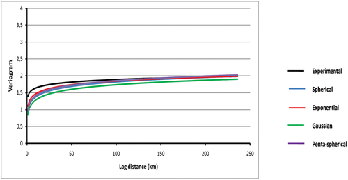
Table 1. Comparative study of the different types of variogram.

Distance	Experimental	Spherical	Exponential	Gaussian	Penta-spherical
2.5	1.13	1.38	1.39	1.37	1.38
7.5	1.63	1.40	1.43	1.37	1.41
12.5	1.59	1.42	1.47	1.37	1.44
17.5	1.62	1.45	1.51	1.38	1.46
22.5	1.84	1.47	1.54	1.39	1.49
27.5	1.92	1.49	1.57	1.40	1.52
32.5	1.97	1.51	1.61	1.41	1.55
37.5	1.92	1.54	1.63	1.42	1.58
42.5	2.03	1.56	1.66	1.44	1.61
47.5	2.07	1.58	1.68	1.46	1.63
52.5	2.14	1.61	1.71	1.48	1.66
57.5	2.08	1.63	1.73	1.49	1.68
Standard deviation		1.33	1.07	1.66	1.22

4.3.5. 3D representation of the basement-sediment contact

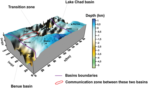
A 3D representation of the basement-sediment contact was carried out using $559$ data collected on 2D models of the profiles that constitute our sedimentary network. These data are represented along $\mathit{x}$, $\mathit{y}$ and $\mathit{z}$ coordinates (where $\mathit{x}$ and $\mathit{y}$ represent the surface coordinates and $\mathit{z}$ the depth of the sediment deposits). After interpolation of these data by the geostatistical method of ordinary kriging with the exponential variogram model, we obtain the 3D representation of the basement-sediment contact of our study area (Figure 14). This representation shows sediment deposits with a maximum depth of approximately $5.5\mathrm{km}$ around the locality of Lagdo. This depth is high for sedimentary deposits located at the ends of the study area, that is to say in the two sedimentary basins. At the level of the Benue basin, this depth is around $4\mathrm{km}$, this is in agreement with the results of the work of Kamgia et al. 2005. Below the sediments, we observe the basement, which is thicker in the centre than at the ends of the study area. We note that sedimentary deposits are shallower and almost absent in the north of Garoua, in Bibemi, Kaele and Maroua; this is explained by the rise of the basement and the presence in these regions of metamorphic and igneous rocksin particular, gneiss, basalt and syenite as shown in the geology map. This scarcity of sedimentary deposits, the low value of depth of deposits in these regions and the high thickness of the basement prevent contact between the two basins and therefore constitute great barriers to communication between the two basins. However, this model shows that other studies in the area between Garoua, Belel and Figuil could open up avenues for communication between these two basins.

Figure 14. 3D representation of the basement-sediment contact.

5. Validation of results

In this study, a new 3D representation method of gravity anomalies in order to show the basement-sediment contact in a sedimentary zone is developed and presented. To verify its validity and efficiency, this method was first applied to synthetic data produced by a prism to represent in 3D the contact between the prism and the basement. The model obtained allowed us to better observe the position of the prism in the basement and to find its different characteristics, namely: shape, length, width, height and depth. After these satisfactory results, the method was applied to the gravity data of the transition zone between the Benue basin and the Lake Chad basin to have a better view of the basement-sediment contact of this zone. The geological map presented above shows that this area is dominated by a Precambrian basement consisting essentially of crystalline rocks (various granites and metamorphic rocks) (Figure 6) and a cover layer composed of post-Pan-African sediments (Penaye et al. 2006). The results of the 2D models of the structures of the area obtained in this work are in agreement with this geology. They show that the basement is made up of granite and gneiss and the sediment deposits are made up of sandstone, marl and sand. The sedimentary region of the Benue trough located in south of Garoua observed in the geological map is clearly visible in the 2D and 3D models obtained. The maximum depth of these sediments estimated at more than 4 km around the locality of Lagdo in this work correlates with the results of the work of Kamgia et al. (2005) and Mouzong et al. (2014) which demonstrated that the area has a granito-gneissic basement and the surface is covered with sediments mainly consisting of sandstones whose depth is beyond 4 km. The models confirm that the two large basins in the study area are indeed sedimentary zones as observed in geological and gravity maps. The area at the north of Garoua, in Bibémi, Kaélé and Maroua are almost devoid of sediments as shown on the geological map, which is explained by the rise of the basement and the presence in these regions of metamorphic and igneous rocksin particular, gneiss, basalt and syenite, which represents a barrier to communication between the two basins. Compared to other 3D inversion methods, approaches and tools integrated in software, the method presented in this work is fast, simple, efficient and allows to have a better view of the basement-sediment contact in a sedimentary zone and to better characterise it. The 2D inversion method of Talwani et al. (1959) and Bott (1960) shows the geometric structure of the sedimentary deposit only along a profile, but the 3D representation method presented in this work shows the complete geometric structure of the sedimentary ditch.

From the representation method of the basement-sediment contact developed in this work, it is possible to:

• - Estimate the geometric parameters of a sedimentary ditch using the gravity field;

• - Estimate the maximum sediment depth in sedimentary basins that may be petroleum reservoirs;

• - In hydrogeology, this work would make it easy to choose, for example, the prospecting drilling points which must be located in places where the depth of the sediments is great;

• - In civil engineering, this work makes it possible to master the implementation of structures in sedimentary areas.

• - It also allows knowing if it is possible to have contact or communication between two sedimentary basins.

6. Conclusion

In this study, a fast method of 3D representation of the basement-sediment contact in a sedimentary zone is developed. This method is based on the polygonal model of Talwani et al. (1959) and stacked rectangular prism model of Bott’s (1960). It consists of separating the Bouguer anomaly into regional and residual anomaly by the polynomial method to better locate the sediment deposits. Then, 2D inversion on several profiles plotted on the residual anomaly map is realised. The interpolation of the data collected from these models by the geostatistical method of Kriging allows obtaining the 3D model of the basement-sediment contact of the area. To verify its validity and efficiency, this method was first applied to synthetic data produced by a prism to represent in 3D the contact between the prism and the soil. After obtaining satisfactory results, the method was applied to the gravity data of the transition zone between the Benue basin and the Lake Chad basin in order to have a better view of the basement-sediment contact of this zone. The results obtained show that the study area is constituted of sediment deposits which are mainly composed of sandstones. The maximum depth of these sediments is approximately 5.5 km around the locality of Lagdo. These deposits are less thick and almost absent in the north of Garoua, in Bibemi, Kaele and Maroua. The results of this study are not only in agreement with the information published and available in the study area but provide more information on the structure of the basement of this region and may be useful in prospecting work mining, civil engineering and hydrology.

Disclosure statement

No potential conflict of interest was reported by the author(s).

References

- Banerjee B, Das Gupta SP. 1977. Gravitational attraction of a rectangular parallelepiped. Geophysics. 42(5):1053–1055. doi: 10.1190/1.1440766.
- Bessong M, Mbesse CO, Ntsama AJ, Hell JV, Abderrazack ELA, Fontaine C, Nolla JD, Dissombo EAN, Eyong JT, Mvondo OF. 2015. Mineralogy and clay minerals distribution in the Benue through, Northern Cameroon (W. Africa): diagenetic significance. Int J Applied Research. 1(11):1–8.
- Bott MHP. 1960. The use of rapid digital computing methods for direct gravity interpretation of sedimentary basins. Geophys J R Astron Soc. 3(1):63–67. doi: 10.1111/j.1365-246X.1960.tb00065.x.
- Cai H, Zhdanov M. 2015a. Application of Cauchy-type integrals in developing effective methods for depth-to-basement inversion of gravity and gravity gradiometry data. Geophysics. 80(2):G81–G94. doi: 10.1190/geo2014-0332.1.
- Cai H, Zhdanov M. 2015b. Modeling and inversion of magnetic anomalies caused by sediment–basement interface using three-dimensional Cauchy-type integrals. IEEE Geosci Remote S. 12(3):477–481. doi: 10.1109/LGRS.2014.2347275.
- Chen S, Zhang J, Shi YL. 2008. Gravity inversion using the frequency characteristics of the density distribution. Appl Geophys. 5(2):99–106. doi: 10.1007/s11770-008-0018-2.
- Cooper GRJ. 2003. GRAV2DC for windows user’s manual (version 2.10). Johannesburg: Geophysics Department, University of the Witwatersrand.
- Fadakinte I. 2022. 3D geophysical mapping of the subsurface to support urban water planning: a case study from Simawa, Nigeria. NRIAG J Astron Geophys. 11(1):120–131. doi: 10.1080/20909977.2022.2031555.
- Giao PH, Chung SG, Kim DY, Tanaka H. 2003. Electric imaging and laboratory resistivity testing for geotechnical investigation of Pusan clay deposits. J Appl Geophys. 52(4):157–175. doi: 10.1016/S0926-9851(03)00002-8.
- Hinze WJ, Von Frese RRB, Saad AH. 2013. Gravity and magnetic exploration principles, practices, and applications 515. (NY): Cambrige University Press. 10.1017/CB09780511843129.
- Hubert MK. 1948. A line integral method of computing the gravimetric effects of two dimensional masses. Geophysics. 13(2):215–225. doi: 10.1190/1.1437395.
- Kamguia J, Manguelle-Dicoum E, Tabod CT, Tadjou JM. 2005. Geological models deduced from gravity data in the Garoua basin, Cameroon. J Geophys Eng. 2(2):147–152.
- Krige DG. 1951. A statistical approach to some basic mine valuation problems on the witwatersrand. J Chem, Metal and Min Soc South Africa. 52:119–139.
- Mouzong MP, Kamguia J, Nguiya S, Shandini Y, Manguelle-Dicoum E. 2014. Geometrical and structural characterization of garoua sedimentary basin, Benue trough, North Cameroon, using gravity data. J Biol and Earth Sciences. 4(1):25–33.
- Nazanin M, Seyed-Hani MA, Vahid EA. 2021. Improved 3D Cauchy-type integral for faster and more accurate forward modeling of gravity data caused by basement relief. Pure Appl Geophys. 178(1). doi: 10.1007/s00024-020-02635-5.
- Njandjock NP, Oyoa V, Ndougsa MT, Bisso D. 2012. C++ code for separation of regional and residual of potential field. Greener J Phys Sci. 2(4):120–130.
- Nlen Wounle BY, Oyoa V, Njandjock NP, Doka YS. 2023. A new MATLAB code for locating lineaments in the earth’s crust from gravity data—a case of the transition zone between Benue basin and Lake Chad basin: cameroon. Arab J Geosci. 16(12). doi: 10.1007/s12517-023-11797-0.
- Oyoa V, Njandjock NP, Bisso D, Diab AD, Manguelle DE. 2012. A geostatistical approach to map gravity data over Logone-Birni sementary basin (Chad-Cameroon). Eur J Sci Res. 93(2):183–189.
- Pavlis NK, Holmes SA, Kenyon SC, Factor JK. 2012. The development and evaluation of the earth gravitational model 2008 (EGM2008). J Geophys Res: Atmosph. 117(B4):1–38. doi: 10.1029/2011JB008916.
- Penaye J, Kröner A, Toteu SF, Van Schmus WR, Doumnang JC. 2006. Evolution of the Mayo Kebbi region as revealed by zircon dating: an early (ca. 740Ma) Pan-African magmatic arc in southwestern chad. J Afr Earth Sci. 44(4–5):530–542. doi: 10.1016/j.jafrearsci.2005.11.018.
- Sultan N, Voisset M, Marsset B, Marsset T, Cauquil E, Colliat JL. 2007. Potential role of compressional structures in generating submarine slope failures in the Niger Delta. Mar Geol. 237(3–4):169–190. doi: 10.1016/j.margeo.2006.11.002.
- Talwani M, Worzel J, Ladisman M. 1959. Rapid gravity computations for two dimensional bodies with application to the Mendocino submarine fracture zone. J Geophys Res. 64(1):49–59. doi: 10.1029/JZ064i001p00049.
- Witter JB, Siller DL, Faulds JE, Hinz NH. 2016. 3D geophysical inversion modeling of gravity data to test the 3D geologic model of the Bradys geothermal area, Nevada, USA. Geotherm Energy. 4(1). doi: 10.1186/s40517-016-0056-6.
- Zeng H. 1989. Estimation of the degree of polynomial fitted to gravity anomalies and its application. Geophys Prospect. 37(8):959–973. doi: 10.1111/j.1365-2478.1989.tb02242.x.
- Zhao G, Chen B, Chen L, Liu J, Ren Z. 2018. High accuracy 3D Fourier forward modeling of gravity field based on the Gauss-FFT method. J Appl Geophys. 150:294–303. doi: 10.1016/j.jappgeo.2018.01.002.
- Zhdanov MS. 2015. Inverse theory and application in geophysics. Amsterdam: Elsevier.