An automatic new approach to gravity anomaly’s profile separation, inversion and interpretation, using an infinite horizontal slab model

ABSTRACT

The goal of this research is to develop a new, fast-applying, non-conventional 2D semi-inversion technique that uses data from a previously known control point (e.g. a borehole). The method successfully separated a digitised profile over the Bouguer gravity anomaly map into its components, each of which corresponded to a rock formation being prior chosen from a borehole or control point. The importance of this technique stems from its capacity to automatically analyse the shape of the Bouguer gravity anomaly, as well as its propriety, approximation and given accepted equivalent geological cross-section, utilising an infinite slab model. A preliminary synthetic guidance model (SGM) in this proposed new method is being created from borehole data to simulate the homogeneous density distribution of the rock formations that fill a hypothetical sedimentary basin so that it represents to far extent the history of the region’s sedimentation process. The theoretical gravitational effect for each rock formation is estimated using the infinite horizontal slab model for all rock formations of such a hypothetical basin model. The total of these gravitational effects is utilised to invert any gravity profile that crosses the Bouguer gravity anomaly map. The gravity anomalies of the Bouguer profile are then separated and inverted into the comparable rock formation thicknesses or/and depths tracked along the gravity’s profile using a simple method. The technique was tested on a synthetic model, a synthetic noisy contaminated model, and real data from two different field cases with different geological and lithological characteristics. The first was in the Tucson Basin in Southeast Arizona, USA, and the second on the Mors Salt Dome in North Jutland, Denmark. The method has demonstrated results comparable with prior known information of the borehole existing in the study areas.

KEYWORDS:

• Depth
• semi-inversion
• infinite horizontal slab
• Bouguer
• model

1. Introduction

Gravity method is one of the geophysical passive methods that is relatively low-cost, non-destructive to the environment and is used often in the pre-exploration stages as a reconnaissance tool to research the distribution shape of density or density-contrast variations in the stratigraphy of the rocks in the subsurface of the Earth. The purpose of the gravity technique is to obtain an accurate image, as close to reality as possible, of the Earth’s subsurface geological structures, such as folds, fractures, etc., as well as recognisable and clear stratigraphic features, such as salt domes, sand lenses, etc.

Overall, the gravity survey, processing, correction, separation, inversion and interpretation are integrated steps, where each step builds upon the previous one and requires specialised knowledge and experience to ensure the accuracy and reliability of the results. Each step plays an essential role in obtaining accurate and significant results. The survey step involves measuring and recording the gravity data at specific locations covering the entire target area. This data is then processed to remove the errors due to any external factors and noise influences on the observed gravity measurements. The correction step adjusts the data for known density variations in the Earth’s crust. This correction helps to remove the effect of the Earth’s topography and allows geophysicists to obtain more accurate measurements of the local gravity field, which can provide important information about the structure and composition of the Earth’s subsurface. Separation is then used to separate the total corrected gravity effects into its gravity effect components, each one equivalent to a certain anomalous source element (e.g. a certain rock formation). Inversion is a mathematical technique that transforms the separated gravity anomaly data into an equivalent model of the densities distribution shape of the subsurface stratigraphic rocks. Interpretation of either qualitative or quantitative is used to provide valuable insights into subsurface geology and help guide exploration and development efforts.

After latitude, elevation (free air), Bouguer and terrain corrections, the observed gravity data are used to calculate the sum of all effects, from the top of rock formations to the rock basement. The present technique is interested in the interpretation of the stratigraphic features and rock formations that are confined between the Earth’s surface and basement rocks or the deepest rocks of the Earth’s crust, as reference levels to measure the gravity effects and any concerning physical parameters. For instance, the density contrast of rock formations in this research indicates the difference in density between the density of the rock formation and the density of the basement rocks. The Bouguer gravity anomaly is an important gravity measurement used in geophysics to estimate the density, thickness and shape of subsurface rock formations.

In this technique, the separation and inversion process is carried out automatically upon a profile’s cross-section of a Bouguer gravity anomaly map. Based on the assumption that the density distribution of the subsurface can be approximated by a set of horizontal rock formations, each with its own constant density and density contrast with basement rock, and each of these formations contributes to the total gravity anomaly measured on the Earth’s surface. Under this assumption, the Earth’s subsurface is divided into a set of rock formations, which are assumed to have constant densities and are equivalents to discrete infinite horizontal slabs. The vertical densities and thicknesses of these rock formations are determined based on prior information, such as geological and geophysical data. After the separation of the total gravity anomaly measured on the Earth’s surface into an equivalent gravity effect of each an infinite horizontal slab, the equivalent density and thickness of each rock formation are estimated by solving an inverse problem for the measured gravity anomaly data.

The understanding of gravity and its related concepts has changed and evolved over time as a result of new discoveries, research, observations and theoretical frameworks. For example, the utility of the concept of Zero-Offset Gravity Measurement (ZOGM) introduced by Abdelfattah (2022) has led to improved constrained inversion to reduce the ambiguity in gravity anomaly interpretation, using simple geometrical models. Therefore, in the present method, an infinite horizontal slab was used as one of the direct or forward geometrical shape modelling. This application of the concept removes the effect of dip-angle from calculations and also provides a more efficient and reliable inversion. Also, the accuracy of the estimated density distribution depends on the number and thickness of the equivalent layers, as well as the quality and resolution of the Bouguer gravity anomaly data.

However, the accuracy of the estimated density and thickness of each rock formation depend on the number of equivalent rock formations chosen from the borehole, as well as the quality and resolution of the observed gravity data. Therefore, ambiguity is the most challenging problem when interpreting gravity data, which researchers still face, where the modelling of potential-field data is considered to be a non-linear problem. However, a unique solution may be found, when assigning a simple geometrical shape to the causative body (Salem et al. 2010). Fortunately, almost most of the geological structures can be approximated, by one or more of the available simple geometrical shape models, to represent the causative sources for gravity anomalies (Abdelfattah 2022).

The inverse gravimetric problem, namely the determination of a subsurface mass density distribution corresponding to an observed gravity anomaly, has an intrinsic non-uniqueness of its solution (e.g. Al-Chalabi 1971). Several authors have researched the inversion of gravity data attempting to reduce non-uniqueness (or ambiguity) since the last decade to the present day (e.g. Al-Chalabi 1971; Oldenburg 1974; Fournier and Krupicka 1975; Parker 1975, 1977; Verma et al. 1976; Pedersen 1977; Baldi and Unguendoli 1978; Rao et al. 1990, 1994; Lee and Biehler 1991; Mickus and Peeples 1992; Vasco et al. 1993; Chakravarthi 1995; Boschetti et al. 1997; Abdeslem 2000; Burger et al. 2006; Chappell and Kusznir 2008; Silva et al. 2010; Zhou 2010; Wahyudi et al. 2017; Abdelfattah 2022).

An infinite horizontal slab model has been used by several researchers and authors primarily as a conventional classical method such as Bouguer’s correction or reduction of the gravity measurements for regional and investigation studies in the field of geodesy (e.g. LaFehr 1991; Nowell 1999). The purpose of the Bouguer correction is to remove the gravity of materials that are not of interest, such as the topography of the Earth’s surface (Bullard 1936). Also, an infinite horizontal slab model is used in the application of borehole gravity meters (BHGM) information evaluation to estimate bulk density from which porosity and fluid saturation are determined (Li and Chouteau 1999). An infinite horizontal slab is also used as an interpretive technique such as gravity stripping or gravity interpretation by stripping (e.g. Woollard 1938; Hammer 1963; Hinpkin and A 1983; Miroslav et al. 2013) and determination of the depth of bedrock (e.g. Kick 1985; Abbott and Louie 2000).

2. Materials and methodology

Microsoft Excel, Surfer 15 Golden Software and the free software CurveSnap V 1.0 were used in this paper, and the program’s main algorithm code is written using MATLAB R2014b for the Bouguer gravity anomaly separation and inversion gravity anomaly along the profile to correspond with their borehole known rock formations.

The author of this paper has proposed a 2D new approach to gravity anomaly separation and interpretation, in which a way to invert profile data gravitational anomalies using an infinite slab model was presented. This method was constrained by prior known information (control points or drilled wells) to reduce the ambiguity problem of interpreting gravity anomaly data to far extent. A preliminary Synthetic Guidance Model (SGM) is utilised, which is created from the borehole’s data to simulate the homogeneous density distribution of the rock formations that fill a hypothetical sedimentary basin of the being studied area. Then, an infinite horizontal slab model was used to calculate the gravity effect for the SGM. This gravity effect is used for the separation as well as the inversion process of the cross-section along geological and/or stratigraphic features of the Bouguer gravity anomaly map.

It is important to take into consideration that the Bouguer gravity data do not provide information on the actual density of each isolated rock formation. Instead, they only provide information on the density contrast of the whole sedimentary cover with basement rocks (or the deepest rocks in the Earth’s crust). So, the basement rock in this research was used as a reference for calculating the density contrasts of each isolated rock formation of its overlying deposited rock formations. Hence, the present method is based on the assumption that the gravitational effects of each rock formation represent an isolated causative source, confined between the Earth’s surface and basement rocks. Therefore, the gravity effect of each isolated rock formation is calculated from its corresponding infinite horizontal slab model (Abdelfattah 2022). In this approach, the total gravity effect at any Earth’s surface point is equal to the sum of all vertical superimposed gravitational effects sources, and such slab models represent those rock formations.

2.1. Formulation of the equation of an infinite horizontal slab model

Figure 1 illustrates the gravity effect calculated on Earth’s surface at any point P (x, y) caused by a subsurface infinite horizontal slab of density material (ρ) in g/cm³ unit, thickness ($\mathit{h}$) in km unit and its density contrast (∆ρ) also in g/cm³ unit, which is obtained by using the following equation:

(1) $g_z=2\mathit{\pi G}\Delta \mathit{\rho h}$(1)

Figure 1. Illustration of an infinite horizontal slab model.

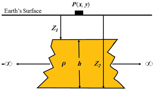
where ($g_z$) represents the calculated vertical gravity response for the infinite horizontal slab in m. Gal (10⁻⁵ m/s²) unit, at the observation surface station P (x, y), ($\mathit{G}$) is the Universal Gravity Constant 6.67 × 10⁻³ N.km/s⁻², where N refers to Newton or force unit, obtained as following:

(2) $\mathit{h}=\left(z_{\mathit{i}+1}-z_i\right)$(2)

where $z_{\mathit{i}+1}$ and $z_i$ are the bottom depth and the top depth of the slab, respectively, and their index number $\mathit{i}=1,2,3\dots \mathit{N}.$

It is worth mentioning that the density contrast in this paper is equal to the difference between the slab’s material (formation rock) density ${\rho }_{\mathit{slab}}$ and the basement rock density ${\rho }_{\mathit{basement}}$, given as:

(3) $\mathrm{\Delta \rho }={\rho }_{\mathit{slab}}-{\rho }_{\mathit{basement}}$(3)

2.2. The zero-offset gravity measurement (ZOGM) concept

It is obvious from equation (1)(1) $g_z=2\mathit{\pi G}\Delta \mathit{\rho h}$(1) that the gravity effect of the vertical component of gravity attraction ($g_z$) at any point of the Earth’s surface ($\mathit{x}=0$), vertically above the infinite horizontal slab, depends upon its material’s density contrast with basement rocks and its thickness. This meets or satisfies the conditions of ZOGM’s concept (given by Abdelfattah 2022). The ZOGM’s point represents the maximum value of the gravitational effect, at the surface of the Earth from the centre of any simple geometrical-shaped body, which can therefore be used as a forward gravity model to calculate the gravitational effect of any subsurface point that acts as a causative source gravity anomaly. Each of the Bouguer values can therefore be viewed as a single isolated maximum value (or ZOGM’s point). 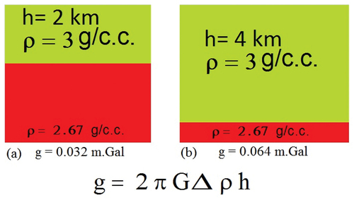Furthermore, the density contrast ($\mathrm{\Delta \rho }$) and the thickness of the slab ($\mathit{h}$) have a direct correlation with the gravitational effect. The concept of ZOGM serves as the foundation for distinguishing between two slabs with similar density contrasts with basement rocks, but different thicknesses, as illustrated in Figure 2, where the two slabs of the same density contrast with bedrocks 0.33 g/cm³ have different thicknesses of 2 km and of 4 km and give gravity effects of 0.032 and 0.064 m. Gal, respectively.

Figure 2. The vertical gravity effects of the different slabs at different thicknesses and the same density contrasts.

2.3. Synthetic guide model (SGM) of Rock’ density distribution fill the basin

Based on the deposition history principle, described by Steno’s Superposition Law describes, a Synthetic Guide Model (SGM) for any area could be built using prior known borehole data or the available subsurface information for a study location (Table 1). This SGM simulates the homogeneous density distributions of the rock formations that fill the basin (Figure 3). Hence, the results of calculating gravitational effects on the Earth’s surface of the SGM can be obtained using borehole information and by applying the infinite horizontal slab model (Table 2), using equation 1(1) $g_z=2\mathit{\pi G}\Delta \mathit{\rho h}$(1) . Later on, those gravity calculations could be used to estimate the rock formations’ thicknesses and depths of the Bouguer anomaly gravity map’s profile by the gravity inversion process.

Figure 3. Homogeneous density distributions or SGM model.

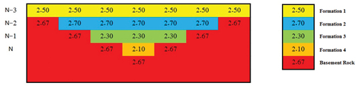
Table 1. Hypothetical drilled well data (SGM) of a three-layer model.

Formations	z (km)	h (km)	D (g/cm^3)
S.L.	0.00	0.00	0.00
A	8.00	8.00	3.00
B	10.00	2.00	3.10
C	12.00	2.00	3.20
Basement	20.00	10.00	2.67
∑∑		20.00

Table 2. Calculated total gravity effects of the SGM.

Formation	gB_SGM (m. Gal)
S.L.	0.00
A	0.11
B	0.03
C	0.04
Basement

SGM = Synthetic Guide Model.

2.4. Theory and the inversion process mathematically

The purpose of the present research is mainly an attempt to solve the ambiguity in gravity interpretation. Additionally, it aims to resolve inaccuracies associated with the interpretation of salt dome structures, in particular, due to their physical properties.

The total gravity effects of the SGM that do build from prior known data of the area and that consisting of rock formations deposited above basement rocks can be calculated by a little modification of equation (1)(1) $g_z=2\mathit{\pi G}\Delta \mathit{\rho h}$(1) . Hence, an appropriate and general formula, for forward gravity calculating, is obtained as follows:

(4) $g_{\mathit{Bt}}\left(\mathit{i}\right)=\sum _{\mathit{i}=1}^{N}2\mathit{\pi GAV}\_\mathit{DC}\left(\mathit{i}\right)\mathit{h}\left(\mathit{i}\right)$(4)

where $g_{\mathit{Bt}}\left(\mathit{i}\right)$ is the total gravity anomalies of each of the observation points $x_c\left(\mathit{i}\right)$, on the surface, along the vertical axis of the thicknesses $\mathit{h}\left(\mathit{i}\right)$ of the subsurface slabs, as the $\mathit{AV}\_\mathit{DC}\left(\mathit{i}\right)$ represents the average vertical densities-contrasts of the slab’s density with basement rock density, such that the indices i = 1, 2, 3…N and N are the numbers of vertically superimposed horizontal slabs representing rock formations. In other words, the total of gravity at any point on the Earth’s surface is considered to be a summation of all vertical points inside a series of superimposed infinite horizontal slabs, each of which represents rock formation.

It is worth mentioning that the used density contrasts in this paper are the Average Vertical Density Contrasts (AVDC = $\mathit{AV}\_\mathit{DC}$), which are obtained from the average density contrasts $\overline{\mathrm{\Delta \rho }}\left(\mathit{i}\right)$ as in the next equation (5), at every observation point on the surface as follows:

(5) $\overline{\mathrm{\Delta \rho }}\left(\mathit{i}\right)=\sum _{\mathit{i}=1}^N\frac{\mathrm{\Delta \rho }\left(\mathit{i}\right)}{N}$(5)

where $\mathrm{\Delta \rho }\left(\mathit{i}\right)$ is the density contrast of formations with basement rock.

Then, the AVDC (i) is obtained as follows:

(6) $\mathit{AV}\_\mathit{DC}\left(\mathit{i}\right)=\overline{\mathrm{\Delta \rho }}\left(\mathit{i}\right)-{\rho }_{\mathit{basement}}$(6)

Equation (4)(4) $g_{\mathit{Bt}}\left(\mathit{i}\right)=\sum _{\mathit{i}=1}^{N}2\mathit{\pi GAV}\_\mathit{DC}\left(\mathit{i}\right)\mathit{h}\left(\mathit{i}\right)$(4) is rearranged to calculate the thicknesses by inverting the gravitational anomaly, as follows:

(7) $\mathit{h}\left(\mathit{i}\right)=\mathit{abs}\left(g_{\mathit{Bt}}\left(\mathit{i}\right)/\left(2\mathit{\pi GAV}\_\mathit{DC}\left(\mathit{i}\right)\right)\right)$(7)

Hence, the $g_{\mathit{Bt}}\left(\mathit{i}\right)$ can be inverted into their corresponding rock formation thicknesses $\mathit{h}\mathit{\hspace{0.17em}}\left(\mathit{i}\right)$ by solving equation (7)(7) $\mathit{h}\left(\mathit{i}\right)=\mathit{abs}\left(g_{\mathit{Bt}}\left(\mathit{i}\right)/\left(2\mathit{\pi GAV}\_\mathit{DC}\left(\mathit{i}\right)\right)\right)$(7) , an automatic iterative using an appropriately designed MATLAB algorithm. The rock’s formation depths (including basement rock) can also be estimated along the profile by the following equation:

(8) $\mathit{z}\left(\mathit{i}\right)={\displaystyle \sum {\displaystyle \sum _{\mathit{i}=1}^N\mathit{h}}\left(\mathit{i}\right)}$(8)

The two summation signs in equation (8) mean the cumulative sum of the thicknesses $\mathit{h}\mathit{\hspace{0.17em}}\left(\mathit{i}\right)$ along $\mathit{N}$ row or rock formations numbers ($\mathit{i}$ = 1, 2, 3…, $\mathit{N}$), expressed in MATLAB as $\mathit{\hspace{0.17em}}\mathit{z}\left(\mathit{i}\right)$ = cumsum ($\mathit{h}\mathit{\hspace{0.17em}}\left(\mathit{i}\right)$, 2), and the inverted depth of the basement rock only can be obtained as follows:

(9) $\mathit{z}\_\mathit{basement}=\left(\mathit{abs}\left(\sum _{\mathit{i}=1}^N\mathit{z}\left(\mathit{i}\right))/\mathit{N}\right)\ast 2\right)$(9)

2.4.1. Creating a synthetic geological cross-section (three-layer case)

A synthetic geological cross-section of three rock formations overlying basement rocks at different depths and densities was created (Figure 4). The assumed parameters of those rock formations are in Table 3.

Figure 4. A synthetic geological cross-section of a three-layer case.

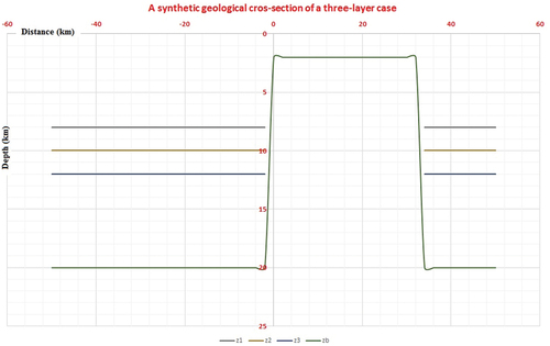
Table 3. The parameters of the three-layer case.

Formation	h_SGM (km)	z_SGM (km)	D (g/cm^3)	Av. D (g/cm^3)	Av. D.C. (g/cm^3)
A	8.00	8.00	3.00	3.00	0.33
B	2.00	10.00	3.10	3.05	0.38
C	2.00	12.00	3.20	3.10	0.43
Basement		20.00	2.67		0.38

SGM = Synthetic Guide Model.

2.4.2. Forward synthetic gravity profile using slab model

The theoretical calculated gravity anomaly profile of synthetic model (Figure 5) represents the gravity response at 51 points on the Earth’s surface ($\mathit{x}\left(\mathit{i}\right)$, $g_{\mathit{Bt}}\left(\mathit{i}\right))$ of the afore-created synthetic geological cross-section, using a horizontal slab model. This was carried out by calculating the gravity at each point for each isolated slab representing a rock formation and then summing the result at each point (represents as a measuring point) to give the total gravity corresponding to the synthetic geological cross-section (Table 4). The total gravity anomaly of SGM $g_{\mathit{Bt}\_\mathit{M}}\left(\mathit{i}\right)$ for density distributions is calculated by modifying the equation (4)(4) $g_{\mathit{Bt}}\left(\mathit{i}\right)=\sum _{\mathit{i}=1}^{N}2\mathit{\pi GAV}\_\mathit{DC}\left(\mathit{i}\right)\mathit{h}\left(\mathit{i}\right)$(4) as follows:

(10) $g_{\mathit{Bt}\_\mathit{M}}\left(\mathit{i}\right)=\sum _{\mathit{i}=1}^{N}2\mathit{\pi GAV}\_\mathit{DC}\left(\mathit{i}\right)h_M\left(\mathit{i}\right)$(10)

Figure 5. The theoretical calculated gravity anomaly profile of a synthetic geological cross-section model.

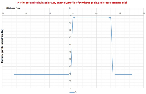
Table 4. The data of the synthetic geological cross-section model.

Xc (km)	h1 (km)	h2 (km)	h3 (km)	hb (km)	z1 (km)	z2 (km)	z3 (km)	zb (km)
−50	8	2	2	8	8	10	12	20
−48	8	2	2	8	8	10	12	20
… …	…	… …	… …	… …	… …	… …	… …	… …
−44	8	2	2	8	8	10	12	20
−42	8	2	2	8	8	10	12	20
−40	8	2	2	8	8	10	12	20
… …	…	… …	… …	… …	… …	… …	… …	… …
−12	8	2	2	8	8	10	12	20
−10	8	2	2	8	8	10	12	20
… …	…	… …	… …	… …	… …	… …	… …	… …
−6	8	2	2	8	8	10	12	20
−4	8	2	2	8	8	10	12	20
−2	8	2	2	8	8	10	12	20
0				2				2
2				2				2
… …	…	… …	… …	… …	… …	… …	… …	… …
10				2				2
22				2				2
… …	…	… …	… …	… …	… …	… …	… …	… …
26				2				2
48	8	2	2	8	8	10	12	20
50	8	2	2	8	8	10	12	20

where $g_{\mathit{Bt}\_\mathit{M}}\left(\mathit{i}\right)$ is the gravity effects, $h_M\left(\mathit{i}\right)$ is the slab SGM’ thicknesses and $\mathit{AV}\_\mathit{DC}\left(\mathit{i}\right)$ is the average vertical density contrasts.

2.4.3. Inversion of the synthetic profile, using slab model

The 2D semi-inversion method is implemented by applying an infinite horizontal slab model for both GSM and synthetic gravity profile, as follows:

2.4.3.1. Depth inversion for SGM

The depth inversion of the gravity response of SGM ($g_{\mathit{Bt}\_\mathit{M}}\left(\mathit{i}\right)$) is obtained as follows:

(11) $h_M\left(\mathit{i}\right)=\mathit{abs}(g_{B{t}_M}\left(\mathit{i}\right))/\left(2\mathit{\pi G}\left(\mathit{AV}\_\mathit{DC}\left(\mathit{i}\right)\right)\right))$(11)

Therefore, the depths are obtained by the following equation:

(12) $z_M\left(\mathit{i}\right)=\sum {\sum }_{i=1}^N{h}_M\left(\mathit{i}\right)$(12)

where $z_M\left(\mathit{i}\right)$ is the inverted depths of $g_{\mathit{Bt}\_\mathit{M}}\left(\mathit{i}\right)$, the two summation signs in the equation (12) mean the cumulative sum of the thicknesses $h_M\mathit{\hspace{0.17em}}\left(\mathit{i}\right)$ along each row or rock formations ($\mathit{i}$ = 1, 2, 3…, $\mathit{N}$) and the inverted basement depth $z_M\_\mathit{basement}$ only is obtained as follows:

(13) $z_M\_\mathit{basement}=\left(\mathit{abs}\left({\sum }_{i=1}^N{z}_M\left(\mathit{i}\right))/\mathit{N}\right)\ast 2\right)$(13)

The results of the inverted SGM are listed in Table 5 and represented in Figure 6.

Figure 6. The inverted depths of SGM.

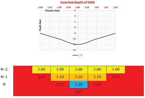
Table 5. The inverted depths of SGM.

Formation	h_SGM (km)	z_SGM (km)
S.L.	0.00	0.00
A	8.00	8.00
B	2.00	10.00
C	2.00	12.00
Basement		20.00

SGM = Synthetic Guide Model.

2.4.3.2. Depth inversion for the synthetic gravity profile

Actually, to invert the synthetic gravity profile data ($g_{\mathit{Bt}}\left(\mathit{i}\right)$), by using the new approach of slab model $g_{\mathit{Bt}\_\mathit{M}}\left(\mathit{i}\right)$, the equations (7), (8) and (9) are modified as follows:

(14) $h_{\mathit{MP}}\left(\mathit{i}\right)=\mathit{abs}(((g_{\mathit{Bt}}\left(\mathit{i}\right)g_{B{t}_M}\left(\mathit{i}\right))/\left(2\mathit{\pi G}\left(\mathit{B}.\mathit{D}\right)\right)\ast \left(\left(\mathit{N}+1\right)/2\right)$(14)

where $g_{\mathit{Bt}}\left(\mathit{i}\right)$ is the synthetic profile gravity anomaly due to the three-layer case structure ($\mathit{N}=3$), $h_{\mathit{MP}}\left(\mathit{i}\right)$ is the slabs thicknesses, $\mathit{B}.\mathit{D}$ is called Balance Density of the total formations and $g_{\mathit{Bt}\_\mathit{M}}\left(\mathit{i}\right)$ is the calculated gravity effect of the SGM.

(15) $\mathit{B}.\mathit{D}=\left(\mathit{AV}\_\mathit{DC}\left(\mathit{i}\right)\right)/{\sum }_{i=1}^N\left(\mathit{AV}\_\mathit{DC}\left(\mathit{i}\right)/\mathrm{N}\right)$(15)

(16) $z_{\mathit{MP}}\left(\mathit{i}\right)=\sum {\sum }_{i=1}^N{h}_{\mathit{MP}}\left(\mathit{i}\right)$(16)

where $z_{\mathit{MP}}\left(\mathit{i}\right)$ is the depths of rock formations (inclusive the basement rock) by using slab model, and the inverted basement depth only is obtained as follows:

(17) ${{\mathit{z}}_{\mathit{MP}}}_{\mathit{basement}}\left(\mathit{j}\right)=\mathit{abs}({\sum }_{j=1}^M{z}_{\mathit{MP}}\left(\mathit{i}\right))$(17)

The result of inversion is summarised in Table 6 and represented as shown in Figure 7.

Figure 7. The inverted depth of synthetic gravity profile.

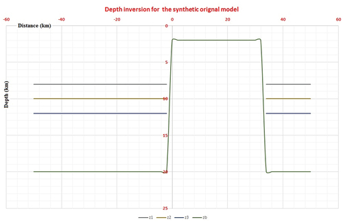
Table 6. The inverted depth of synthetic gravity profile.

Xc (km)	gBt (m.Gal)	h1 (km)	h2 (km)	h3 (km)	hb (km)	z1 (km)	z2 (km)	z3 (km)	zb (km)
−50	0.808269	8	2	2	8	8	10	12	20
−48	0.808269	8	2	2	8	8	10	12	20
… …	… … … .	…	… …	… …	… …	… …	… …	… …	… …
−44	0.808269	8	2	2	8	8	10	12	20
−42	0.808269	8	2	2	8	8	10	12	20
−40	0.808269	8	2	2	8	8	10	12	20
… …	… … … .	…	… …	… …	… …	… …	… …	… …	… …
−12	0.808269	8	2	2	8	8	10	12	20
−10	0.808269	8	2	2	8	8	10	12	20
… …	… … … .	…	… …	… …	… …	… …	… …	… …	… …
−6	0.808269	8	2	2	8	8	10	12	20
−4	0.808269	8	2	2	8	8	10	12	20
−2	0.808269	8	2	2	8	8	10	12	20
0	0.031994				2				2
2	0.031994				2				2
… …	… … … .	…	… …	… …	… …	… …	… …	… …	… …
10	0.031994				2				2
22	0.031994				2				2
… …	… … … .	…	… …	… …	… …	… …	… …	… …	… …
26	0.031994				2				2
48	0.808269	8	2	2	8	8	10	12	20
50	0.808269	8	2	2	8	8	10	12	20

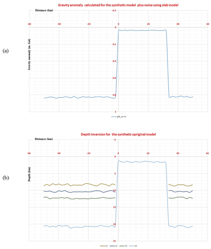
2.4.4. Testing inversion of noisy synthetic gravity profile

For testing the effects of the noise on the efficiency of the present technique, 10% random noise has been added to the synthetic gravity anomaly data (Figure 8), as follows:

(18) $g_{\mathit{Bt}\_\mathit{err}}\left(\mathit{i}\right)=g_{\mathit{Bt}}\left(\mathit{i}\right)+\left(\mathit{RAND}\left(\mathit{i}\right)\ast 0.1\right)$(18)

Figure 8. Gravity effects of the synthetic three-layer case (free-noisy and noisy) and the corresponding inverted depths.

where $g_{\mathit{Bt}\_\mathit{err}}\left(\mathit{i}\right)$ is the output 10% contaminated gravity anomaly of the input gravity anomaly data $g_{\mathit{Bt}}\left(\mathit{i}\right)$, corresponding to each observation point $\left(\mathit{i}=1,2,3,\dots \mathit{N}\right)$.

The corresponding $g_{\mathit{Bt}\_\mathit{err}}\left(\mathit{i}\right)$ values are then used in thicknesses and depths inversion by applying the modified equations (14), (16) and (17), and the following equations are obtained:

(19) $\mathit{h}\_\mathit{noise}\left(\mathit{i}\right)=2\ast \mathit{abs}(g_{\mathit{B}{\mathit{t}}_{\mathit{err}}}\left(\mathit{i}\right)g_{B{t}_M}\left(\mathit{i}\right)))/\left(2\mathit{\pi G}\left(\mathit{B}.\mathit{D}\right)\right)$(19)

where $g_{\mathit{B}{\mathit{t}}_{\mathit{err}}}\left(\mathit{i}\right)$ is the synthetic profile of noise-contaminated gravity anomaly due to a three-layer case structure, $\mathit{h}\mathrm{\_}\mathrm{noise}\left(\mathit{i}\right)$ is the slabs noisy thicknesses and $g_{\mathit{Bt}\_\mathit{M}}\left(\mathit{i}\right)$ is the calculated gravity effect of the SGM.

(20) $z_{\mathit{M}\_\mathit{noise}}\left(\mathit{i}\right)=\sum \sum _{\mathit{j}=1}^M\mathit{h}\_\mathit{noie}\left(\mathit{i}\right)$(20)

where $z_{\mathit{M}\_\mathit{noise}}\left(\mathit{i}\right)$ is the noisy depths of formation rocks (three-layers), and the inverted noise basement depth only is obtained as follows:

(21) ${{\mathit{z}}_{\mathit{M}{\mathrm{\_}}_{\mathit{noise}}}}_{\mathit{basement}}\left(\mathit{i}\right)=\mathit{abs}(\sum _{\mathit{i}=1}^M{z}_{\mathit{M}\_\mathit{noise}}\left(\mathit{i}\right))$(21)

The rock formation noisy depths, and also noise basement depths, in comparison with both free-noisy data and noisy data, respectively (Table 7). In addition, the depths of the original synthetic gravity anomaly data (Figure 8a), and compared with the inversion and tracing of the depth of data being contaminated with 10% random error or noise (Figure 8b). The comparison reveals that the new method is efficient and stable because it depends only on the vertical density contrasts between each isolated rock formation and the basement rocks to separate gravitational anomalies into their corresponding formations.

Table 7. Comparison between the inverted depths of the original gravity data and the noisy gravity data.

Original gravity data						Original gravity data + Random noise
xc (km)	gBt (m. Gal)	z1 (km)	z2 (km)	z3 (km)	zb (km)	gBt_error (m. Gal)	zn1 (km)	zn2 (km)	zn3 (km)	znb (km)
−50	0.808269	8.00	10.00	12.00	20.00	0.839235	8.55	10.32	12.42	20.86
−48	0.808269	8.00	10.00	12.00	20.00	0.833667	8.44	10.17	12.05	20.43
−46	0.808269	8.00	10.00	12.00	20.00	0.826767	8.24	10.30	12.29	20.56
−44	0.808269	8.00	10.00	12.00	20.00	0.828262	8.67	10.44	12.02	20.76
−42	0.808269	8.00	10.00	12.00	20.00	0.840777	8.54	10.24	12.48	20.84
… …	… … … .	… …	… …	… …	… …	… … … .	… … … .	… … … .	… … … .	… … … .
−22	0.808269	8.00	10.00	12.00	20.00	0.828743	8.55	10.01	12.34	20.60
−20	0.808269	8.00	10.00	12.00	20.00	0.825612	8.55	10.55	12.19	20.87
… …	… … … .	… …	… …	… …	… …	… … … .	… … … .	… … … .	… … … .	… … … .
−4	0.808269	8.00	10.00	12.00	20.00	0.838194	8.03	10.48	12.02	20.35
−2	0.808269	8.00	10.00	12.00	20.00	0.829509	8.45	10.05	12.04	20.35
0	0.031994				2.00	0.038367				1.47
2	0.031994				2.00	0.040382				1.69
… …	… … … .	… …	… …	… …	… …	… … … .	… … … .	… … … .	… … … .	… … … .
32	0.031994				2.00	0.038728				1.37
34	0.808269	8.00	10.00	12.00	20.00	0.826079	8.05	10.39	12.43	20.58
… …	… … … .	… …	… …	… …	… …	… … … .	… … … .	… … … .	… … … .	… … … .
48	0.832086	8.00	10.00	12.00	20.00	0.832086	8.69	10.24	12.17	2073
50	0.808269	8.00	10.00	12.00	20.00	0.824678	8.13	10.13	12.02	20.19

3. The steps for implementing 2D semi-inversion

The process of semi-inversion begins with the computation of the theoretical gravity response of the SGM, defined by prior known rock formation’s density distribution from wells of the study area. The general procedures applied to the correcting field gravity (Bouguer gravity) data for the three field cases are summarised in the following steps:

1. Digitised and re-contouring the available Bouguer gravity anomaly map with a proper equal contour interval (m. Gal). Also, the available digitised profile data from any source can be used.

2. Building the SGM for rock formation densities homogeneous distribution of available borehole data.

3. Digitizing gravity anomaly profiles in any of being investigated directions of geological feature as structure fault, lithologic fault or even fault scrape in the area.

4. Interpretation by inverting the profile’s gravity anomaly values at each point automatically into their equivalent rocks’ formation depths values at the same points. By implementation of the proposed MATLAB algorithm that was previously prepared, and

5. Comparing the results with other researchers’ and authors’ methods (only if the results are available).

6. An additional algorithm is particularly added and used in the case of the salt dome’s interpretation (concerning with the shape characterisation).

4. 2D semi-inversion method application in real field cases

The semi-inversion in the present research is considered to be a process of reconstruction of the Earth’s mass density distribution (the tops shapes of formation rocks) from observed Bouguer gravity anomaly through the SGM constructed by a prior known borehole data and using an infinite horizontal slab. By evaluating a synthetic model and a synthetic noise-contaminated model, the effectiveness of the present 2D semi-inversion method was ascertained as shown before in advance. The approach was also used with real data in two field situations with different geological and lithological characteristics. The first application took place in the Tucson Basin in Southeast Arizona, the USA, and the second on the Mors Salt Dome in North Jutland, Denmark.

4.1. The geological cross-section of Tucson Basin, Southeast of Arizona, USA

The Tucson Basin, near Tucson, the largest city in southeast Arizona, lies in the Southern Basin and Range Province and is surrounded by the Sierrita, Tumaccacori, Santa Rita and Rincon Mountains (Figure 9). In previous studies, the Tucson Basin has been referred to as a large graben. Its northeastern margin is known as the Black Mountain fault zone. The graben is filled with pre-Tertiary sediments (Heindl 1959) and volcanic material (Lacy and Morrison 1966).

Figure 9. Reference map showing topography overlain with generalised geology.

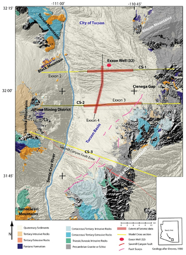
The Tucson Basin is a typical basin and range structural feature, characterized as an alluvium-filled valley surrounded by mountain blocks (Davis 1971). These consist mostly of plutonic igneous and metamorphic rocks, with the exception of the Tucson mountains on the northwestern edge of the basin. These mountains are for the most part volcanic in origin.

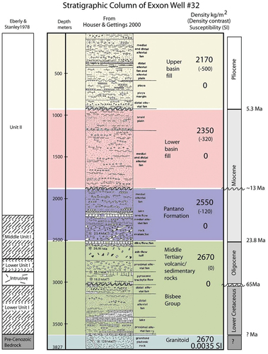
In 1972, Exxon Company, USA, drilled an exploration well (Exxon 32–1) near the centre of the Tucson Basin that penetrated 3,658 m of sedimentary and volcanic rocks above a granitoid basement. The Exxon well was drilled to a total depth of 3,827 m and penetrated the stratigraphic section (Figure 10).

Figure 10. Stratigraphic column of Exxon Well#32_Tucson.

4.1.1. Semi-inversion of the Tucson Basin Bouguer’s gravity profile

The semi-inversion approach steps as previously described were carried out upon one digitised profile AB, across the available Bouguer gravity anomaly map (Figure 11), of the Tucson Basin Area. In addition, the Exxon 32–1 drilled borehole, available for selected rock formation thicknesses (Table 8), was used to build the SGM of distributed densities of the rock formations heterogeneously. The gravity effect values were theoretically calculated for each point of the selected five formations of the SGM of the Tucson Basin Area (Table 9) and its curve of calculated gravity effect (Figure 12).

Figure 11. Bouguer gravity anomaly map of Tucson Basin Area.

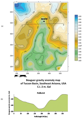
Figure 12. The SGM of the Tucson Basin with its curve of calculated gravity effect.

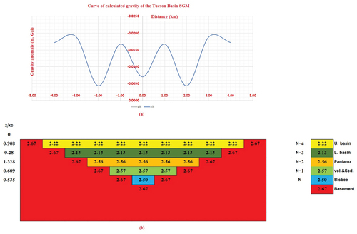
Table 8. The calculated depths inversion of the SGM’s gravity profile (Tucson Basin Area).

Xc (km)	h_SGM (km)	z_SGM (km)
−4	0.908	0.908
−3	0.908	1.916
−2	0.280	2.096
−1	1.328	3.424
0	0.609	4.033
1	1.328	3.424
2	0.280	2.096
3	0.908	1.816
4	0.908	0.908

SGM = Synthetic Guide Model.

Table 9. The EXXON Well-32 available parameters.

Formation	z (km)	h (km)	Density (g/cm^3)	D.C. (g/cm^3)
S.L.	0.000	0.000	0.000	0.000
U. basin	0.000	0.908	2.220	−0.450
L. basin	0.908	0.280	2.130	−0.540
Pantano	1.188	1.328	2.560	−0.110
vol.&Sed.	2.516	0.609	2.570	−0.100
Bisbee	3.125	0.535	2.500	−0.170
Basement	3.660		2.670

D.C.: density contrast = formation density – basement density (g/cm³).

4.1.2. The interpretation of the Tucson basin area and comparing the results

Table 10 presents the results of depths obtained from applying 2D semi-inversion to the Bouguer anomaly profile AB traversing the Tucson Basin Area. The sea level serves as the reference measurement, and the inverted depths of the top rock formations and the basement rocks are as follows: 0.50–0.60 km, 0.70–0.80 km, 1.50–2.70 km, 1.90–2.10 km, 2.20–2.50 km and 2.72–3.08 km, respectively. The corresponding range of negative values for the Bouguer anomaly for sedimentary rocks and basement rocks is 126.59–137.25 m. Gal. The depths of the top formation rocks in Table 10 are represented in Figure 13a before undergoing shape processing. Table 11 represents the top formation rocks when the transition depth values of top formation rocks from high to low (or vice versa) are replaced with an empty value identifying the location of the fault, as shown in Figure 13b. Table 11 represents the depth inversion of gravity profile AB after processing shape 1. Figure 13c, on the other hand, represents Table 11 after processing shape 2, or drawing fault lines. Figure 14 shows the comparison between the seismic section and the inverted depths of the gravity profile AB in the same direction in the Tucson Basin. Thus, the present technique gives a good interpretation and is comparable to far extent with the seismic method.

Figure 13. The depth inversion of the gravity profile AB of the Tucson Basin (processing shape and interpretation).

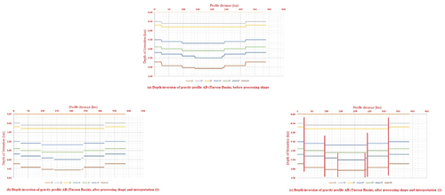
Figure 14. A comparison between the seismic section and the inverted depths of the gravity profile AB in the same direction in Tucson Basin.

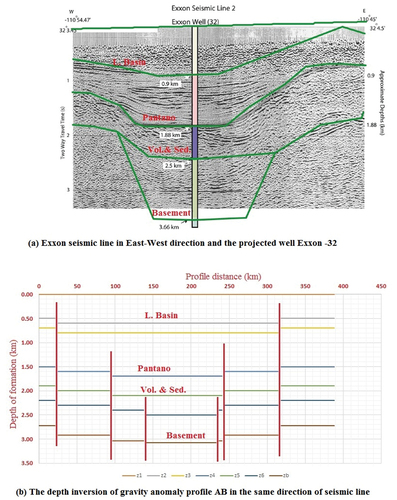
Table 10. The depth inversion of the Tucson Basin’s gravity profile before shape processing.

Xc (km)	gBt (m. Gal)	z1 (km)	z2 (km)	z3 (km)	z4 (km)	z5 (km)	z6 (km)	zb (km)
0	−126.585491	0.00	0.50	0.70	1.50	1.90	2.20	2.72
1.941439876	−126.587203	0.00	0.50	0.70	1.50	1.90	2.20	2.72
23.29727851	−128.2721572	0.00	0.50	0.70	1.50	1.90	2.20	2.72
25.23871838	−128.5927809	0.00	0.60	0.80	1.60	2.00	2.30	2.92
93.18911403	−135.5015774	0.00	0.60	0.80	1.60	2.00	2.30	2.92
95.13055391	−135.6768577	0.00	0.60	0.80	1.60	2.00	2.30	2.92
97.07199379	−135.8530271	0.00	0.60	0.80	1.70	2.10	2.40	3.04
99.01343366	−136.0300858	0.00	0.60	0.80	1.70	2.10	2.40	3.04
137.8422312	−138.2960033	0.00	0.60	0.80	1.70	2.10	2.40	3.04
139.7836711	−138.5424256	0.00	0.60	0.80	1.70	2.10	2.40	3.04
143.6665508	−139.0405531	0.00	0.60	0.80	1.70	2.10	2.50	3.08
145.6079907	−139.4212768	0.00	0.60	0.80	1.70	2.10	2.50	3.08
265.977263	−131.7442765	0.00	0.60	0.80	1.60	2.00	2.30	2.92
267.9187028	−131.711984	0.00	0.60	0.80	1.60	2.00	2.30	2.92
269.8601427	−131.6800614	0.00	0.60	0.80	1.60	2.00	2.30	2.92
273.7430225	−131.7045401	0.00	0.60	0.80	1.60	2.00	2.30	2.92
275.6844624	−131.7341763	0.00	0.60	0.80	1.60	2.00	2.30	2.92
232.9727851	−139.5372107	0.00	0.60	0.80	1.70	2.10	2.50	3.08
234.914225	−138.8928116	0.00	0.60	0.80	1.70	2.10	2.50	3.08
236.8556648	−138.2478934	0.00	0.60	0.80	1.70	2.10	2.40	3.04
242.6799845	−136.3730526	0.00	0.60	0.80	1.70	2.10	2.40	3.04
244.6214243	−135.7602281	0.00	0.60	0.80	1.60	2.00	2.30	2.92
246.5628642	−135.1865433	0.00	0.60	0.80	1.60	2.00	2.30	2.92
316.4546997	−128.8491734	0.00	0.60	0.80	1.60	2.00	2.30	2.92
318.3961396	−128.3940951	0.00	0.50	0.70	1.50	1.90	2.20	2.72
320.3375795	−127.940757	0.00	0.50	0.70	1.50	1.90	2.20	2.72
384.4050954	−123.1067221	0.00	0.50	0.70	1.50	1.90	2.20	2.72
386.3465353	−123.2711698	0.00	0.50	0.70	1.50	1.90	2.20	2.72
388.2879751	−123.4974095	0.00	0.50	0.70	1.50	1.90	2.20	2.72

Table 11. The depths inversion of the gravity profile AB after processing shape 1 and shape 2.

Xc (km)	gBt (m. Gal)	z1 (km)	z2 (km)	z3 (km)	z4 (km)	z5 (km)	z6 (km)	zb (km)
0	−126.585491	0.00	0.50	0.70	1.50	1.90	2.20	2.72
1.941439876	−126.587203	0.00	0.50	0.70	1.50	1.90	2.20	2.72
23.29727851	−128.2721572	0.00
25.23871838	−128.5927809	0.00	0.60	0.80	1.60	2.00	2.30	2.92
93.18911403	−135.5015774	0.00	0.60	0.80	1.60	2.00	2.30	2.92
95.13055391	−135.6768577	0.00	0.60	0.80
97.07199379	−135.8530271	0.00	0.60	0.80	1.70	2.10	2.40	3.04
99.01343366	−136.0300858	0.00	0.60	0.80	1.70	2.10	2.40	3.04
137.8422312	−138.2960033	0.00	0.60	0.80	1.70	2.10	2.40	3.04
139.7836711	−138.5424256	0.00	0.60	0.80	1.70	2.10
143.6665508	−139.0405531	0.00	0.60	0.80	1.70	2.10	2.50	3.08
145.6079907	−139.4212768	0.00	0.60	0.80	1.70	2.10	2.50	3.08
265.977263	−131.7442765	0.00	0.60	0.80	1.60	2.00	2.30	2.92
267.9187028	−131.711984	0.00	0.60	0.80	1.60	2.00	2.30	2.92
269.8601427	-131.6800614	0.00	0.60	0.80	1.60	2.00	2.30	2.92
273.7430225	-131.7045401	0.00	0.60	0.80	1.60	2.00	2.30	2.92
275.6844624	−131.7341763	0.00	0.60	0.80	1.60	2.00	2.30	2.92
326.1618991	−126.5092279	0.00	0.50	0.70	1.50	1.90	2.20	2.72
328.103339	−126.0241903	0.00	0.50	0.70	1.50	1.90	2.20	2.72
330.0447789	−125.5861988	0.00	0.50	0.70	1.50	1.90	2.20	2.72
331.9862187	−125.1509802	0.00	0.50	0.70	1.50	1.90	2.20	2.72
232.9727851	−139.5372107	0.00	0.60	0.80	1.70	2.10	2.50	3.08
234.914225	−138.8928116	0.00	0.60	0.80	1.70	2.10
242.6799845	−136.3730526	0.00	0.60	0.80
244.6214243	−135.7602281	0.00	0.60	0.80	1.60	2.00	2.30	2.92
246.5628642	−135.1865433	0.00	0.60	0.80	1.60	2.00	2.30	2.92
316.4546997	−128.8491734	0.00
318.3961396	−128.3940951	0.00	0.50	0.70	1.50	1.90	2.20	2.72
384.4050954	−123.1067221	0.00	0.50	0.70	1.50	1.90	2.20	2.72
386.3465353	−123.2711698	0.00	0.50	0.70	1.50	1.90	2.20	2.72
388.2879751	−123.4974095	0.00	0.50	0.70	1.50	1.90	2.20	2.72

4.2. The Mors Salt Dome, North Jutland, Denmark

The Mors Salt Dome is one of the well-documented local features in the Danish sedimentary basin, named after the island of Mors situated in the northwestern part of Jutland, Denmark, as shown circled in red (Figure 15a). Mors Island covers an area of about 360 km². It is 10–15 km wide and about 35 km long with the SSW-NNE trend (Jorgensen et al. 2005). The dome-like structure on central Mors is made of chalk, which covers the top of the Erslev salt diaper. On the bedrock map of Mors, the structural contour lines at 25 m intervals show the elevation of the pre-Quaternary surface (Figure 15b).

4.2.1. Depths semi-inversion of the gravity profile of the Mors Salt Dome

Based on the gravity map by Saxov (1956), and revised by (Madirazza 1980; Sharma 1997) and (Abdelfattah 2022), Figure 16a depicts the map of the Bouguer gravity anomaly that covers the Mors Salt Dome region. Also, the digitised gravity profile AB crosses the distinctive shape of the salt dome (Figure 16b). Figure 17a depicts the calculated curve for the gravity effect related to the SGM of the area (Figure 17b). In addition, the Erslv-2 and the Mors-1 are the two available and existing boreholes (Gomm 1982), but the Mors-1 has only been used to construct the SGM, of the area. Table 12 contains the drilling depths of the chosen sedimentary rock formations that are directly deposited above the basement rock and their densities, while the results of the depth inversion of the gravity SGM profile are enclosed in Table 13.

Figure 15. The location of Mors island in the northwestern part of Jutland, Denmark.

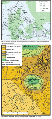
Figure 16. Bouguer gravity anomaly map covering the Mors Salt Dome with a gravity anomaly profile AB.

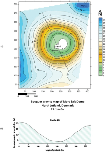
Figure 17. The SGM of the Mors Salt Dome with its curve of calculated gravity effect.

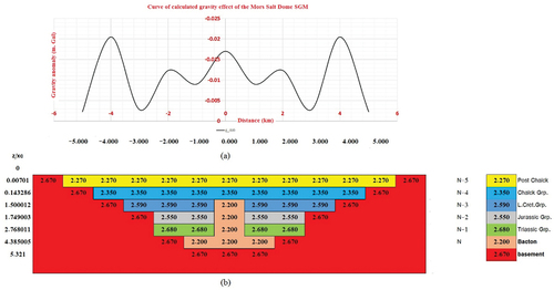
Table 12. The Mors-1 borehole’s data.

Formation	z (km)	h (km)	ρ (gm/cm^3)	Δρ (gm/cm^3)	$\overline{\mathrm{\Delta }\mathit{\rho }}$ (gm/cm^3)
Post Chalk	0.007	0.136	2.270	−0.470	−0.47
Chalk Grp.	0.143	1.357	2.350	−0.390	−0.43
L. Cret. Grp.	1.500	0.249	2.590	−0.150	−0.34
Jurassic Grp.	1.749	1.019	2.550	−0.190	−0.30
Triassic Grp.	2.768	1.617	2.680	−0.060	−0.30
Bacton (Salt)	4.385	0.936	2.200	−0.540	−0.53
Basement	5.500		2.740

Table 13. The calculated depths inversion of the SGM’s gravity profile (Mors Salt Dome).

Xc (km)	h_SGM (km)	z_SGM (km)
−5	0.136	0.136
−4	1.357	1.493
−3	0.249	1.742
−2	1.617	3.359
−1	0.936	4.295
0	0.936	5.231
1	0.936	4.295
2	1.617	3.489
3	0.249	1.742
4	1.357	1.493
5	0.136	0.136

4.2.2. Interpretation of the Mors Salt Dome and comparing the results

One of the characteristics of the salt dome structure is that the top of the salt formation and its overlaying cap rocks have a short, distinct flattened range that is uplifted, and it may represent a major erosional surface, signifying a significant stratigraphic boundary.

In the present technique, it is assumed that the density of salt is roughly constant in depth between the top and the bottom or base of the salt formation, and the underlying basement rock does not contribute to pushing up the salt. Figure 18a,b represent the preliminary display of the resulting depth inversion of the gravity profile AB (Table 14), revealing the pull-up of both the bottom formation of salt and its underlying basement rock, as well as an abnormal reduction in the thickness of the salt body structure, which should be corrected.

Figure 18. The depth inversion of the gravity profile AB of the Mors Salt Dome (processing shape and interpretation).

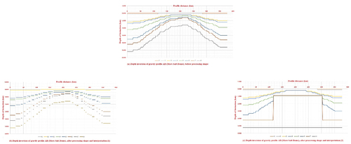
Table 14. The depth inversion of the Mors Salt Dome’s gravity profile before shape processing.

Xc (km)	gBt (m.Gal)	z1 (km)	z2 (km)	z3 (km)	z4 (km)	z5 (km)	z6 (km)	z7 (km)	zb (km)
0	21.23519477	0.000	0.100	1.200	1.400	2.200	3.500	4.200	5.200
1.891480389	21.18056057	0.000	0.100	1.200	1.400	2.200	3.500	4.200	5.200
5.674441168	21.07062606	0.000	0.100	1.200	1.400	2.200	3.500	4.200	5.200
7.565921557	21.01719022	0.000	0.100	1.200	1.400	2.200	3.500	4.200	5.200
18.91480389	20.68714284	0.000	0.100	1.200	1.400	2.200	3.500	4.200	5.200
20.80628428	20.62626215	0.000	0.100	1.200	1.400	2.200	3.500	4.200	5.200
49.17849012	18.75173204	0.000	0.100	1.100	1.300	2.000	3.100	3.800	4.800
51.06997051	18.53108658	0.000	0.100	1.000	1.200	1.900	3.000	3.700	4.633
115.3803037	9.793542177	0.000	0.100	0.600	0.700	1.100	1.700	2.000	3.067
117.2717841	9.587452767	0.000	0.000	0.500	0.600	1.000	1.600	1.900	2.867
119.1632645	9.382378506	0.000	0.000	0.500	0.600	1.000	1.600	1.900	2.867
285.6135388	10.04287097	0.000	0.100	0.600	0.700	1.100	1.700	2.100	3.100
287.5050192	10.29155657	0.000	0.100	0.600	0.700	1.100	1.700	2.100	3.100
376.4045975	18.24794817	0.000	0.100	1.000	1.200	1.900	3.000	3.600	4.600
378.2960779	18.31195154	0.000	0.100	1.000	1.200	1.900	3.000	3.600	4.600

4.2.3. Correction of the Salt Bottom Formation (CSBF)

The CSBF is a step processing for the cases of the salt domes (or the similar structures of diapers) carried out to overcome errors in the inverted depth results and the resulting reduction in the actual thickness of the salt due to the pushing-up of the bottom of the salt formation and the basement rock underlay it. In case the basement rock is not contributing tectonically to pushing the salt up, the depth correction of the bottom of the salt formation is done. By adding and implementing a new algorithm to the main used Matlab program code of depth inversion process, to delineate the edges or the salt dome lateral boundaries. This algorithm depends on a feature unique to the salt dome, which is that the rocks of the cap formations are almost flat, which means that any change in the depths of the rocks adhering to the top of the salt dome can be monitored on the horizontal scale and inferred from it on the two edges of the salt dome. The next stage is replacing the depths between the two edges of the salt dome by adding the depths of all rock formations at the first or second edge and dividing them by the number of rock formations. Therefore, this value represents the top of the salt dome, while the base of the salt dome is the average value of its depths before the two edges.

Automatically, the horizontal range for the vertical sides of the salt dome was delineated its limit as between $x_c$ = 11.380 km, and corresponding anomaly $g_{\mathit{Bt}}$ = 9.794 m.Gal and $x_c$ = 285.614 km, and corresponding anomaly $g_{\mathit{Bt}}$ = 10.429 m.Gal and the depth of the top salt formation are estimated to be 0.886 km, in the mentioned range. Table 15 lists the results of depth inversion of the Mors Salt Dome’s gravity profile after shape processing (1). Figure 18c shows the interpretation of depth inversion of the gravity profile AB after processing the shape of the salt dome by correcting the error in the depth of the bottom salt formation to 4.200 km and the depth of the underlying basement rock to 5.200 km in the limited area of the dome. Table 16 lists the results of depth inversion of the Mors Salt Dome’s gravity profile after shape processing (2)

Table 15. The depth inversion of the Mors Salt Dome’s gravity profile after shape processing (1).

Xc (km)	gBt (m.Gal)	z1 (km)	z2 (km)	z3 (km)	z4 (km)	z5 (km)	z6 (km)	z7 (km)	zb (km)
0	21.23519477	0.000	0.100	1.200	1.400	2.200	3.500	4.200	5.200
1.891480389	21.18056057	0.000	0.100	1.200	1.400	2.200	3.500	4.200	5.200
5.674441168	21.07062606	0.000	0.100	1.200	1.400	2.200	3.500	4.200	5.200
7.565921557	21.01719022	0.000	0.100	1.200	1.400	2.200	3.500	4.200	5.200
18.91480389	20.68714284	0.000	0.100	1.200	1.400	2.200	3.500	4.200	5.200
20.80628428	20.62626215	0.000	0.100
49.17849012	18.75173204	0.000	0.100
51.06997051	18.53108658	0.000	0.100	1.000	1.200	1.900	3.000
115.3803037	9.793542177	0.000	0.100	0.600	0.700	1.100	1.700	2.000	3.067
117.2717841	9.587452767	0.000
119.1632645	9.382378506	0.000	0.000	0.500	0.600	1.000	1.600	1.900	2.867
285.6135388	10.04287097	0.000	0.100	0.600	0.700	1.100	1.700	2.100	3.100
287.5050192	10.29155657	0.000	0.100	0.600	0.700	1.100	1.700	2.100	3.100
376.4045975	18.24794817	0.000	0.100	1.000	1.200	1.900	3.000	3.600	4.600
378.2960779	18.31195154	0.000	0.100	1.000	1.200	1.900	3.000	3.600	4.600

Table 16. The depth inversion of the Mors Salt Dome’s gravity profile after shape processing (2).

Xc (km)	gBt (m.Gal)	z1 (km)	z2 (km)	z3 (km)	z4 (km)	z5 (km)	z6 (km)	z7 (km)	zb (km)
0	21.23519477	0.000	0.100	1.200	1.400	2.200	3.500	4.200	5.200
1.891480389	21.18056057	0.000	0.100	1.200	1.400	2.200	3.500	4.200	5.200
5.674441168	21.07062606	0.000	0.100	1.200	1.400	2.200	3.500	4.200	5.200
7.565921557	21.01719022	0.000	0.100	1.200	1.400	2.200	3.500	4.200	5.200
18.91480389	20.68714284	0.000	0.100	1.200	1.400	2.200	3.500	4.200	5.200
20.80628428	20.62626215	0.000	0.100	1.200	1.400	2.200	3.500	4.200	5.200
49.17849012	18.75173204	0.000	0.100	1.100	1.300	2.000	3.100	4.200	5.200
51.06997051	18.53108658	0.000	0.100	1.000	1.200	1.900	3.000	4.200	5.200
115.3803037	9.793542177	0.000	0.100	0.600	0.700	1.100	1.700	4.200	5.200
117.2717841	9.587452767	0.000	0.000	0.500	0.600	0.893	0.893	0.893	5.200
119.1632645	9.382378506	0.000	0.000	0.500	0.600	0.893	0.893	0.893	5.200
285.6135388	10.04287097	0.000	0.100	0.600	0.700	0.893	0.893	0.893	5.200
287.5050192	10.29155657	0.000	0.100	0.600	0.700	0.893	0.893	0.893	5.200
376.4045975	18.24794817	0.000	0.100	1.000	1.200	1.900	3.000	4.200	5.200
378.2960779	18.31195154	0.000	0.100	1.000	1.200	1.900	3.000	4.200	5.200

The inverted formation rocks’ depths of Mors Salt Dome of the gravity profile AB are comparable to a far extent with the interpretation of corresponding the seismic section (after Kreitz 1982; LaFehr 1982; Sharma 1986) in the same direction as shown in Figure 19. The comparison results of the other authors (LaFehr 1982; Sharma 1986; Aghajani et al. 2009; Hajian and Shirazi 2015; Abdelfattah 2022a) with the new approach and the outcomes of the other methods are included in Table 17.

Figure 19. A comparison between a seismic section and the inverted depth gravity profile in the same direction at Mors Salt Dome.

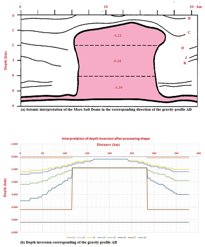
Table 17. Comparative results of the Mors Salt Dome case study, Denmark.

The author(s)	Year	Method	Gravity anomaly type (m.Gal)	Top of salt (km)	Bottom of salt (centre of shape) (km)
LaFehr	1982	Well Logging	BHGM	0.900–1.100	4.385
Sharma	1986	Sphere	Residual	1.000	4.800
Aghajani et al.	2009	NFG	Residual	–	4.700
Hajian and Shirazi	2015	GRNN	Bouguer	–	4.820
Abdelfattah	2022	Sphere	Bouguer		4.030–4.240
Present research	2023	An infinite horizontal slab	Bouguer	0.886	4.200

BHGM: Bore Hole Gravity Meter. NFG: Normalized Full Gradient. GRNN: General Regression Neural Networks.

5. Discussion

The technique proved that it is not impossible to overcome or even reduce the ambiguity in gravity interpretation if the restricting conditions could be taken into consideration and satisfied as hereinafter: First, ensure that the gravity measurements were appropriately measured and corrected. Second, it assumes that the observed gravity anomaly at Earth’s surface equals the sum of all causal point sources rock formations vertically stacked one on top of the other down the vertical axis extent from Earth’s surface to the basement rocks (or deepest rock of the Earth’s crust). Finally, the inversion technique is calculating the gravity effect of the SGM using one of the geometries of a known forward gravity model, such as an infinite horizontal slab, as in the present research, and multiplying by the observed gravity profile’s points using a balanced density contrast.

6. Conclusions

The application of the new approach in real field areas has demonstrated comparable values in calculated rock formations’ thicknesses with those observed in drilled boreholes. Furthermore, apart from the method’s accuracy, and stability, the method simulates in a way similar to the tracing of rock formations from borehole data to the seismic cross-section in the seismic interpretation process. As a result, the method can be recommended as a reconnaissance tool in a preliminary petroleum bid-round evaluation phase and prior to seismic surveys, where it will lower the price of geophysical exploration. Additionally, it aids in detecting the nearest real shape of the salt dome from the Bouguer gravity anomaly. The salt domes are very important for either petroleum exploration or the disposal of radioactive waste.

Acknowledgments

The author sincerely first thanks Prof. Dr. Gad El-Qady, the president of the National Research Institute of Astronomy and Geophysics (NRIAG), Egypt, for his encouragement and support of the researchers. The author also expresses gratitude to NRIAG Journal, Dr. Editor-in-Chief and Editors, Taylor & Francis Online, for helping and directing during writing of this paper. The gratitude extends to the reviewers for their valuable advice and constructive criticism. Prof. Dr. Khaled Essa is acknowledged for his encouragement, and the author also acknowledges his family, especially his wife, for providing a proper environment for carrying out this research.

Disclosure statement

No potential conflict of interest was reported by the author.

References

- Abbott RE, Louie JN. 2000. Depth to bedrock using gravimetry in the Reno and Carson City, Nevada, area basins. Geophysics. 65(2):340–350. do i: 1 0.1190/1.1444730.
- Abdelfattah DM. 2022. A new approach automatic separation of the Bouguer gravity anomaly, using a new concept for 2D-Semi-inversion of the sphere-shaped model. NRIAG J Astron Geophys. 11(1):257–281. doi: 10.1080/20909977.2022.2072083.
- Abdelfattah DM. 2022. New semi-inversion method of Bouguer gravity anomalies separation. In: Gravitational field. IntechOpen. doi: 10.5772/intechopen.101593.
- Abdeslem JG. 2000. 2-D inversion of gravity data using sources laterally bounded by continuous surfaces and depth-dependent density. Geophysics. 65(4):1128–1141. ID: 4769. doi: 10.1190/1.1444806.
- Aghajani H, Moradzadeh A, Zeng H. 2009. Estimation of depth to salt domes from normalized full gradient of gravity anomaly and examples from the USA and Denmark. J Earth Sci. 20(6):1012–1016. doi: 10.1007/s12583-009-0088-y.
- Al-Chalabi M. 1971. Some studies relating to nonuniqueness in gravity and magnetic inverse problem. Geophysics. 36(5):835–855. Corpus ID: 119861663. doi: 10.1190/1.1440219.
- Baldi P, Unguendoli M. 1978. Inversion of gravity profiles by polynomial method. Geophys Prospect. 26(1):247. doi: 10.1111/j.1365-2478.1978.tb01590.x.
- Boschetti F, Dentith M, List R. 1997. Inversion of potential field data by Genetic Algorithm. Geophys Prospect. 45(3):461–478. doi: 10.1046/j.1365-2478.1997.3430267.x.
- Bullard EC. 1936. Gravity measurements in East Africa. Philos Trans R Soc London Ser A Math Phys Sci. 235:445–531.
- Burger HR, Sheehan AF, Jones CH. 2006. Introduction to applied geophysics: exploring the shallow subsurface 210. CU Authors Book Gallery.
- Chakravarthi V. 1995. Modelling of density interface with binomial density variation. J Appl Geophys. 34(1):69. doi: 10.1016/0926-9851(94)00048-S.
- Chappell A, Kusznir N. 2008. An algorithm to calculate the gravity anomaly of sedimentary basins with exponential density-depth relationships. Geophys Prospect. 56(2):249. doi: 10.1111/j.1365-2478.2007.00674.x.
- Davis RW. 1971. An analysis of gravity data from the Tucson Basin, Arizona. Ariz Geol Soc Dig. 9:103–121.
- Fournier KP, Krupicka SF. 1975. A new approximate method for directly interpreting gravity anomaly profiles caused by surface geologic structures. Geophys Prospect. 23(1):80. doi: 10.1111/j.1365-2478.1975.tb00682.x.
- Gomm H. 1982. Technical performance of drilling operations of wells Erslev-1 and 2 on Mors Salt Dome. Symposium on geological investigation for high-level waste disposal in the Mors Salt Dome. Copenhagen Denmark: IAEA; p. 99–119. 15(4).
- Hajian A, Shirazi M. 2015. Depth estimation of salt domes using gravity data through general regression neural networks, case study: Mors Salt dome Denmark. J Earth Space Phys. 41(3):425–438.
- Hammer S. 1963. Deep gravity interpretation by stripping. Geophysics. 28(3):369–378. doi: 10.1190/1.1439186.
- Heindl LA. 1959. Geology of the San Xavier Indian Reservation, Arizona: Ariz. Geol Soc Guidebook. (2):153–159.
- Hinpkin RG, Hussian A. 1983. Regional gravity anomalies-1: Northern Britain, Scale 1: 625,000: L Inst. Geol. Science (now British Geol. Survey) rep. 82/10.
- Jorgensen F, Sandersen PBE, Auken E, Andersen HL, Sørensen K. 2005. Contributions to the geological mapping of Mors, Denmark– a study based on a large-scale TEM survey. Bull Geol Soc Den. 52:53–75. doi: 10.37570/bgsd-2005-52-06.
- Kick JF. 1985. Depth to bedrock using gravimetry. Leading Edge. 4(4):38–42. doi: 10.1190/1.1439143.
- Kreitz E. 1982. Seismic evaluation of the Mors salt dome. In: Results of Geological Investigations for High-Level Waste Disposal in the Mors Salt Dome, Proceedings of a Symposium; 18–19 Sept 1981; Copenhagen 1; p. 74–98.
- Lacy RJ, Morrison BC. 1966. Case history of integrated geophysical method at the mission deposit, arizona mining geophysics, V. 1: Tulsa, Okla. Soc. Explor Geophys.
- LaFehr TR. 1982. Evaluation of surface and borehole gravity measurements at the Mors salt dome. In: Results of Geological Investigations for High-Level Waste Disposal in the Mors Salt Dome, Proceedings of a Symposium; 18-19 Sept. 1981; Copenhagen 1; p. 192–232.
- LaFehr TR. 1991. An exact solution for the gravity curvature (Bullard B) correction. Geophysics. 56(8):1179–1184. doi: 10.1190/1.1443138.
- Lee TC, Biehler S. 1991. Inversion modeling of gravity with prismatic mass bodies. Geophysics. 56(9):1365. doi: 10.1190/1.1443156.
- Li X, Chouteau M. 1999. On density derived from Borehole Gravity. Log Anal. 40(1). Paper Number: SPWLA-1999-v40n1a3.
- Madirazza I. 1980. Structural Geology of Linde, Gording and Mors Salt Diapirs. In: Proc. Radioactive Waste Disposal Symposium, ELSAM. Denmark: Frederecia; p. 75–90.
- Mickus KL, Peeples WJ. 1992. Inversion of gravity and magnetic data for the lower surface of a 2.5 dimensional sedimentary basin. Geophs Prospect. 40:171.
- Miroslav B, Michael R, Michael L. 2013. Tutorial: The gravity-stripping process as applied to gravity interpretation in the eastern Mediterranean. Leading Edge. 32(4):410–416. doi: 10.1190/tle32040410.1.
- Nowell DAG. 1999. Gravity terrain corrections—An overview. J Appl Geophys. 42(2):117–134. doi: 10.1016/S0926-9851(99)00028-2.
- Oldenburg DW. 1974. The inversion and interpretation of gravity anomalies. Geophysics. 39(4):526–536. doi: 10.1190/1.1440444.
- Parker RL. 1975. The theory of ideal bodies for gravity interpretation. Geophys J R Astron Soc. 42(2):315–334. doi: 10.1111/j.1365-246X.1975.tb05864.x.
- Parker RL. 1977. Understanding inverse theory. Annu Rev Earth Planet Sci. 5(1):35–64. doi: 10.1146/annurev.ea.05.050177.000343.
- Pedersen LB. 1977. Interpretation of potential field data a generalized inverse approach. Geophsy Prospect. 25(2):199. doi: 10.1111/j.1365-2478.1977.tb01164.x.
- Rao DB, Prakash MJ, Babu NR. 1990. 3D and 2½ D modelling of gravity anomalies with variable density contrast 1. 38(4):411. doi: 10.1111/j.1365-2478.1990.tb01854.x.
- Rao VC, Pramanik AG, Kumar GVRK, Raju ML. 1994. Gravity interpretation of sedimentary basins with hyperbolic density contrast 1. 42(7):825. doi: 10.1111/j.1365-2478.1994.tb00243.x.
- Salem A, et al. 2010. Estimation of depth and shape factor from potential-field data over sources of simple geometry-. Conference Paper in SEG Technical Program Expanded Abstracts; January 2002. doi: 10.1190/1.1817358.
- Saxov S. 1956. Some gravity measurements in Thy, Mors and Vendsyssel. Geodaetisk Int Skrifter Ser. 3(25):46.
- Sharma PV. 1986. Methods in Geochemistry and Geophysics, 12. Geophysical Methods in Geology. Amsterdam/Oxford/(NY): Elsevier Scientific Publication Company.
- Sharma PV. 1997. Environmental and Engineering Geophysics. The Edinburgh Building, Cambridge CB2 2RU, (UK): Cambridge University Press.
- Silva JBC, Oliviera AS, Barbosa VCF. 2010. Gravity inversion of 2D basement relief using entropic regularization. Geophysics. 75(3):I29. doi: 10.1190/1.3374358.
- Vasco DW, Johnson LR, Majer EL. 1993. Ensemble inference in geophysical inverse problems. Geophys J Int. 115(3):711–728. doi: 10.1111/j.1365-246X.1993.tb01489.x.
- Verma RK, Majumdar R, Ghosh D, Ghosh A, Gupta NC. 1976. Results of gravity survey over Raniganj coalfield. India Geophys Prospect. 24(1):19. doi: 10.1111/j.1365-2478.1976.tb00382.x.
- Wahyudi EJ, Marthen R, Fukuda Y, Nurali Y. 2017. Time-lapse microgravity data acquisition in baseline stage of CO2 injection Gundih pilot project. IOP Conf Ser Earth Environ Sci. 62:012047. doi: 10.1088/1755-1315/62/1/012047.
- Woollard GP. 1938. The effect of geologic correlations on gravity anomalies: transactions—American Geophysical Union. 19(part 1):85–90. doi: 10.1029/TR019i001p00085.
- Zhou X. 2010. Analytic solution of the gravity anomaly of irregular 2D masses with density contrast varying as a 2D polynomial function. Geophysics. 75(2):I11. doi: 10.1190/1.3294699.