Marsh persistence under sea-level rise is controlled by multiple, geologically variable stressors

ABSTRACT

Introduction: Marshes contribute to habitat and water quality in estuaries and coastal bays. Their importance to continued ecosystem functioning has led to concerns about their persistence.

Outcomes: Concurrent with sea-level rise, marshes are eroding and appear to be disappearing through ponding in their interior; in addition, in many places, they are being replaced with shoreline stabilization structures. We examined the changes in marsh extent over the past 40 years within a subestuary of Chesapeake Bay, the largest estuary in the United States, to better understand the effects of sea-level rise and human pressure on marsh coverage.

Discussion: Approximately 30 years ago, an inventory of York River estuary marshes documented the historic extent of marshes. Marshes were resurveyed in 2010 to examine shifts in tidal marsh extent and distribution. Marsh change varied spatially along the estuary, with watershed changes between a 32% loss and an 11% gain in marsh area. Loss of marsh was apparent in high energy sections of the estuary while there was marsh gain in the upper/riverine section of the estuary and where forested hummocks on marsh islands have become inundated. Marshes showed little change in the small tributary creeks, except in the creeks dominated by fringing marshes and high shoreline development.

Conclusions: Differential resilience to sea-level rise and spatial variations in erosion, sediment supply, and human development have resulted in spatially variable changes in specific marsh extents and are predicted to lead to a redistribution of marshes along the estuarine gradient, with consequences for their unique communities.

KEYWORDS:

• Chesapeake Bay
• climate change
• coastal resilience
• marsh change
• salt marsh
• sea-level rise
• tidal wetlands

Introduction

Coastal marsh loss is a significant issue globally (Barbier et al. 2011). Tidal marshes are highly productive ecosystems that provide a myriad of services to the human and aquatic system. Services include modification of wave climates to create habitat opportunities (Bruno 2000) and enhance shoreline stabilization (Shepard, Crain, and Beck 2011), provision of refuge habitat translating to enhanced fisheries (Minello, Rozas, and Baker 2012), modifiers of nutrient loads from upland (Valiela and Cole 2002) and tidal (Deegan et al. 2007) sources, and a long-term carbon sink (Chmura et al. 2003, Bridgham et al. 2006). Their loss has the capacity to dramatically change coastal and estuarine functions and potentially impact global biogeochemical cycles (Coverdale et al. 2014; Chmura 2013). In estuarine systems, their role in mediating water quality, both through sediment removal from tidal waters and precipitation-induced runoff, and through the provision of habitat for filter feeding organisms, such as mussels, directly links the abundance of marsh systems to the overall health of the estuary.

Marsh loss has been accelerating over the past century with a total loss greater than 50% of the original tidal salt marsh habitat, due to in part to human activity (Kennish 2001). Concurrently, sea-level rise has been changing tidal regimes, wave energy, and other physical characteristics that help define marsh extent and placement on the shoreline. Sea-level rise has been cited as a cause of ongoing marsh loss in many estuaries, including Chesapeake Bay, the largest estuary in the United States (e.g., Stevenson, Kearney, and Pendleton 1985; Wray, Leatherman, and Nicholls 1995; Beckett, Baldwin, and Kearney 2016) and a potentially increasing threat in the future. Relative sea-level rise in the Chesapeake Bay since 1970 has averaged (across the Bay) around 5 mm/year (Ezer and Atkinson 2015; Boon and Mitchell 2015), which is commensurate with the maximum rate of accretion theoretically possible for marshes (Morris et al. 2016), suggesting that marshes are becoming stressed by increased inundation. Research on the response of marshes to sea-level rise has typically focused on a limited number of discrete marshes, leading to conflicting results, with some studies suggesting that marshes are expanding under sea-level rise (Kirwan et al. 2016) while others suggest that marshes are fragmenting and losing extent (Beckett, Baldwin, and Kearney 2016). Both of these processes are likely occurring in the Chesapeake Bay, but the importance of each and an understanding of the role that location, physical changes, and human activity play in these changes requires examination of marsh change on an estuarine scale.

Estimating changes in tidal marshes on an estuarine scale requires an extensive historic dataset that can be compared to current marsh distributions and communities. The Tidal Marsh Inventory (TMI; Center for Coastal Resources Management (CCRM), Digital Tidal Marsh Inventory Series 1992) is an extensive survey of marsh extent and plant community composition covering every tidal marsh in Virginia. The field work for the original inventories was predominantly done throughout the 1970s. Recently, this survey has been repeated for large portions of the Virginia coast (2010–present), providing a unique opportunity to look at changes in marsh distribution and community composition. The range of time between the original and new tidal marsh surveys corresponds to acceleration in the rate of sea-level rise in the mid-Atlantic (Sallenger, Doran, and Howd 2012; Boon 2012; Ezer 2013). The capacity of marshes to adjust to sea-level rise diminishes with high rates of sea-level rise, making it likely that there will be measurable signals of marsh loss and community change between the two tidal marsh inventories.

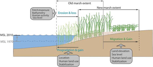
The overarching goal of this research is to examine how changes in natural and anthropogenic factors interact to affect tidal wetland resilience to sea-level rise and how variations in this response may affect marsh extent and distribution. Marshes change through three basic mechanisms: migration, erosion, and progradation (Figure 1). The rate at which these mechanisms drive change is determined by a variety of factors. Migration rates are not only tightly tied to sea-level rise but also respond to human activities, such as shoreline hardening. Erosion rates are driven by wave energy (a function of fetch, nearshore bathymetry, boating activity, and/or adjacent shoreline stabilization), which increases with sea-level rise due to increased nearshore water depths (Leatherman, Zhang, and Douglas 2000). Progradation relies on sediment supply, and so is affected by human land use and shoreline stabilization, which can reduce or exacerbate sediment supply (depending on the activity). We hypothesized that while the overall extent of marshes is declining, spatial variations in sea-level rise, erosion, sediment supply, and human development will result in spatially variable changes in specific marsh extents over the past 30 years.

Figure 1. Mechanistic drivers of marsh change. Mechanisms in gray boxes exacerbate or mitigate the effects of marsh change drivers.

Methods

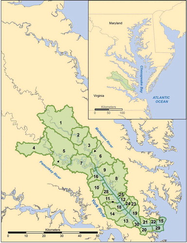
The York River estuary, Virginia, USA is the target site for this study (Figure 2). It is one of five major tributary systems in Chesapeake Bay and generally representative of conditions encountered throughout the Bay and similar estuaries (Reay and Moore 2009). The York River estuary is a brackish system approximately 64-km-long branching into two smaller tributaries: the Mattaponi and Pamunkey rivers at 55 km from the mouth of the estuary. It possesses a wide range of salinities from approximately 20 ppt near the mouth of the estuary to 0 ppt several kilometers upriver of the branch. The estuary has a primary turbidity maximum near the branching point and a secondary turbidity maximum approximately 30 km from the mouth of the estuary (Lin and Kuo 2001). Mean tidal range near the mouth of the York River is 0.7 m and increases to 1.1 m in the upper reaches of the Mattaponi River (Sisson et al. 1997) and the Pamunkey shows a similar trend. The estuary supports a wide range of habitats, including freshwater swamps, tidal freshwater marshes, and salt marshes, and the watershed is dominated by forested (61%) and agricultural (21%) land use, with developed areas mostly near the mouth of the estuary (Reay 2009). Subsidence varies along the length of the estuary, from approximately 2.8 mm/year at the mouth of the estuary to approximately 3.8 mm/year at the branching point (Eggleston and Pope 2013). Marsh cores along the main stem of the York River show top layer soils to be silt and clay with organic inclusions of Spartina alterniflora (Finkelstein and Hardaway 1988). Certain areas of the watershed have seen large increases in development since the 1970s, while other areas have had little change (Table A1). Coastal development has been greatest in the Gloucester Point and Yorktown areas (subwatersheds 19, 20, 21, and 30; personal observation, Hershner). Census data show the most population growth between 1970 and 2010 occurring in James City County, followed by Gloucester and York counties. The growth in James City County is misleading, since only a small portion of the locality is in the York River watershed and 2010 population densities show that those census tracts have very low population density (Appendix 2).

Figure 2. York River estuary subwatershed boundaries and numbers.

Inventory development

The TMI(CCRM, VIMS 1992) is a geospatial survey of all tidal marshes in Virginia, including their location, extent, and plant community; the survey has been done twice, approximately 30 years apart. The surveys involved digitization of marsh extents and locations from maps and aerial imagery. The digitization was field verified for all main stem marshes and most creek marshes. Field verification data collection in both surveys was conducted using a shallow-draft vessel driven close to shore along the entire shoreline of the York River estuary. Every marsh was compared to the digital coverage and marshes were added or altered where necessary. Changes to the dataset from verification were minimal. The addition of very narrow (>5 m width) fringe marshes, hidden on the aerial photography by overhanging trees, was the most common change in both time periods. Plant community data were used to delineate the upstream extent of tidal inundation and only tidal marshes were included in the inventories. Marshes were also categorized by their form (i.e., fringe, extensive, embayed, marsh island; Table 1 for category definitions).

Table 1. Marsh forms.

Forms	Diagram	Characteristics	Water edge:area	Typical wave exposure
Extensive (attached)		Large, flat marshes with extensive marsh channels; attached to land on one edge	Small (not including creek edges)	Frequently in high-exposure areas, unless riverine
Extensive (marsh island)		Large, flat marshes with extensive marsh channels; islands	Small (not including creek edges)	Frequently in high-exposure areas
Embayed		V-shaped marshes that form along the edges and tops of creeks; some marsh channels	Moderate	Frequently in sheltered area
Fringing		Long, narrow marshes that form along river and creek edges; few marsh channels	High	Found equally in high energy and sheltered areas

In the York River estuary, the original survey was digitized from USGS topographic maps that were originally mapped in the late 1950s to early 1960s. Field verification was done between 1974 and 1987 (depending on the county), making it difficult to assign a specific year to the data. The second survey, in the York River, was digitzed from 2009 aerial imagery (VBMP) and field verified in 2010.

Tidal marsh digitization

The original survey was digitized at 1:24,000 resolution with a reported horizontal accuracy of ±12.2 m. Topographic maps printed on stable-based mylar were placed on Numonics 2200 series digitizing tablets and marsh boundaries were hand digitized using precision cursors. Tablets were interfaced with SUN Unix workstations running the ESRI software ArcInfo®. Mylar maps were geo-registered on the tablet using a quality assurance digitizing standard of RMS = 0.002 in or better. Other program and computer-based standards were put in place to insure accuracy of the digital product, including a node snap tolerance (<0.05 in) and fuzzy tolerance (0.001 in = 1.0 m in Universal Transverse Mercator [UTM]), which are procedural standards that control digitizing accuracy and final product quality (Berman, Smithson, and Kenne 1993).

In the recent TMI survey, tidal marshes were digitized off digital high resolution (6 in) color infrared aerial photography collected in 2009 (VBMP) at 1:1000 resolution. Heads-up digitizing (capturing vector objects directly from the computer screen using a mouse or cursor) was performed to develop the boundary delineation for current wetland distribution. This method is considered more accurate than traditional tablet digitizing since the user can resolve more features using zoom functions. Photo interpretation techniques were used to identify wetland objects on the screen in ArcMap versions 9.3 and 10.0. Ancillary datasets including the VA Shoreline Inventory (Berman et al. 2013, 2014a, 2014b, 2014c) and National Wetlands Inventory (NWI) were used to help identify narrow fringe marshes masked by tree canopy or visual scale. When digitizing was complete, the file was smoothed to improve the cartographic quality. The smoothing algorithm used was PAEK (Polynomial Approximation with Exponential Kernal) using a smoothing tolerance of 5 m.

Quality control and assurance was by independent scientist review and during field work. During field observations, marsh boundaries were added or visually adjusted on rectified image base maps. Digital corrections were made in the lab when community composition data were added to the attribute files. Consistency in identifying and digitizing the marsh boundary was tested using repetitive sampling techniques. Six marshes of varying size and complexity were selected and each digitized three times. Each digitized area was compared to the mean; the average difference in calculation of area for each sample was ±0.0003 ac.

Dataset corrections

Examination of the old TMI against current elevation data (CoNED TBDEM 2016) showed that there were errors in the landward extent of some marshes, particularly the fringe marshes, leading to overestimation of marsh extent in the original survey. These errors were due to the resolution at which digitization occurred in the original survey and the fact that many fringing marshes were discovered during the field-verification whose exact widths were difficult to determine. To minimize these errors, marshes in the original survey were clipped to an elevation (1 m NAVD88) representing the theoretical maximum elevation of tidal wetlands in 1970. This correction removed 5988,795 m² of wetlands (8% of the total digitized wetland area) that were clearly digitized into upland areas. Results were verified against available aerial photos from the 1960s of the York River estuary.

Watershed characterization

High spatial variability in estuarine characteristics makes it difficult to see patterns in marsh change. Therefore, the York River estuary was divided into subwatersheds based on the broader designations of the NWBD (National Watershed Boundary Database 2008) and split into smaller subwatersheds, where needed, using elevation contours. This kept marshes which would reasonably be responding to similar land use and water-quality measures in a single subwatershed (e.g., creek marshes and main stem marshes that were immediately adjacent to the creek mouth, tending to extend further downriver than up), while still minimizing the variability in estuarine characteristics.

Subwatersheds were characterized by location and marsh form. Location of the subwatershed was measured as the distance from the mouth of the estuary, up the centerline of the estuary, to the center of each subwatershed, using the Measure tool in ESRI ArcMap (10.2). The continuous distances (km) were used for the analysis; however, for ease of discussion, marshes are referred to by three location groups with similar hydrodynamic characteristics in the “Results” and “Discussion” sections: lower estuary (high energy, <20 km from mouth), mid-estuary (moderate energy in main stem, low energy in creeks, >20 and <58 km from mouth), and upper/riverine (low energy, river-dominated, >58 and <64 km from mouth).

Land use and shoreline stabilization

Land use within a 1500-m buffer of the shoreline was obtained from the VGIN 1 m Land Cover dataset (released 2016, developed from 2013 to 2014 aerial photography). Land use was grouped into three categories based on similar landcover types: (1) developed (included landcovers: impervious [extracted], impervious [local datasets], turf grass, barren), (2) natural (included landcovers: forest, tree, scrub/shrub, NWI/other), and (3) agriculture (included landcovers: harvested/disturbed, pasture, cropland). Each category was summed by subwatershed and percent cover was calculated for each. Shoreline stabilization lengths were obtained from the shoreline inventory (Berman et al. 2013, 2014a, 2014b, 2014c). There are multiple categories of shoreline stabilization, but only bulkhead and riprap (“hardening” henceforth) were used since these structures disconnect the tidal marsh from the upland, reducing both function and the ability of the marsh to migrate (Bilkovic and Mitchell 2017). Length of hardening was summed by subwatershed.

Elevation

Low elevation areas adjacent to tidal marshes enhance tidal marsh migration. Areas with very low relief can allow migration to proceed at a pace equal to or greater than marsh erosion, leading to marsh expansion. To see the importance of elevation as a driver of marsh change, a metric of elevation (henceforth, % low) was developed. Elevation data were obtained from a seamless lidar-derived digital topographic and point-derived bathymetric elevation model (CoNED TBDEM 2016). Elevations below 1 m NAVD88 (tidal marsh elevations) were discarded due to concerns about the accuracy of elevations in salt marshes (Hladik and Alber 2012; Wang et al. 2009). Elevations above 3 m NAVD88 were also discarded since they represent lands which are unlikely to be marsh at any time between the start of the survey and 2100 (based on the high scenario projection of mean sea level; Sweet et al. 2017). Elevations between 1 and 3 m are transitional areas with the potential to become tidal marshes by 2100, therefore, critical habitat for marsh migration. Elevations between 1 and 3 m NAVD88 within a 1500-m buffer from the creek were extracted from the Digital elevation model (DEM). Within each subwatershed, the percent of land represented by this range in elevation (% low) was calculated for the extracted data.

Statistical analysis

All statistical analyses were done in JMP 10 (SAS). A recursive partition analysis using a decision tree was used to classify percent marsh change according to subwatershed characteristics: location of the watershed in the estuary, land use (% developed, % agriculture, % tural), marsh form (% fringing, % embayed, % extensive), shoreline hardening (m) along watershed shorelines, and elevation (% low). Recursive partitioning decision trees are a nonparametric, multivariate, classification, and regression tree-type analysis. Decision trees explain the variation in a response variable (in our case, % change in marsh) as a function of multiple explanatory variables can handle variables with nonlinear relationships and are not affected by monotonic transformations (De’ath and Fabricuis 2000). KFold validation (KFold = 10) was used to select the final model (JMP 10). This process reduces overfitting of the model; however, overfitting of the tree was unlikely given the low complexity of the resulting model (Olden et al. 2008). Splits in continuous data were made on the explanatory variable with the greatest LogWorth at each step in the tree. Automatic splitting was used, where splitting continues until the KFold validation r² exceeds the values that the next 10 splits would obtain (JMP 10).

For decision trees, correlations between independent variables can complicate the analysis. We performed a correlation analysis on our explanatory variables to elucidate potentially important variables not explicitly identified in the tree.

Results

Marsh change

Between the early 1970s and 2009, sea level rose approximately 20 cm in the York River estuary while concurrent overall marsh change was a loss of approximately 2187,000 m² or ~2.7% of marsh area from the original survey. Marsh change varied by subwatershed, with some watersheds showing an increase in marsh area while others showed losses (Table 2 and Figure 3).

Table 2. Summary by subwatershed.

Watershed	Location	Approximate distance (km)	Old TMI marsh extent (m^2)	New TMI marsh extent (m^2)	Percent age of change in marsh extent	Leaf group
1	Upper	83	3204,315	3296,848	2.89	1
2	Upper	74	1842,669	2046,628	11.07	1
3	Upper	58	5984,716	5957,608	−0.45	1
4	Upper	83	1398,541	1318,269	−5.74	1
5	Upper	74	6063,007	6022,791	−0.66	1
6	Upper	58	7669,161	7722,836	0.70	1
7	Upper	58	21,740,124	21,541,880	−0.91	1
8	Mid	40	9976,593	9904,033	−0.73	2
9	Mid	51	2733,013	2702,113	−1.13	2
10	Mid	45	1879,906	1889,505	0.51	3
11	Mid	34	2112,664	2025,131	−4.14	3
12	Mid	30	718,054	672,257	−6.38	3
13	Lower	19	1560,796	1672,170	7.14	3
14	Mid	24	2483,726	2317,941	−6.67	4
15	Lower	2	994,826	744,878	−25.12	2
16	Mid	51	2295,306	2041,473	−11.06	2
18	Mid	29	925,482	698,189	−24.56	4
19	Lower	18	2000,614	1466,219	−26.71	4
20	Lower	10	140,239	115,403	−17.71	4
21	Lower	10	150,813	116,243	−22.92	4
22	Lower	5	595,644	406,073	−31.83	4
23	Mid	23	815,024	706,616	−13.30	2
24	Mid	26	296,018	254,917	−13.88	2
25	Mid	3	303,942	302,270	−0.55	3
28	Mid	40	725,091	649,417	−10.44	3
29	Lower	4	1187,314	1013,941	−14.60	4
30	Lower	15	155,879	161,300	3.48	4

TMI: Tidal Marsh Inventory.

Figure 3. The percent change in marsh area by distance from the mouth of the estuary. The x and y coordinates indicate UTM eastings and northings. Numbered regions are subwatersheds used in the analysis. Negative values represent marsh loss, positive values represent marsh gain.

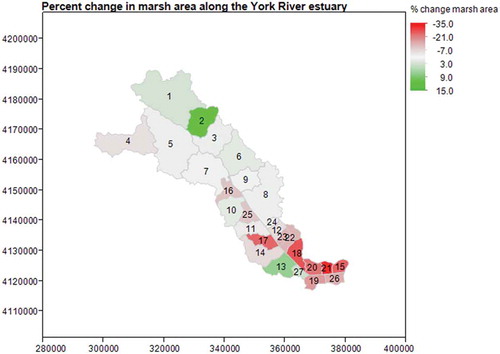
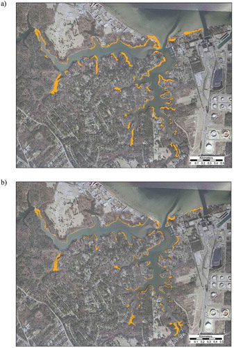
Examination of the marsh change and aerial photography from both time periods indicated that most of the marsh loss is due to edge erosion (reduction in marsh width), with minimal loss of linear marsh extent (reduction in marsh length or total loss). However, in subwatersheds 19 and 20 (which are predominantly fringing marsh systems that are developed with extensive shoreline stabilization), there is total loss of multiple marshes. This has resulted in both a loss of area and fragmentation of the marsh system (Figure 4).

Figure 4. Wormley Creek, York VA. Example of marsh fragmentation and loss due to shoreline stabilization. (a) Old TMI marsh distribution shown on an aerial photo from 2009. (b) New TMI marsh distribution shown on an aerial photo from 2009.

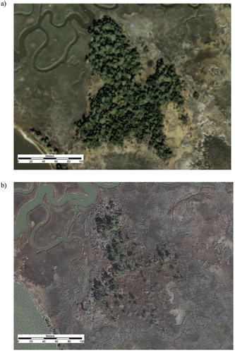
Examination of the marsh change and aerial photography from both time periods indicated that most of the marsh gain is due to landward migration, frequently into previously forested hummocks (Figure 5). A couple of subwatersheds in the upper/riverine section of the estuary showed slight marsh expansion through progradation.

Figure 5. Catlett Islands, Gloucester VA. Example of marsh migration into forested hummocks. (a) Aerial photo of the site from 1978, showing a large forested marsh hummock. (b) Aerial photo of the site from 2009, showing most of the hummock has converted to marsh.

Three subwatersheds in the mid-estuary (10, 13, and 30) showed gains in marsh area between the two surveys that were due to apparent upriver migration of tidal influence (i.e., in the original survey the marshes were nontidal, in the current survey they were tidal). In all cases, the expansion is linked to a barrier (bridge/culvert) and could have been caused by increased culvert size between the two surveys, allowing an expansion of the tidal influence. Unfortunately, the lack of tidal influence in the earlier time period could not be verified by aerial photography (vegetation was emergent in both time periods and the water line had not changed) and therefore the actual extent of tidal marsh gain in these sub-watersheds is uncertain.

Partition analysis

The partition analysis split the subwatersheds into four groups (Figure 6) based on (in order of split) development (split at 15%), approximate distance from the mouth of the estuary (split at 58 km), and percentage of embayed marshes (split at 61%). r² values increased with each split, and by the last split there were no likely candidates for splitting in any of the four groups.

Figure 6. Partition analysis results (a) AIC table, (b) tree diagram, and (c) map of leaf group position in the watershed.

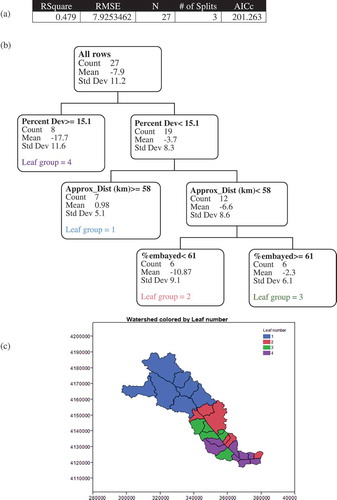
Development was the most important predictor of marsh change in the estuary, with areas of higher development having a higher percent loss of marsh. However, land use within a 1500-m buffer of the shoreline was predominantly natural (mean % natural land use = 75%), with only two subwatersheds having greater than 40% developed land (Appendix 1). Percentage of developed land use was somewhat negatively correlated with % natural land use (r² = −0.62); so, it could be considered that the tree is splitting on a balance between developed and natural lands within the subwatersheds, but the evidence for this is not strong. Although a few subwatersheds had high agricultural levels, it was never the dominant land use in a subwatershed and plays a small role overall in the estuary (mean % agriculture land use = 12%). It was only weakly correlated with % developed land use (r² = −0.30) and therefore is not a discriminant factor in the York River estuary. Interestingly, % developed lands were highly positively correlated with length of riprap and bulkhead (r² = 0.85) and % fringe marsh (r² = 0.77), suggesting these might be important predictors of marsh loss that were not identified in the decision tree. Shoreline hardening was highest in subwatersheds in the lower section of the estuary and minimal throughout the rest of the estuary. Three subwatersheds on the southside of the mid-estuary (10, 13, and 30) had no shoreline hardening at all. These are the same subwatersheds where there appeared to be marsh gain through the conversion of upriver migration of tidal influence.

In areas of low development, the distance upstream (a proxy for fetch) was the most important factor predicting marsh change. In low development watersheds located in the lower and mid-estuary, there was marsh loss on average, while in the upper estuary there was an average small increase in marsh acreage. Distance upstream was positively correlated with % agriculture land use (r² = 0.63) and negatively correlated with % developed land use (r² = −0.59) and % low (r² = −0.53). All other correlations were weak (r² < 0.40).

Land elevation within a 1500-m buffer of the shoreline showed a general pattern of lower elevations behind the marshes in the low estuary, with higher elevations on the south side of the river and in the mid-estuary and upper/riverine sections on both sides of the river (Appendix 1). The analysis does not provide strong evidence for our expectation that marsh gains would be highest where there are the most opportunities for landward migration (highest % low). However, (1) there were gains in some of the low elevation-backed marshes, they were just outweighed by the losses and (2) the high elevation lands on the south side of the estuary include a number of eroding bluffs (Berman et al. 2013, 2014b) which may contribute sediment supply essential for marsh persistence.

In areas of low development in the lower and mid-estuary, the % embayed marsh was the most important factor predicting marsh change. There was more marsh loss in areas with less than 61% embayed marsh. The % embayed marsh is strongly negatively correlated with % extensive marsh (r² = −0.89) but weakly (r² < 0.40) correlated with all other explanatory variables. Extensive marshes might be important predictors of marsh loss, in this subset of marshes, which were not identified in the decision tree. In general, in this subset of marshes, extensive marshes are found on the main stem of the estuary, and subject to higher energy, while embayed marshes are found in sheltered tributary creeks.

Discussion

Marsh change along the York River estuary is highly variable and that variability is not primarily explained by differences in erosion rates and migration potential, as would be expected under rising sea levels. Development and marsh form interact with location in the estuary, a surrogate for erosion potential, to modify the marsh response to sea-level rise. Although the extent of marsh change groups into four categories, there is variability in response even within those categories. This variability calls into question the current practices of evaluating regional marsh change with studies of only one or a few marshes and/or studies limited to only extensive marshes.

Extending the marsh change estimates in one marsh or creek system to an estuarine scale requires careful understanding of the spatial variability of the drivers of change and the magnitude of their importance in each setting. Considering only net overall change in estuarine marsh extent does not adequately represent the potential impact to the resource. In this study, marsh change was highly variable across subwatersheds, ranging between a 32% loss and an 11% gain in marsh extent. The importance of the marsh loss to overall estuarine function may depend on the location and type of marsh lost. Loss was focused in the brackish part of the estuary, compared to the more stable oligohaline areas. In addition, much of the marsh loss was in fringing marshes which constitute a small part of the total estuarine acreage, but a disproportionately large part of the ecosystem service capacity (Bilkovic et al. 2017b; Bilkovic and Mitchell 2017; Beck et al. 2017).

Spatial differences in marsh response

Developed land use was the most important predictor of marsh loss. Subwatersheds with high development (Leaf group 4) tend to have extensive creeks edged with fringe marshes. They also tend to have stabilized shorelines, heavy boat traffic, and lawns that extend to the water. These three factors may explain the link between development and marsh loss. Boat wakes have been shown to negatively impact shoreline stability in salt marshes (Castillo et al. 2000; Bilkovic et al. 2017a) and shoreline structures (bulkheads in particular) reflect wave energy, exacerbating erosion. Another link between human development and marsh loss, which might be explained by these patterns, is eutrophication due to fertilization (Deegan et al. 2012). Although it is not clear which of these factors is responsible for the loss in developed creeks, creek systems with lower development (found in Leaf group 3) with lots of natural lands surrounding them and relatively little shoreline stabilization had lower marsh loss.

In the lower development areas, distance up the estuary (a proxy for wave energy) becomes an important explanatory variable. Wind-driven wave energy is considered the predominant driver of marsh erosion on coastal shorelines (Schwimmer 2001) which supports finding in this study that marsh loss generally decreased with distance from the mouth of the estuary (Figure 3). However, it was not the predominant driver, since within this general trend there is still significant variability among subwatersheds in the same section of the estuary. The greater importance of development in explaining marsh change suggests that human influences on marsh persistence may equal or exceed physical influences.

However, wind-wave energy is only one of the physical influences of importance. Local sea-level rise variations could be important in explaining marsh change but the magnitude of variation in local sea-level rise is impossible to determine with existing data. Sea-level rise variations could affect both marsh loss and gain processes. As sea-level rises, it increases the depth of inundation on the marsh surface, which triggers responses in vegetation (Morris et al. 2002), sediment accumulation (Kirwan and Murray 2007), and erosion (Mariotti and Fagherazzi 2010). These responses are specific to plant species and marsh position (and may be related to associated fauna, such as ribbed mussel [Guekensia demissa] presence), leading to spatial variability in marsh response to sea-level rise. In addition, subsidence can vary on small spatial scales (Cahoon 2015) causing marshes in neighboring subwatersheds to experience different rates of relative sea-level rise. High rates of sea-level rise can lead to marsh drowning, but in areas with sufficient sediment supply and low elevation adjacent lands, it can lead to marsh expansion. In the York River estuary, the highest known rate of subsidence (Eggleston and Pope 2013) is found in the group of subwatersheds (subwatersheds 6 and 7) located at the estuarine turbidity maximum, suggesting ample sediment supply. Overall, they are showing little change (<1% change) in marsh extent, suggesting that the sediment supply may be compensating for the increased rate of sea-level rise. However, their low elevation adjacent lands suitable for marsh migration are constrained. With continued acceleration in sea-level rise rates, this area may be less resilient than it currently appears to be.

As sea-level rises, riparian land elevation is the dominant factor controlling marsh migration potential, although it is moderated by development (which is the most important factor controlling marsh change in the partitioning analysis). Areas with low elevation lands immediately adjacent to wetlands show signs of marsh gain through migration, with marsh gain in the lower estuary primarily seen in extensive marshes as migration into interior forested hummocks (Figure 5), and along the river shoreline as migration into low-lying riparian uplands. Models of the Chesapeake Bay region suggest that the conversion of forest hummocks to marsh will continue with sea-level rise but represents only a small area of potential future gain (http://www.slammview.org/). Subwatersheds 21 and 22 are areas which would be expected to show marsh gain through migration due to their low riparian elevations. Instead, they have had a loss in marsh extent of 13% and 31%, respectively. The shorelines in these subwatersheds are heavily stabilized, blocking upland migration (Figure 4) and potentially impacting sediment availability by trapping sediment landward of the bulkhead (Douglass and Pickel 1999; Griggs 2005).

It is unlikely that sea-level rise rates vary more than a couple mm/year along the York River estuary, based on available subsidence rates (Eggleston and Pope 2013) and the unimportance of marsh expansion through progradation. Progradation, the chanelward growth of marshes into previously unvegetated intertidal zone, is controlled by the balance between nearshore sedimentation and sea-level rise (Schwimmer and Pizzuto 2000), and it is typically favored by low rates of sea-level rise (Mariotti and Fagherazzi 2010). Examples of progradation are only seen in the upper/riverine subwatersheds of the York River system, above the turbidity maximums (e.g., subwatershed 2). Even in these areas, it is a minor process, despite the presence of higher total suspended solids (TSS) (Reay 2009) and eroding bluffs which should provide ample sediment supply. Sediment supply is the counterpoint to sea-level rise, enhancing marsh persistence. Without sufficient sediment supply, marshes can begin to pond, leading to fragmentation and permanent loss (Mariotti 2016) while ample supply leads to marsh accretion and expansion. Published values for the York River estuary (Reay 2009) suggest that TSS are most likely to contribute to marsh gain and persistence around the two turbidity maximums. The primary turbidity maximum is found in subwatersheds 6, 7, 9, and 16. But marsh extent change was minimal in these areas and progradation did not occur. Subwatershed 16 actually shows losses likely due to marsh fragmentation. Despite the low levels of development and shoreline stabilization in these subwatersheds, sediment supply is apparently still inadequate to counter the local rates of sea-level rise.

Comparison of historic and modern marsh extents

Comparisons of historic and modern marsh extents should always be approached with caution. Comparison errors are unavoidable but can be minimized with good digitization and verification processes, allowing accurate determination of past shoreline changes (Crowell, Leatherman, and Buckley 1991). Errors stem from the precision (scale) of the aerial photography used in the marsh delineation and the digitizing technology. In our case, the old aerial photography was the limiting driver of the error, but it was mitigated by the field verification process. Using aerial photography alone (at a scale of 1:24,000) would preclude the inclusion of narrow (<5 m wide) marshes in the original survey, and potentially leading to an overestimation of marsh gain. However, these marshes were added following the field surveys, improving the accuracy of the surveys.

In addition to the error due to technological limitations, there is an undefinable interpretation error, both during the digitizing and the field verification. Both the wetland/upland boundary and the water/wetland boundary are subject to this error (Anderson and Roos 1991; McCrain 1991). The water/wetland boundary is defined as mean high water, but aerial photography is seldom tidally coordinated, leaving room for interpretation by the digitizer. We minimized this error through constant definitions of mean high water signals (e.g., edge of vegetation in S. alterniflora marshes) and verification of the digitization (each digitization is verified by two independent reviewers). The wetland/upland boundary can be subject to interpretation, particularly where mowed lawns intersect with marshes. This error was minimized by training on signals of waterlogged soils, the verification processes, and the use of a lidar-based digital elevation model to define elevations above the tidal extent.

Consequences of marsh change on ecosystem health

Ecological concerns with the observed shifts in marsh extent include both loss and redistribution of ecological services provided by marshes, particularly water quality and habitat functions. For both of these functions, location is often as important, if not more important, than total amount of marsh. Fragmentation and relocation enhance the potential for the disconnection of marsh service capacity from landscape-based needs and opportunities.

Percent marsh losses were heaviest in fringing marsh systems, which are ecologically important due to their high edge:area ratio. Despite their small acreages, fringe marshes have been found to have similar wave attenuation, nutrient removal, sediment accretion, and habitat values compared to extensive marshes (Bilkovic et al. 2016). In the original survey, fringe marshes were nearly continuous along the shoreline, while in the current survey, they have become fragmented in many creek systems, particularly those with high development and shoreline stabilization structures. Fragmentation threatens marsh resilience under sea-level rise, as there is more exposure for erosion. In addition, habitat fragmentation in terrestrial and estuarine systems has been linked with shifts in biodiversity, loss of habitat-specific sensitive or functionally important species, and isolation of populations when connectivity is diminished (Kareiva and Wennergren 1995; Fahrig 2003; Thrush et al. 2008; Collinge 2009).

All types of marshes are efficient at removing sediments (Friedrichs and Perry 2001) and nutrients (Deegan et al. 2007) from the tidal waters, and nutrients from groundwater (Tobias et al. 2001), but fringing marshes may be particularly important to the nutrient balance in estuaries due to their role in groundwater nutrient removal (Beck et al. 2017) and their near continuous presence along undisturbed shorelines. In the Chesapeake Bay, groundwater discharge of nutrients may be as high as 30% of surface inputs (Libelo, MacIntyre, and Johnson 1991), potentially making fringe marshes a critical mediator of estuary water quality. The fragmentation of fringe marshes seen in this study along developed shorelines likely reduces the provision of nutrient removal services in affected watersheds; however, this is a topic that requires more study.

The loss of marsh in the developed creek systems (>15% developed) suggests that they may be approaching or even have crossed an ecological threshold (breakpoints at which a system or community notably responds, perhaps irreversibly to a disturbance). Ecological thresholds studies suggest that the relationship between development and ecological function is not a gradual, linear relationship and that alarmingly low levels of development (between 10% and 25%) can dramatically diminish a multitude of system functions (e.g., Wang, Lyons, and Kanehl 1997; Limburg and Schmidt 1990; Paul and Meyer 2001; DeLuca et al. 2004; Brooks et al. 2006; King et al. 2005; Bilkovic et al. 2006; Lussier et al. 2006).

Marsh losses by area were highest in extensive marshes, particularly marsh islands, which are important habitats for avian species (Wilson, Watts, and Brinker 2007). Both fringing marshes and marsh islands have limited potential for migration in this estuary, so loss to erosion may not be counterbalanced in the long term (e.g., Schile et al. 2014). Embayed marshes appear particularly resilient to loss over time, with small embayed marshes persisting at the tops of creeks where long extents of fringe marsh have been lost. Migration of tidal marshes into upland habitats is not a dominant process in the estuary but will mitigate some of the wetlands loss. These new tidal marshes should provide similar habitat and water-quality functions. They do not provide the same carbon storage function because wetland soils take many years to develop (Craft et al. 2003). Migration of tidal marshes into previously nontidal wetlands (as seen in some of the subwatersheds) may result in some changes in function (nontidal wetlands provide different types of habitat and have different nutrient cycling pathways) but should have a net neutral impact to water quality.

Conclusions

Within a single estuary, marsh change over time shows high spatial heterogeneity related to the variability in the importance of and interactions between multiple drivers. Erosion rates, migration opportunities, and the rate of sea-level rise all affect marsh persistence. Importantly, human actions are also critical, and frequently less predictable, determinants of how marshes respond through time.

Improving our understanding of marsh change requires examination of change on ecosystem scales. Despite the use of an entire estuarine system in this study, extension of results to characterize an even larger system (e.g., Chesapeake Bay) is probably inappropriate. Forecasts of ecosystem change based on small scale studies often lead to inaccurate or unsubstantiated conclusions. The processes leading to change are spatially variable and not always predictable.

There are, however, some lessons that can be taken from this study:

1. Human shoreline use (e.g., development, shoreline hardening, boating activity) can dominate physical processes and alter the marsh response to sea-level rise.

2. Defining sediment availability for a given marsh may not be sufficient to determine its potential for expansion or persistence under sea-level rise.

3. Marsh response varies by form as well as setting, and ecologically important fringe marshes may be particularly vulnerable.

Understanding past changes in marsh extent are critical for improved prediction of future change under accelerating sea-level rise. Knowing which marshes are most vulnerable allows for the prioritization of restoration and conservation efforts, minimizing future impacts to estuarine systems.

Acknowledgments

We would like to thank all the present and past scientists who contributed to the York River tidal marsh inventories, particularly: Marcia Berman, Harry Berquist, Sharon Killeen, Julie Bradshaw, Karen Duhring, Dave Stanhope, and Kory Angstadt. We would also like to thank the anonymous reviewers whose comments helped improve the manuscript. This study was supported by Environmental Protection Agency Award: [Grant Numbers CD96329601-1 and CD-97386001-0]. This paper is Contribution No. 3673 of the Virginia Institute of Marine Science, College of William & Mary.

Disclosure statement

No potential conflict of interest was reported by the authors.

Additional information

Funding

This study was supported by Environmental Protection Agency Award: [Grant Numbers CD96329601-1 and CD-97386001-0].

Appendices

Appendix 1

Table A1. Subwatershed characteristics.

Watershed	Percentage of developed land use	Percentage of agriculture land use	Percentage of natural land use	Percentage of fringing marshes	Percentage of extensive marshes	Percentage of embayed marshes	Percentage of low elevation land	Riprap and bulkhead length (m)
1	6	30	65	9	78	13	6	1545
2	4	12	84	7	65	27	5	512
3	4	20	77	0	89	10	9	1210
4	4	44	51	5	21	74	6	521
5	4	23	73	11	68	21	7	708
6	11	18	71	1	75	24	16	942
7	8	16	76	1	92	7	11	3068
8	5	13	82	1	71	29	24	2882
9	12	11	77	2	76	22	33	1396
10	2	4	94	6	0	94	7	0
11	9	3	88	2	37	61	7	627
12	6	17	77	1	10	88	11	2140
13	13	1	86	11	24	65	4	0
14	16	1	83	3	74	23	7	759
15	8	0	92	3	97	0	100	630
16	8	10	82	5	65	30	17	1316
18	15	2	83	13	0	87	9	1433
19	29	16	54	10	75	15	7	4082
20	42	6	52	70	0	30	16	8581
21	50	6	45	53	2	45	54	13,852
22	19	11	70	26	19	55	100	2868
23	7	22	71	3	45	53	8	890
24	12	28	60	37	4	59	6	2326
25	11	14	74	1	0	99	4	698
28	5	2	93	21	0	79	6	787
29	17	0	82	2	98	0	100	1576
30	19	3	77	15	0	85	8	0

Appendix 2

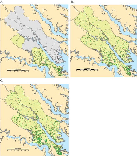
Maps showing population distribution in York River estuary localities from 1970 to 2010. Boundaries are census tracts. Green dot = 100 people. Gray localities do not have census tract data available in 1970. Figure A is 1970, figure B is 1990, and figure C is 2010. Data are from the national census and were statistically distributed to 2010 census tract boundaries by Geolytics.

References

- Anderson, J., and M. Roos. 1991. “Using Digital Scanned Aerial Photography for Wetlands Delineation.” Earth and Atmospheric Remote Sensing, SPIE 1492: 1–16.
- Barbier, E. B., S. D. Hacker, C. Kennedy, E. W. Koch, A. C. Stier, and B. R. Silliman. 2011. “The Value of Estuarine and Coastal Ecosystem Services.” Ecological Monographs 81: 169–193. doi:10.1890/10-1510.1.
- Beck, A., R. M. Chambers, M. M. Mitchell, and D. M. Bilkovic. 2017. “Evaluation of Living Shoreline Marshes as a Tool for Reducing Nitrogen Pollution in Coastal System.” In Living Shorelines: The Science and Management of Nature-Based Coastal Protection, edited by D. M. Bilkovic, M. Mitchell, J. Toft, and M. La Peyre, 271–292, Boca Raton, FL: Taylor & Francis Group and CRC Press; CRC Press Marine Science Series.
- Beckett, L. H., A. H. Baldwin, and M. S. Kearney. 2016. “Tidal Marshes across a Chesapeake Bay Subestuary are Not Keeping up with Sea-Level Rise.” PloS One 11 (7): e0159753. doi:10.1371/journal.pone.0159753.
- Berman, M. R., J. B. Smithson, and A. K. Kenne. 1993. Guidelines for Quality Assurance and Quality Control, Comprehensive Coastal Inventory Program, Center for Coastal Management and Policy, 18. Gloucester Point, VA: Virginia Institute of Marine Science, College of William and Mary.
- Berman, M. R., K. Nunez, S. Killeen, T. Rudnicky, C. H. Hershner, K. Angstadt, D. Stanhope, D. Weiss, K. Duhring, and C. Tombleson. 2013. “York County - Shoreline Inventory Report: Methods and Guidelines.” SRAMSOE No. 439, Comprehensive Coastal Inventory Program, 23062. Gloucester Point, VA: Virginia Institute of Marine Science, College of William and Mary.
- Berman, M. R., K. Nunez, S. Killeen, T. Rudnicky, J. Bradshaw, K. Duhring, D. Stanhope, et al. 2014c. “Gloucester County, Virginia - Shoreline Inventory Report: Methods and Guidelines.” SRAMSOE No.441, Comprehensive Coastal Inventory Program, 23062. Gloucester Point, VI: Virginia Institute of Marine Science, College of William and Mary.
- Berman, M. R., K. Nunez, S. Killeen, T. Rudnicky, J. Bradshaw, K. Duhring, K. Angstadt, A. Procopi, D. Weiss, and C. H. Hershner. 2014a. “James City County and City of Williamsburg, Virginia - Shoreline Inventory Report: Methods and Guidelines.” SRAMSOE No. 440, Comprehensive Coastal Inventory Program, 23062. Gloucester Point, VA: Virginia Institute of Marine Science, College of William and Mary.
- Berman, M. R., K. Nunez, S. Killeen, T. Rudnicky, J. Bradshaw, K. Duhring, K. Angstadt, A. Procopi, D. Weiss, and C. H. Hershner. 2014b. “James City County and City of Williamsburg, Virginia - Shoreline Inventory Report: Methods and Guidelines.” In SRAMSOE No. 440, Comprehensive Coastal Inventory Program, 23062. Gloucester Point, VA: Virginia Institute of Marine Science, College of William and Mary.
- Bilkovic, D., M. Mitchell, J. Davis, E. Andrews, A. King, P. Mason, J. Herman, N. Tahvildari, and J. Davis. 2017a. “Review of Boat Wake Wave Impacts on Shoreline Erosion and Potential Solutions for the Chesapeake Bay.” STAC Publication Number 17-002, 68. Edgewater, MD: Chesapeake Bay Program, STAC.
- Bilkovic, D. M., M. Mitchell, P. Mason, and K. Duhring. 2016. “The Role of Living Shorelines as Estuarine Habitat Conservation Strategies.” Coastal Management 44 (3): 161–174. doi:10.1080/08920753.2016.1160201.
- Bilkovic, D. M., M. Roggero, C. H. Hershner, and K. H. Havens. 2006. “Influence of Land Use on Macrobenthic Communities in Nearshore Estuarine Habitats.” Estuaries and Coasts 29 (6): 1185–1195. doi:10.1007/BF02781819.
- Bilkovic, D. M., and M. M. Mitchell. 2017. “Designing Living Shoreline Salt Marsh Ecosystems to Promote Coastal Resilience.” In Living Shorelines: The Science and Management of Nature-Based Coastal Protection, edited by D. M. Bilkovic, M. Mitchell, J. Toft, and M. La Peyre, 293–316, Boca Raton, FL: Taylor & Francis Group and CRC Press; CRC Press Marine Science Series.
- Bilkovic, D. M., M. M. Mitchell, R. E. Isdell, M. Schliep, and A. R. Smyth. 2017b. “Mutualism between Ribbed Mussels and Cordgrass Enhances Salt Marsh Nitrogen Removal.” Ecosphere 8 (4): e01795. doi:10.1002/ecs2.1795.
- Boon, J. D. 2012. “Evidence of Sea-Level Acceleration at US and Canadian Tide Stations, Atlantic Coast, North America.” Journal of Coastal Research 285 (6): 1437–1445. doi:10.2112/JCOASTRES-D-12-00102.1.
- Boon, J. D., and M. Mitchell. 2015. “Nonlinear Change in Sea-Level Observed at North American Tide Stations.” Journal of Coastal Research 316 (6): 1295–1305. doi:10.2112/JCOASTRES-D-15-00041.1.
- Bridgham, S. D., J. P. Megonigal, J. K. Keller, N. B. Bliss, and C. Trettin. 2006. “The Carbon Balance of North American Wetlands.” Wetlands 26 (4): 889–916. doi:10.1672/0277-5212(2006)26[889:TCBONA]2.0.CO;2.
- Brooks, R. P., D. H. Wardrop, K. W. Thornton, D. Whigham, C. Hershner, M. M. Brinson, and J. S. Shortle, eds. 2006. “Integration of Ecological and Socioeconomic Indicators for Estuaries and Watersheds of the Atlantic Slope.” In Final Report to U.S. Environmental Protection Agency STAR Program, Agreement R-82868401. Prepared by the Atlantic Slope Consortium, Report. 96 pp.+ attachments (CD). Washington, DC.
- Bruno, J. F. 2000. “Facilitation of Cobble Beach Plant Communities through Habitat Modification by Spartina Alterniflora.” Ecology 81 (5): 1179–1192. doi:10.1890/0012-9658(2000)081[1179:FOCBPC]2.0.CO;2.
- Cahoon, D. R. 2015. “Estimating Relative Sea-Level Rise and Submergence Potential at a Coastal Wetland.” Estuaries and Coasts 38 (3): 1077–1084. doi:10.1007/s12237-014-9872-8.
- Castillo, J. M., C. J. Luque, E. M. Castellanos, and M. E. Figueroa. 2000. “Causes and Consequences of Salt-Marsh Erosion in an Atlantic Estuary in SW Spain.” Journal of Coastal Conservations 6: 89–96. doi:10.1007/BF02730472.
- Center for Coastal Resources Management (CCRM), Digital Tidal Marsh Inventory Series. 1992. Comprehensive Coastal Inventory Program, 23062. Gloucester Point, VA: Virginia Institute of Marine Science, College of William and Mary.
- Chmura, G. L. 2013. “What Do We Need to Assess the Sustainability of the Tidal Salt Marsh Carbon Sink?” Ocean & Coastal Management 83: 25–31. doi:10.1016/j.ocecoaman.2011.09.006.
- Chmura, G. L., S. C. Anisfeld, D. R. Cahoon, and J. C. Lynch. 2003. “Global Carbon Sequestration in Tidal, Saline Wetland Soils.” Global Biogeochemical Cycles 17 (4). doi:10.1029/2002GB001917.
- Collinge, S. K. 2009. Ecology of Fragmented Landscapes, 360. Baltimore, MD: Johns Hopkins University Press.
- CoNED TBDEM. 2016 https://topotools.cr.usgs.gov/coned/chesapeake_bay.php
- Coverdale, T. C., C. P. Brisson, E. W. Young, S. F. Yin, J. P. Donnelly, and M. D. Bertness. 2014. “Indirect Human Impacts Reverse Centuries of Carbon Sequestration and Salt Marsh Accretion.” PLoS One 9 (3): e93296. doi:10.1371/journal.pone.0093296.
- Craft, C., P. Megonigal, S. Broome, J. Stevenson, R. Freese, J. Cornell, L. Zheng, and J. Sacco. 2003. “The Pace of Ecosystem Development of Constructed Spartina Alterniflora Marshes.” Ecological Applications 13 (5): 1417–1432. doi:10.1890/02-5086.
- Crowell, M., S. P. Leatherman, and M. K. Buckley. 1991. “Historical Shoreline Change: Error Analysis and Mapping Accuracy.” Journal of Coastal Research 7 (3): 839–852.
- De’ath, G. and Fabricius, K.E., 2000. Classification and Regression Trees: A Powerful yet Simple Technique for Ecological Data Analysis. Ecology 81 (11), 3178–3192.
- Deegan, L., J. Bowen, D. Drake, J. Fleeger, C. Friedrichs, K. Galvan, J. Hobbie, et al. 2007. “Susceptibility of Salt Marshes to Nutrient Enrichment and Predator Removal.” Ecological Applications 17 (5): S42–S63. doi:10.1890/06-0452.1.
- Deegan, L. A., D. S. Johnson, R. S. Warren, B. J. Peterson, J. W. Fleeger, S. Fagherazzi, and W. M. Wollheim. 2012. “Coastal Eutrophication as a Driver of Salt Marsh Loss.” Nature 490 (7420): 388–392. doi:10.1038/nature11533.
- DeLuca, W. V., C. E. Studds, L. L. Rockwood, and P. P. Marra. 2004. “Influence of Land Us on the Integrity of Marsh Bird Communities of the Chesapeake Bay, USA.” Wetlands 24: 837–847. doi:10.1672/0277-5212(2004)024[0837:IOLUOT]2.0.CO;2.
- Douglass, S. L., and B. H. Pickel. 1999. “The Tide Doesn’t Go Out Anymore”—The Effect of Bulkheads on Urban Bay Shorelines. University of South Alabama, Civil Engineering and Marine Sciences Departments, Mobile. Accessed January 25 2006. http://www.southalabama.edu/cesrp/Tide.htm
- Eggleston, J., and J. Pope. 2013. “Land Subsidence and Relative Sea-Level Rise in the Southern Chesapeake Bay Region: U.S.” Geological Survey Circular 1392: 30. doi:10.3133/cir1392.
- Ezer, T. 2013. “Sea Level Rise, Spatially Uneven and Temporally Unsteady: Why the US East Coast, the Global Tide Gauge Record, and the Global Altimeter Data Show Different Trends.” Geophysical Research Letters 40 (20): 5439–5444. doi:10.1002/2013GL057952.
- Ezer, T., and L. P. Atkinson. 2015. “Sea Level Rise in Virginia – Causes, Effects and Response.” Virginia Journal of Science 66 (3): 355–369.
- Fahrig, L. 2003. “Effects of Habitat Fragmentation on Biodiversity.” Annual Review of Ecology Evolution and Systematics 34 (1): 487–515. doi:10.1146/annurev.ecolsys.34.011802.132419.
- Finkelstein, K., and C. S. Hardaway. 1988. “Late Holocene Sedimentation and Erosion of Estuarine Fringing Marshes, York River, Virginia.” Journal of Coastal Research 4 (3): 447–456.
- Friedrichs, C. T., and J. E. Perry. 2001. “Tidal Salt Marsh Morphodynamics: A Synthesis.” Journal of Coastal Research 27: 7–37.
- Griggs, G. B. 2005. “The Impacts of Coastal Armoring.” Shore Beach 73 (1): 13–22.
- Hladik, C., and M. Alber. 2012. “Accuracy Assessment and Correction of a LIDAR-Derived Salt Marsh Digital Elevation Model.” Remote Sensing of Environment 121: 224–235. doi:10.1016/j.rse.2012.01.018.
- Kareiva, P., and U. Wennergren. 1995. “Connecting Landscape Patterns to Ecosystem and Population Processes.” Nature 373: 299–302. doi:10.1038/373299a0.
- Kennish, M. J. 2001. “Coastal Salt Marsh Systems in the US: A Review of Anthropogenic Impacts.” Journal of Coastal Research 17 (3): 731–748.
- King, R. S., M. E. Baker, D. F. Whigham, D. E. Weller, T. E. Jordan, P. F. Kazyak, and M. K. Hurd. 2005. “Spatial Considerations for Linking Watershed Land Cover to Ecological Indicators in Streams.” Ecological Applications 15 (1): 137–153. doi:10.1890/04-0481.
- Kirwan, M. L., and A. B. Murray. 2007. “A Coupled Geomorphic and Ecological Model of Tidal Marsh Evolution.” Proceedings of the National Academy of Sciences 104 (15): 6118–6122. doi:10.1073/pnas.0700958104.
- Kirwan, M. L., D. C. Walters, W. G. Reay, and J. A. Carr. 2016. “Sea Level Driven Marsh Expansion in a Coupled Model of Marsh Erosion and Migration.” Geophysical Research Letters 43 (9): 4366–4373. doi:10.1002/2016GL068507.
- Leatherman, S. P., K. Zhang, and B. C. Douglas. 2000. “Sea Level Rise Shown to Drive Coastal Erosion.” Eos, Transactions American Geophysical Union 81 (6): 55–57. doi:10.1029/00EO00034.
- Libelo, L., W. G. MacIntyre, and G. H. Johnson. 1991. “Groundwater Nutrient Discharge to the Chesapeake Bay: Effects of Nearshore Land Use Practices.” In New Perspectives in the Chesapeake Bay System: A Research and Management Partnership, edited by J. A. Mihursky and A. Chaney, 4–6. 137 vols. Edgewater, MD: Chesapeake Research Consortium. Pub.
- Limburg, K. E., and R. E. Schmidt. 1990. “Patterns of Fish Spawning in Hudson River Tributaries: Response to an Urban Gradient?” Ecology 71: 1238–1245. doi:10.2307/1938260.
- Lin, J., and A. Kuo. 2001. “Secondary Turbidity Maximum in a Partially Mixed Microtidal Estuary.” Estuaries 24: 707–720. doi:10.2307/1352879.
- Lussier, S. M., R. W. Enser, S. N. Dasilva, and M. Charpentier. 2006. “Effects of Habitat Disturbance from Residential Development on Breeding Bird Communities in Riparian Corridors.” Environmental Management 38 (3): 504–521. doi:10.1007/s00267-005-0088-3.
- Mariotti, G. 2016. “Revisiting Salt Marsh Resilience to Sea Level Rise: Are Ponds Responsible for Permanent Land Loss?” Journal of Geophysical Research: Earth Surface 121 (7): 1391–1407.
- Mariotti, G., and S. Fagherazzi. 2010. “A Numerical Model for the Coupled Long-Term Evolution of Salt Marshes and Tidal Flats.” Journal of Geophysical Research 115: F01004. doi:10.1029/2009JF001326.
- McCrain, G. R. 1991. “Highways and Pocosins in North Carolina: An Overview.” Wetlands 11: 481–487. doi:10.1007/BF03160763.
- Minello, T. J., L. P. Rozas, and R. Baker. 2012. “Geographic Variability in Salt Marsh Flooding Patterns May Affect Nursery Value for Fishery Species.” Estuaries and Coasts 35 (2): 501–514. doi:10.1007/s12237-011-9463-x.
- Morris, J. T., D. C. Barber, J. C. Callaway, R. Chambers, S. C. Hagen, C. S. Hopkinson, B. J. Johnson, et al. 2016. “Contributions of Organic and Inorganic Matter to Sediment Volume and Accretion in Tidal Wetlands at Steady State.” Earth’s Future 4 (4): 110–121. doi:10.1002/eft2.2016.4.issue-4.
- Morris, J. T., P. V. Sundareshwar, C. T. Nietch, B. Kjerfve, and D. R. Cahoon. 2002. “Responses of Coastal Wetlands to Rising Sea Level.” Ecology 83 (10): 2869–2877. doi:10.1890/0012-9658(2002)083[2869:ROCWTR]2.0.CO;2.
- National Watershed Boundary Database. 2008. https://nhd.usgs.gov/wbd.html
- Olden, J.D., J.J. Lawler, and N.L. Poff. 2008. “Machine Learning Methods Without Tears: A Primer for Ecologists.” The Quarterly Review of Biology 83 (2): 171–193. doi:10.1086/587826.
- Paul, M. J., and J. L. Meyer. 2001. “Streams in the Urban Landscape.” Annual Review of Ecology and Systematics 32: 333–365. doi:10.1146/annurev.ecolsys.32.081501.114040.
- Reay, W. G. 2009. “Water Quality within the York River Estuary.” Journal of Coastal Research 57: 23–39. doi:10.2112/1551-5036-57.sp1.23.
- Reay, W. G., and K. A. Moore. 2009. “Introduction to the Chesapeake Bay National Estuarine Research Reserve in Virginia.” Journal of Coastal Research 57: 1–9. Special Issue. doi:10.2112/1551-5036-57.sp1.1.
- Sallenger Jr., A. H., K. S. Doran, and P. A. Howd. 2012. “Hotspot of Accelerated Sea-Level Rise on the Atlantic Coast of North America.” Nature Climate Change 2 (12): 884–888. doi:10.1038/nclimate1597.
- Schile, L. M., J. C. Callaway, J. T. Morris, D. Stralberg, V. T. Parker, and M. Kelly. 2014. “Modeling Tidal Marsh Distribution with Sea-Level Rise: Evaluating the Role of Vegetation, Sediment, and Upland Habitat in Marsh Resiliency.” PLoS One 9 (2): e88760. doi:10.1371/journal.pone.0088760.
- Schwimmer, R. A., and J. E. Pizzuto. 2000. “A Model for the Evolution of Marsh Shorelines.” Journal of Sedimentary Research 70 (5): 1026–1035. doi:10.1306/030400701026.
- Schwimmer, R.A. 2001. “Rates and Processes of Marsh Shoreline Erosion in Rehoboth Bay, Delaware, USA.” Journal of Coastal Research 17 (3): 672–683.
- Shepard, C. C., C. M. Crain, and M. W. Beck. 2011. “The Protective Role of Coastal Marshes: A Systematic Review and Meta-Analysis.” PLoS One 6 (11): e27374. doi:10.1371/journal.pone.0027374.
- Sisson, G., J. Shen, S. Kim, J. Boone, and A. Kuo. 1997. “VIMS Three Dimensional Hydrodynamic-Eutrophication Model (HEM-3D): Apllication of the Hydrodynamic Model to the York River System.” SRAMSOE Report No. 341, 123. Gloucester Point, VA: Virginia Institute of Marine Science.
- Stevenson, J. C., M. S. Kearney, and E. C. Pendleton. 1985. “Sedimentation and Erosion in a Chesapeake Bay Brackish Marsh System.” Marine Geology 67 (3–4): 213–235. doi:10.1016/0025-3227(85)90093-3.
- Sweet, W. V., R. E. Kopp, C. P. Weaver, J. Obeysekera, R. M. Horton, E. R. Thieler, and C. Zervas. 2017. “Global and Regional Sea Level Rise Scenarios for the United States.” NOAA Technical Report NOS CO-OPS 083. Silver Spring, MD: NOAA CO-OPS.
- Thrush, S. F., J. Halliday, J. E. Hewitt, and A. M. Lohrer. 2008. “The Effects of Habitat Loss, Fragmentation, and Community Homogenization on Resilience in Estuaries.” Ecological Applications 18 (1): 12–21. doi:10.1890/07-0436.1.
- Tobias, C. R., S. A. Macko, I. C. Anderson, E. A. Canuel, and J. W. Harvey. 2001. “Tracking the Fate of A High Concentration Groundwater Nitrate Plume through A Fringing Marsh: A Combined Groundwater Tracer and in Situ Isotope Enrichment Study.” Limnology and Oceanography 46 (8): 1977–1989. doi:10.4319/lo.2001.46.8.1977.
- Valiela, I., and M. L. Cole. 2002. “Comparative Evidence that Salt Marshes and Mangroves May Protect Seagrass Meadows from Land-Derived Nitrogen Loads.” Ecosystems 5: 92–102. doi:10.1007/s10021-001-0058-4.
- Wang, C., M. Menenti, M. P. Stoll, A. Feola, E. Belluco, and M. Marani. 2009. “Separation of Ground and Low Vegetation Signatures in LiDAR Measurements of Salt-Marsh Environments.” IEEE Transactions on Geoscience and Remote Sensing 47 (7): 2014–2023. doi:10.1109/TGRS.2008.2010490.
- Wang, L., J. Lyons, and P. Kanehl. 1997. “Influences of Watershed Land Use on Habitat Quality and Biotic Integrity in Wisconsin Streams.” Fisheries 22: 6–12. doi:10.1577/1548-8446(1997)022<0006:IOWLUO>2.0.CO;2.
- Wilson, M. D., B. D. Watts, and D. F. Brinker. 2007. “Status Review of Chesapeake Bay Marsh Lands and Breeding Marsh Birds.” Waterbirds 30 (sp1): 122–137. doi:10.1675/1524-4695(2007)030[0122:SROCBM]2.0.CO;2.
- Wray, R. D., S. P. Leatherman, and R. J. Nicholls. 1995. “Historic and Future Land Loss for Upland and Marsh Islands in the Chesapeake Bay, Maryland, U.S.A.” Journal of Coastal Research 11 (4): 1195–1203.