Green economic efficiency in the Yangtze River Delta: spatiotemporal evolution and influencing factors

ABSTRACT

Based on economic-social-resource-environment perspective, which people’s welfare was considered compared with the traditional perspective, using SSU and PP model, spatial analysis method, spatial econometric model to study green economy efficiency (GRE) of 26 Cities in the Yangtze River Delta from 2005 to 2015. The results show the following: Corrected GRE is markedly lower than conventional efficiency; Stage characteristics are obvious of GRE. An overall spatial pattern has emerged of lower efficiency in the east and higher efficiency in the west, and exist clear signs of spatial agglomeration. The spatial Dubin model has abetter fitting effect. The biggest direct effect on local green economic efficiency and spatial spillover effects on nearby areas is proportion of tertiary industry.

KEYWORDS:

• Green economic efficiency
• measurement and calculation
• spatial characteristics
• influencing factors
• Yangtze River Delta urban agglomeration
• spatial econometrics

Introduction

With development of the global economy, the far-reaching impacts of climate change on human society have become even more obvious, and green development has been generally accepted as the best way to save the environment. As a result, the global atmosphere of “green competition” is already becoming increasingly intense. In 2008, the United Nations Environment Programme (UNEP) founded the Green Economy Initiative, which established the objective of “improved human well-being and social equity, while significantly reducing environmental risks and ecological scarcities,” and defined a green economy as “one which is low carbon, resource efficient, and socially inclusive.”(UNEP 2011) In recent years, this concept has been broadly applied on the international stage, with a number of countries successively formulating green economic strategies and related policies and measures that conform to their national priorities and requirements. The establishment of relevant national and international platforms, partnerships, plans, funds, and other measures has provided support for countries and stakeholders to put the green economy concept into practice with the aim of resolving both financial risks and climate risks(Barbier 2010; Loiseau, Saikku, and Antikainen et al. 2016). Against the backdrop of rapid urbanization, China’s extensive model of economic development has inflicted great harm on the “economy-society-resources-environment” system, and therefore this model is already untenable. Developing a green economy has become China’s only option for the crucial period of its economic transformation. Since it signed the Kyoto Protocol, China has continuously pushed forward a series of major initiatives and issued numerous laws, regulations, and policy documents on green development. The Report to the 19th National Congress of the CPC stressed the concept of green development numerous times, while the 2018 Report on the Work of the Government put key emphasis on building a green China. As the material foundation of green development, the green economy has already been elevated to the level of national strategy. Theories on economic growth have transformed through different stages from classical, to neo-classical, to modern, to green economy. Green economic efficiency means economic efficiency under the theory of green economic growth, and is thus composed of the following three aspects: First, green economic efficiency is ultimately a quantitative assessment of economic efficiency. From the perspective of input and output, it represents the efficiency with which various input factors are used, and the ability to achieve the desired output. Second, while green economic efficiency stems from economic efficiency, it also exceeds economic efficiency. This is because it is a composite form of economic efficiency that must consider resources, environmental inputs, and undesirable outputs together. Third, the ultimate objective achieved through green economic efficiency is human development, which is expressed through human well-being and social equity. Green economic efficiency represents the core of the green economy, and therefore research on this subject is beneficial for examining the rationality of economic development, social progress, and improvement of the situation with regard to resources and the environment.

There are two main methods for calculating efficiency: the parametric method and the nonparametric method. The parametric method is typified by the stochastic frontier analysis (SFA) method introduced by Aigner et al.(Lin and Long 2015), while the nonparametric method is typified by the data envelopment analysis (DEA) method introduced by Farel et al. (Mahdiloo et al. 2018), with most later studies based upon variants of the two. The SFA method requires specification of a functional form, and whether or not the results of its calculations are reliable is determined by the degree of matching between the function and real conditions. The DEA method, on the other hand, is a linear programming concept based upon input and output, and has thus effectively resolved the problem of deviation from estimated values in the definition of functions. It therefore has greater objectivity and is widely applied by scholars in various fields(Nikolaus 2015; Flavius 2015). At present, the main thinking behind using DEA models to measure green economic efficiency and its related concepts is to incorporate resource and environmental factors into the model, either as inputs or outputs. This is specifically processed in the following three ways: (1) Regarding environmental pollution as a cost and treating it as an input factor. Hailu, Korhonen, Ramanathan, and Domazlicky et al., each carried out research that treated environmental pollution or the costs of controlling environmental pollution as input variables the same as factors like labor and capital, finding clear differences between the efficiency values they measured and conventional efficiency values(Hailu and Veeman 2001; Korhonen and Luptacik 2004; Ramanathan 2005; Domazlicky and Weber 2004). Kuang et al. calculated China’s environmental production efficiency on the basis of similar methods(Kuang and Peng 2012), while Coelli et al. divided inputs into detrimental and ordinary categories, treating environmental pollution as a detrimental input(Coelli et al 2005). (2) Treating environmental pollution as a desirable output by using mathematical methods to transform it into a good output with the same qualities as GDP. Schee treated environmental pollution as a desirable output after performing reciprocal conversion(Scheel 2001), while Seiford multiplied environmental pollution by −1 (Seiford and Zhu 2002). Yang et al. calculated a comprehensive pollution index based on six types of industrial waste using the entropy weight method, and incorporated the ratio between GDP and the comprehensive pollution index, which they regarded as green GDP, as a desirable output to calculate the green economic efficiency of each of China’s provinces(Long and Xiaozhen 2012). Meanwhile, Kumar et al. treated the product of GDP and the comprehensive pollution index that they calculated through factor analysis as green GDP(Kumar 2006), while Wang Jun et al.^[18] calculated a comprehensive pollution index on the basis of three types of industrial waste(Yörük and Zaim 2005). (3) Treating environmental pollution as an undesirable output. Tao et al. used a nonseparable SBM model and treated carbon dioxide as an undesirable output to make a rough calculation of green economic efficiency in each of China’s provinces(Tao, Wang, and Zhu 2016), while Qian et al. calculated China’s national green economic efficiency value on the basis of a nonradial, nonangular SBM model by selecting three types of industrial waste as undesirable outputs(Qian and Liu 2013). At present, the vast majority of scholars believe that environmental pollution belongs to the undesirable output category as a harmful consequence of the economic development process. Therefore, treating environmental pollution as an undesirable output and resources as an input factor is a method that has been broadly applied(Fukuyama and Weber 2010; Song, Zhang, and Liu et al. 2013; Mei, Dong, and Tian et al. 2014).

The studies on green economic efficiency discussed above have offered global green economic development tremendous theoretical and practical value. However, measurement of green economic efficiency on the regional level remains lacking. Firstly, in calculating their respective types of composite input and output indexes, the majority of previous studies employed weighted sum methods such as the entropy method and factor analysis, but discrepancies in weighted values can lead to different results of calculation, even with the same data. Introduction of a comprehensive projection pursuit calculation model can effectively avoid the controversy caused by weight configuration, and enhance the reliability of calculated values. Secondly, most preceding studies were based on green economic efficiency calculation under resource and environmental constraints, considering resources as an input and environmental pollution as an undesirable output. However, by only treating GDP as a desirable output and giving very little consideration to the composite “economy-society-resources-environment” perspective, it is difficult to measure the green economy’s manifestations in terms of public well-being and social equity. Incorporating the social equity index as a desirable output in substitution of GDP and building a system of indicators for comprehensively calculating efficiency that fits with the connotations of the green economy, it is possible to reflect the process and achievements of green development in a relatively comprehensive and accurate manner. Thirdly, research materials on green economic efficiency in urban agglomerations are relatively lacking. The Yangtze River Delta urban agglomeration is a world-class urban agglomeration and the pacesetter for development of China’s urban agglomerations. Studying the green economic efficiency of this region can refine the green economy’s theoretical and evaluative systems, and also provide reference for other urban agglomerations in countries around the world as they make the transition toward green development.

On the basis of the studies discussed above and the shortcomings therein, this paper first introduces a projection pursuit model to calculate a resource input index, a comprehensive pollution index, and a social equity index. It applies a Super-SBM model with consideration to undesirable outputs to calculate the green economic efficiency of cities in the Yangtze River Delta urban agglomeration from a composite perspective, and then carries out comparative analysis with conventional green economic efficiency (resource and environmental constraints perspective), integrating the coefficient of variation to reveal the relative degree of variation of efficiency in the region. Next, it explores the temporal characteristics of green economic efficiency’s evolution, and applies exploratory spatial data analysis (ESDA) to carry out visualization of spatial patterns in green economic efficiency using ArcGIS10.2 software and reveal the evolution of these patterns. It then uses a spatial econometric model to carry out analysis of the influencing factors on green economic efficiency in the region, and finally puts forward corresponding policy recommendations on the basis of empirical results.

Research area, data, and methods

Survey of the research area

The Yangtze River Delta Urban Agglomeration Development Plan approved by the State Council in May 2016 defines the scope of the urban agglomeration as covering 26 prefecture-level cities in the Shanghai-Jiangsu-Zhejiang-Anhui region. These include Shanghai, the cities of Nanjing, Wuxi, Changzhou, Suzhou, Nantong, Yancheng, Yangzhou, Zhenjiang, and Taizhou in Jiangsu province, the cities of Hangzhou, Ningbo, Jiaxing, Huzhou, Shaoxing, Jinhua, Zhoushan, and Taizhou in Zhejiang province, and the cities of Hefei, Wuhu, Ma’anshan, Tongling, Anqing. Chuzhou, Chizhou, and Xuancheng in Anhui province (Figure 1). In 2017, the total area of the Yangtze River Delta urban agglomeration was roughly 211,700 square kilometers, with a population of about 15.8 million permanent residents at the end if the year. The region has GDP of roughly 16.5226trillion yuan, and GDP per capita of 108,129 yuan, higher than the national average of 59,660 yuan, while the urbanization rate of its permanent residents is approximately 71.3%, also higher than the national average of 58.52%. The Yangtze River Delta urban agglomeration covers only 2.1% of China’s land area, but sustains about 11% of its population and makes up about 20% of its economy. It is an important driver of economic growth in China, an important junction between the Belt and Road and the Yangtze River Economic Belt, and it is playing a decisive role in helping China transition toward green socioeconomic development.

Figure 1. Map of the research area

Data sources and pretreatment

Patent numbers come from the intellectual property offices of different cities, while all remaining data comes from the China City Statistical Yearbook, the China Statistical Yearbook for Regional Economy, the statistical yearbooks of different provinces and cities, and the Statistical Communiqué of the People’s Republic of China on National Economic and Social Development. A portion of missing data is supplemented using the multiple estimation method. Real regional GDP, which is converted from the constant prices of each urban area in 2005, is treated as a desirable output. Since it is not possible to obtain price levels or GDP deflators for each city, each city’s corresponding provincial GDP deflator is used as its urban GDP deflator. Population statistics cover the permanent resident population. In 2011, Chaohu was redesignated from a prefecture-level city to a county-level city under the administration of Hefei, and then once again redesignated from a city to a district of Hefei. In order to guarantee uniformity of the statistical scope, Chaohu’s data values are added to all of Hefei’s pre-2011 data values.

Research methods

Super-SBM model with consideration to undesirable outputs

Today, there are multiple variations of Super-SBM models and DEA models that consider undesirable outputs. Traditional DEA models are either input oriented or output oriented, and therefore do not have the redundancy of simultaneously considering input and output (Cui and Li 2015; Toshiyuki and Mika 2014). In order to make relatively unproductive DMUs more efficient, input-oriented DEA is mainly focused on how to reduce input, while output-oriented DEA is mainly focused on how to expand output, when in fact input and output should be considered at the same time. The SBM model introduced by Tone can process input reduction and output increase simultaneously, and input and output do not need to change proportionally(Tone 2003). Even so, SBM models cannot handle undesirable outputs, and it is difficult to avoid the situation of having multiple DMUs with perfect efficiency (efficiency value of 1) in efficiency values obtained through the application SBM models, thus making it impossible to carry out evaluation and collation of results. On the other hand, Super-SBM, which considers undesirable outputs, does an excellent job of resolving the three problems mentioned above (Li and Shi 2014). In view of Super-SBM’s numerous advantages, the present study employs this model to carry out calculation of green economic efficiency.

Supposing there are n decision-making units (DMUs), and every DMU has m types of input factors producing s₁ types of desirable outputs and s₂ types of undesirable outputs, and if three vectors are used to express correlated factors: $\mathrm{x}\in R^m,y^d\in R^{s_1}$ and ${\mathrm{y}}^{ud}\in R^{S_2}$, then matrix $X,Y^{\mathrm{d}}$ and $Y^{\mathrm{u}\mathrm{d}}$ can be expressed as follows:

(1) $\begin{array}{rl}& X=\left[x_1,,x_2,\cdot \cdot \cdot ,x_n\right]\in R^{m\times n},Y^d\\ & =\left[y_1^d,y_2^d,\cdot \cdot \cdot ,y_n^d\right]\in R^{{\mathrm{s}}_1\times n},Y^{ud}\\ & =\left[y_1^{ub},y_2^{ub},\cdot \cdot \cdot ,y_n^{ub}\right]\in R^{s_2\times n}\end{array}$(1)

The production possibility set (PPS) can be expressed as follows:

$P\left(x\right)=\left\{\left(y^d,y^{ud}\right)|xproduce\left(y^d,y^{ud}\right),x\ge X\lambda ,\right.$

(2) $\left.y^d\le Y^d\lambda ,y^{ud}\ge Y^{ud}\lambda ,\lambda \ge 0\right\}$(2)

In formula (2), $\lambda$ is the nonnegative intensity vector, showing that the above definition corresponds to the condition of constant returns to scale.

Based on the PPS above, an SBM model that considers undesirable outputs can be expressed as follows:

(3) $\begin{array}{rl}& \beta =min\frac{1-\frac{1}{\mathrm{m}}\sum _{i=1}^m\frac{s_i^{-}}{x_{i0}}}{1+\frac{1}{s_1+s_2}(\sum _{r=1}^{s_1}\frac{s_r^d}{y_{r0}^d}+\sum _{t=1}^{s_2}\frac{s_t^{ud}}{y_{t0}^{ud}})}\\ & \left\{\begin{array}{c}s.t.x_0=X\lambda +s^{-}\\ y_0^d=Y^d\lambda -s^d\\ y_0^{ud}=Y^{ud}\lambda +s^{ud}\\ s^{-}\ge 0,s^d\ge 0,s^{ud}\ge 0,\lambda \ge 0\end{array}\right.\end{array}$(3)

In formula (3), ${\mathrm{s}}^d,s^{-},s^{ud}$ express desirable output loss, excess input, and excess undesirable output, respectively. The 0 subscript denotes DMUs that are having their efficiency values estimated. In $\beta \in \left[0,1\right]$, if $\beta =1$ then ${\mathrm{s}}^{-}=s^d=s^{ud}=0$ and the DMU is effective; if $\beta <1$, then the DMU is ineffective, and input and output need to be improved.

On this basis, the Super-SBM model considering undesirable outputs used in this paper can be expressed as follows:

(4) $\begin{array}{rl}& {\beta }_{SE}=\mathrm{m}\mathrm{i}\mathrm{n}\frac{1+\frac{1}{m}\sum _{i=1}^m\frac{s_i^{-}}{x_{ik}}}{1-\frac{1}{s_1+s_2}(\sum _{r=1}^{s_1}\frac{y_r^d}{y_{rk}^d}+\sum _{t=1}^{s_2}\frac{y_t^{ud}}{y_{tk}^{ud}})}\\ & \left\{\begin{array}{c}s.t.x_i^k\ge \sum _{j=1,j\ne k}^n{x}_{ij}{\lambda }_j-s_i^{-}\\ y_{rk}^d\le \sum _{j=1,j\ne k}^n{y}_{rj}^d{\lambda }_j+y_r^d\\ y_{tk}^{ud}\ge \sum _{j=1,j\ne k}^n{y}_{tj}^{ud}{\lambda }_j+y_t^{ud}\\ 1-\frac{1}{s_1+s_2}(\sum _{r=1}^{s_1}\frac{y_r^d}{y_{rk}^d}+\sum _{t=1}^{s_2}\frac{y_t^{ud}}{y_{tk}^{ud}})>0\\ \lambda ,s^{-},s^{+}\ge 0\\ i=1,2,\cdot \cdot \cdot ,n(j\ne k)r=1,2,\cdot \cdot \cdot ,s_1;t=1,2,\cdot \cdot \cdot ,s_2\end{array}\right.\end{array}$(4)

In formula (4), the value of objective function ${\beta }_{SE}$ can be greater than 1, while the meaning of other variables is the same as in formula (3).

Projection pursuit model

The projection pursuit model is a reliable new type of mathematical and statistical method for dealing with nonlinear, non-normal, and high-dimensional data (Yu and Lu 2018). The advantage of this method is that it directly drives calculation with known data, without the need to subjectively configure index weight or dimensionality reduction in advance, and it is therefore broadly applied (Lan and Huang 2018; Wang, Lian, and Chen 2018). The idea behind it is taking high-dimensional data to low dimensional space to carry out projection, and using the distribution structure of low-dimensional projection data to study the composite characteristics of high-dimensional data. Supposing that there are $j$ samples and $\mathrm{i}$ indexes, the model is as follows: (1) Data standardization processing. Positive indexes: $x^{\prime }i\mathrm{j}=(xi\mathrm{j}-minxi\mathrm{j})/(maxxij-minxij)$; negative indexes: $x^{\prime }i\mathrm{j}=(\mathrm{m}\mathrm{a}\mathrm{x}xi\mathrm{j}-xi\mathrm{j})/(\mathrm{m}\mathrm{a}\mathrm{x}xij-minxij)$; $0\le x^{\prime }i\mathrm{j}\le 1$ is considered standardized data. (2) Establishment of corresponding projection index functions. Multidimensional data is transformed into one-dimensional data through linear projection, making $\mathrm{a}=(a1,a2\cdot \cdot \cdot am)$ the projection vector in dimensional unit $\mathrm{m}$, $Zij=aj{x}^{\prime }ij$ the individual $j$ index projection sub-vector for $i$, $Zi$ the one-dimensional projection value and comprehensive assessment value, and $Z=(Z_1,Z_2\cdot \cdot \cdot Z_n)$ the projection eigenvector:

(5) $Z_i=\sum _{j=1}^m{a}_j{x}_{ij}^{\prime }\left(i=1,2\cdot \cdot \cdot n\right)$(5)

(3) Establishment of an objective function for projection. $S_Z=\sqrt{\sum _{i=1}^n{\left(Z_i-E_i\right)}^2/\left(n-1\right)}$ represents the standard deviation of projection eigenvalue $Z_i$, in which $E_i$ is the mean value of $Z_i$. $D_Z=\sum _{i=1}^n\sum _{j=1}^m\left(R-r_{ij}\right)u\left(R-r_{ij}\right)$ represents the local density of $Z_i$, in which $R=\alpha S_Z$ is the density window, the general values of$\alpha$are 0.001, 0.001, or 0.01, and $r_{ij}=\left|Z_i-Z_k\right|\left(k=1,2\cdot \cdot \cdot n\right)$ is the distance between two projection eigenvalues. With the unit step function as $u\left(R-r_{ij}\right)=\left\{\begin{array}{c}1,\left(R-r_{ij}\right)\ge 0\\ 0,\left(R-r_{ij}\right)<0\end{array}\right.$, the objective function for projection is:

(6) $Q\left(a\right)=S_Z\ast D_Z$(6)

(4) Determining optimal projection orientation and seeking the projection eigenvalue. Optimal projection orientation can best identify the projection orientation of the high-dimensional eigenstructure. $a_i$ in formula (6) is estimated through the greatest objective function for projection in formula (4). It is then incorporated into formula (6) where $Z_i$ can be obtained:

(7) $\left\{\begin{array}{c}maxQ\left(a\right)\\ ∥a_j∥2=1\end{array}\right.$(7)

Coefficient of variation

The coefficient of variation is a commonly used index for measuring the discrepancy between data. $v$ is the coefficient of variation, $\delta$is the standard deviation of green economic efficiency, and $\bar{x}$ is the average value of green economic efficiency:

(8) $v=\delta /\bar{x}$(8)

Exploratory spatial data analysis

ESDA uses the Moran’s I (Global Moran’s I, GMI) indicator to measure spatial correlation, and can effectively test spatial dependence and spatial heterogeneity within regional units. Its principles can be seen in figure (6):

(9) $I=\frac{\sum _{k=1}^n\sum _{j=1}^n\left(X_K-\bar{X}\right)\left(X_j-\bar{X}\right)}{s^2\sum _{k=1}^n\sum _{j=1}^n{W}_{kj}}$(9)

$k,j$express various cities, $X_k$ and $X_j$ are regional green economic efficiency values, ${\bar{X}}_{\hspace{0.17em}}$ is the average value, $W_{kj}$ is the spatial weight matrix, $S^2$ is sample variance, and Moran’s I is between −1 and 1, with a value higher than 0 representing positive correlation and a value lower than 0 representing negative correlation. Then, the Z value is used to carry out significance testing of the index value:

(10) $Z\left(I\right)=\frac{1-E\left(I\right)}{\sqrt{Var\left(I\right)}}$(10)

$Z$is the test statistic, $E\left(I\right)$ is the expected value, and $Var\left(I\right)$ is the variance.

Spatial econometric model

The spatial econometric model can effectively resolve the problem of ordinary regression analysis being unable to process spatial dependence. Commonly used regression models include the spatial error model (SEM), the spatial lag model (SLM), and the spatial Durbin model (SDM) (Elhorst 2014; Liu et al. 2017). When spatial correlation exists in the error terms of the model, then it is the SEM, which can be expressed as follows:

(11) $Y=X\beta +\lambda W\mu +\epsilon ,\epsilon \in N\left(0,{\delta }^2\right)$(11)

$Y$ expresses explained variables and is the vector of $\left(n\times 1\right)$; $X$expresses explanatory variables, and supposing there are K explanatory variables, then the matrix is $\left(n\times k\right)$; $\beta$ expresses the regression coefficient, and is the vector of $\left(k\times 1\right)$; $\mu$ is the random error vector; $\lambda$λ is the coefficient of spatial correlation between regression residuals; $W$ expresses the spatial weight matrix $\left(n\times n\right)$; and $\epsilon$ is independently distributed random terms.

When the model has significant dependence between explained variables and this could affect its results, then it is a spatial autoregressive model, also known as the SLM, which can be expressed as follows:

(12) $Y=\rho WY+X\beta +\epsilon ,\epsilon \in N(0,{\delta }^2)$(12)

$\rho$expresses the coefficient of endogenous interaction effects$\left(WY\right)$, with its size representing the degree of spatial diffusion and spatial dependence. A significant value shows that definite spatial dependence exists in explained variables.

When the model considers both the endogenous interaction effect of the error term and the endogenous interaction effect of explained variables, then it is the SDM, which can be expressed as follows:

(13) $Y=\rho WY+X\beta +WX\theta +\epsilon ,\epsilon \in N\left(0,{\delta }^2\right)$(13)

$\theta$ is the spillover coefficient, the others are the same as above.

Establishing an index system

This paper calculates efficiency according to a new, composite “economy-society-resources-environment” perspective. On the one hand, it needs to draw upon studies calculating conventional green economic efficiency to rationally select city scale indexes, while on the other hand it needs to draw upon quantitative research on public well-being and social equity to establish a new desirable output index since existing studies show that there are limitations in using the conventional desirable output index, GDP, to measure public well-being and social equity (Kumar 2017). This paper therefore establishes a composite model for calculating green economic efficiency in order to more accurately convey the process and results of green development. This represents one of the study’s novel contributions. The composite calculation index system for green economic efficiency can be seen in Table 1.

Table 1. Index system for calculating green economic efficiency

	Primary indicators	Secondary indicators	Three-level indicators
Input	Nonresource input	Labor	Number of employees at the end of the year
		Capital	Fixed assets investment in the whole society
	Resource input	Land resource	Land area of built-up area
		Water resources	Total water supply in urban
		Energy	Electricity consumption in the whole society
Expected output	Social equity	Bottom line equity	Registered unemployment rate in Urban
		Opportunity equity	General secondary school acceptance rate
		Distribution equity	Ratio of workers’ per capita wages to per capita GDP
			Education expenditure accounts for the proportion of public finance expenditure
			Ratio of rural to urban per capita income
Undesired output	Environmental pollution index	Solid pollution	Industrial smoke dust emissions
		Liquid pollution	Industrial wastewater discharge
		Gas pollution	Industrial SO2 emissions

Input indexes

Inputs include resource and nonresource inputs. Nonresource inputs include labor and capital. This paper selects the index of number of employees at the end of the year (equivalent to the number of employees of organizations at the end of the year + the number of urban people who are self employed or engaged in private business), which is used quite a lot at present, to represent labor input. Currently, a great deal of scholars use the perpetual inventory method to estimate the stock of capital, but most are concentrated on the provincial level with relatively large differences in estimates, while a rational and feasible index for stock of capital in the city scale does not yet exist. Young’s research shows that total investment in fixed assets possesses greater stability and workability when assessing stock of capital(Young 2000), and therefore this paper selects total investment in fixed assets to represent capital input. Giving full consideration to resource inputs, land, energy, and water resources are selected as corresponding variables. Present conditions take precedence in land input, and therefore land area in built up urban areas is used as land input, while total urban water supply is used to show water resource input. Due to the unavailability of total energy consumption on the city scale, Yan-Jun et al. used total electricity consumption to represent energy input (Yan-Jun and Hua 2014), obtaining reliable research results. This paper continues this concept by adopting this index. In addition, it brings in the projection pursuit model to convert the three types of resources into a composite resource input index in order to express the level of resource input.

Desirable output indexes

Social equity is the greatest representation of public welfare, and therefore the degree of social equity is used to represent desirable output. The 19th National Congress of the CPC redefined the principal contradiction in Chinese society as that between imbalanced and inadequate development and the people’s ever-growing needs for a better life, expounding deeply upon the issue of socialism continuing to bake a bigger and better “cake” and dividing this “cake.” China is still in the primary stage of socialism, and therefore we must continue making economic development the central focus since the economy is the foundation of public well-being. At the same time, however, we should also put emphasis on alleviating increasingly intense social equity problems. Social equity and public well-being pervade each other, and therefore by promoting social equity we are also promoting public well-being. Social equity is the greatest representation of public well-being as China’s socioeconomic development becomes greener, and thus using social equity to represent desirable output is salient, timely, and rational.

Drawing upon the authoritative calculation methods of the National Governance journal and based upon Amartya Sen’s concept of justice and Marxist theory on equitable distribution, this paper establishes three first-level indexes: base line equity, opportunity equity, and distribution equity. At the same time, it brings in the projection pursuit model to calculate the social equity index, which represents social equity. Based on the availability of data, indicator selection is as follows: the urban registered unemployment rate is selected to represent base line equity, the acceptance rate for ordinary middle school education is selected to represent opportunity equity, and the degree of equity in primary distribution, redistribution, and income distribution is selected to represent distribution equity. The acceptance rate for ordinary middle school education is the ratio between the number of students enrolled at ordinary middle schools and the number of students enrolled at ordinary primary schools 6 years ago, the degree of equity in primary distribution is the ratio between worker wages per capita and GDP per capita, the degree of equity in redistribution is the ratio between education expenditures and public finance expenditures, and the degree of equity in income distribution is the ratio between per capita income in urban and rural areas.

Undesirable output indexes

Undesirable outputs are mainly environmental pollutants and ecological damage created in the process of socioeconomic development. This paper selects industrial smoke and dust emissions, industrial wastewater emissions, and industrial emissions, which are favored by many scholars when they are engaged in research at the city scale, and which correspond to solid, liquid, and gas pollution, respectively. In the same way as above, the projection pursuit model is brought in to convert the three types of pollutants into the environmental pollution index, which is used to represent undesirable output (Table 1).

Research results

Comparative analysis of green economic efficiency and conventional green economic efficiency

DPD software was used to calculate the resource input index, comprehensive environmental pollution index, and social equity index. Going a step further, MaxDEA 6.0 software was used to carry out processing of input, desirable output, and undesirable output, and green economic efficiency (GE) and traditional green economic efficiency (TGE) were obtained for 26 cities in the Yangtze River Delta urban agglomeration between 2005 and 2015. Calculated efficiency values for the years 2005, 2008, 2011, and 2015 were selected for comparative analysis (Table 2).

Table 2. Efficiency values of 26 cities in the Yangtze River Delta urban agglomeration from 2005 to 2015

City	2005		2008		2011		2015
	GE	TGE	GE	TGE	GE	TGE	GE	TGE
Shanghai	0.0038	0.4701	0.0033	0.6862	0.0030	1.0125	0.0022	1.0093
Nanjing	0.0113	0.3281	0.0082	0.4139	0.0059	0.5282	0.0040	0.5848
Wuxi	0.0146	0.5162	0.0107	0.6617	0.0076	0.8312	0.0055	0.7722
Changzhou	0.0204	0.3378	0.0144	0.4051	0.0105	0.5433	0.0074	0.5930
Suzhou	0.0115	0.5679	0.0074	0.7583	0.0057	1.0369	0.0035	0.8125
Nantong	0.0281	0.5430	0.0207	0.6575	0.0144	0.8646	0.0076	0.7857
Yancheng	0.0339	0.5366	0.0212	0.5259	0.0199	0.7026	0.0120	0.6896
Yangzhou	0.0371	0.4936	0.0259	0.5566	0.0180	0.7596	0.0108	0.7739
Zhenjiang	0.0415	0.4734	0.0293	0.5958	0.0192	0.6364	0.0148	0.8081
Taizhou	0.0472	0.5342	0.0317	0.5665	0.0245	1.0090	0.0130	1.0661
Hangzhou	0.0120	0.4092	0.0075	0.4962	0.0042	0.3382	0.0040	0.6415
Ningbo	0.0159	0.5475	0.0098	0.6031	0.0074	0.7584	0.0058	0.8118
Jiaxing	0.0286	0.4306	0.0249	0.5785	0.0198	0.6647	0.0145	0.6727
Huzhou	0.0533	0.4138	0.0338	0.5119	0.0266	0.5647	0.0186	0.5886
Shaoxing	0.0309	0.5867	0.0213	0.6952	0.0151	0.7455	0.0087	0.5484
Jinhua	0.0332	0.4895	0.0288	0.8366	0.0219	1.0322	0.0134	0.8454
Zhoushan	0.1285	0.4691	0.0937	0.5825	0.0740	0.9256	0.0390	1.0688
Taizhou	0.0306	0.6010	0.0240	0.8191	0.0192	1.0136	0.0122	1.0023
Hefei	0.0230	0.3070	0.0129	0.4015	0.0092	0.4827	0.0058	0.5543
Wuhu	0.0650	0.3287	0.0396	0.3839	0.0270	0.5006	0.0209	0.5716
Ma an Shan	0.0961	0.3612	0.0635	0.4369	0.0613	0.6181	0.0320	0.3898
Tongling	0.1557	0.3151	0.1004	0.3848	0.0884	0.5765	0.0537	0.5234
Anqing	0.0552	0.3397	0.0509	0.4972	0.0378	0.6227	0.0287	0.5789
Chuzhou	0.1018	0.4693	0.0604	0.4352	0.0453	0.4653	0.0246	0.4297
Chizhou	0.3123	0.4503	0.0921	0.2434	0.1062	0.5032	0.0884	0.6423
Xuancheng	0.2078	0.8205	0.0991	0.4668	0.0417	0.3839	0.0442	0.4966
Mean	0.1058	0.6453	0.0512	0.5765	0.2235	0.6982	0.0232	0.7526

Green economic efficiency in the Yangtze River Delta urban agglomeration was markedly lower than conventional green economic efficiency, with the gap between the two growing larger with each passing year. Conventional green economic efficiency has exaggerated the achievements of green development, and the rationality of public well-being in this region is in urgent need of improvement. First, the fact that green economic efficiency was significantly lower than conventional green economic efficiency shows that the GDP-based perspective on the efficiency of desirable output is too one sided. It has overestimated regional green economic efficiency values and exaggerated the achievements of green development, and is therefore detrimental to development of the regional green economy. On the other hand, looking at green economic efficiency from a composite perspective has great significance for understanding green development in a full, accurate, and objective manner, as well as for helping the economy’s green transformation forward. Second, looking at average regional values, an overall trend of decrease can be seen in green economic efficiency, while an overall trend of increase can be seen in conventional green economic efficiency. The changes of the two over time have exactly opposite characteristics, with the gap drawing larger each year. This is due to the fact that, as opposed to GDP, degree of social equity is reflected as the decrease of desirable output, and social equity decreases as the size of the economy increases. This shows that although the Yangtze River Delta urban agglomeration appears to be flourishing, behind the scenes its social equity problem is growing more and more severe, and the trickle down concept is being overcome by the snowball effect. The results of green development have only attended to the interests of the minority and not benefitted the wider public. Moving forward, we should continue enhancing the quality of development at a steady pace, while also giving simultaneous consideration to making public well-being more rational in accordance with the principle that the fruits of development should be shared among the people.

Temporal characteristics of green economic efficiency in the Yangtze River Delta urban agglomeration

Characteristics of changes in green economic efficiency over time

From the average green economic efficiency values in Figure 2, it can be seen that changes in green economic efficiency in the Yangtze River Delta urban agglomeration between 2005 and 2015 are divided into clear stages. The first stage covers the years before 2011, and the second stage covers the years after 2011. In the first stage, efficiency values consistently fall, while in the second stage they tend to be more stable and even show signs of rising slightly. Change over the last 11 years can be divided into two periods. The period from 2005 to 2011 is the first period, in which green economic efficiency consistently fell. The period from 2011 to 2015 is the second period, in which green economic efficiency was relatively stable, and even rose slightly. This is no different from the theory that China’s development is divided into two sections (Zhu 2012). If we say that the last 30 years (1980–2010) was the economic section of China’s development, then the next 30 years (2010–2040) will be the pubic well-being section. The last 30 years put emphasis on economic growth and the environmental issues that accompanied it with a lack of focus on the rationality of public well-being, while the next 30 years will start to take developmental imbalances into account. The characteristics of the second stage of green economic efficiency in the Yangtze River Delta urban agglomeration also prove that the effort that China has devoted over the past five years in areas like improving public well-being, enhancing the people’s welfare, and promoting social equity has had notable effects. The public well-being section of China’s development should continue consolidating the achievements of green development, and continue cultivating and expanding these achievements.

Figure 2. Average values and coefficients of variation of green economic efficiency in the Yangtze River Delta urban agglomeration from 2005 to 2015

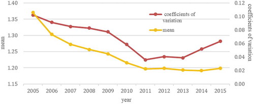
Looking at the coefficients of variation for green economic efficiency shown in Figure 2, it can be seen that these first fell and then rose, with the ultimate value smaller than the original value. This shows that regional differences in efficiency first narrowed and then expanded, but that the gap narrowed overall. Regional differences in the green economy were gradually reduced, but not to significant effect. Overall, between 2005 and 2015, green economic efficiency in the region presented a shift from “large gap and low level” to “relatively large gap and low level.”

Regional differences in green economic efficiency

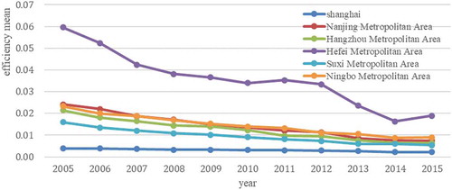
In order to explore the degree of deviation in green economic efficiency within the region, the average green economic efficiency values of the Yangtze River Delta urban agglomeration’s “one core and five areas” (one core: Shanghai; Nanjing metropolitan area: Nanjing, Zhenjiang, Yangzhou; Hangzhou metropolitan area: Hangzhou, Jiaxing, Huzhou, Shaoxing; Hefei metropolitan area: Hefei, Wuhu, Ma’anshan; Suzhou/Wuxi metropolitan area: Suzhou, Wuxi, Changzhou; Ningbo metropolitan area: Ningbo, Zhoushan, Taizhou) between 2005 and 2015 were individually calculated (Figure 3). The results showed: the difference in green economic efficiency between the Hefei metropolitan area and other areas is relatively large, but it is shrinking with each passing year. The Nanjing and Ningbo metropolitan areas have almost the same green economic efficiency values, while Shanghai showed low and relatively stable efficiency values despite being the most economically developed. Finally, the efficiency values of the Nanjing, Ningbo, Hangzhou, and Suzhou/Wuxi metropolitan areas are gradually becoming more uniform. The following is a ranking of areas from highest efficiency to lowest efficiency: Hefei metropolitan area > Nanjing, Ningbo metropolitan areas > Hangzhou metropolitan area > Suzhou/Wuxi metropolitan area > Shanghai.

Figure 3. Changes to the average green economic efficiency values of the Yangtze River Delta urban agglomeration’s “one core and five areas” between 2005 and 2015

Spatial evolution of green economic efficiency in the Yangtze River Delta urban agglomeration

Spatial structure of green economic efficiency

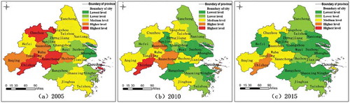
GIS natural breaks classification was used to divide the green economic efficiency levels of 26 cities in the Yangtze River Delta urban agglomeration into the high level, relatively high level, mid level, relatively low level, and low level categories, and the years 2005, 2010, and 2015 were selected as time points to carry out analysis of green economic efficiency’s spatial evolution (Figure 4). Overall, distribution is characterized by low green economic efficiency in the east and high efficiency in the west. More specifically, there are relatively few cities in the high level category, and these are mainly distributed in the northwest. In 2005, there were four high level cities in the southwest (Chizhou, Xuancheng, Chuzhou, Zhoushan), but by 2015 there were none. There are also very few cities in the relatively high level category, mainly distributed in the west and center. There were four of these cities in 2005 (Anqing, Wuhu, Ma’anshan, Huzhou), falling to one (Chizhou) by 2015. Cities in the mid level category showed a pattern of being distributed across multiple points but gradually becoming more concentrated toward the west. There were 11 cities in this category in 2005 (Hefei, Yancheng, Taizhou, Zhenjiang, Nantong, Yangzhou, Changzhou, Jiaxing, Shaoxing, Jinhua, Taizhou), falling to five cities in 2015 (Chuzhou, Wuhu, Ma’anshan, Xuancheng, Anqing). Relatively low level cities show a trend of spreading from Shanghai to the economically developed cities of each province. In 2005, there was just one (Shanghai), but by 2015 this had increased to ten (Hefei, Nanjing, Changzhou, Wuxi, Suzhou, Shanghai, Nantong, Hangzhou, Shaoxing, Ningbo). Low level cities are spread across the south and the coast. In 2005 there were five of these cities (Nanjing, Wuxi, Suzhou, Hangzhou, Ningbo), increasing to eight by 2015 (Yancheng, Yangzhou, Taizhou, Zhenjiang, Huzhou, Jiaxing, Jinhua, Taizhou).

Figure 4. Spatial distribution of green economic efficiency in the Yangtze River Delta urban agglomeration

Spatial cluster analysis of green economic efficiency

Urban agglomerations, as regions with a high degree of urban integration set against the backdrop of coordinated regional integration, have more refined transportation systems, closer economic links, and technological spillover that can spur the spatial dependence of various localities. Therefore, using the global Moran’s I index to carry out research of spatial correlations in green economic efficiency in the Yangtze River Delta urban agglomeration, it was possible to verify whether or not this correlation exists. The Moran’s I scatterplot (Figure 5) was obtained using Geoda’s queen contiguity weight matrix, and on this basis the spatial agglomeration characteristics of green economic efficiency in the years 2005, 2010, and 2015 were investigated.

Figure 5. Moran’s I index scatterplot of green economic efficiency in the Yangtze River Delta urban agglomeration

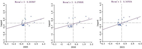
The results shown in Figure 5 indicate the following: (1) Global Moran’s I indexes for the years 2005, 2010, and 2015 were all greater than zero, which indicates that positive correlation exists in the green economic efficiency of cities in the Yangtze River Delta urban agglomeration. Furthermore, Z(I) values were all greater than 1.96, which indicates that results are significant at the level of 0.01, that statistical results are reliable, that there is obvious positive correlation overall, and that there is spatial agglomeration. (2) The Moran’s I index fell from 0.283567 in 2005 to 0.278595 in 2010, and then rose to 0.347634 in 2015, which shows that the progressing trend of spatial agglomeration weakened at first and then grew significantly stronger. (3) Distribution on the scatterplot shows an evolutionary trend from concentrated to scattered to reconcentrated, which indicates that development of the green economic efficiency of cities in the Yangtze River Delta urban agglomeration is imbalanced. (4) The number of points falling into the first quadrant gradually increased while the number of points falling into the third quadrant gradually decreased, indicating that the high to high agglomeration effect strengthened, while the low to low agglomeration effect gradually weakened.

Analysis of influencing factors in green economic efficiency

In order to explore the influencing mechanisms on green economic efficiency in the Yangtze River Delta urban agglomeration, seven factors were ultimately selected as variables of analysis by eliminating multicollinearity factors through variance factor inflation. These are: level of economic development, industrial structure, degree of economic openness, level of urbanization, government management, level of education, and level of scientific and technological innovation. Moreover, study of the Moran’s I index shows that clear spatial correlation exists in this region’s green economic efficiency. As a result, it was necessary to consider spatial effects, using a spatial econometric model to carry out regression analysis by making green economic efficiency the explained variable. In this model, PGDP represents GDP per capita to evaluate level of economic development; SPP represents secondary industry’s proportion of GDP and TPP represents tertiary industry’s proportion of GDP to evaluate industrial structure; FCP represents the proportion of GDP accounted for by actual utilization of foreign capital to evaluate degree of economic openness; UR represents the urban population’s share of the total population to evaluate level of urbanization; GEP represents the proportion of GDP accounted for by general government expenditures to evaluate government management; NUS represents the number of students enrolled at institutions of higher education to evaluate level of education; PAN represents the number of patent licenses to evaluate level of scientific and technological innovation; and GEE represents green economic efficiency. Since the attributes of time series data do not change after adopting the natural logarithm, and because this can make data incline to linearity and eliminate time series heteroscedasticity to a definite degree, the model employed index values derived from the natural logarithm.

For the convenience of comparison, a reliable curve function equation with a relatively optimal degree of fitting was reached. First, the least squares (OLS) method was used to carry out estimation of the general panel econometric model. Next, the maximum likelihood estimation method (ML) was used to carry out spatial panel econometric estimation of the model (11)~(13). Estimation and testing of the general panel model and the spatial panel econometric model was achieved through the respective support of Eviews 7.2 and Matlab 2017b software.

In estimating the general panel model, it was first necessary to choose a fixed effects model or a random effects model. Hausman testing showed that the statistic was 44.0300 with a corresponding P value of 0.0000, far lower than 0.05, rejecting the original assumption that individual effects are not related to regression variables (in which case a random effects model should be established), and therefore employing a fixed effects model was more reasonable. On this basis, estimation of three models was carried out: individual fixed effects, time fixed effects, and fixed effects. The results can be seen in Table 3. From adjusted R2 values, the fixed effects model’s values are larger compared to those of the other two models. Since the fixed effects model is better than the time fixed effects and individual fixed effects models, it should be applied in estimation of the general panel model.

Table 3. General panel estimation results

variable	Fixed period effect	Fixed Individual effect	Fixed effect
C	−6.2710***(0.0021)	−1.4151***(0.0015)	7.4526***(0.0077)
InPGDP	1.2633*(0.0539)	0.9699(0.4292)	2.007(0.0052)
InSPP	0.9633**(0.0321)	0.2550*(0.0777)	−0.2827*(0.0696)
InTPP	0.4849*(0.0696)	0.2121**(0.0215)	0.1571*(0.0632)
InFCP	−0.0031**(0.0478)	0.1190**(0.0450)	0.0890***(0.0010)
InUR	0.5495*(0.0512)	−0.5290**(0.0332)	0.1424*(0.0989)
InGEP	0.0029***(0.0012)	0.6269***(0.0089)	0.1314***(0.0077)
InPAN	0.3767***(0.0000)	0.0820***(0.0096)	0.0196***(0.0031)
InNUS	0.3712***(0.0000)	0.2254***(0.0091)	0.3820***(0.0015)
AdjR^2	0.8393	0.9029	0.9108
Log-likelihood	−146.3074	−69.2558	−51.7486
LM test no spatial lag			5.7475**(0.0170)
Robust LM test no spatial lag			1.7812**(0.0120)
LM test no spatial error			21.7365***(0.0000)
Robust LM test no spiatial error			17.7702***(0.0000)

*** indicates significant at the 1% level, ** indicates significant at the 5% level, and * indicates significant at the 10% level. Same as below.

Next, LM and Robust testing was applied to choose between the spatial error panel model (SEPDM) and the spatial lag panel model (SLPDM). The results (Table 3) show that SEPDM passed the 1% test while SLPDM passed the 5% significance test, with the former better than the latter. Comparison of the size of numerical values also backed up this conclusion, so the SEPDM was more suitable.

Then, the Wald test and the likelihood ratio (LR) test were used to judge whether the spatial Durban model (SDPDM) could be simplified as either the SLPDM or SEPDM. The Wald_spatial_lag and LR_spatial_lag values were 19.3204 and 19.3305 with probability of 0.0024 and 0.0037, respectively. Both passed significance tests at the 1% level, which indicates that in choosing an influencing mechanism model for green economic efficiency, the results of the SDPDM were better than those of the SEPDM, and therefore it was more suitable to apply the spatial Durban model.

After that, the Hausman test was used to determine whether a fixed effects model or a random effects model should be chosen for the spatial panel data econometric model. The results showed: the Hausman statistic was 0.4489, which means the significance level test was not passed. This indicated that the original assumption that individual effects are not related to explanatory variables could not be rejected, and the random effects spatial panel model should be adopted. Hausman test results for the standard panel and the spatial panel model were inconsistent. It is highly probable that a certain amount of deviation existed in the results of estimation using the least squares method since standard panel estimation did not incorporate spatial effects into the model. Therefore, it was more reasonable for this study to select the random effects spatial Durban model.

For the purposes of comparative analysis, this paper also carried out estimation of the SEPDM, the results of which can be seen in Table 4. From the results of estimating and testing the model, it is evident that: the random effects SDPDM log- likelihood value (−124.8394) was markedly better than that of the SEPDM (−141.9018). Meanwhile, the Corr-squared value was 0.9882, representing a relatively ideal fit. In sum, this study used the SDM with random effects to explore influencing mechanisms on green economic efficiency in the Yangtze River Delta urban agglomeration. From Table 4 it can be seen that the spillover effect coefficient (W*dep.var) has a positive value and passed the 1% significance level test, which indicates that spatial effects and positive spatial spillover effects exist in green economic efficiency in the Yangtze River Delta urban agglomeration. Therefore, in researching green economic efficiency in the Yangtze River Delta urban agglomeration, it is necessary to consider conditions of neighboring cities. At the same time, the above further illustrates the necessity of adopting a spatial econometric model to explore green economic efficiency’s influencing mechanisms.

Table 4. Random effects spatial Durbin model estimation results

Variable	Spatial error model	Spatial Dubin model	Variable	Spatial Dubin model
InPGDP	−0.0086(0.6969)	−0.0113(0.4823)	WInPGDP	0.0837(0.7021)
InSPP	0.2096(0.6514)	−0.0709(0.8768)	WInSPP	1.3240(0.1991)
InTPP	0.8109**(0.0257)	0.7861**(0.0282)	WInTPP	1.1753**(0.0676)
InFCP	0.0002***(0.0055)	0.1720***(0.0030)	WInFCP	−0.3175***(0.0000)
InUR	0.4735**(00219)	−0.5374**(0.0304)	WInUR	−0.5682(0.2736)
InGEP	0.1064***(0.0068)	0.0240***(0.0019)	WInGEP	0.0678(0.7008)
InPAN	0.3094***(0.0000)	0.2726***(0.0000)	WInPAN	0.0579**(0.0234)
InNUS	0.3793***(0.0000)	0.4153***(0.0000)	WInNUS	0.1672***(0.0189)
Log-likelihood	−141.9018	−124.8394	W*dep.var	0.2360***(0.0017)
Corr-squared	0.8462	0.9882

Looking at the elasticity coefficient of each variable, GDP per capita and secondary industry’s share of GDP did not pass significance tests, so these two variables had limited ability to analyze the model. Tertiary industry’s share of GDP had a positive coefficient and passed the 5% significance level test, which indicates that tertiary industry has a clear positive role in spurring green economic efficiency in the Yangtze River Delta urban agglomeration. That is, for every percentage point that tertiary industry’s share of GDP increases, efficiency increases by 0.79 of a percentage point. Degree of economic openness had a positive coefficient and passed the 1% significance level test, which shows that economic openness in the Yangtze River Delta urban agglomeration has a clear positive role in promoting green economic efficiency in this region. That is, for every percentage point that actual utilization of foreign capital increases, efficiency increases by 0.17 of a percentage point. Level of urbanization had a negative coefficient and passed the 5% significance level test, which indicates that urbanization has an inhibiting function on green economic efficiency in this region. Government management had a positive coefficient and passed the 1% significance test, which indicates that government expenditures have effectively advanced development of the region’s green economy. That is, for every percentage point that government expenditure’s share of GDP increases, efficiency increases by 0.02 of a percentage point. Level of scientific and technological innovation had a positive coefficient and passed the 1% significance level test, which shows that scientific and technological innovation and the development of education can effectively promote green economic efficiency in this region. By comparing elasticity coefficients, we can rank each influencing factor according to their degree of contribution to green economic efficiency: tertiary industry’s share of GDP > level of urbanization#> level of education > level of scientific and technological innovation > degree of economic openness > government management (# indicates a negative role). In terms of spatial lag parameters of explanatory variables, spatial spillover effects were ranked WInTPP>WInNUS>WInPAN>WInFCP#, with respective coefficients of 1.1753, 0.1672, 0.0579, and −0.3175. Each of these at least passed the 5% significance level test, which shows that tertiary industry, level of education, and level of scientific and technological development play a positive promoting role on green economic efficiency in surrounding areas, while degree of economic openness plays an inhibiting role. The lag parameters of other variables did not pass significance tests.

Conclusion and discussion

Main conclusions

This study followed the “process-pattern-mechanism” research approach. First, it innovatively adopted a composite “economy-society-resources-environment” perspective and applied a projection pursuit model and Super-DEA model considering undesirable outputs to establish a model for calculating green economic efficiency, which was used to measure green economic efficiency in the Pearl River Delta urban agglomeration. Next, it used spatiotemporal analysis to reveal the characteristics of green economic efficiency’s spatiotemporal evolution in this region. After that, it utilized a spatial econometric model to explore influencing mechanisms on green economic efficiency in the region. The following main conclusions were reached:

1. Green economic efficiency in the Pearl River Delta urban agglomeration is markedly lower than conventional green economic efficiency, with the gap between the two growing larger with each passing year. Conventional green economic efficiency has exaggerated the achievements of green development, and the state of public well-being in this region is in urgent need of improvement.

2. Green economic efficiency can be divided into clear stages overall. Efficiency values fell continuously between 2005 and 2010, while they tended to be stable and even showed signs of picking up slightly between 2010 and 2015. Regional differences gradually shrunk but not to noticeable effect, with an overall shift from “large gap, low level” to “relatively large gap, low level.”

3. The difference in green economic efficiency values between the Hefei metropolitan area and other areas is relatively large, but the gap is shrinking over time. The Nanjing and Ningbo metropolitan areas have almost identical green economic efficiency values, while Shanghai has a low and relatively stable value despite being the most economically developed. The efficiency values of the Nanjing, Ningbo, Hangzhou, Suzhou/Wuxi metropolitan areas are gradually becoming uniform. Overall, these areas can be ranked as follows: Hefei metropolitan area > Nanjing, Ningbo metropolitan areas > Hangzhou metropolitan area > Suzhou/Wuxi metropolitan area > Shanghai. On the whole, distribution of green economic efficiency is characterized by low values in the east and high values in the west with notable spatial agglomeration.

4. Results of empirical analysis showed that the spatial Durban model had superior fitting effects for exploring green economic efficiency in the Yangtze River Delta urban agglomeration. Within this model, tertiary industry’s share of GDP, degree of economic openness, government management, level of scientific and technological innovation, and level of education had positive influence on green economic efficiency in the region, while level of urbanization’s influence was negative. The influence of level of economic development and secondary industry’s share of GDP was not significant. At the same time, various factors had an influence on green economic efficiency that exceeded local areas. Tertiary industry, degree of economic openness, level of scientific and technological innovation, and level of education all had spatial spillover effects on surrounding areas.

5. The following is a ranking of influencing factors according to the intensity of their contribution to direct effects on local green economic efficiency: tertiary industry’s share of GDP > level of urbanization > level of education > level of scientific and technological innovation > degree of economic openness > government management. Ranked according to spatial spillover effects on surrounding areas: tertiary industry’s share of GDP > level of education > level of scientific and technological innovation > degree of economic openness.

Discussion

1. Green economic efficiency is reflected in the economy, resources, and the environment, but even more so in human welfare and the well-being of society. The green economy is a developmental model that integrates the economy, society, resources, and the environment. The meaning of green economic efficiency is not only limited to resource and environmental constraints. Instead, it should be emphasized that the ultimate goal of green development is to improve public well-being. Socialism with Chinese Characteristics for a New Era has also introduced higher requirements in this respect, and green economic efficiency under the “economy-society-resources-environment” perspective has provided our research with a new angle. Therefore, green economic efficiency under this composite perspective fully embodies the meaning of the green economy and can reflect what is necessary under current national conditions. It is precisely on this basis that this paper established a model for calculating green economic efficiency under a new perspective, finding that conventional green economic efficiency has exaggerated the reality in its evaluation of the real state and results of green economic development, which is clearly detrimental for a China that is in the process of transforming its development. However, due to factors such as the availability and real workability of data, the composite perspective green economic efficiency calculation model established in this paper still needs to be improved in some areas. For example, it was not possible to prove the applicability of the combination used in the model (projection pursuit and Super-DEA model considering undesirable output), so further exploration and practice is required in this regard, and index selection in efficiency calculation was overly weighted to education, so subsequent studies need to improve upon this.

2. This paper showed that GDP and secondary industry’s share of GDP do not have significant direct influence on green economic efficiency, a conclusion which differs from those of some scholars. Previous research has shown that a “U”-shaped relationship exists between GDP and green economic efficiency, with the belief that China’s economic development initially followed an extensive growth model in which resources and the environment were sacrificed and size was pursued while quality was ignored, leading to a drop in green economic efficiency. Later on, as China began to pay greater attention to resource and environmental issues, the country gradually shifted toward a model of development featuring conservation of resources and environmental friendliness, which has been accompanied by a gradual rise in green economic efficiency even though the GDP growth rate has somewhat slowed. Secondary industry is largely composed of industries that are not green, and therefore growth of its share inevitably brings additional resource and environment related costs, which causes a drop in green economic efficiency. It is highly possible that updating of green economic efficiency’s meaning caused this study to indicate that these two factors showed insignificant influence. Further verification should be carried out in the future to determine whether discrepancy actually exists between green economic efficiency under the new perspective and green economic efficiency under resource and environmental constraints (conventional), or whether this is a result of regional factors.

3. Increasing green economic efficiency in the Yangtze River Delta urban agglomeration can start from enhancing tertiary industry’s share of GDP, degree of economic openness, government administration, level of scientific and technological innovation, or level of education, or promoting the progress of quality-oriented urbanization. At the same time, the spatial spillover effects of each factor should be considered, and emphasis should be placed on coordination and joint action between regions. Other than level of urbanization (which is also different from the existing research), other factors all have a positive influence on green economic efficiency in the region. The negative influence of level of urbanization stems from the fact that rapid urbanization has pulled the urban-rural gap wider and lowered social equity, thereby inhibiting the rise of green economic efficiency. From now on, emphasis should be placed on coordinated development between urban and rural areas, rural vitalization and urban development should advance in a concerted manner, and quality-oriented urbanization should be promoted. The spatial spillover effects of green economic efficiency, tertiary industry, degree of economic openness, level of scientific and technological development, and level of education show that developmental connections exist between regions. With their high levels of urban integration, urban agglomerations are the main players in China’s new urbanization, and developing urban agglomerations should mean putting focus on coordinated regional development. The green development of urban agglomerations should not only take advantage of existing factors with regional spillover effects, but also tap into factors with potential spillover effects (like government management) in order to better serve the shift toward green development.

Disclosure statement

No potential conflict of interest was reported by the authors.

Additional information

Funding

This work was supported by the National Key Research and Development Plan of China [2017YFC0505702].

References

- Barbier, E. B. 2010. A Global Green New Deal: Rethinking the Economic Recovery[M]. London: Cambridge University press.
- Coelli, T., L. Lauwers, and V. H. Guido. 2005. “Formulation of Technical, Economic and Environmental Efficiency Measures that are Consistent with the Materials Balance Condition [EB/OL].” .CEPA Working Paper Series, No .06/2005.
- Cui, Q., and Y. Li. 2015. “An Empirical Study on the Influencing Factors of Transportation Carbon Efficiency: Evidences from fifteen Countries.” Applied Energy 141: 209–217. doi:10.1016/j.apenergy.2014.12.040.
- Domazlicky, B. R., and W. L. Weber. 2004. “Does Environmental Protection Lead to Slower Productivity Growth in the Chemical Industry?[J].” Environmental and Resource Economics 28 (3): 301–324. doi:10.1023/B:EARE.0000031056.93333.3a.
- Elhorst, J. P. 2014. Econometrics: From Cross-Sectional Data to Spatial Panels [M]. New York: Springer.
- Flavius, B. 2015. “Ranking Trade Resistance Variables Using Data Envelopment analysis[J].” European Journal of Operational Research 247 (3): 978–986. doi:10.1016/j.ejor.2015.05.062.
- Fukuyama, H., and W. L. Weber. 2010. “A Slacks-Based Inefficiency Measure for A Two Stage System with Bad outputs[J].” Omega 38 (5): 398–409a. doi:10.1016/j.omega.2009.10.006.
- Hailu, A., and T. S. Veeman. 2001. “Non-Parametric Productivity Analysis with Undesirable Outputs: An Application to the Canadian Pul Pand Paper Industry[J].” American Journal of Agricultural Economics 83: 605–616. doi:10.1111/0002-9092.00181.
- Korhonen, P. J., and M. Luptacik. 2004. “Eco-Efficiency Analysis of Power Plants: An Extension of Data Envelopment Analysis[J].” European Journal of Operational Research 154 (2): 437–446. doi:10.1016/S0377-2217(03)00180-2.
- Kuang, Y., and D. Peng. 2012. “Analysis of Environmental Production Efficiency and Environmental Total Factor Productivity in China.” Economic Research Journal 47 (7): 62–74.
- Kumar, P. 2017. “Innovative Tools and New Metrics for Inclusive Green economy[J].” Current Opinion in Environmental Sustainability 24: 47–51. doi:10.1016/j.cosust.2017.01.012.
- Kumar, S. 2006. “Environmentally Sensitive Productivity Growth: A Global Analysis Using Malmquist–Luenberger index[J].” Ecological Economics 56 (2): 280–293. doi:10.1016/j.ecolecon.2005.02.004.
- Lan, Z., and M. Huang. 2018. “Safety Assessment for Seawall Based on Constrained Maximum Entropy Projection Pursuit model[J].” Natural Hazards 91 (3): 1165–1178. doi:10.1007/s11069-018-3172-8.
- Li, H., and J. F. Shi. 2014. “Energy Efficiency Analysis in Chinese Industrial Sectors: An Improved Super-SBM Model with Undesirable outputs[J].” Journal of Cleaner Production 65 (4): 97–107. doi:10.1016/j.jclepro.2013.09.035.
- Li, Y., and M. Hua. 2014. “Green Efficiency of Chinese Cities: Measurement and Influencing Factors.” Urban and Environmental Studies 2 (1): 36–52.
- Lin, B., and H. Long. 2015. “A Stochastic Frontier Analysis of Energy Efficiency of China’s Chemical industry[J].” Journal of Cleaner Production 87 (1): 235–244. doi:10.1016/j.jclepro.2014.08.104.
- Liu, H., C. Fang, X. Zhang, Z. Wang, C. Bao, and F. Li. 2017. “The Effect of Natural and Anthropogenic Factors on Haze Pollution in Chinese Cities: A Spatial Econometrics approach[J].” Journal of Cleaner Production 07: 127.
- Loiseau E, Saikku L, Antikainen R 2016. “Green Economy and Related Concepts: An overview[J]”. Journal of Cleaner Production 139: 361–371. doi: 10.1016/j.jclepro.2016.08.024.
- Long, Y., and H. Xiaozhen. 2012. “Analysis on Regional Difference and Convergence of theEfficiency of China’s Green Economy Based on DEA[J].” Economist (2): 46–54.
- Mahdiloo, M., M. Toloo, T. T. Duong, R. F. Saen, and P. Tatham. 2018. “Integrated Data Envelopment Analysis: Linear Vs Nonlinear Model.” European Journal of Operational Research 268 (1): 255–267.
- Mei G, Dong L, Tian C. 2014. “The Research for Liaoning Environmental Efficiency and Spatial-Temporal differentiation[J].” Geographical Research 16 (3): 170–178.
- Nikolaus, E. 2015. “Evaluating Capital and Operating Cost Efficiency of Offshore Wind Farms: A DEA approach[J].” Renewable and Sustainable Energy Reviews 42: 1034–1046. doi:10.1016/j.rser.2014.10.071.
- Qian, Z. M., and X. C. Liu. 2013. “Regional Differences in China’s Green Economic Efficiency and Their Determinants.” China Population Resources and Environment 23(7): 104–109.
- Ramanathan, R. 2005. “An Analysis of Energy Consumption and Carbon Dioxide Emissions in Countries of the Middle East and North Africa[J].” Energy 30 (15): 2831–2842.
- Scheel, H. 2001. “Undesirable Outputs in Efficiency valuations[J].” European Journal of Operational Research 132 (2): 400–410. doi:10.1016/S0377-2217(00)00160-0.
- Seiford, L. M., and J. Zhu. 2002. “Modeling Undesirable Factors in efficiency evaluation[J].” European Journal of Operational Research, no. 142: 16–20. doi:10.1016/S0377-2217(01)00293-4.
- Song M L, Zhang LL, Liu W. 2013. “Bootstrap-DEA Analysis of BRICS’ energy Efficiency Based on Small Sample data[J]”. Applied Energy 112: 1049–1055. doi: 10.1016/j.apenergy.2013.02.064.
- Tao, X., P. Wang, and B. Zhu. 2016. “Provincial Green Economic Efficiency of China: A Non-Separable Input–Output SBM approach[J].” Applied Energy 171: 58–66. doi:10.1016/j.apenergy.2016.02.133.
- Tone, K. 2003. “Dealing with Undesirable Outputs in DEA: a Slacksbased Measure (SBM) Approach[R].” GRIPS Research Report Series 118–120.
- Toshiyuki, S., and G. Mika. 2014. “DEA Radial Measurement for Environmental Assessment: A Comparative Study between Japanese Chemical and Pharmaceutical firms[J].” Applied Energy 115: 502–513. doi:10.1016/j.apenergy.2013.10.014.
- UNEP. 2011. “Green Economy: Pathways to Sustainable Development and Poverty Eradication[J].” Nairobi Kenya Unep 12–15.
- Wang,L., Y. Lian, and X. Chen. 2018. “Quantifying the Contribution of Flood Intensity Indicators with the Projection Pursuit Model.” Hydrology Research 49 (1): 60–71.
- Yörük, B. K., and O. Zaim. 2005. “Productivity Growth in OECD Countries: A Comparison with Malmquist indices[J].” Journal of Comparative Economics 33 (2): 401–420. doi:10.1016/j.jce.2005.03.011.
- Young, A. 2000. “Gold into Base Metals: Productivity Growth in the People’s Republic of China during the Reform Period[J].” Nber Working Papers 111 (6): 1220–1261.
- Yu, S., and H. Lu. 2018. “An Integrated Model of Water Resources Optimization Allocation Based on Projection Pursuit Model - Grey Wolf Optimization Method in a Transboundary River basin[J].” Journal of Hydrology. doi:10.1016/j.jhydrol.2018.02.033.
- Zhu, D. J. 2012. “New Concept and Trend of Green Economy Emerging from Rio+20[J].” China Population Resources and Environment.