Comprehensive assessment on the ecological stress of rapid land urbanization per proportion, intensity, and location

ABSTRACT

Aiming at assessing the ecological stress of land urbanization comprehensively, three perspectives are considered and combined, i.e. the amount effect with the proportion of construction lands as the indicator, the intensity effect per the density of environmental pollutant emissions, and the location effect based on their spatial distribution in the heterogeneous landscape. The quantitative results of Southern Jiangsu case in Eastern China show the single-perspective ecological stress are spatially different; the proportion effect is higher in city propers which are more densely populated and industrialized. However, the intensity effect is more significant for units along the Yangtze river where heavy industries are gathered, while the location effect is higher in “ecologically suitable” regions. As the integration of proportion, intensity, and location effects, the comprehensive stress differs across Southern Jiangsu and are also different with the single-perspective results. Dominant stressors of each unit are spatially distinct, which benefits policy-makers in targeting their objectives as per primary influencing factors. It is concluded that the comprehensive assessment could efficiently reveal the spatial differentiation of the ecological effects of land urbanization and also the differentiated role of different factors for each unit.

KEYWORDS:

• Comprehensive ecological stress
• land urbanization
• land use intensity
• location effect
• Eastern China

Introduction

Urbanization remits economic development and improved standards of living, but also causes unprecedented and often dramatic changes in land use and land cover (Turner et al. 1990). The spatial expansion of construction lands due to urbanization has various ecological effects which well merit governmental concern as well as scholarly attention (Buttel 2000; Li, Chen, and Fan 2011). Comprehensive data reflecting the ecological effects of land urbanization underlie many ecological protection and restoration policies (Lambin et al. 2001; Peng et al. 2017). The negative effects of land urbanization, or so-called “ecological stress,” may constitute an urgent issue in regards to policy orientations on land-use regulation and adjustment (He et al. 2011; Seto, Güneralp, and Hutyrac 2012).

Many researches have been published on assessing the ecological stress of land urbanization from various perspectives. The most widely adopted methodology focuses on the structure and function changes of ecosystem with various indicators or metrics (He et al. 2011; Dupras et al. 2016). Among which, some evaluate the function changes of the ecosystem through certain comprehensive indicators including ecosystem services (Daily 1997; Sieber and Pons 2015), ecological vulnerability (Li and Fan 2014; Nguyen et al. 2016), ecological resilience (Saunders and Becker 2015), etc. Besides, some specific indicators are emphasized to represent certain effect accurately. Under the context of environmental change, the effect on regional/local climate is receiving more emphasis (Zhao et al. 2015), and the perspective of urban temperature and rain effect is among the most concerned aspects (Grimm et al. 2008; Chen et al. 2019; Su et al. 2019). The conservation biologists also analyze the changes of biodiversity during land urbanization and indicate the expansion of construction lands and induced habitat fragmentation are among the main stressors for biodiversity loss (Horvath et al. 2019). There are still researches focusing on water or soil environment changes related with land urbanization (Imhoff et al. 1997; Shi et al. 2019). Recently, some researchers emphasize the structure changes of the ecosystem with different landscape-level metrics, such as number of patches, edge density, landscape shape index, contagion index, diversity index, ecological connectivity, etc. (e.g., Tian, Chen, and Yu 2014; Sakieh et al. 2015; Estoque and Murayama 2016). Though the above techniques effectively reflect the quality or changes in a given regional ecosystem, they solely involve regional ecosystem. As land development significantly affects the regional ecosystem, land use should be emphasized in ecological effect evaluation (Li, Gao, and Chen 2019).

Considering the various attributes of construction lands, different perspectives have been adopted to assess their ecological effect with relevant indicators (Peng et al. 2017). Up to now, the most direct indicator centers on the area (or proportion) of construction lands (or “built-up areas”) within a certain region, which is a considerable simplification of the whole area and construction lands (Li, Gao, and Chen 2019). As per its simplicity and accessibility, the amount/proportion indicator is commonly used to indicate the extent of land development for the purposes of cross-regional comparison or as a sub-indicator for land development assessment (van Diggelen et al. 2005; Fan et al. 2012). It is also often used as a pre-controlling parameter for governmental regulation on regional land development, such as for land-use plans in China, where suitable lands for urbanization and industrialization are quantitatively limited (Liu, Fang, and Li 2014).

The proportion of construction lands is directly related to the ecological stress of land urbanization, but they do not simply form a proportion as they are not homogeneous or undifferentiated, which is reflected by various attributes including land-use intensity (LUI) (Lambin, Rounsevell, and Geist 2000; Brown and Reiss 2010; Erb, Haberl, and Rudbeck 2013). The LUI concept was initially proposed to indicate the output of agricultural-use lands as-expressed by the quantity of agricultural products from arable areas (Turner and Doolittle 1978; Jiang, Deng, and Seto 2013). As a comprehensive indicator containing a variety of intensive land-use indicators, LUI has been widely adopted in land urbanization research to reflect the status or function of construction lands according to population agglomeration, economic development, investments, resource consumption, pollutant emissions, and other indicators (Ellis and Ramankutty 2008; Gong et al. 2014). Basically, higher LUI means more population or industry are concentrated within limited lands (Xie et al. 2018; Zhu et al. 2019).

Intensive land use implies that less lands are occupied for regional development, so more lands could be reserved for agricultural production and ecological protection. Although it brings socio-economic benefits and is specially encouraged in areas with limited suitable lands, it also consumes resources and causes a sizable increase in pollutant emissions which places the region under increasing ecological stress (Zampella et al. 2007; Long et al. 2014). Although many researchers have indicated that extensive expansion of construction lands and induced industrial development are the main causes underlying the rapid increase in energy consumption and pollutant emissions (e.g., Huang et al. 2016; Feng et al. 2018), there are some reports indicating carbon emissions per amount of GDP would decline with intensive land use (Xu, Guo, and Chen 2013; Xie et al. 2018). However, few researchers have analyzed the density of pollutant emissions per area of construction lands and indicated the intensity effect from the perspective of pollutant emissions, as the emissions rather directly connect environmental pollutants to industrial development and population agglomeration (Grossman and Krueger 1995; Cherniwchan 2012). The density of undesired environmental outputs is related to various attributes of land use including the main functions, industries, or population/economy agglomeration degree of construction lands (Zhang, Zhang, and Dong 2013). Comparing with the amount of construction lands, the density of undesired environmental outputs is also of significance for assessing the integrated ecological effect of land urbanization. To this effect, LUI must be taken into account when assessing the ecological stress of land urbanization.

Other perspectives in addition to proportion and intensity affect the differentiation of ecological stress from land urbanization, including the location or spatial position effects under spatially differentiated ecosystems (Dadashpoor, Azizi, and Moghadasi 2019). The ecological effects of construction lands are spatially different or location-related (He et al. 2011; Li, Gao, and Chen 2019). Various landscape-level metrics have been proposed to reflect the changes in landscape patterns caused by land-use changes, which mostly center on the general landscape structure including all land-use types (e.g., Sakieh et al. 2015; Dupras et al. 2016; Carlier and Moran 2019). However, little attention has been paid to specific spaces occupied by land urbanization in a heterogeneous landscape. The spatial heterogeneity of ecosystems should be taken into account as the location effect is spatially explicit (He et al. 2011). Up to now, most researchers have observed spatial heterogeneity from the perspective of stable features including biodiversity (Jackson, Walker, and Gaston 2009; Blasi et al. 2011; Marignani and Blasi 2012), ecosystem service functions (Wang et al. 2019), and ecological carrying capacity (Irankhahi et al. 2017) while generally neglecting the significance of ecological process (EP) dynamics (Xiang and Meng 2016; Li, Gao, and Chen 2019). Considering the importance of EP in ecological conservation, construction lands should be placed into the EP to determine their location effects in terms of ecological stress.

The proportion, intensity, and location of construction lands are not the only meaningful factors but are among the most significant causes of differentiated ecological stress. Single-perspective assessment is insufficient. Targeted policy-making must be informed by detailed information to effectively optimize land development according to the primary factor inducing ecological stress. Land-use policy in China and certain other countries centers on the amount, intensity, and location of construction lands. In the Outline of National Land Use General Plan in China (2006–2020) published by the State Council of China, related statements include i) controlling the amount of construction lands, ii) promoting the coordination of population & economy agglomeration and the resources development & environment protection; and iii) optimizing the spatial distribution of existing and incremental construction lands. The governmental focus further indicates the major concerns in land-use regulation.

Therefore, based on theoretical implications and practical requirements, we conducted a comprehensive assessment of the ecological stress of land urbanization in a rapidly urbanized region in Eastern China, i.e., Southern Jiangsu. We addressed the following questions: 1) How does one evaluate the comprehensive ecological stress of land urbanization from various perspectives including proportion, intensity, and location – particularly the location effect related to the spatial heterogeneity of ecosystems? 2) What is the spatial pattern of comprehensive ecological stress? Are there any differences among spatial patterns based on the proportion, intensity, and location effects of construction lands? 3) Which factors dominate the comprehensive ecological stress of different units? Are there any policy implications for further land-use regulations?

Study area and methodology

Study area

Southern Jiangsu is located in the Yangtze River Delta Urban Agglomeration (YRDUA) and is one of the most ecologically livable regions in Eastern China as well as one of the most developed and modernized regions throughout the country (Zhong, Chen, and Huang 2016). It contains five prefectural cites (Nanjing, Wuxi, Changzhou, Suzhou, and Zhenjiang) and can be further divided into 33 county-level units (Figure 1; Table 1). In 2015, the construction lands in Southern Jiangsu had reached about 6,617 km², or 23.45% of the total area and 5.7 times the national average. The expansion of construction lands was spatially different; thus, the caused ecological stress of land urbanization may be quite different. Meanwhile, the land urbanization and related population agglomeration and industrial development caused large amounts of pollutant emissions including SO₂ and NO_x, which were 413 and 438 thousand tons in 2015, respectively. The emissions were also spatially different as unlike amount and function of construction lands in different units. Besides, the spatial distribution of construction lands might also cause the differentiation of ecological stress as some occupied more important ecological lands. To enhance scientific cognition and afford targeted measures for regulating regional land-use patterns, as discussed above, we chose to comprehensively assess the ecological stress of land urbanization per proportion, intensity, and location of construction lands.

Figure 1. Location, administrative divisions and land-use in Southern Jiangsu in 2015

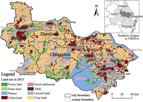
Table 1. Administrative divisions and grassroot organizations in Southern Jiangsu, 2015

prefectural city	Land area (sq. km)	Construction land (sq. km)	SO2 emission (thousand tons)	NOx emission (thousand tons)	District	County
Nanjing	6587.02	1540.68	102.77	96.12	City proper of Nanjing, Jiangning, Luhe, Pukou, Lishui, Gaochun	/
Wuxi	4627.91	1215.64	76.62	98.14	City proper of Wuxi, Xishan, Huishan, Xinwu, Binhu	Jiangyin, Yixing
Changzhou	4372.14	923.92	34.51	59.09	City proper of Changzhou, Xinbei, Wujin, Jintan	Liyang
Suzhou	8657.31	2204.70	150.79	140.26	City proper of Suzhou, Xiangcheng, Wuhzhong, Wujiang, Suzhou New District, Suzhou Industrial Park	Changshu, Kunshan, Zhangjiagang, Taicang
Zhenjiang	3840.32	732.53	48.70	44.82	City proper of Zhenjiang, Dantu	Danyang, Jurong, Yangzhong

Data source: Jiangsu Statistical Yearbook (2016) and environmental statistics in 2016.

Methodology

Calculation of proportion effect: P stress value

The proportion effect of the ecological stress of land urbanization is related to the amount of construction lands and the area of the evaluation unit, i.e., the “quantity-oriented ecological stress of construction lands” (Li, Gao, and Chen 2019). This indicator is popular among researchers for its simplicity and feasibility in cross-region comparison. It is expressed as follows:

(1) $p_k=\frac{\frac{A_k}{T_k}\times 100}{\frac{{\sum }_{k=1}^n{A}_k}{{\sum }_{k=1}^n{T}_k}\times 100}$(1)

where p_k is the proportion effect of construction lands of unit k; A_k is the area of construction lands in unit k; T_k is the total area of unit k; k is the number of units, i.e., 33. We standardized the proportion of each unit by comparing it against the regional average to complete a cross-region comparison and eliminate the effect of absolute value.

Calculation of intensity effect: I stress value

As mentioned above, the ecological stress of construction lands is affected by resource consumption and undesired outputs including environmental pollutants (Zhao et al. 2006). Some construction lands produce more environmental pollutants than the others, thus they are regarded to be more “stressful.” Considering the data representativeness and availability, we chose SO₂ and NO_x as the inputs for evaluating LUI and calculated this indicator as follows:

(2) ${\mathrm{i}}_k=\frac{\frac{\mathrm{S}{\mathrm{O}}_{2-k}}{A_k}}{\frac{{\sum }_{k=1}^{n}S{O}_{2-k}}{{\sum }_{k=1}^n{A}_k}}\times 0.5+\frac{\frac{N{O}_{x-k}}{A_k}}{\frac{{\sum }_{k=1}^{n}N{O}_{x-k}}{{\sum }_{k=1}^n{A}_k}}\times 0.5$(2)

where i_k is the intensity stress value of construction lands in unit k;SO_2−k and NO_x-k are the emission amount of SO₂ and NO_x of unit k; k has the same meaning in Formula (1). There are three main types of environmental pollutants: water, air, and soil. The most widely adopted indicators of water pollutants include COD and BOD, which are also the results of agricultural production and were neglected here to zero in on the effects of construction-related pollutants; soil pollutants was also neglected as they are difficult to quantify. We adopted major air pollutants SO₂ and NO_x as the pollutant indicator as they are significant overall and can be easily quantified based on county-level governmental statistics of Jiangsu and the five prefectural cites. Almost all SO₂ and NO_x are emitted in secondary and tertiary industries concentrated in construction lands. The emissions of SO₂ and NO_x are of significant consistency and difficult to assess their weight separately, so we used the average intensity of SO₂ and NO_x to represent the comprehensive value after standardization by the regional average value.

Calculation of location effect: L stress value

Construction lands in regions with higher ecological suitability tend to have higher ecological stress than construction lands in less ecologically suitable areas (Li, Gao, and Chen 2019). Considering the significance of potential EP in maintaining necessary functions, we carried out EP analysis to indicate the spatial heterogeneity of ecological suitability, then divided Southern Jiangsu into ecological zones with varying suitability. By identifying construction lands in different ecological zones and with the corresponding level of stress, we calculated the location effect via weighted summing of these factors.

1. Model introduction for EP simulation

EP analysis reveals the spatial heterogeneity of ecological suitability for relevant ecological zoning, and simulations with suitable ecological models are often adopted to indicate potential EP where field investigation is highly time-consuming in a vast region with complicated ecosystem structures. The MCR model has theoretical reasonableness and technological availability with a widely recognized tool box and algorithm support in GIS packages (Gonzalez, Del Barrio, and Duguy 2008). It is also recognized as a means for cost-distance analysis, and was first used to simulate landscape connectivity and key step-stones based on the dispersal of certain species (e.g., Ferreras 2001; Schadt et al. 2002). The expansion of ecological spaces is an abstraction of species dispersal, so the originally species-specific method can also be used to modify the potential expansion of ecological spaces (Adriaensen et al. 2003; Liu, Shu, and Zhang 2010). Further, MCR model has been used in ecological zoning as the cumulative values in the simulation results reflect the suitability in maintaining necessary EP (Ye et al. 2015; Xiang and Meng 2016). According to methods described by Knappen, Scheffer, and Harms (1992), Yu (1996) and Li et al. (2015), EP can indeed be simulated by MCR analysis when expressed as follows:

(3) $MCR=f_{min}\sum _{j=n}^{i=m}{D}_{ij}\times R_i$(3)

where f is a function of the positive correlation, which reflects the relation of the least resistance for any point in space to the distance from any point to any source and the characteristics of the landscape base surface; min denotes the minimum value of cumulative resistance produced in different processes of landscape unit i transforming into a different source unit j; D_ij is the spatial distance between landscape unit i and source unit j; R_i denotes the resistance coefficient that exists in dispersal from landscape unit i to source unit j (Li et al. 2015).

• (2)Model variables

ArcGIS spatial analysis software and its cost-distance module are the most commonly used tools for MCR analysis. The necessary variables include source, target and resistance surface.

Source: Source, which is also the target in the landscape ecology, refers to a landscape type that supplies valuable ecosystem services and promotes EP development (Adriaensen et al. 2003; Li et al. 2015). It is identified based on important ecological function protection areas in the Jiangsu Major Function Oriented Zoning (JMFOZ), where important ecological function protection areas are defined as spaces with significant natural/cultural value including nature reserves, forest parks, scenic areas, geo-parks, drinking water protection areas, flood storage and detention basins, fishery and aquatic resource protection areas, important wetlands, water-dilution channels, ecological forests, and water conservation and reserve areas (Figure 2(a)). Large water bodies such as Taihu Lake, Gehu Lake, and Yangtze River are also taken into account for their ecological significance. The total area of these sources is about 7,055 km² accounting for 25% of the study area.

Figure 2. Ecological lands and resistance surface in Southern Jiangsu

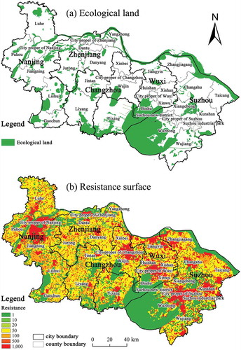
Resistance surface: It is designed based on the resistance values of different land-use classes which are relative and have different extensions (Villalba et al. 1998; Schadt et al. 2002). To model the dispersal of certain species, researchers typically determine the explicit value of certain land-use classes by expert assignment or field investigation (Ferreras 2001; Schadt et al. 2002; Li et al. 2015). The target of our research is ecological space rather than certain species, so the resistance value of a certain land-use class represents the level of difficulty of that patch becoming ecological land. Therefore, it is impossible to design species-specific resistance values or corresponding resistance surfaces.

Some researchers consider land-use classes with higher ecosystem productivity/services or lower levels of anthropogenic disturbance to be more suitable and have lower resistance to the expansion of ecological lands (Li et al. 2015). Nature reserves, forests, and water bodies are regarded as the most-suitable ecological lands and assigned lower resistance values. Construction lands or built-up areas have high levels of anthropogenic disturbance and are least-suitable for the expansion of ecological lands, thus they are assigned the highest resistance values. Cultivated lands and grasslands have medium-level resistance values. It is necessary to determine the extension of resistance values or assign explicit values to certain land-use classes as well, and existing researches have made quite different assignment, such as 1–5 (Liu, Shu, and Zhang 2010; Li et al. 2015), 0–500 (Su et al. 2016), and 1–500 (Li, Chen, and Fan 2011). Basically, larger relative differences between land cover classes deviate further from the default straight line between source and target patches (Adriaensen et al. 2003).

The adopted land-use data encompass six land-use types (crop land, forest land, grass land, waters, construction land, and unused land) with 25 sub-types (Ning et al. 2018). Only 15 of the sub-types are found in Southern Jiangsu (Table 2). Woodlands and water bodies are the most suitable ecological lands, so they were assigned with resistance of 1. In determining the extension and resistance value of other land-use classes, we enlarged the resistance values of least-suitable land (urban land) to make them reflect the intensity of anthropogenic disturbance. After testing several values, we found that 1,000 is sufficient as per the expansion of ecological space. The population density of urban lands exceeds 10,000 people per km² averagely, which is about 1,000 times that of the most sparse areas. Therefore, we assigned them resistance of 1,000 to reflect the extent of anthropogenic disturbance. The resistance values of other land-use types were determined based on the extent of resistance from 1 to 1000 and experts judgment (Table 2). A resistance surface map of Southern Jiangsu was obtained with grid size of 1 km × 1 km based on the land-use map (Figure 2(b)).

Table 2. Resistance value of different types of land use

Type	Type name	Sub-type	Sub-type name	Resistance value
1	Crop land	11	Paddy land	100
		12	Dry land	200
2	Forest land	21	Woodland	1
		22	Shrubbery land	5
		23	Sparsely forested land	10
		24	Other forest land	10
3	Grass land	31	High coverage grassland	10
4	Waters	41	River	1
		42	Lake	1
		43	Reservoir and pond	1
		46	Floodplain	1
5	Construction land	51	Urban land	1000
		52	Rural resident	500
		53	Independent industrial and mining land (IIML)	500
6	Unused land	66	Exposed rocky and gravel land	100

In the result of MCR analysis, no maximum value was set to ensure that all grids could be fully quantitatively compared for zoning of the whole region.

• (3) Ecological zoning based on EP simulation

Based on the MCR analysis, grids with lower MCR value have higher accessibility and are more suitable for the expansion of ecological space, so they are well suited to maintaining EP (Adriaensen et al. 2003; Li et al. 2015). Accordingly, the ecological zone with higher MCR is of lower ecological suitability, and construction lands in less suitable ecological zones are with lower ecological stress. To quantitatively evaluate the location effects of construction lands, it is necessary to define the stress value of construction lands in different ecological zones. As no widely accepted quantitative criteria for determining the levels of ecological zones, we chose to divide the whole region into a 10-level ecological zone with varying ecological suitability based on MCR values using the Classification by “Natural Breaks (Jenks)” tool in ArcGIS software which can minimize the differences within groups and maximize the differences between groups. We assigned the construction lands in the 10 levels of ecological zones values from 10–1 as per the highest to lowest ecological suitability, or lowest to highest MCR values. As the following calculation of regional-level stress values of the evaluating units would be standardized by comparing them against the regional average value, the results were not significantly affected by the number of levels or precise stress values of each level of ecological stress.

• (4) Quantitative calculation of location effect

The location effect is related to both the spatial distribution of construction lands and the spatial heterogeneity of ecological suitability. After an overlaying analysis of construction lands and ecological zones, the amount of construction lands of each unit in the 10 ecological zones was determined and used to calculate the location effect and comprehensive stress value in combination with the other effects discussed above.

(4) $l_{\mathrm{k}}=\frac{\frac{{\sum }_{j=1}^m{A}_{kj}\times s_j}{A_k}}{\frac{{\sum }_{k=1}^n{\sum }_{j=1}^m{A}_{kj}\times s_j}{{\sum }_{k=1}^n{A}_k}}$(4)

where l_k is the location stress value of construction lands in unit k; A_kj is the area of construction lands in unit k and ecological zone j, S_j is the ecological stress index of construction lands in ecological zone j; j is the total number of ecological zones (10 in our case); k has same meaning as in Formula (1). As mentioned above, S_j is 10 for construction lands distributed at ecological zones with the lowest MCR value and corresponding highest ecological suitability; it is 1 for the least-suitable ecological zone. Similar to p_k and i_k, we standardized the location effect of each unit by comparison against the regional average value.

Calculation of comprehensive ecological stress

It is necessary to combine the three indicators of proportion, intensity, and location effects to obtain the comprehensive stress value. Among lots of methods available for integrating the stress values, we chose to multiply the three values considering their undifferentiated effects on ecological stress and to emphasize the regional differences.

(5) $PI{L}_k=p_k\times i_k\times l_k$(5)

where PIL_k is the comprehensive stress value after integrating proportion, intensity, and location effects of unit k; p_k, i_k and l_k are the respective proportion, intensity, and location stress values.

Identification of dominant stressors

Dominant stressors, or influencing factors, were analyzed based on the differentiated stress values of proportion, intensity, and location across the 33 units. With standardized p_k,’ i_k,’ and l_k’ ranging from 0 to 1, the highest one indicates the dominant stressor. The standardization for p_k,’ as an example, was conducted as follows:

(6) ${p_{\mathrm{k}}}^{\prime }=\frac{p_k-min(p_1,p_2,\cdot \cdot \cdot ,p_{33})}{max(p_1,p_2,\cdot \cdot \cdot ,p_{33})-min(p_1,p_2,\cdot \cdot \cdot ,p_{33})}$(6)

For units with higher p_k’ than i_k’ and l_k’ values, the dominant stressor was proportion. Similarly, units with higher i_k’ or l_k’ values had intensity or location as dominant stressors, respectively.

Data source

The adopted land-use and administrative division data in 2015 were obtained from the Data Center for Resources and Environmental Sciences (RESDC), Chinese Academy of Sciences (http://www.resdc.cn), which was interpreted based on Landsat-TM images by RESDC. The emissions of SO₂ and NO_x were from the 2016 environmental statistics of Jiangsu and five prefecture-level cities. The list and spatial distribution of important ecological function protection areas were from JMFOZ published by Jiangsu province in 2014, which were digitalized and spatially registered taking land-use data as the spatial reference.

Results

P stress value of construction lands

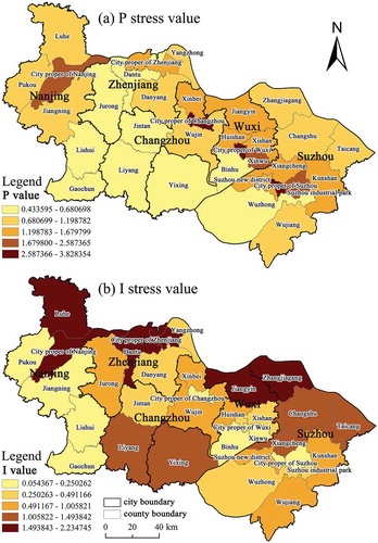
In 2015, the proportion of construction lands to the whole region is about 23.45%. City propers have the highest P stress values (especially Changzhou, Wuxi, and Suzhou) at about 85% greater and over 3.60 times the regional average value (Figure 3(a)). The units surrounding them follow (e.g., Suzhou Industrial Park and Xinwu), then come the units along the Yangtze river. Southern units are of lowest P values at about half the regional average value, including Liyang, Jintan, Jurong, where most of the region’s mountains and hills (including Mao and Yixing-Liyang Mountains) and large water bodies such as Taihu Lake are distributed.

Figure 3. P and I ecological stress values in Southern Jiangsu

I stress value of construction lands

The extent of I stress values was from 0.05 to 2.23, which is narrower than that of the P values (Supplementary Table 1). The spatial pattern of I stress values are also different with that of P stress values (Figure 3(b)). The units with highest I stress values are distributed along the Yangtze river including Luhe, Zhangjiagang, Jiangyin, and city propers of Zhenjiang and Nanjing, where the development of heavy industries has induced more environmental pollutants in the same amount of construction land. Most city propers have low I values, especially those far from Yangtze River, as heavy industries mostly move out after 2000. The spatial correlation of P and I values is not significant and no units contained highest levels of both values. However, there were some units with lowest levels of both P and I values: mountain regions or areas surrounding Taihu Lake, i.e., Lishui, Gaochun, and Binhu.

L stress value of construction lands

Ecological zoning based on EP simulation

Our MCR analysis indicates the expanding pattern of ecological space, which is similar to the irregular spread of contour lines. The spatial differentiation of raster resistance relating to different land-use types causes a deformation of concentric circles with ecological lands as the cores (Figure 4(a)). After reclassification, 10 ecological zones with different MCR values and ecological suitability account for 50.12%, 26.16%, 13.53%, 5.45%,2.13%, 1.17%, 0.76%, 0.40%, 0.20%, and 0.07% from the zones with highest to lowest ecological suitability (i.e., zones with lowest to highest MCR), respectively. The most-suitable zones (lowest MCR value) are of the highest share and mainly concentrate in areas surrounding Taihu Lake and Yangtze River as well as the Yixing-Liyang and Mao mountainous regions, which are closer to ecological lands and have low anthropogenic disturbance (Figure 4(b)). Ecological zones with low suitability are concentrated in urbanized areas including city propers of Nanjing, Suzhou, Wuxi, Changzhou, and also some regions close to the Shanghai metropolitan area, where there are large human populations and substantial economic agglomeration.

Figure 4. MCR value, ecological zones, ecological stress of construction lands and L stress value in Southern Jiangsu

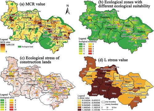
Spatial distribution of construction lands with different ecological stress

The overlay analysis of ecological zones and construction lands indicates that construction lands with 1–10 ecological stress values (i.e., those distributed at ecological zones with 1 to 10 ecological suitability) are 14.25, 59.81, 112.46, 206.69, 307.54, 517.35, 975.97, 1635.31, 1430.69, and 1358.28 km², respectively. The majority have high or mid-level ecological stress. Low-stress construction lands are mainly concentrated at the centers of prefecture cities (Nanjing, Suzhou, Wuxi, and Changzhou) and other developed county-level cities including Kunshan, Taicang, and Jiangyin (Figure 4(c)). These areas have low disturbance to regional ecological safety, and are hence suitable for population and industrial agglomeration.

Small patches of construction lands, mostly rural settlements, are of high ecological stress as they are distributed along Yangtze River, Taihu Lake, and eastern riverside or lakefront areas. Most of these areas were once wetlands or low mountains with high ecosystem services; the transformation to construction lands causes significant ecological disturbance. Some medium-sized cities also show middle-level ecological stress, where the construction lands are distributed in suburban areas and a transition from cultivated to construction lands is the main cause of ecological stress.

L stress value of different units

L stress values are significantly affected by the spatial distribution of construction lands and differ markedly from the P and I values (Figure 4(d)). Most units with high L values are located in the Mao and Yixing-Liyang mountainous areas, which have high ecological suitability. Construction lands in the ecologically suitable zones make the location effects significant. City propers are more suitable for land development and less suitable for ecological restoration, so their high amount of construction lands do not cause high ecological disturbance.

There are slight negative correlations between L and P values with Moran’s I = −0.2110 according to the multivariate LISA. The LISA also indicates a significant negative correlation in units with high L but low P values: Yixing, Liyang, Jintan, Lishui and Gaocun (Supplementary Table 1). The five units are all distributed at Mao Mountain and Yixing-Liyang Mountain. The spatial correlation of I and L values is not significant, indicating no overall spatial relationship between them.

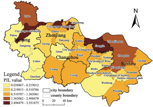
PIL stress values and dominant stressors for 33 units

After multiplication, the extent of PIL values ranges from 0.04 (Binhu, near Taihu Lake) to 3.55 (Jiangyin, along the Yangtze river). Spatially, all units with the highest levels of comprehensive ecological stress fall along the Yangtze, where I values are highest while P and L values are lower but not the lowest (Figure 5). The units with lowest PIL values are mostly located at mountainous areas or surrounding Taihu Lake such as Binhu and Gaochun. Interestingly, the city proper of Suzhou is at the lowest level (with PIL value 0.18). Although its P value is among the highest (3.76, just lower than city proper of Wuxi), the I and L values are both among the lowest (Supplementary Table 1).

Figure 5. PIL ecological stress value in Southern Jiangsu

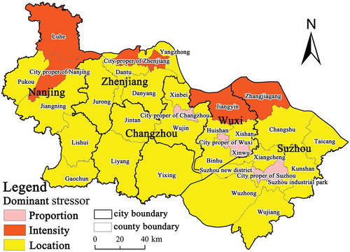
The effects of the proportion, intensity, and location of construction lands show significant spatial differentiation across the study region (Figure 6). Among the 33 units, 23 take location as the dominant stressors, suggesting an unreasonable spatial distribution of construction lands as the main driving force of ecological stress. The five units with land-use intensity as the dominant factor all lie along the Yangtze river, where massive pollutant emissions related to heavy industries are the major inducing factor. The five units with proportion as the dominant factor are mostly city propers or adjacent units where land development has been greatly promoted in recent years such as Xinwu and Suzhou Industrial Park.

Figure 6. Dominant stressors of the ecological stress in Southern Jiangsu

Discussion

As mentioned above, the ecological stress caused by land urbanization is affected by various attributes of construction lands which needs to be emphasized for providing comprehensive assessment. Here we chose three most common (and also most significant) attributes of land urbanization – the proportion, intensity, and location of construction lands – and designed targeted indicators to evaluate multi-perspective ecological stress. According to our analysis, the chosen attributes all have significant ecological effects, but the effects are spatially differentiated and with different dominance among 33 assessed units.

The proportion (or amount) of construction lands is the most direct attribute of land urbanization; a higher proportion means more natural spaces are occupied by construction lands which remits increased ecological stress (Imhoff et al. 2004; Lu et al. 2010; Peng et al. 2017). As a simplification, the proportion indicator is widely used to indicate the degree of ecological disturbance for the purposes of governmental land-use regulation policies (Fan et al. 2012; Liu et al. 2015). City propers have higher populations and economic agglomeration than surrounding areas; they have been developed over lengthy historical periods and have higher ecological stress than the surrounding areas as well. Units along the Yangtze river comprise high proportion effects in this study as they have been thoroughly industrially developed.

The proportion indicator does not emphasize the differences of the other attributes. The LUI indicator reflects the usage status of construction lands as per undesired outputs such as SO₂ and NO_x. Higher pollutant density induces more significant ecological stress due to certain construction lands. The spatial pattern of intensity is different from that of proportion in Southern Jiangsu; high-level units are mostly distributed along the Yangtze river, where heavy industries dominate the economic development. Luhe in Northern Nanjing is rife with steel, petrochemical, and electric power industrial projects. Large enterprises such as Sinopec Yangzi Petrochemical Co., Yangzi-BASF Petrochemical Co., Nanjing Chemical Industries Co., Nangang Iron & Steel United Co., and the Nanjing Power Plant lie along its riverside area. In 2015, the energy consumption of main industrial enterprises reached 21.79 million tons of standard coal accounting for 59.35% of Nanjing’s total; while its proportion of industrial output was just 11.34% of the whole value of Nanjing. Zhangjiagang is another important heavy industrial region where the No. 5 iron and steel enterprise in China (Jiangsu Shagang Group Co.) and also other similar industries (including Jiangsu Yonggang Group, Zhangjiagang Pohang Steel Group, etc.) are located in its metallurgical industrial park.

On the contrary, most city propers are at low levels as per the dominance of service-related and other urban industries. Although the proportion of construction lands are highest in city propers, their major industries are more environmentally friendly and emit less pollutants than heavy industries. To this effect, higher proportion stress does not necessarily mean more ecological stress – the stress effect is also related to the different functions of construction lands. Industrial development, especially the agglomeration of heavy industries, consumes more resources, emits more pollutants, and degrades the ecosystem more severely than other aspects of land urbanization.

The location effect is affected by both the spatial distribution of construction lands and the spatial heterogeneity of ecosystems (He et al. 2011; Li, Gao, and Chen 2019). Considering the importance of EP in maintaining ecosystem functions and services (Forman and Godron 1986; Wu and Yang. 2009), we carried out EP simulation to determine the spatial heterogeneity of ecological suitability via MCR model. Spaces surrounding certain sources/targets are of high ecological suitability while built-up areas of city propers are less suitable. Suitable ecological zones appear not only as patches, but also as corridors along the suitable landscape patches (Li et al. 2015; Li, Gao, and Chen 2019). Construction lands are located at different suitable zones and with different levels of ecological stress, so region-level location effects are also spatially differentiated as-evidenced by weighted analysis of the amount and stress values of construction lands in different units.

Basically, the location effects are more significant for units with more ecological spaces (e.g., mountains, hills, and water bodies) compared to proportion or intensity effects. Although these units have less construction lands, they are mostly ecologically suitable zones, especially some scattered rural settlements and other construction lands such as mines and traffic facilities (Li and Fan 2014). As scattered construction lands have strong ecological disturbance, it is recommended to promote moderately concentrated land development, repair damaged landscape structures, and restore ecological functions by reducing scattered construction lands and ecologically restoring existing ones (Sun et al. 2015; Shi et al. 2018). As the ecological stress of construction lands are identified in this study based on EP simulation and related ecological zoning, the ecological restoration of construction lands as-identified here is important not only to protect ecological spaces but also to maintain potential EP and related functions (Li, Gao, and Chen 2019).

The spatial patterns of proportion, intensity, and location effects in terms of the ecological stress of construction lands differ markedly considering their various perspectives and indicators. The proportion effect is higher in city propers where construction lands are highly concentrated, while the intensity effect is more significant in units along the Yangtze river where heavy industries are gathered. Ecologically suitable units have higher location effect, where the conflicts between land development and ecological protection often happen. The effects of proportion, intensity, and location are indeed spatially differentiated but only proportion and location are negatively correlated. After combining the three indicators, the comprehensive effects are quite different from the single-perspective effects. Units with at least two high indicators tend to show high or low comprehensive effects accordingly, such as the city propers of Nanjing and Zhenjiang (two high-level indicators) and Gaochun and Lishui (two low-level indicators). The comprehensive values of most units are predicted differently as their single-perspective values are quite different, and the relationships among them are highly complex.

The identification of dominant stressors makes clearer the spatially differentiated effect of proportion, intensity, and location. Basically, the ecological stress of most units can be attributed to an unreasonable distribution of construction lands, especially in suburban units or areas far from city propers. Besides, few units are mainly affected by high proportion and intensity of construction lands, which are most city propers or cities along the Yangtze river. In land-use planning, although it is all important to control the proportion, improve the efficiency and optimize the spatial distribution, targeted measures should be spatially different according to specific conditions. The identification of dominant stressors facilitates the proposal of specific planning suggestions. For those with location as the dominant stressors, it is primary to promote the spatial optimization of land development (He et al. 2011; Liu, Fang, and Li 2014). To be specific, existing construction lands in zones with high ecological suitability should be ecologically restored; while future land development should be restricted to ecological zones with lower ecological suitability. In units with proportion as the dominant factor, it is necessary to strictly control the amount of construction lands and conserve more green spaces through targeted urban land management activities (Zhou et al. 2014; Liu et al. 2015). Units with intensity as the dominant factor are mostly characterized by high-pollution heavy industries, and it is prior to optimize the economic structure and promote environmentally friendly industries (e.g., modern tertiary industries) or make existing industries greener (Jänicke 2008). On the whole, further land development may be encouraged in regions with low ecological suitability by controlling the total quantity and improving utilization efficiency (Li, Gao, and Chen 2019).

Conclusion

It is the prerequisite to coordinate the reship between land urbanization and ecological protection by understanding what the ecological effects are during rapid land urbanization comprehensively. Here we carried out corresponding analysis from the perspectives of the proportion, intensity, and location of construction lands, and results indicated a comprehensive evaluation could better objectively reflect the ecological effects of land urbanization and the expansion of construction lands than single-perspective assessments. The induced ecological stress of different attributes differs significantly as per their degree and spatial differentiation. Accordingly, targeted measures should be proposed based on dominant stressors to improving their efficiency.

It is obviously an over-generalization to ascribe the ecological effects of construction lands to their proportion, intensity, and location – there are other attributes such as the various types of constructions lands, the different effects of economic activities, and the diversity in population structures and lifestyles. Further research is yet needed to complete a fully precise assessment and to determine effective targeted measures accordingly.

Acknowledgments

We thank RESDC for providing land-use data in 2015, and the China Scholarship Council for providing financial support. In addition, we are grateful to the editors and the anonymous reviewers for exceptionally helpful comments and suggestions.

Disclosure statement

No potential conflict of interest was reported by the authors.

Supplementary material

Supplemental data for this article can be accessed here.

Additional information

Funding

The work was sponsored by the National Natural Science Foundation of China (41871209, 41701193 and 41401187).

References

- Adriaensen, F., J. P. Chardon, G. De Blust, E. Swinnen, S. Villalba, H. Gulinck, and E. Matthysen. 2003. “The Application of ‘least-cost’ Modelling as a Functional Landscape Model.” Landscape and Urban Planning 64 (4): 233–247. doi:10.1016/S0169-2046(02)00242-6.
- Blasi, C., M. Marignani, R. Copiz, M. Fipaldini, S. Bonacquisti, E. Del Vico, L. Rosati, and L. Zavattero. 2011. “Important Plant Areas in Italy: From Data to Mapping.” Biological Conservation 144 (1): 220–226. doi:10.1016/j.biocon.2010.08.019.
- Brown, M. T., and K. C. Reiss. 2010. “Landscape Development Intensity and Pollutant Emergy/EMpower Density Indices as Indicators of Ecosystem Health.” In Handbook of Ecological Indicators for Assessment of Ecosystem Health (2nd ed.), edited by S. E. Jørgensen, F. L. Xu, and R. Costanza, 171–188. New York: CRC Press.
- Buttel, F. H. 2000. “Ecological Modernization as Social Theory.” Geoforum 31 (1): 57–65. doi:10.1016/S0016-7185(99)00044-5.
- Carlier, J., and J. Moran. 2019. “Landscape Typology and Ecological Connectivity Assessment to Inform Greenway Design.” Science of the Total Environment 651: 3241–3252. doi:10.1016/j.scitotenv.2018.10.077.
- Chen, J. Q., R. X. Chu, H. Wang, L. C. Zhang, X. D. Chen, and Y. F. Du. 2019. “Alleviating Urban Heat Island Effect Using High-conductivity Permeable Concrete Pavement.” Journal of Cleaner Production 237: 117722. doi:10.1016/j.jclepro.2019.117722.
- Cherniwchan, J. 2012. “Economic Growth, Industrialization, and the Environment.” Resource and Energy Economics 34 (4): 442–467. doi:10.1016/j.reseneeco.2012.04.004.
- Dadashpoor, H., P. Azizi, and M. Moghadasi. 2019. “Land Use Change, Urbanization, and Change in Landscape Pattern in a Metropolitan Area.” Science of the Total Environment 655: 707–719. doi:10.1016/j.scitotenv.2018.11.267.
- Daily, G. C. 1997. Nature’s Services: Societal Dependence on Natural Ecosystems. Washington: Island Press.
- Dupras, J., J. Marull, L. Parcerisas, F. Coll, A. Gonzalez, M. Girard, and E. Tello. 2016. “The Impacts of Urban Sprawl on Ecological Connectivity in the Montreal Metropolitan Region.” Environmental Science & Policy 58: 61–73. doi:10.1016/j.envsci.2016.01.005.
- Ellis, E. C., and N. Ramankutty. 2008. “Putting People in the Map: Anthropogenic Biomes of the World.” Frontiers in Ecology and the Environment 6 (8): 439–447. doi:10.1890/070062.
- Erb, K. H., H. Haberl, and M. Rudbeck. 2013. “A Conceptual Framework for Analysing and Measuring Land-use Intensity.” Current Opinion in Environmental Sustainability 5 (5): 464–470. doi:10.1016/j.cosust.2013.07.010.
- Estoque, R. C., and Y. Murayama. 2016. “Quantifying Landscape Pattern and Ecosystem Service Value Changes in Four Rapidly Urbanizing Hill Stations of Southeast Asia.” Landscape Ecology 31 (7): 1481–1507. doi:10.1007/s10980-016-0341-6.
- Fan, J., W. Sun, K. Zhou, and D. Chen. 2012. “Major Function Oriented Zone: New Method of Spatial Regulation for Reshaping Regional Development Pattern in China.” Chinese Geographical Sciences 22: 196–209. doi:10.1007/s11769-012-0528-y.
- Feng, J., J. Yan, Z. Yu, X. Zeng, and W. Xu. 2018. “Case Study of an Industrial Park toward Zero Carbon Emission.” Applied Energy 209: 65–78. doi:10.1016/j.apenergy.2017.10.069.
- Ferreras, P. 2001. “Landscape Structure and Asymmetrical Inter-patch Connectivity in a Metapopulation of the Endangered Iberian Lynx.” Biological Conservation 100: 125–136. doi:10.1016/S0006-3207(00)00213-5.
- Forman, R. T. T., and M. Godron. 1986. Landscape Ecology. New York, NY: John Wiley & Sons.
- Gong, J., W. Chen, Y. Liu, and J. Wang. 2014. “The Intensity Change of Urban Development Land: Implications for the City Master Plan of Guangzhou, China.” Land Use Policy 40: 91–100. doi:10.1016/j.landusepol.2013.05.001.
- Gonzalez, J. R., G. Del Barrio, and B. Duguy. 2008. “Assessing Functional Landscape Connectivity for Disturbance Propagation on Regional scales-A Cost-Surface Model Approach Applied to Surface Fire Spread.” Ecological Modeling 211 (1–2): 121–141. doi:10.1016/j.ecolmodel.2007.08.028.
- Grimm, N. B., S. H. Faeth, N. E. Golubiewski, C. L. Redman, J. Wu, X. Bai, and J. M. Briggs. 2008. “Global Change and the Ecology of Cities.” Science 319 (5864): 756–760. doi:10.1126/science.1150195.
- Grossman, M., and A. B. Krueger. 1995. “Economic Growth and the Environment.” Quarterly Journal of Economics 110 (2): 353–377. doi:10.3386/w4634.
- He, C., J. Tian, P. Shi, and D. Hu. 2011. “Simulation of the Spatial Stress Due to Urban Expansion on the Wetlands in Beijing, China Using a GIS-based Assessment Model.” Landscape and Urban Planning 101: 269–277. doi:10.1016/j.landurbplan.2011.02.032.
- Horvath, Z., R. Ptacnik, C. F. Vad, F. Csaba, and J. M. Chase. 2019. “Habitat Loss over Six Decades Accelerates Regional and Local Biodiversity Loss via Changing Landscape Connectance.” Ecology Letters 22 (6): 1019–1027. doi:10.1111/ele.13260.
- Huang, L., J. Han, K. Yuan, and W. Xiang. 2016. “Analysis of the Built-up Area’s Carbon Emission Intensity and Its Regional Disparity in China.” Environmental Science & Technology 39: 185–191. (in Chinese).
- Imhoff, M. L., L. Bounoua, R. DeFries, W. T. Lawrence, D. Stutzer, C. J. Tucker, and T. Ricketts. 2004. “The Consequences of Urban Land Transformation on Net Primary Productivity in the United States.” Remote Sensing of Environment 89: 434–443. doi:10.1016/j.rse.2003.10.015.
- Imhoff, M. L., W. T. Lawrence, C. D. Elvidge, T. Paul, E. Levine, M. V. Privalsky, and V. Brown. 1997. “Using Nighttime DMSP/OLS Images of City Lights to Estimate the Impact of Urban Land Use on Soil Resources in the United States.” Remote Sensing of Environment 59 (1): 105–117. doi:10.1016/S0034-4257(96)00110-1.
- Irankhahi, M., S. A. Jozi, P. Farshchi, S. M. Shariat, and H. Liaghati. 2017. “Combination of GISFM and TOPSIS to Evaluation of Urban Environment Carrying Capacity (Case Study: Shemiran City, iran).” International Journal of Environmental Science and Technology 14 (6): 1317–1332. doi:10.1007/s13762-017-1243-0.
- Jackson, S. F., K. Walker, and K. J. Gaston. 2009. “Relationship between Distributions of Threatened Plants and Protected Areas in Britain.” Biological Conservation 142 (7): 1515–1522. doi:10.1016/j.biocon.2009.02.020.
- Jänicke, M. 2008. “Ecological Modernisation: New Perspectives.” Journal of Cleaner Production 16: 557–565. doi:10.1016/j.jclepro.2007.02.011.
- Jiang, L., X. Z. Deng, and K. C. Seto. 2013. “The Impact of Urban Expansion on Agricultural Land Use Intensity in China.” Land Use Policy 35: 33–39. doi:10.1016/j.landusepol.2013.04.011.
- Knappen, J. P., M. Scheffer, and B. Harms. 1992. “Estimating Habitat Isolation in Landscape Planning.” Landscape and Urban Planning 23: 1–16. doi:10.1016/0169-2046(92)90060-D.
- Lambin, E. F., M. D. A. Rounsevell, and H. J. Geist. 2000. “Are Agricultural Land-use Models Able to Predict Changes in Land-use Intensity?” Agriculture, Ecosystems & Environment 82 (1–3): 321–331. doi:10.1016/S0167-8809(00)00235-8.
- Lambin, E. F., B. L. Turner, H. J. Geist, S. B. Agbola, A. Angelsen, J. W. Bruce, O. T. Coomes, et al. 2001. “The Causes of Land-use and Land-cover Change: Moving beyond the Myths.” Global Environmental Change 11: 261–269. doi:10.1016/S0959-3780(01)00007-3.
- Li, F., Y. Ye, B. Song, and R. Wang. 2015. “Evaluation of Urban Suitable Ecological Land Based on the Minimum Cumulative Resistance Model: A Case Study from Changzhou, China.” Ecological Modeling 318: 194–203. doi:10.1016/j.ecolmodel.2014.09.002.
- Li, P., D. Chen, and J. Fan. 2011. “Research of Ecological Occupiability Based on Least-cost Distance Model: A Case Study on Xijiang River Economic Belt in Guangxi.” Journal of Natural Resources 26(2): 227–236. (in Chinese).
- Li, P., and J. Fan. 2014. “Regional Ecological Vulnerability Assessment of the Guangxi Xijiang River Economic Belt in Southwest China with VSD Model.” Journal of Resources and Ecology 5 (2): 163–170. doi:10.5814/j.issn.1674-764X.2014.02.009.
- Li, P., J. Gao, and J. Chen. 2019. “Quantitative Assessment of Ecological Stress of Construction Lands by Quantity and Location: Case Study in Southern Jiangsu, Eastern China.” Environment, Development and Sustainability. doi:10.1007/s10668-018-0262-4.
- Liu, X., J. Shu, and L. Zhang. 2010. “Research on Applying Minimal Cumulative Resistance Model in Urban Land Ecological Suitability Assessment: As an Example of Xiamen City.” Acta Ecologica Sinica 30(2): 421–428. (in Chinese).
- Liu, Y., F. Fang, and Y. Li. 2014. “Key Issues of Land Use in China and Implications for Policy Making.” Land Use Policy 40: 6–12. doi:10.1016/j.landusepol.2013.03.013.
- Liu, Y., Y. Wang, J. Peng, and Y. Du. 2015. “Correlations between Urbanization and Vegetation Degradation across the World’s Metropolises Using DMSP/OLS Nighttime Light Data.” Remote Sensing 7: 2067–2088. doi:10.3390/rs70202067.
- Long, H. L., Y. Q. Liu, X. G. Hou, T. Li, and Y. Li. 2014. “Effects of Land Use Transitions Due to Rapid Urbanization on Ecosystem Services: Implications for Urban Planning in the New Developing Area of China.” Habitat International 44: 536–544. doi:10.1016/j.habitatint.2014.10.011.
- Lu, D., X. Xu, H. Tian, E. Moran, M. Zhao, and S. Running. 2010. “The Effects of Urbanization on Net Primary Productivity in Southeastern China.” Environmental Management 46: 404–410. doi:10.1007/s00267-010-9542-y.
- Marignani, M., and C. Blasi. 2012. “Looking for Important Plant Areas: Selection Based on Criteria, Complementarity, or Both?” Biodiversity Conservation 21 (7): 1853–1864. doi:10.1007/s10531-012-0283-5.
- Nguyen, A. K., Y. Liou, M. Li, and T. A. Tran. 2016. “Zoning Eco-Environmental Vulnerability for Environmental Management and Protection.” Ecological Indicators 69: 100–117. doi:10.1016/j.ecolind.2016.03.026.
- Ning, J., J. Liu, W. Kuang, X. Xu, S. Zhang, C. Yan, R. Li, et al. 2018. “Spatiotemporal Patterns and Characteristics of Land-use Change in China during 2010 – 2015.” Journal of Geographical Sciences 28 (5): 547–562. doi:10.1007/s11442-018-1490-0.
- Peng, J., L. Tian, Y. Liu, M. Zhao, Y. Hu, and J. Wu. 2017. “Ecosystem Services Response to Urbanization in Metropolitan Areas: Thresholds Identification.” Science of the Total Environment 607–608: 706–714. doi:10.1016/j.scitotenv.2017.06.218.
- Sakieh, Y., B. J. Amiri, A. Danekar, J. Feghhi, and S. Dezhkam. 2015. “Scenario-based Evaluation of Urban Development Sustainability: An Integrative Modeling Approach to Compromise between Urbanization Suitability Index and Landscape Pattern.” Environment, Development and Sustainability 17 (6): 1343–1365. doi:10.1007/s10668-014-9609-7.
- Saunders, W. S. A., and J. S. Becker. 2015. “A Discussion of Resilience and Sustainability: Land Use Planning Recovery from the Canterbury Earthquake Sequence, New Zealand.” International Journal of Disaster Risk Reduction 14: 73–81. doi:10.1016/j.ijdrr.2015.01.013.
- Schadt, S., F. Knauer, P. Kaczensky, E. Revilla, T. Wiegand, and L. Trepl. 2002. “Rule-based Assessment of Suitable Habitat and Patch Connectivity for Eurasian Lynx in Germany.” Ecological Application 12: 1469–1483. doi:10.1890/1051-0761(2002)012.
- Seto, K. C., B. Güneralp, and L. R. Hutyrac. 2012. “Global Forecasts of Urban Expansion to 2030 and Direct Impacts on Biodiversity and Carbon Pools.” PNAS 109 (40): 16083–16088. doi:10.1073/pnas.1211658109.
- Shi, B. Q., P. M. Bach, A. Lintern, K. F. Zhang, R. A. Coleman, L. Metzeling, D. T. McCarthy, and A. Deletic. 2019. “Understanding Spatiotemporal Variability of In-stream Water Quality in Urban Environments - A Case Study of Melbourne, Australia.” Journal of Environmental Management 246: 203–213. doi:10.1016/j.jenvman.2019.06.006.
- Shi, Y., X. Cao, D. Fu, and Y. Wang. 2018. “Comprehensive Value Discovery of Land Consolidation Projects: An Empirical Analysis of Shanghai, China.” Sustainability 10: 2039. doi:10.3390/su10062039.
- Sieber, J., and M. Pons. 2015. “A Assessment of Urban Ecosystem Services Using Ecosystem Services Reviews and GIS-based Tools.” Procedia Engineering 115: 53–60. doi:10.1016/j.proeng.2015.07.354.
- Su, H. D., X. Cao, D. C. Wang, Y. W. Jia, G. Ni, J. Wang, M. Zhang, and C. Niu. 2019. “Estimation of Urbanization Impacts on Local Weather: A Case Study in Northern China (Jing-jin-ji district).” Water 11: 797. doi:10.3390/w11040797.
- Su, Y., X. Chen, J. Liao, H. Zhang, C. Wang, Y. Ye, and Y. Wang. 2016. “Modeling the Optimal Ecological Security Pattern for Guiding the Urban Constructed Land Expansions.” Urban Forestry and Urban Greening 19: 35–46. doi:10.1016/j.ufug.2016.06.013.
- Sun, X., S. Xiong, X. Zhu, X. Zhu, Y. Li, and B. L. Li. 2015. “A New Indices System for Evaluating Ecological-economic-social Performances of Wetland Restorations and Its Application to Taihu Lake Basin, China.” Ecological Modeling 295: 216–226. doi:10.1016/j.ecolmodel.2014.10.008.
- Tian, L., J. Chen, and S. X. Yu. 2014. “Coupled Dynamics of Urban Landscape Pattern and Socioeconomic Drivers in Shenzhen, China.” Landscape Ecology 29 (4): 715–727. doi:10.1007/s10980-014-9995-0.
- Turner, II, B. L., and W. E. Doolittle. 1978. “The Concept and Measure of Agricultural Intensity.” Professional Geographer 30 (3): 297–301. doi:10.1111/j.0033-0124.1978.00297.x.
- Turner, II, B. L., W. C. Clark, R. W. Kates, J. F. Richards, J. T. Mathews, and W. B. Meyer, Eds. 1990. The Earth as Transformed by Human Action: Global and Regional Changes in the Biosphere over the past 300 Years. Cambridge: Cambridge University Press.
- van Diggelen, R., F. J. Sijtsma, D. Strijker, and J. van den Burga. 2005. “Relating Land-use Intensity and Biodiversity at the Regional Scale.” Basic and Applied Ecology 6: 145–159. doi:10.1016/j.baae.2005.01.004.
- Villalba, S., H. Gulinck, G. Verbeylen, and E. Matthysen. 1998. “Relationship between Patch Connectivity and the Occurrence of the European Red Squirrel, Sciurus Vulgaris, in Forest Fragments within Heterogeneous Landscapes.” In Key Concepts in Landscape Ecology, edited by J. W. Dover and R. G. H. Bunce, 205–220. UK: IALE, Preston.
- Wang, J., T. Zhai, Y. Lin, X. Kong, and T. He. 2019. “Spatial Imbalance and Changes in Supply and Demand of Ecosystem.” Science of the Total Environment 657: 781–791. doi:10.1016/j.scitotenv.2018.12.080.
- Wu, J., and J. Yang., eds. 2009 Lectures in Modern Ecology (IV): Theory and Applications. Beijing: Higher Education Press. (in Chinese).
- Xiang, Y., and J. Meng. 2016. “Research into Ecological Suitability Zoning and Expansion Patterns in Agricultural Oases Based on the Landscape Process: A Case Study in the Middle Reaches of the Heihe River.” Environmental Earth Sciences 75: 1355. doi:10.1007/s12665-016-6165-5.
- Xie, H., Q. Zhai, W. Wang, J. Yu, F. Lu, and Q. Chen. 2018. “Does Intensive Land Use Promote a Reduction in Carbon Emissions? Evidence from the Chinese Industrial Sector.” Resources, Conservation and Recycling 137: 167–176. doi:10.1016/j.resconrec.2018.06.009.
- Xu, H., Y. Guo, and Z. Chen. 2013. “The Relationship between Land Market Development, Urban Land Intensive Use and Carbon Emission: An Empirical Study Based on Provincial Panel Data in China.” China Land Science 27: 26–29. (in Chinese).
- Ye, Y., Y. Su, H. Zhang, K. Liu, and Q. Wu. 2015. “Construction of an Ecological Resistance Surface Model and Its Application in Urban Expansion Simulations.” Journal of Geographical Sciences 25 (2): 211–224. doi:10.1007/s11442-015-1163-1.
- Yu, K. 1996. “Security Patterns and Surface Model in Landscape Ecological Planning.” Landscape and Urban Planning 36 (1): 1–17. doi:10.1016/S0169-2046(96)00331-3.
- Zampella, R. A., N. A. Procopio, R. G. Lathrop, and C. L. Dow. 2007. “Relationship of Land use/land Cover Patterns and Surface Water Quality in the Mullica River Basin.” Journal of the American Water Resources Association 43: 594–604. doi:10.1111/j.1752-1688.2007.00045.x.
- Zhang, J., A. Zhang, and J. Dong. 2013. “Study on Relationship of Intensive Land Use and Carbon Emission—A Case Study of Wuhan Urban Agglomeration.” Research on Agricultural Modernization 34(6): 717–721. (in Chinese.
- Zhao, S., L. Da, Z. Tang, H. Fang, K. Song, and J. Fang. 2006. “Ecological Consequences of Rapid Urban Expansion: Shanghai, China.” Frontiers in Ecology and the Environment 4 (7): 341–346. doi:10.1890/1540-9295(2006)004[0341:ECORUE]2.0.CO;2.
- Zhao, S., D. Zhou, C. Zhu, W. Qu, J. Zhao, Y. Sun, D. Huang, W. Wu, and S. Liu. 2015. “Rates and Patterns of Urban Expansion in China’s 32 Major Cities over the past Three Decades.” Landscape Ecology 30: 1541–1559. doi:10.1007/s10980-015-0211-7.
- Zhong, T., Y. Chen, and X. Huang. 2016. “Impact of Land Revenue on the Urban Land Growth toward Decreasing Population Density in Jiangsu Province, China.” Habitat International 58: 34–41. doi:10.1016/j.habitatint.2016.09.005.
- Zhou, D., S. Zhao, S. Liu, and L. Zhang. 2014. “Spatiotemporal Trends of Terrestrial Vegetation Activity along the Urban Development Intensity Gradient in China’s 32 Major Cities.” Science of the Total Environment 488: 136–145. doi:10.1016/j.scitotenv.2014.04.080.
- Zhu, X., P. Zhang, Y. Wei, Y. Li, and H. Zhao. 2019. “Measuring the Efficiency and Driving Factors of Urban Land Use Based on the DEA Method and the PLS-SEM model—A Case Study of 35 Large and Medium-sized Cities in China.” Sustainable Cities and Society 50: 101646. doi:10.1016/j.scs.2019.101646.