A global analysis of CO₂ and non-CO₂ GHG emissions embodied in trade with Belt and Road Initiative countries

ABSTRACT

Introduction: The Belt and Road Initiative (BRI) is an important cooperative framework that increasingly affects the global economy, trade, and emission patterns. However, most existing studies pay insufficient attention to consumption-based emissions, embodied emissions, and non-CO2 greenhouse gases (GHGs). This study constructs a GHG emissions database to study the trends and variations in production-based, consumption-based, and embodied emissions associated with BRI countries.Outcome: We find that the per capita GHG emissions of BRI countries are lower than the global average but show significant variation within this group. We also find that trade-embodied emissions between BRI countries and China are growing. As a group, BRI countries are anet exporter of GHGs, with a global share of net export emissions of about 20%. In 2011, nearly 80% of GHG export emissions from BRI countries flowed to non-BRI countries, and nearly 15% flowed to China; about 57% of GHG import emissions were from non-BRI countries, and about 38% were from China.Conclusion: Therefore, this study concludes that the BRI should be used to coordinate climate governance to accelerate and strengthen the dissemination and deployment of low-emissions technologies, strategies, and policies within the BRI so as to avoid a carbon-intensive lock-in effect.

KEYWORDS:

• Belt and Road Initiative (BRI)
• China
• consumption-based emissions
• non-CO₂ greenhouse gas (NCO₂)
• embodied emissions
• global multi-regional input-output model (MRIO)

Introduction

Inherited and developed from the ancient Silk Road, the Belt and Road Initiative (BRI) was launched by China in 2013 (Ma and Zadek 2019). Policy coordination, infrastructure connectivity, unimpeded trade, financial integration, and cultural communication are described as the five key aspects of improving regional connectivity in the long term, among which trade is the central focus of the BRI. As a China-backed global cooperation initiative that could provide unparalleled international economic cooperation opportunities, BRI quickly expanded to 138¹ countries within 6 years, distributed across Asia, Europe, Africa, Oceania, and Latin America. Country types engaged in BRI are mainly emerging economies, oil-exporting countries, and areas lacking resources such as small island states (Chen et al. 2020). They represent about 70% of the global developing and least developed countries and 90% of the population in the groups that are still at a relatively low-income development stage.

Undoubtedly, BRI is increasingly affecting and even reshaping the global economy, trade, and emission patterns, as well as global climate change. On the one hand, the BRI cooperation framework could spur a sharp acceleration in economic growth and development across these economies, especially in poverty-stricken areas within the BRI. On the other hand, by establishing a network of various investments in infrastructure – including roads, railways, airports, ports, power stations, pipelines, and IT networks to link China with participating economies (Huang 2019), the BRI could also cause a wide range of potential environmental and climate consequences which might constitute a challenge to achieving the objectives of the Paris Agreement (Ascensão et al. 2018; Hughes et al. 2020; Ning et al. 2017; Teo et al. 2019; Yang, Flower, and Thompson 2019; Zhang et al. 2019a). As a whole, BRI countries currently account for roughly 30% of global greenhouse gas (GHG) emissions, with more than 40% of the population and 20% of global GDP. Although most BRI countries contributed much less than the global average to historical and cumulative GHG emissions, many scholars agree that the BRI’s potential impact on both economic growth and GHG emissions in the future will be significant (Chen et al. 2020; Huang 2019; Ma and Zadek 2019).

In terms of emissions, the BRI countries are a much more complex system than any single country or even multinational economy like the European Union (EU) due to major differences in ecological environment characteristics, resource endowments, economic development level, and capacity for tackling climate change. Meanwhile, taking investment across BRI and trade globally as central focuses, BRI countries have more frequent import and export activities than in the past, leading to the complex emission accounting problems (Chen et al. 2020; Wu et al. 2020).

The GHG emissions accounting problems embedded in global trade and cooperation have received more attention within the last two decades, long before the BRI was announced. After the Kyoto Protocol was enacted in 1997, the definition of carbon emissions responsibility caused much dispute among countries. If environmental responsibility is defined only through producer responsibility, the spatial difference between production and consumption resulting from cross-border trade, which in nature is an emissions transfer, would be ignored (Davis and Caldeira 2010; Peters and Hertwich 2008). It was argued that the GHG emissions of all countries and regions should be accounted based on “consumer responsibility” (Peters 2008). The consumption-based accounting principle includes emissions from all end-use products consumed in a country, including final consumption, capital formation, and imports. About one-fourth to one-third of global GHG emissions are embodied in international trade (Davis and Caldeira 2010; Peters and Hertwich 2008; Peters et al. 2011), leaving significant differences between production- and consumption-based emissions in different countries. The IPCC’s Fifth Assessment Report underlined that the consumption-based approach is an important supportive means in establishing national emission inventories as well as in determining the emissions embedded in trade (IPCC 2014; Wu et al. 2020)

From the perspective of consumption-based and embodied emissions, many BRI countries’ production-based emissions are significantly higher than their consumption-based ones, making them net exporters of embodied emissions, with emissions exporting mostly to developed countries (Han et al. 2018; Peters and Hertwich 2008). According to research, the majority of production and supply in international trade occurs in developing countries, whereas developed countries take the roles of importers and net consumers (Davis and Caldeira 2010; Li et al. 2018; Peters and Hertwich 2008; Wood et al. 2019). Taking the year of 2004 as an example, China was then the largest net exporter of embodied emissions, accounting for 22.5% of its total GHG production-based emissions. China’s embodied emissions level was followed by Russia, the Middle East, South Africa, Uruguay, India, Southeast Asia, Eastern Europe, and South America, which make up most of the developing countries within the BRI framework now. The largest net importers of embodied emissions are the US., Japan, the UK, Germany, and France, which are all developed countries outside of the BRI framework (Davis and Caldeira 2010).

Although the consumption-based emissions of BRI countries have been extensively studied, most existing BRI-related studies cover only a few key BRI countries, and seldom take into account the internal differences among the BRI countries. In addition, they mostly focus on CO₂ or total GHGs while ignoring the specific emissions of non-CO₂ (NCO₂) GHGs, which have a strong greenhouse effect but also a large reduction potential. To close this gap, by taking a group of 88 BRI countries (BRI-88) as the study objective, this paper contributes to existing literature by not only calculating BRI’s total GHG production-based emissions, consumption-based emissions, and emissions embodied in trade, but also analyzing the flow pattern and sector distribution of four specific gases (CO2, CH4, N2O, and Fgas).

The rest of the paper is organized as follows. Section 2 reviews the related literature. Section 3 introduces the methodology and data used in this paper. Section 4 describes the calculation results. Section 5 summarizes the main conclusions and puts forward policy implications.

Literature review

Several studies have begun to use different analytical tools to assess the GHG emissions associated with the BRI. Panel data on Belt and Road countries have allowed researchers to explore the relationship between globalization and CO₂ emissions (Rauf et al. 2020; Saud et al. 2020; Zhang, Jin, and Shen 2018), generally finding an environmental Kuznets curve-type relationship between increased investment and trade and environmental impacts (Muhammad et al. 2020; Rauf et al. 2018). Although energy consumption and emissions in BRI countries are rising over time, both in absolute terms and in terms of intensity, China is on a path to achieving its emissions intensity targets (Fan et al. 2019). This leads to potential transfer of emissions through trade, further highlighting the importance of our research for characterizing the growing trade between China and BRI countries in terms of embodied emissions.

Since consumption-based and embodied emissions in trade have been extensively studied (Hung, Hsu, and Cheng 2019; Mendelsohn 2010; Sakai and Barrett 2016; Tamiotti et al. 2009), many methodological approaches have been developed, such as Material Flow Analysis (MFA) and Input–Output Analysis (IOA). The two methods have different system boundaries and data scope. MFA always focuses on direct trade between regions or countries (Hubacek and Feng 2016), pursues detailed commodity-level data, and takes into account non-market flows (Schaffartzik, Wiedenhofer, and Eisenmenger 2015; Taherzadeh and Caro 2019). Therefore, it is useful for analyzing the flow of a certain good or service, such as agricultural products or minerals (Brunner and Rechberger 2004; Liu et al. 2019; Ohno et al. 2016; Taherzadeh and Caro 2019).

Unlike MFA, IOA takes a supply chain at the global and multi-sector level as the system boundary (Hubacek and Feng 2016) and considers the direct and indirect material requirements and emissions in trade (Weisz and Duchin 2006). In early studies, the single-region input–output (SRIO) model was used to calculate the transfer of emissions within a single country. It was assumed that domestic and foreign products have the same production technology, which ignored the difference in energy structures and emissions coefficients, and thus skewed the calculations (Lenzen, Pade, and Munksgaard 2010). Upon the emergence of global databases such as the Global Trade Analysis Project (GTAP) Database and the World Input–Output Database (WIOD), the multi-regional input-output (MRIO) model, which can distinguish different production technologies, resource uses, and emission intensities in multiple countries and sectors, made it possible to track global emissions flows and to calculate consumption-based emissions and embodied emissions (Andrew and Peters 2013; Hertwich 2005; Peters 2007; Peters and Hertwich 2006; Wiedmann 2009).

Combining the MRIO method with the WIOD database, Wang, Z. et al. found that the main destinations of CO₂ export emissions from India are developed countries, whereas the main sources of import emissions are developing countries (Wang et al. 2018). Wang, X. et al. used the MRIO model and the GTAP database to study the consumption-based emissions of Kazakhstan and found that Russia and China are the major consumers of its emissions (Wang et al. 2019). By using MRIO, Meng et al. found that from 2004 to 2011, carbon flows among China, India, the Middle East and North Africa, and other Asia-Pacific regions increased. These findings indicated strong growth of emissions related to south–south trade (Meng et al. 2018). From this, we can see that the global trade landscape has changed since developing countries like China and India have become more involved, and the center of trade-related emissions has shifted from Europe to Asia (Zhang et al. 2019b).

BRI has provided strong support for trade and investment for developing countries (Meng et al. 2018), and some studies have preliminarily explored BRI carbon emissions using the above methods. Ding et al. used the SRIO and WIOD database to study the carbon flow of China and 68 BRI countries and 38 non-BRI countries (including the US, Canada, and Japan, etc.). They found that the proportion of China’s export emissions to BRI countries increases from 20.4% to 35.8%, and that the import emissions also continue to grow and exceeds the imports from non-BRI countries in their model in 2011 (Ding, Ning, and Zhang 2018). Han et al. combined the MRIO and Eora database and found that over 95% of the global net embodied carbon exports originate from BRI regions. Apart from Southeast Asia and some Central European countries, the carbon intensity of BRI production is significantly higher than that of consumption; 83.06% of the carbon emissions from production are used for intra-regional consumption, and the rest flows to the US, Western Europe, and other regions (Han et al. 2018). Cai et al. calculated the import and export carbon emissions flows between 64 BRI countries and China using MRIO analysis. China was found to be the pollution haven for 22 developed countries, whereas 19 developing countries have become pollution havens for China (Cai et al. 2018). As a trade-transit country, China has primarily exchanged trade deficits for CO₂ reduction in the Sino-Russian trade, and CO₂ emissions for trade surplus in the Sino-Indian trade. In the Sino-Brazil trade, both net exports of CO₂ emissions and trade deficits exist (Pan and Wei 2015; Zhang et al. 2019c).

Compared with CO₂, NCO₂ GHGs have stronger greenhouse effects and are also worthy of attention (Breidenich et al. 1998), but very little research on BRI emissions includes NCO₂ GHGs. NCO₂ primarily includes CH₄, N₂O, and fluorine-containing gases (Fgas), accounting for about 25% of global GHG emissions. NCO₂ emissions significantly differ from CO₂ emissions at the sectoral and regional levels. As an important GHG component, the impact of NCO₂ on climate change should not be underestimated and instead should be integrated into the global GHG emissions’ accounting system for overall consideration. However, only a handful of earlier studies from a global perspective have considered total GHG emissions. For instance, based on the MRIO and GTAP database, Hertwich et al. found that NCO₂ (including CH₄, N₂O, and Fgas) emissions account for nearly one-third of the total GHG emissions in the world (Hertwich and Peters 2009). International trade also affects NCO₂ emissions. Zhang et al. found that the embodied emissions of CH₄ in international trade accounts for 49.5% of the total global production-based CH₄ emissions, which is a much higher share than for CO2 emissions. The US, Japan, and some Western European countries are important net importers of CH₄, whereas China, sub-Saharan Africa, and India are important net exporters of CH₄ (Zhang et al. 2018) – and BRI countries are primarily in these regions.

As can be seen, existing studies on BRI consider mostly bilateral trade between China and BRI countries. These studies generally calculate consumption-based emissions and carbon flow in some BRI countries and find that production-based emissions in most BRI countries are significantly higher than consumption-based emissions, and that embodied carbon emissions primarily flow to developed countries. As BRI countries participate more in international trade, the subsequent environmental impacts may also include global GHG emissions but may highlight green development opportunities for BRI countries at the same time (Wang et al. 2019).

However, the countries and regions covered in studies on BRI emissions significantly lag behind the rapid expansion of BRI. Most of them also did not take into account the internal differences among BRI countries. Moreover, existing studies do not pay sufficient attention to NCO₂ emissions and NCO₂ flow patterns of BRI countries. Accordingly, this study selected 88 of 138 BRI countries (BRI-88) and analyzed their consumption-based emissions and emissions embedded in trade. BRI-88’s production- and consumption-based emissions account for about 90% of total BRI GHG emissions, showing adequate representativeness and methodological integrity. We also construct a total GHG database containing CO₂, CH₄, N₂O, and Fgas and establish a global MRIO model. Based on a global background, this study calculates and analyzes BRI-88’s total GHG production-based, consumption-based, and embodied emissions and their respective changes. By taking into account BRI countries’ internal economic and social development differences, we further describe the emissions-development characteristics of different countries and regions within the BRI and provide more detailed information and data to support BRI green low-carbon development, global climate governance, and related scientific decision-making.

Methods and data

Methods

This study takes Peters’ method (Peters, Andrew, and Lennox 2011) as a reference and constructs a global MRIO model based on IOA, as shown in Formula 3–1:

(3-1) $\left(\begin{array}{c}\begin{array}{c}\begin{array}{c}{X}_1\\ X_2\\ X_3\end{array}\\ ⋮\end{array}\\ X_k\end{array}\right)=\left(\begin{array}{ccccc}{A}_1^d& A_{12}& A_{13}& \dots & A_{1k}\\ A_{21}& A_2^d& A_{23}& \dots & A_{2k}\\ A_{31}& A_{32}& A_3^d& \dots & A_{3k}\\ ⋮& ⋮& ⋮& \ddots & ⋮\\ A_{k1}& A_{k2}& A_{k3}& \dots & A_k^d\end{array}\right)\left(\begin{array}{c}\begin{array}{c}\begin{array}{c}{X}_1\\ X_2\\ X_3\end{array}\\ ⋮\end{array}\\ X_k\end{array}\right)+\left(\begin{array}{c}\begin{array}{c}\begin{array}{c}{Y}_1\\ Y_2\\ Y_3\end{array}\\ ⋮\end{array}\\ Y_k\end{array}\right)$(3-1)

The above formula reflects the relationship between a country’s demand for commodities and services with the production input of various sectors in each country, including k countries and regions (hereinafter referred to as “country”) and n production sectors. In the formula, $X_i$ represents country i’s total output, $A_i^d$represents country i’s direct consumption coefficient matrix, $A_{ij}$ represents country j’s direct consumption coefficient matrix for country i’s intermediate products, and $Y_i$ represents the final demand for country i.

By abbreviating and decomposing (3–1), Formula (3–2) can be obtained as follows:

(3-2) $X={\left(I-A\right)}^{-1}Y$(3-2)

In the formula, $I$ represents the identity matrix, and ${\left(I-A\right)}^{-1}$ is the Leontief Inverse Matrix (representing total demand and total output of the final product to each industrial sector, including primary energy).

The emissions of economic activities depend on the economic output and the emissions factor of economic output per unit, from which Formula (3–3) can be obtained.

(3-3) $E=FX=F{\left(I-A\right)}^{-1}Y$(3-3)

$E$ represents the indirect consumption emissions matrix for all products produced by the country, and $F$ represents the GHG emissions intensity matrix of a country by sector.

According to the difference in emissions factors, this study divides GHGs into CO₂ and NCO₂ GHGs. Given that GHG emissions are composed of direct and indirect consumption-based emissions, Formulas (3–4), (3–5), and (3–6) can be obtained.

(3-4) $E_g=E_c+E_{nc}$(3-4)

(3-5) $E_c=E_{dc}+E_{ic}$(3-5)

(3-6) $E_{nc}=E_{dnc}+E_{inc}$(3-6)

In these formulas, $E_g$ represents total GHG emissions, as well as the sum of the total CO₂ emissions $E_c$ and total NCO₂ GHG emissions$E_{nc}$ $E_{dc}$ and $E_{dnc}$ are direct consumption-based emissions of CO₂ and NCO₂ GHGs obtained from existing databases, and $E_{ic}$ and $E_{inc}$ are indirect consumption-based emissions of CO₂ and NCO₂ GHGs obtained from Formula (3–3).

Data

At present, many databases have been used to construct multi-region input–output tables, as shown in Table 1. Among these, EXIOBASE (Hu et al. 2019; Schmidt et al. 2019) and WIOD (Chen et al. 2019; Román, Cansino, and Rueda-Cantuche 2016; Zhang et al. 2019b) cover about 40 countries or regions, and are applicable to regional emissions studies. For example, EXIOBASE covers 28 EU countries and several other countries, and thus is well suited for studies of EU consumption-based emissions. Compared with these, the GTAP9 (Andrew and Peters 2013; Meng et al. 2018; Peters 2007) and Eora (Lenzen et al. 2012; Wang and Zhou 2019) databases contain data of a more comprehensive range of countries and regions with up-to-date time steps. However, only 26 sectors are covered in Eora, and the agricultural sector has no detailed subdivisions, which is essential for this paper due to the large amount of NCO₂ emissions related to agriculture. By comparison, the GTAP9 database covers up to 140 countries and regions with most BRI countries included (Appendix A) as well as 57 sectors (Appendix B) and is relatively recent, which is more suitable for the global MRIO model of this study. Therefore, this paper primarily refers to the GTAP9 database as the main source of CO₂ emissions data and economic data. The differences between CO₂ emissions in the GTAP9 database and other mainstream CO₂ emissions databases (such as the IEA database) are also considered. The calibration method proposed by Peters (Peters et al. 2011) and Yang et al. (Yang et al. 2015) is used to adjust and calibrate the data according to the emissions data of the IEA.

Table 1. Existing global multi-region input–output databases and their main features

Database	Countries and regions	Industry sectors	Versions	Applicability
GTAP^2	140 (244 countries in total)	57	GTAP6-2001 GTAP7-2004 GTAP8-2007 GTAP9-2011	Global emissions model
EXIOBASE^3	49	163	Version 1: 2000 Version 2: 2007 Version 3: 1995-2011	Regional emissions model
WIOD^4	41	35	Time series 1995-2011	Regional emissions model
Eora^5	189	26	Time series 1990-2011	Global emissions model

Under the framework of economic data and a CO₂ emissions database, constructing a global multi-regional NCO₂ GHG emissions database is complicated since it needs to be consistent with the structure of CO₂ emissions in terms of emitters and sectors. The NCO₂ GHG data in this study include three categories: CH₄, N₂O, and Fgas. Fgas includes HFCs, PFCs, SF₆, and NF₃. In this study, the US Environmental Protection Agency (US EPA)’s NCO₂ GHG emissions database (2010) is used as the main data source, supplemented by emissions data from the Emissions Database for Global Atmospheric Research (EDGAR) V4.2 database (2011). China’s NCO₂ GHG emissions data are calibrated according to relevant studies and reports.²³⁴⁵⁶ In addition, given that the years between different databases are not unified, this study adopts the World Bank Open Data’s benchmark years (2004, 2007, and 2011) for various nations and regions, adjusting NCO₂ GHG emissions according to their GDP growth rate, and the non-included countries are adjusted according to the global average.

The specific process of constructing a NCO₂ GHG emission database is as follows. First, the US EPA data are divided into 24 emission activities according to the gas type and emission category. They are then allocated to different production sectors of each country and region in the GTAP9 database according to different IPCC codes, thereby forming a mapping chain of “US EPA emission activity – IPCC code – GTAP9 production sector.” Subsequently, according to the mapping chain, four mapping relationships are summarized, as shown in Appendix C. The first two types of mapping relationships can directly “bridge” emissions activities to different production sectors, and the latter two types of mapping relationships need to use the production ratio to divide the data and enable its correspondence with different production sectors. Finally, NCO₂ GHG emission activities should correspond to different emissions sources. Emissions sources in the GTAP9 database include industry output, industry endowment (including land and capital), industry input and use, and household input and use. In this study, emission activities involving three gases (CH₄, N₂O, and Fgas) are illustrated and summarized according to their emission sources. Thus, through the three-step data conversion and processing above, the emissions data from the US EPA database, the studies on China’s GHGs, etc., are converted into a NCO₂ GHG emissions database in the GTAP9 database format/structure required by this study.

In addition to NCO₂ emissions data, CO₂ emissions data and the economic data related to intermediate production technologies and final consumption demand (including government, consumers, and investment), as well as Chinese demographic data are from the GTAP9 database. The GDP data comes from a World Bank database adopting 2010 constant USD as a measure of GDP. Finally, the database formed includes a total of 140 countries and regions, 244 countries, and 57 production sectors. The base years are 2004, 2007, and 2011.

Results

According to the latest BRI country list obtained from the official BRI website,⁷ as well as the data availability of individual countries in the database, we divided the 140 countries and regions in the global model into four groups, i.e., BRI-88, NBRI-34, CHINA-1, and OTHER-18 (Appendix A).

The BRI-88 contains 88 key BRI countries, which account for about 90% of the total GHG emissions of the 138 BRI countries. The BRI-88 group can be further categorized into three sub-groups: 16 developed countries (New Zealand, Korea, Singapore, Luxembourg, Italy, and other countries located in Europe); 55 developing countries (Russia, Indonesia, Thailand, Viet Nam, Kuwait, etc., spread worldwide); and 17 least developed countries (Cambodia, Bangladesh, Rwanda, etc., all located in Africa and Asia). As a whole, the BRI-88 represented 29%-30% of global GHG emissions, 37% of global population, and 23% of global GDP in 2011. The NBRI-34 contains 34 non-BRI (NBRI) countries which consisted of 20 developed countries (the US, Canada, Australia, Japan, and most of the EU countries, etc.), 11 developing countries (India, Mexico, Brazil, and several countries located in Latin America), and 3 least developed countries all located in Africa. As a whole, the NBRI-34 represents 40%-46% of global GHG emissions, 37% of global population, and 65% of global GDP. The CHINA-1 represents mainland China only, which accounts for 20%-25% of global GHG emissions, 19% of global population, and 10% of global GDP. The OTHER-18 contains 18 regions that include about 120 small countries located mostly in Africa and Latin America. This group includes both BRI countries and NBRI countries at the same time, for which the data cannot be reliably split to accurately match each individual country. However, these countries represent less than 4%-5% of global GHG emissions, 7% of global population, and 2% of global GDP, and will not be treated as our focus in this study.

Based on the four groupings, analyses on global production-based, consumption-based, and embodied GHG emissions for four different gases (CO₂, CH₄, N₂O, and Fgas) and their flow patterns as well as sectoral sources are conducted and presented below.

Global production-based and consumption-based GHG emissions

Global GHG emissions continued to grow from 35.2 billion tCO₂e in 2004 to 41.6 billion tCO₂e in 2011. Among the total, CO₂, CH₄, N₂O, and Fgas account for about 72%, 17%, 9%, and 2%, respectively, with the amount of CO₂ being about 2.6 times that of NCO₂.

Figure 1. Composition of global production-based and consumption-based GHG emissions and changes in net embodied emissions in 2004, 2007, and 2011

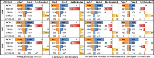
(1) All global GHG emissions continue to grow, with CO₂ increasing the most, Fgas growing the fastest, and the overall growth rate of NCO₂ being slower than that of CO₂.

From 2004 to 2011, the total global emissions and per capita emissions of CO₂ increased by 19.94% and 10.47%, respectively; CO₂ emissions in 2011 increased by 5.02 billion tons compared with those in 2004 and had the largest emissions base and emissions increase. The total Fgas emissions and per capita emissions increased by 52.93% and 40.84%, respectively, and had the smallest emissions base but the fastest growth. The total growth rate of CH₄ and N₂O emissions was between 10% and 12%, and the per capita emissions growth rate was between 2% and 3%, which was relatively slow. The overall growth rate of NCO₂ emissions was 13.28%, which was slower than that of CO₂ (Figure 1). China, the US, India, Russia, Japan, and Germany had the largest total GHG emissions in the world. The total GHG production and consumption emissions of these six countries accounted for about 55% of the global total. Kuwait (60.05 tCO₂e/person) and Luxembourg (33.36 tCO₂e/person) were the countries with the highest per capita GHG production and consumption emissions; “East Timor + Myanmar” (0.18 and 0.34 tCO₂e/person) was the region with the lowest per capita GHG production and consumption emissions. Countries with the highest and lowest per capita GHG production and consumption emissions were all BRI countries. In general, developing and least developed countries represented by China, India, Russia, and Pakistan are generally in the stage of rapid economic and social development and currently have the largest and fastest growth in GHG production and consumption emissions. For the group of developed countries, the internal situation differs. The EU countries are the pioneers in leading the simultaneous decline of production and consumption emissions. The US, Canada, Japan, Australia, and other umbrella group countries present different variations in their production and consumption emissions – some increased, while some others decreased.

(2) Among the four major groups, BRI-88’s global share of GHGs is relatively stable, and consumption emissions are growing faster than production emissions. China’s GHG emissions have the largest increase and the fastest growth rate. NBRI-34 has the largest total emissions but shows negative growth in CO₂ emission.

From 2004 to 2011, the production and consumption emissions of all gases of BRI-88 had been increasing slowly and simultaneously. Consumption emissions grew slightly faster than production emissions, but the global share of GHG production and consumption emissions was relatively stable at about 30%. China, the main driver of global GHG emissions growth, also saw production and consumption emissions of all gases grow rapidly. The growth rate of consumption emissions was significantly faster than that of the production emissions. Its global share of GHG production and consumption emissions both increased by more than 7 percentage points. The GHG production and consumption emissions of NBRI-34 account for more than 40% and 45%, respectively, of the total global emissions, making NBRI-34 the largest emitting group. NBRI-34’s global production and consumption of Fgas accounted for about 60% of the global total, exceeding the sum of other groups. However, its CO₂ production and consumption emissions experienced negative growth during the 2007–2011 period, decreasing its global share of GHG production and consumption emissions by 6.1 and 8.2 percentage points, respectively. Consumption emissions fell faster than production emissions.

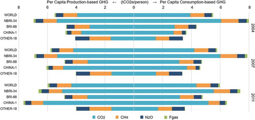
Figure 2. Composition in per capita production-based and consumption-based GHG emissions in 2004, 2007, and 2011

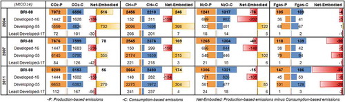
(3) NBRI-34 is the largest net importer group of GHGs; China is the largest net exporter of GHGs; and BRI-88 is a net exporter of CO₂ and CH₄, and a net importer of N₂O and Fgas. A significant difference exists in the emission intensity of different gases among the groups.

From 2004 to 2011, NBRI-34 was the largest net importer of GHGs, with consumption emissions of all gases greater than production emissions, but its net import emissions of CO₂, CH₄, and N₂O continued to decline. Moreover, it transformed into a net export group from a net import group of Fgas during 2007–2011, replacing China as the world’s largest net exporter of Fgas. In 2011, NBRI-34’s GHG net import emissions dropped to 1.49 billion tCO₂e. The US, Japan, UK, and Germany were the largest net importers of GHGs in NBRI-34. China was the largest net GHG exporter with all gases’ production emissions larger than consumption emissions. China’s CO₂ and Fgas net export emissions initially increased and then decreased, whereas CH₄ and N₂O continued to decline. China’s net GHG export emissions in 2011 were 1.50 billion tCO₂e. BRI-88 was a GHG net exporter whose GHG production emissions exceeded GHG consumption emissions. BRI-88 net export emissions of CO₂ and CH₄ continued to decline, and its net import emissions of N₂O and Fgas continued to increase. In 2011, BRI-88’s net GHG export emissions dropped to 56 million tCO₂e. Russia, South Africa, Kazakhstan, Kuwait, and South Korea were characteristic GHG net exporters of BRI-88 (Figure 1). In general, China and BRI-88’s net GHG export emissions and NBRI-34’s net GHG import emissions decreased simultaneously. The GHG transfer emissions among groups shrank. In terms of per capita emissions, NBRI-34’s per capita consumption emissions of CO₂ (7.40 t/person), CH₄ (1.13 tCO₂e/person), and Fgas (0.20 tCO₂e/person) have always been the highest levels in the world. China’s per capita production and consumption emissions of CH₄ (0.83 and 0.78 tCO₂e/person) and N₂O (0.42 and 0.38 tCO₂e/person) were historically the lowest in the world. CO₂ (6.46 t/person) and Fgas (0.12 tCO₂e/person) consumption per capita emissions have been higher than the global average. China’s per capita CO₂ production emissions exceeded those of NBRI-34 from 2007 to 2011 and reached 7.67 t/person, the highest level in the world (i.e., 1.45 times the global average). The per capita production and consumption emissions of CO₂ (3.22 and 3.20 t/person) and Fgas (0.06 and 0.07 tCO₂e/person) of BRI-88 are significantly lower than the global average, and CH₄ (1.05 and 0.98 tCO₂e/person) and N₂O (0.51 and 0.53 tCO₂e/person) per capita production and consumption emissions are roughly equivalent to the global average (Figure 2).

(4) The sectoral distribution varies among gases, country groups, as well as for production-based and consumption-based emissions. CO₂ and Fgas emissions are more concentrated on the production side, but more dispersed across sectors on the consumption side. The sectoral distribution of CH₄ and N₂O is relatively dispersed across sectors on both the production and consumption sides.

Figure 3. Sectoral contribution of production-based and consumption-based emissions of specific GHGs, 2011

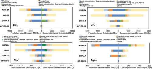
From the production emission perspective, in 2011, electricity, transport, nonmetallic minerals, and ferrous metals contributed up to 63.25% of global CO₂ production emissions, of which a quarter came from BRI-88. In terms of BRI-88, the electricity sector contributed the most to production-based CO₂ emissions (3530.80 million tCO₂; 43.01%), followed by the transport sector (993.93 million tCO₂; 12.11%). From the consumption perspective, construction, electricity, government services (public administration, defense, education, health), and other machinery and equipment contributed 43.10% of global CO₂ consumption-based emissions, of which 24% came from BRI-88. The electricity (1173.30 million tCO₂; 14.39%) and the construction (960.61 million tCO₂; 11.78%) sectors are the two largest contributing sectors from the consumption-based perspective.

For CH₄ emissions, the sectors that contribute the most to global CH4 production emissions are government services (public administration, defense, education, health), and animal products, with a total contribution rate of 54.62%, of which 33.50% comes from BRI-88. The largest contribution sectors to global CH₄ consumption emissions are government services, construction, and animal and meat products, with a total contribution rate of 46.06%, of which 35.69% comes from BRI-88. As for BRI-88, government services (public administration, defense, education, health) is the largest contributor to CH₄ production and consumption emissions of BRI-88, with contribution shares of 22.00% (586.19 million tCO₂e) and 26.62% (659.41 million tCO₂e), respectively. Animal products, construction, and meat products are the other main sources of BRI-88’s CH₄ consumption emissions. For NCO₂ emissions, the sectors that contribute the most to global N2O production emissions are animal products, vegetables and fruits, and raw milk, with a total contribution rate of 58.92%, of which 36.57% comes from BRI-88. Animal products and vegetables and fruits contributed 37.38% (484.93 million tCO₂e) of the production-based N₂O emissions in BRI-88. The sectors that contribute the most to global N2O consumption emissions are animal products, government services (public administration, defense, education, health), vegetables, food, and meat products, with a total contribution rate of 42.89%, of which 37.78% comes from BRI-88. Animal products and vegetables and fruits contributed 22.16% (296.77 million tCO₂e) of the consumption-based N₂O emissions in BRI-88. For Fgas, all global production-based Fgas emissions come from four sectors, namely, electronic equipment, chemical rubber products, electricity, and non-ferrous metals. Among the different groups, BRI-88 contributed 16.95% (146.74 million tCO₂e). For the consumption-based Fgas emissions, electronic equipment, other government services, construction, other machinery and equipment, and chemical rubber products contributed 69.30% of Fgas emissions globally, of which 21.53% (185.54 million tCO₂e) came from BRI-88 (Figure 3). Electronic equipment contributed the most to BRI-88’s production-based Fgas emissions (105.14 million tCO₂e, 21.61%) and consumption-based Fgas emissions (70.51 million tCO₂e, 23.93%). Construction, non-ferrous metals, government services, and chemical rubber products ranked as the second-tier main sources of BRI-88’s consumption-based Fgas emissions.

Production-based and consumption-based GHG emissions inside BRI-88

The population share of BRI-88 is basically stable, and the global share of GDP is slowly rising. In 2011, the population of BRI-88 accounted for 36.63% of the world’s population, comparable to that of the NBRI-34 group, but its GDP accounted for only 22.92%, which was only one-third of the NBRI-34 group’s share (Figure 4). BRI-88’s GHG production and consumption emissions have continued to increase, reaching 12.32 and 12.17 billion tCO₂e in 2011, respectively. CO₂ accounted for about two-thirds and NCO₂ accounted for about one-third.

Figure 4. Comparison of population, GDP, and GHG emissions by groups with different levels of development in 2011

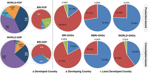
Figure 5. Per capita GHG emissions of BRI-88 and groups with different development levels

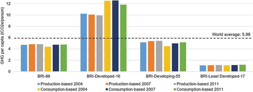
(1) The 55 developing countries are the main emitters with BRI-88, with huge potential for growth. The per capita emissions intensity of BRI countries with different levels of development significantly varies.

From the perspective of total emissions, the emissions from production and consumption in 55 developing countries in the BRI-88 region accounted for 80.94% and 77.76% of all BRI-88 emissions in 2011, respectively. In terms of GHG emissions per capita, the GHG production and consumption emissions per capita of BRI-88 in 2011 were 4.83 and 4.78 tCO₂e/person, respectively, which were both lower than the global average (5.98 tCO₂e/person). Further comparison of GHG per capita consumption emissions of countries with different levels of development within the BRI domain reveals that the developed countries (11.84 tCO₂e/person) rank the highest, which is about twice the global average, whereas developing countries (5.16 tCO₂e/person) and least developed countries (1.18 tCO₂e/person) are lower than the global average. From 2004 to 2011, the per capita GHG production and consumption emissions of 55 developing countries and 17 least developed countries within the BRI-88 region continued to increase (Figure 5).

Figure 6. Per capita GHG consumption emissions of countries within the BRI-88 and NBRI-34 groups – GDP per capita distribution, 2011

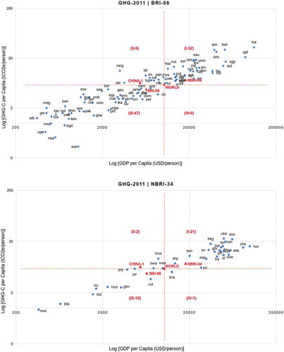
(2) The total amount of GHG emissions of member countries within the BRI-88 domain varies greatly. The imbalance in per capita emissions intensity is more significant than that of NBRI-34. Most BRI countries remain in a low-income development stage with low emissions.

In terms of total emissions, the BRI country with the most amount of GHG production and consumption emissions in 2011 was Russia (2.26 and 1.94 billion tCO₂e), whereas the countries with the lowest GHG production and consumption emissions were Malta (3 Million tCO₂e) and Rwanda (5 Million tCO₂e), respectively. The gap between the highest and lowest production and consumption emissions was 723 times and 430 times, respectively. The total GHG production and consumption emissions of Russia, Indonesia, South Korea, Iran, Saudi Arabia, Italy, and other top 10 highest emissions BRI countries account for 55.42% and 54.74% of the total BRI-88 emissions, respectively. From the perspective of per capita emissions, the countries with the highest per capita GHG production and consumption emissions in the BRI-88 domain in 2011 were Kuwait (60.05 tCO₂e/person) and Luxembourg (33.36 tCO₂e/person). The lowest were in “East Timor + Myanmar” (0.18 and 0.34 tCO₂e/person, respectively) in Southeast Asia. The differences between the highest and lowest countries in production and consumption emissions were 335 and 98 times, respectively, i.e., significantly larger than the respective 22 and 24 times of NBRI-34. Moreover, the wealth gap among countries within the BRI-88 region is also more significant than that of NBRI-34. The difference between the country with the highest per capita GDP (Luxembourg) and the lowest GDP (Ethiopia) is 319 times (272 times in NBRI). As shown in Figure 6, per capita GHG consumption emissions have a strong positive correlation with per capita GDP. Four quadrants are made with world per capita GDP and world per capita GHG emission intensity as the origin; 32 BRI countries such as Luxembourg, Russia, South Korea, and Singapore fall into quadrant I (high-income, high-emissions), which includes all developed countries and 16 developing countries within BRI-88, most of which are located in the EU+ and the Middle East. Ten developing countries including Mongolia, South Africa, Malaysia, and Belarus fall into quadrant II, which is characterized by low income and high emissions. Forty-seven BRI countries such as Indonesia, Vietnam, the Philippines, and Cambodia fall into quadrant III, which is characterized by low income and low emissions, including all less developed countries and 30 developing countries within BRI-88. Quadrants II and III show the largest differences in the distribution of BRI-88 and NBRI-34. The 57 BRI countries that fall into these two quadrants may be important sources of emissions growth for basic demand satisfaction and development.

Figure 7. Composition of production and consumption emissions and changes in the net embodied emissions of BRI-88 and its groups with different levels of development in 2004, 2007, and 2011

(3) The developed countries within BRI-88 are the main net importers of GHGs, and the developing countries are the main net exporters. The internal “offset” decreases the significance of the overall transfer emissions of BRI-88, whereas the import and export emissions of different countries in the region significantly varies.

On the whole, for CO₂ and CH₄, BRI-88 is basically aligned with the finding that developing country groups are net exporters and developed country groups are net importers (Zhang et al. 2018). However, for N₂O and Fgas, the 55 developing countries in BRI-88 have gradually transformed from net exporters to net importers (Figure 7). From 2004 to 2011, the proportion of production-based and consumption-based GHG emissions within BRI-88 continued to increase from 77.74% (7.58 billion tCO₂e) in 2004 to 80.42% (8.92 billion tCO₂e) in 2011. By contrast, GHG emissions for net exports gradually decreased to less than 20%. However, from the perspective of BRI countries, 34 GHG net exporters and 53 GHG net importers were in BRI-88 in 2011. Net exports and net import emissions totaled 1.01 billion and 866 million tCO₂e, respectively. Among them, Russia (0.32 billion tCO₂e) is the largest net GHG exporter, Italy (0.20 billion tCO₂e) is the largest net GHG importer, and Kuwait is the country with both the highest proportion of GHG net export emissions in production emissions (50.27%) and net GHG import emissions as a proportion of consumption emissions (101.09%).

Embodied emissions flows in global imports and exports

The embodied GHG emissions in global trade increased from 5.51 billion tCO₂e in 2004 to 6.60 billion tCO₂e in 2011; however, the global share was basically stable, ranging between 15% and 16%. The ratio of CO₂ to NCO₂ in the embodied emissions of global trade is about 7:3.

Figure 8. Global GHG import and export emissions flows in 2004, 2007, and 2011

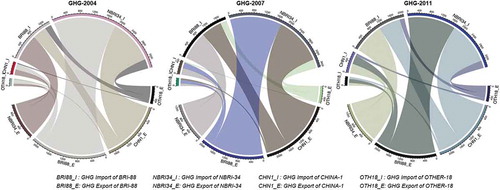
(1) BRI-88’s export emissions initially decreased and then increased, but import emissions continued to grow rapidly. Export emissions flowed mostly to NBRI-34, and import emissions also primarily originated from NBRI-34, followed by China.

In 2004, BRI-88 (2.17 billion tCO₂e) was the largest GHG exporter among the four groups. Later on, its GHG export emissions initially decreased and then increased and returned in 2011 (2.17 billion tCO₂e) to a comparable level as in 2004. About 20% of BRI-88’s GHG production emissions are used for net exports, and these emissions flowed mostly to NBRI-34, followed by China. From 2004 to 2011, the proportion of emissions that flowed to NBRI-34 among the total BRI-88 export emissions decreased from 86.86% (1.89 billion tCO₂e) in 2004 to 78.99% (1.72 billion tCO₂e) in 2011. However, NBRI-34 has always been the main export destination, though the share of emissions that flowed to China has continued to increase from 7.97% (0.17 billion tCO₂e) to 14.53% (0.31 billion tCO₂e). BRI-88 has always been the second largest importer in the world after NBRI-34, and its import emissions continued to grow, reaching 1.42, 1.86, and 2.03 billion tCO₂e in 2004, 2007, and 2011, respectively. These values account for 18–19% of its GHG consumption emissions. The import emissions of BRI-88 primarily originated from NBRI-34, followed by China. Emissions imported from NBRI-34 increased during 2004–2011 (from 803 million to 1.07 billion tCO₂e) but the proportion decreased (from 56.68% to 52.89%). Meanwhile, emissions imported from China, and their proportions, continued to increase from 29.65% (0.42 billion tCO₂e) to 38.29% (0.78 billion tCO₂e).

Figure 9. Global import and export emissions flow of four types of GHGs in 2011

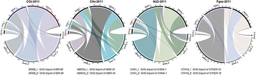
(2) The embodied import and export emissions for the four GHG gases within the BRI-88 group rank first or second in the world.

In 2011, 6.60 billion tCO₂e of GHG emissions were embodied in global trade. Of this amount, CO₂ accounts for 70.24% (4.63 billion tCO₂e); China is the largest exporter, followed by BRI-88, and NBRI-34 is the largest importer, followed by BRI-88. CH₄ accounts for 18.44% (1.22 billion tCO₂e); BRI-88 is the largest exporter; NBRI-34 is the largest importer, followed by BRI-88. N₂O accounts for 7.87% (0.52 billion tCO₂e); NBRI-34 is the largest exporter, followed by BRI-88; NBRI-34 is the largest importer, followed by BRI-88. Fgas accounts for 3.45% (0.23 billion tCO₂e); NBRI-34 is the largest exporter, followed by China; BRI-88 is the largest importer, followed by NBRI-34 (Figure 9).

(3) Import and export emissions based on international trade between BRI-88 and China began to increase from 2004 to 2011. BRI-88’s net imports of GHG emissions from China are primarily CO₂.

From the perspective of GHGs as a whole, the emissions BRI-88 imported from China increased by 66.46% and 11.16% in the two stages of 2004–2007 and 2007–2011, respectively; the average annual growth rate during the period of 2004–2011 was 9.19%. In 2004–2007 and 2007–2011, the emissions BRI-88 exported to China increased by 13.52% and 60.80%, respectively. The average annual growth rate during 2004–2011 was 8.98%. As early as 2004–2011 before the BRI was proposed, the interaction and the import and export emissions between BRI-88 and China increased over time (Figure 8). In 2011, 14.53% (0.32 billion tCO₂e) of BRI-88’s GHG export emissions flowed to China, and 38.29% (0.78 billion tCO₂e) of import emissions came from China. Therefore, BRI-88 is the main importer of GHGs between the two. In 2004, 2007, and 2011, the GHG emissions of BRI-88 net imports from China were 247, 503, and 461 million tCO₂e. Of the 461 million tCO₂e of net import emissions in 2011, CO₂, CH₄, N₂O, and Fgas accounted for 426, 4, 19, and 12 million tCO₂e, and CO₂ accounted for 92.41% (Figure 9).

Figure 10. Changes in embodied emissions of imports and exports between China and BRI-88, as well as countries and regions within the domain, in 2004, 2007, and 2011

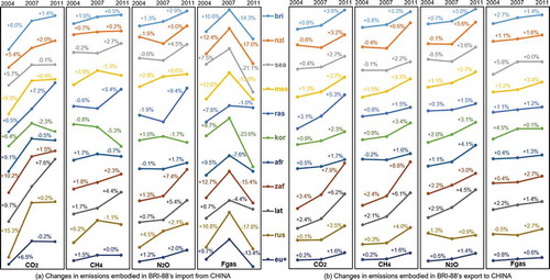
The overall BRI-88 GHG import and export emissions to and from China have continued to increase, with CO₂ growing faster than NCO₂. However, the growth rate of import and export emissions accelerated or slowed down in different countries and regions within the domain, presenting different situations. BRI-88 as a whole and its 10 countries and regions imported increasing amounts of CO₂, CH₄, and N₂O emissions from China, and the growth rate in the 2004–2007 period was faster than that of the 2007–2011 period. Meanwhile, the import emissions of Fgas in these two stages experienced a rapid rise followed by a rapid decline, with China’s Fgas export to BRI-88 partially shifting to NBRI-34 in the latter stage. From 2004 to 2011, in terms of BRI-88’s import emissions from China, gases with the largest average annual growth rate decreased in the order CO₂ (10.05%) > N₂O (8.39%) > Fgas (5.44%) > CH₄ (4.38%) (Figure 10-a). In 2011, the embodied emissions of CO₂, CH₄, N₂O, and Fgas imported from China by BRI-88 were 666, 73, 38, and 20 million tCO₂e. BRI-88 as a whole and its 10 countries and regions also continued to increase their export of the four GHGs to China, and the growth rate during 2007–2011 was significantly higher than that during 2004–2007. From 2004 to 2011, in terms of BRI-88’s export emissions to China, gases with the biggest average annual growth rate were, in decreasing order, CO₂ (9.51%) > N₂O (8.76%) > Fgas (8.01%) > CH₄ (7.57%) (Figure 10(b)). In 2011, the embodied emissions of CO₂, CH₄, N₂O, and Fgas exported to China by BRI-88 were 220, 69, 19, and 8 million tCO₂e. If BRI-88 were divided into 10 countries and regions based on geographical location (Appendix A), further analysis shows the following. Southeast Asia, EU+, and Middle East regions within the BRI-88 region would have the largest import emissions from China; Latin America and Russia would have the fastest increase in import emissions; New Zealand, South Korea, and the EU+ would have the slowest growth in import emissions (Figure 10(a)); Asian countries would have the most export emissions to China; South Africa and Latin America would have the fastest growth in export emissions; and Russia and the EU+ would have the slowest growth in export emissions (Figure 10(b)).

Discussion and conclusion

BRI is not only an important framework affecting the global economy, trade, and emission patterns broadly and profoundly, but BRI countries are also indispensable stakeholders that need to be included and consolidated to address global climate change. In this study, we estimated the total production-based, consumption-based, and embodied emissions of BRI-88 and their respective changes over time by using an MRIO model.

Our results show that both the production-based and consumption-based GHG emissions of BRI-88 increased during 2004–2011, with a growth rate slower than China but faster than NBRI-34. However, the per capita GHG production and consumption emissions of BRI-88 are still lower than the global average, a fact owing to the significant differences among country groups in BRI with different development levels. The per capita production and consumption emissions levels of the 55 developing countries in BRI-88 are still 20% lower than the global average, while the per capita consumption emissions levels of the 17 least developed countries are less than one-fifth of the global average – they are still in the low-income and low-emissions development stage, with massive growth potential. BRI-88 is a net exporter of CO₂ and CH₄ and a net importer of N₂O and Fgas. BRI-88’s GHG export emissions account for 16% of its production-based GHG emissions, of which about 80% and 15% flow to NBRI-34 and China, respectively; while about 57% and 38% of GHG import emissions came from NBRI-34 and China, respectively. From 2004 to 2011, trade-related GHG emissions between BRI-88 and China continued to increase.

Prior literature has identified a number of policy recommendations for managing emissions related to the BRI, such as identifying key environmental issues (Ascensão et al. 2018; Hughes et al. 2020) and improving green investment standards (Ma and Zadek 2019). Our research puts forward several policy recommendations specifically related to emissions accounting and embodied emissions in trade:

1) GHG emissions embodied in trade and their cross-border flows cannot be ignored – especially for BRI as an international cooperation platform. To encourage the scale-up of emissions mitigation efforts without sacrificing the strong economic growth potential of BRI as well as keeping climate risks under control, it is of great importance to refine the emissions accounting and responsibility-sharing system, which can objectively reflect the emissions responsibilities, decrease international trade disputes, and increase the participation of BRI countries in addressing climate change.

2) There is no one-size-fits-all solution for BRI countries with different development stages and emissions levels. However, for countries seeking low-carbon and sustainable development, they could take action in the following five aspects. Firstly, these countries can rationally plan and carefully select infrastructure construction projects and large-scale investments in order to avoid a high-emissions lock-in effect. Secondly, they can actively introduce and deploy green and low-emissions technologies and continuously improve technological efficiency by accelerating technological innovation. Thirdly, they can optimize the energy structure by developing renewable energy at large scale instead of fossil fuels. Fourthly, they can optimize the industrial structure by assessing the country’s context and comparative advantages. Last but not least, they can implement energy efficiency improvement and emissions mitigation strategies in the construction and transport sectors to promote a green and low-carbon lifestyle.

3) As BRI’s initiator as well as one of the most active participants, China plays a unique and important role. As the first step, China should lead the collaboration with multiple parties to build a green, low-emissions, and sustainable system of rules under the BRI framework in the areas of policies, projects (infrastructure), trade and trade agreements, finance, culture, and other relevant areas, in order to promote BRI countries’ green development and global climate governance. Then, by working closely with NBRI countries to make the most of this unparalleled platform to strengthen green and low-carbon cooperation, China can help accelerate the dissemination and deployment of effective and feasible green and low-carbon technologies, knowledge, finance, and policies in the BRI domain, and assist BRI countries in capacity building.

Additional information

Funding

This work was supported by the National Key Research and Development Program of China [2018YFA0606503]; the National Natural Science Foundation of China [71590243,71673162].

Notes

¹ Source: https://www.yidaiyilu.gov.cn/gbjg/gbgk/77073.htm.

² Source: https://www.gtap.agecon.purdue.edu.

³ Source: https://www.exiobase.eu.

⁴ Source: http://www.wiod.org/home.

⁵ Source: https://www.worldmrio.com.

⁶ Includes the study of China’s national greenhouse gas list (2005, 2008, and 2012), the second national information notification of the People’s Republic of China on climate change (2005) and the first biennial update of the People’s Republic of China on climate change (2012).

⁷ BRI country list obtained from the BRI official website at https://www.yidaiyilu.gov.cn/gbjg/gbgk/77073.htm.

Appendix A

Regional division of 140 countries and regions in the GTAP 9 database

Table

No.	Code 1	Description	World- 4 Group	BRI-10 Areas	Code 2
1	aus	Australia	NBRI-34	–	–
2	nzl	New Zealand	BRI-88	New Zealand	nzl
3	xoc	Rest of Oceania	OTHER-18	–	–
4	chn	China	CHINA-1	–	–
5	hkg	Hong Kong, Special Administrative Region of China	NBRI-34	–	–
6	jpn	Japan	NBRI-34	–	–
7	kor	Korea, Republic of	BRI-88	Korea	kor
8	mng	Mongolia	BRI-88	Rest of Asia	ras
9	twn	Taiwan	NBRI-34	–	–
10	xea	Rest of East Asia	OTHER-18	–	–
11	brn	Brunei Darussalam	BRI-88	Southeast Asia	sea
12	khm	Cambodia	BRI-88	Southeast Asia	sea
13	idn	Indonesia	BRI-88	Southeast Asia	sea
14	lao	Lao PDR	BRI-88	Southeast Asia	sea
15	mys	Malaysia	BRI-88	Southeast Asia	sea
16	phl	Philippines	BRI-88	Southeast Asia	sea
17	sgp	Singapore	BRI-88	Southeast Asia	sea
18	tha	Thailand	BRI-88	Southeast Asia	sea
19	vnm	Viet Nam	BRI-88	Southeast Asia	sea
20	xse*	Rest of Southeast Asia (Myanmar + Timor-Leste)	BRI-88	Southeast Asia	sea
21	bgd	Bangladesh	BRI-88	Rest of Asia	ras
22	ind	India	NBRI-34	–	–
23	npl	Nepal	BRI-88	Rest of Asia	ras
24	pak	Pakistan	BRI-88	Rest of Asia	ras
25	lka	Sri Lanka	BRI-88	Rest of Asia	ras
26	xsa	Rest of South Asia	OTHER-18	–	–
27	can	Canada	NBRI-34	–	–
28	usa	United States of America	NBRI-34	–	–
29	mex	Mexico	NBRI-34	–	–
30	xna	Rest of North America	OTHER-18	–	–
31	arg	Argentina	NBRI-34	–	–
32	bol	Bolivia	BRI-88	Latin America	lat
33	bra	Brazil	NBRI-34	–	–
34	chl	Chile	BRI-88	Latin America	lat
35	col	Colombia	NBRI-34	–	–
36	ecu	Ecuador	BRI-88	Latin America	lat
37	pry	Paraguay	NBRI-34	–	–
38	per	Peru	BRI-88	Latin America	lat
39	ury	Uruguay	BRI-88	Latin America	lat
40	ven	Venezuela (Bolivarian Republic of)	BRI-88	Latin America	lat
41	xsm	Rest of South America	OTHER-18	–	–
42	cri	Costa Rica	BRI-88	Latin America	lat
43	gtm	Guatemala	NBRI-34	–	–
44	hnd	Honduras	NBRI-34	–	–
45	nic	Nicaragua	NBRI-34	–	–
46	pan	Panama	BRI-88	Latin America	lat
47	slv	El Salvador	BRI-88	Latin America	lat
48	xca	Rest of Central America	OTHER-18	–	–
49	dom	Dominican Republic P	BRI-88	Latin America	lat
50	jam	Jamaica	BRI-88	Latin America	lat
51	pri	Puerto Rico	NBRI-34	–	–
52	tto	Trinidad and Tobago P	BRI-88	Latin America	lat
53	xcb	Rest of Caribbean	OTHER-18	–	–
54	aut	Austria	BRI-88	European Union+	eu+
55	bel	Belgium	NBRI-34	–	–
56	cyp	Cyprus	BRI-88	European Union+	eu+
57	cze	Czech Republic	BRI-88	European Union+	eu+
58	dnk	Denmark	NBRI-34	–	–
59	est	Estonia	BRI-88	European Union+	eu+
60	fin	Finland	NBRI-34	–	–
61	fra	France	NBRI-34	–	–
62	deu	Germany	NBRI-34	–	–
63	grc	Greece	BRI-88	European Union+	eu+
64	hun	Hungary	BRI-88	European Union+	eu+
65	irl	Ireland	NBRI-34	–	–
66	ita	Italy	BRI-88	European Union+	eu+
67	lva	Latvia	BRI-88	European Union+	eu+
68	ltu	Lithuania	BRI-88	European Union+	eu+
69	lux	Luxembourg	BRI-88	European Union+	eu+
70	mlt	Malta	BRI-88	European Union+	eu+
71	nld	Netherlands	NBRI-34	–	–
72	pol	Poland	BRI-88	European Union+	eu+
73	prt	Portugal	BRI-88	European Union+	eu+
74	svk	Slovakia	BRI-88	European Union+	eu+
75	svn	Slovenia	BRI-88	European Union+	eu+
76	esp	Spain	NBRI-34	–	–
77	swe	Sweden	NBRI-34	–	–
78	gbr	United Kingdom	NBRI-34	–	–
79	che	Switzerland	NBRI-34	–	–
80	nor	Norway	NBRI-34	–	–
81	xef	Rest of European Free Trade Association	OTHER-18	–	–
82	alb	Albania	BRI-88	European Union+	eu+
83	bgr	Bulgaria	BRI-88	European Union+	eu+
84	blr	Belarus	BRI-88	European Union+	eu+
85	hrv	Croatia	BRI-88	European Union+	eu+
86	rou	Romania	BRI-88	European Union+	eu+
87	rus	Russian Federation	BRI-88	Russian Federation	rus
88	ukr	Ukraine	BRI-88
89	xee	Rest of Eastern Europe	BRI-88
90	xer	Rest of Europe	OTHER-18	–	–
91	kaz	Kazakhstan	BRI-88	Rest of Asia	ras
92	kgz	Kyrgyztan	BRI-88	Rest of Asia	ras
93	xsu	Rest of Former Soviet Union	OTHER-18	–	–
94	arm	Armenia	BRI-88	Rest of Asia	ras
95	aze	Azerbaijan	BRI-88	Rest of Asia	ras
96	geo	Georgia	BRI-88	Rest of Asia	ras
97	bhr	Bahrain	BRI-88	Middle East	mea
98	irn	Iran, Islamic Republic of	BRI-88	Middle East	mea
99	isr	Israel	NBRI-34	–	–
100	jor	Jordan	NBRI-34	–	–
101	kwt	Kuwait	BRI-88	Middle East	mea
102	omn	Oman	BRI-88	Middle East	mea
103	qat	Qatar	BRI-88	Middle East	mea
104	sau	Saudi Arabia	BRI-88	Middle East	mea
105	tur	Turkey	BRI-88	Middle East	mea
106	are	United Arab Emirates	BRI-88	Middle East	mea
107	xws	Rest of Western Asia	OTHER-18	–	–
108	egy	Egypt	BRI-88	Africa	afi
109	mar	Morocco	BRI-88	Africa	afi
110	tun	Tunisia	BRI-88	Africa	afi
111	xnf	Rest of North Africa	OTHER-18	–	–
112	ben	Benin	BRI-88	Africa	afi
113	bfa	Burkina Faso	NBRI-34	–	–
114	cmr	Cameroon	BRI-88	Africa	afi
115	civ	Côte d’Ivoire	BRI-88	Africa	afi
116	gha	Ghana	BRI-88	Africa	afi
117	gin	Guinea	BRI-88	Africa	afi
118	nga	Nigeria	BRI-88	Africa	afi
119	sen	Senegal	BRI-88	Africa	afi
120	tgo	Togo	BRI-88	Africa	afi
121	xwf	Rest of Western Africa	OTHER-18	–	–
122	xcf	Rest of Central Africa	OTHER-18	–	–
123	xac	South Central Africa	OTHER-18	–	–
124	eth	Ethiopia	BRI-88	Africa	afi
125	ken	Kenya	BRI-88	Africa	afi
126	mdg	Madagascar	BRI-88	Africa	afi
127	mwi	Malawi	NBRI-34	–	–
128	mus	Mauritius	NBRI-34	–	–
129	moz	Mozambique	BRI-88	Africa	afi
130	rwa	Rwanda	BRI-88	Africa	afi
131	tza	Tanzania, United Republic of	BRI-88	Africa	afi
132	uga	Uganda	BRI-88	Africa	afi
133	zmb	Zambia	BRI-88	Africa	afi
134	zwe	Zimbabwe	BRI-88	Africa	afi
135	xec	Rest of Eastern Africa	OTHER-18	–	–
136	bwa	Botswana	NBRI-34	–	–
137	nam	Namibia	BRI-88	Africa	afi
138	zaf	South Africa	BRI-88	South Africa	zaf
139	xsc	Rest of South African Customs Union	OTHER-18	–	–
140	xtw	Rest of the World	OTHER-18	–	–

Appendix B

GTAP 9 Database Sectors

Table

No.	Code	Description	No.	Code	Description
1	PDR	Paddy rice	30	LUM	Wood products
2	WHT	Wheat	31	PPP	Paper products, publishing
3	GRO	Cereal grains nec	32	P_C	Petroleum, coal products
4	V_F	Vegetables, fruit, nuts	33	CRP	Chemical, rubber, plastic products
5	OSD	Oil seeds	34	NMM	Mineral products nec
6	C_B	Sugar cane, sugar beet	35	I_S	Ferrous metals
7	PFB	Plant-based fibers	36	NFM	Metals nec
8	OCR	Crops nec	37	FMP	Metal products
9	CTL	Bovine cattle, sheep and goats, horses	38	MVH	Motor vehicles and parts
10	OAP	Animal products nec	39	OTN	Transport equipment nec
11	RMK	Raw milk	40	ELE	Electronic equipment
12	WOL	Wool, silk-worm cocoons	41	OME	Machinery and equipment nec
13	FRS	Forestry	42	OMF	Manufactures nec
14	FSH	Fishing	43	ELY	Electricity
15	COA	Coal	44	GDT	Gas manufacture, distribution
16	OIL	Oil	45	WTR	Water
17	GAS	Gas	46	CNS	Construction
18	OMN	Minerals nec	47	TRD	Trade
19	CMT	Bovine meat products	48	OTP	Transport nec
20	OMT	Meat products nec	49	WTP	Water transport
21	VOL	Vegetable oils and fats	50	ATP	Air transport
22	MIL	Dairy products	51	CMN	Communication
23	PCR	Processed rice	52	OFI	Financial services nec
24	SGR	Sugar	53	ISR	Insurance
25	OFD	Food products nec	54	OBS	Business services nec
26	B_T	Beverages and tobacco products	55	ROS	Recreational and other services
27	TEX	Textiles	56	OSG	Public Administration, Defense, Education, Health
28	WAP	Wearing apparel	57	DWE	Dwellings
29	LEA	Leather products

Appendix C

Sector Mapping Rules of Non-CO₂ Greenhouse Gas Emissions

Table

Abbreviation	US EPA Data Base Sector/Source	IPCC	GTAP 9 Data Base Sector
ADNI	Adipic Acid and Nitric Acid Production	2B	Chemical, rubber, plastic products
ALUM	Primary Aluminum Production	2 C3	Metals nec
COAL	Coal Mining Activities	1B1	Coal
ELTD	Electric Power Systems	2F7a	Electricity
		2F7b
		2F7 c
HF22	HCFC-22 Production	2E	Chemical, rubber, plastic products
HUMS	Human Sewage-Domestic Wastewater/Landfilling of Solid Waste	6B	Public Administration, Defense, Education, Health
INCH	Other Industrial Processes Sources	2B	Chemical, rubber, plastic products
		2 C	Ferrous metals/Metals nec
		N/A	Mineral products nec/Manufactures nec/Paper products, publishing
INN2	Other Industrial Processes Sources	2B	Chemical, rubber, plastic products
INN2	Other Industrial Processes Sources	2C	Ferrous metals
		N/A	Manufactures nec/Paper products, publishing
LNDF	Landfilling of Solid Waste/Other Waste Sources	6A	Public Administration, Defense, Education, Health
MAGN	Magnesium Manufacturing	2C4	Metals nec
ODS	Use of Substitutes for Ozone Depleting Substances	2F1	Electronic equipment
		2F2	Chemical, rubber, plastic products
		2F3	Chemical, rubber, plastic products
		2F4	Chemical, rubber, plastic products
		N/A	Chemical, rubber, plastic products
OLGS	Natural Gas and Oil Systems	1B2	Gas manufacture, distribution/Transport nec/Petroleum, coal products/Oil/Gas
SEMI	Semiconductor Manufacturing/Flat Panel Display Manufacturing/Photovoltaic Manufacturing	2F7a	Electronic equipment
		2F7b
		2F7 c
SMCH	Stationary and Mobile Combustion/Other Energy Sources	1A(all)	Dwellings
SMN2	Stationary and Mobile Combustion/Other Energy Sources	1A(all)	Dwellings
WWTR	Wastewater	6B	Public Administration, Defense, Education, Health
BBCH	Biomass Combustion	4E	Bovine cattle, sheep and goats, horses
		4 F	Paddy rice/Wheat/Cereal grains nec/Vegetables, fruit, nuts/Oil seeds/Sugar cane, sugar beet/Plant-based fibers/Crops nec
BBN2	Biomass Combustion	4E	Bovine cattle, sheep and goats, horses
		4 F	Paddy rice/Wheat/Cereal grains nec/Vegetables, fruit, nuts/Oil seeds/Sugar cane, sugar beet/Plant-based fibers/Crops nec
EFRM	Enteric Fermentation	4A	Bovine cattle, sheep and goats, horses/Raw milk/Animal products nec
MNCH	Manure Management	4B	Bovine cattle, sheep and goats, horses/Raw milk/Animal products nec
MNN2	Manure Management	4B	Bovine cattle, sheep and goats, horses/Raw milk/Animal products nec
PRPD	Other Agriculture Sources	4D3	Bovine cattle, sheep and goats, horses/Raw milk/Animal products nec
RICE	Rice Cultivation/Other Agriculture Sources	4 C	Paddy rice
SOIL	Agricultural Soils	4D	Paddy rice/Wheat/Cereal grains nec/Vegetables, fruit, nuts/Oil seeds/Sugar cane, sugar beet/Plant-based fibers/Crops nec/Bovine cattle, sheep and goats, horses/Raw milk/Animal products nec

References

- Andrew, R. M., and G. P. Peters. 2013. “A Multi-Region Input–Output Table Based on the Global Trade Analysis Project Database (Gtap-mrio).” Economic Systems Research 25 (1): 99–20. doi:10.1080/09535314.2012.761953.
- Ascensão, F., L. Fahrig, A. P. Clevenger, R. T. Corlett, J. A. G. Jaeger, W. F. Laurance, and H. M. Pereira. 2018. “Environmental Challenges for the Belt and Road Initiative.” Nature Sustainability 1 (5): 206–209. doi:10.1038/s41893-018-0059-3.
- Breidenich, C., D. Magraw, A. Rowley, and J. Rubin. 1998. “Kyoto Protocol (KP) to the United Nations Framework Convention on Climate Change.” The American Journal of International Law 92: 315. doi:10.2307/2998044.
- Brunner, P. H., and H. Rechberger. 2004. Practical Handbook of Material Flow Analysis. Boca Raton: Lewis Publishers.
- Cai, X., X. Che, B. Zhu, J. Zhao, and R. Xie. 2018. “Will Developing Countries Become Pollution Havens for Developed Countries? an Empirical Investigation in the Belt and Road.” Journal of Cleaner Production 198: 624–632. doi:10.1016/j.jclepro.2018.06.291.
- Chen, G. Q., X. D. Wu, J. Guo, J. Meng, and C. Li. 2019. “Global Overview for Energy Use of the World Economy: Household-consumption-based Accounting Based on the World Input-output Database (WIOD).” Energy Economics 81: 835–847. doi:10.1016/j.eneco.2019.05.019.
- Chen, Y., S. Liu, H. Wu, X. Zhang, and Q. Zhou. 2020. “How Can Belt and Road Countries Contribute to Glocal Low-carbon Development?” Journal of Cleaner Production 256: 120717. doi:10.1016/j.jclepro.2020.120717.
- Davis, S. J., and K. Caldeira. 2010. “Consumption-based Accounting of CO2 Emissions.” Proceedings of the National Academy of Sciences 107 (12): 5687–5692. doi:10.1073/pnas.0906974107.
- Ding, T., Y. Ning, and Y. Zhang. 2018. “The Contribution of China’s Bilateral Trade to Global Carbon Emissions in the Context of Globalization.” Structural Change and Economic Dynamics 46: 78–88. doi:10.1016/j.strueco.2018.04.004.
- Fan, J.-L., Y.-B. Da, S.-L. Wan, M. Zhang, Z. Cao, Y. Wang, and X. Zhang. 2019. “Determinants of Carbon Emissions in ‘Belt and Road Initiative’ Countries: A Production Technology Perspective.” Applied Energy 239: 268–279. doi:10.1016/j.apenergy.2019.01.201.
- Han, M., Q. Yao, W. Liu, and M. Dunford. 2018. “Tracking Embodied Carbon Flows in the Belt and Road Regions.” Journal of Geographical Sciences 28 (9): 1263–1274. doi:10.1007/s11442-018-1524-7.
- Hertwich, E. G. 2005. “Life Cycle Approaches to Sustainable Consumption: A Critical Review.” Environmental Science & Technology 39: 4673–4684. doi:10.1021/es0497375.
- Hertwich, E. G., and G. P. Peters. 2009. “Carbon Footprint of Nations: A Global, Trade-Linked Analysis.” Environmental Science & Technology 43: 6414–6420. doi:10.1021/es803496a.
- Hu, J., R. Wood, A. Tukker, H. Boonman, and B. de Boer. 2019. “Global Transport Emissions in the Swedish Carbon Footprint.” Journal of Cleaner Production 226: 210–220. doi:10.1016/j.jclepro.2019.03.263.
- Huang, Y. 2019. “Environmental Risks and Opportunities for Countries along the Belt and Road: Location Choice of China’s Investment.” Journal of Cleaner Production 211: 14–26. doi:10.1016/j.jclepro.2018.11.093.
- Hubacek, K., and K. Feng. 2016. “Comparing Apples and Oranges: Some Confusion about Using and Interpreting Physical Trade Matrices versus Multi-regional Input–output Analysis.” Land Use Policy 50: 194–201. doi:10.1016/j.landusepol.2015.09.022.
- Hughes, A. C., A. M. Lechner, A. Chitov, A. Horstmann, A. Hinsley, A. Tritto, … D. W. Yu. 2020. “Horizon Scan of the Belt and Road Initiative.” Trends in Ecology & Evolution. doi:10.1016/j.tree.2020.02.005.
- Hung, C., S.-C. Hsu, and K.-L. Cheng. 2019. “Quantifying City-scale Carbon Emissions of the Construction Sector Based on Multi-regional Input-output Analysis.” Resources Conservation and Recycling 149: 75–85. doi:10.1016/j.resconrec.2019.05.013.
- IPCC. 2014. “Climate Change 2014: Mitigation of Climate Change.” Contribution of Working Group III to the Fifth Assessment Report of the Intergovernmental Panel on Climate Changee [Edenhofer, O., R. Pichs-Madruga, Y. Sokona, E. Farahani, S. Kadner, K. Seyboth, A. Adler, I. Baum, S. Brunner, P. Eickemeier, B. Kriemann, J. Savolainen, S. Schlömer, C. von Stechow, T. Zwickel and J.C. Minx (eds.)]. Cambridge University Press, Cambridge, United Kingdom and New York, NY, USA.
- Lenzen, M., K. Kanemoto, D. Moran, and A. Geschke. 2012. “Mapping the Structure of the World Economy.” Environmental Science & Technology 46 (15): 8374–8381. doi:10.1021/es300171x.
- Lenzen, M., -L.-L. Pade, and J. Munksgaard. 2010. “CO2Multipliers in Multi-region Input-Output Models.” Economic Systems Research 16 (4): 391–412. doi:10.1080/0953531042000304272.
- Li, Y. L., B. Chen, M. Y. Han, M. Dunford, W. Liu, and Z. Li. 2018. “Tracking Carbon Transfers Embodied in Chinese Municipalities’ Domestic and Foreign Trade.” Journal of Cleaner Production 192: 950–960. doi:10.1016/j.jclepro.2018.04.230.
- Liu, G., M. Wu, F. Jia, Q. Yue, and H. Wang. 2019. “Material Flow Analysis and Spatial Pattern Analysis of Petroleum Products Consumption and Petroleum-related CO2 Emissions in China during 1995–2017.” Journal of Cleaner Production 209: 40–52. doi:10.1016/j.jclepro.2018.10.245.
- Ma, J., and S. Zadek. 2019. “A Low-carbon Belt and Road.” https://www.project-syndicate.org/commentary/climate-change-belt-and-road-infrastructure-investment-by-ma-jun-and-simon-zadek-2019-03
- Mendelsohn, R. 2010. “World Development Report 2010: Development and Climate Change World Bank.” Journal of Economic Literature 48: 786–788. doi:10.2307/20778776.
- Meng, J., Z. Mi, D. Guan, J. Li, S. Tao, Y. Li, … S. J. Davis. 2018. “The Rise of South-South Trade and Its Effect on Global CO2 Emissions.” Nature Communications 9 (1): 1871. doi:10.1038/s41467-018-04337-y.
- Muhammad, S., X. Long, M. Salman, and L. Dauda. 2020. “Effect of Urbanization and International Trade on CO2 Emissions across 65 Belt and Road Initiative Countries.” Energy 196: 117102. doi:10.1016/j.energy.2020.117102.
- Ning, Z., Z. Liu, X. Zheng, and J. Xue. 2017. “Carbon Footprint of China’s Belt and Road.” Science 357: 1107. doi:10.1126/science.aao6621.
- Ohno, H., K. Matsubae, K. Nakajima, K. Nansai, Y. Fukushima, and T. Nagasaka. 2016. “Consumption-based Accounting of Steel Alloying Elements and Greenhouse Gas Emissions Associated with the Metal Use: The Case of Japan.” Journal of Economic Structures 5 (1): 1–17. doi:10.1186/s40008-016-0060-9.
- Pan, A., and L. Wei. 2015. “Embodied Carbon in Trade between China and Other BRICS Countries.” The Journal of Quantitative & Technical Economics 32: 54–70.
- Peters, G. P. 2007. “Opportunities and Challenges for Environmental MRIO Modelling: Illustrations with the GTAP Database.” In 16th International Input-Output Conference of the International Input-Output Association (IIOA), 1–26. Istanbul, Turkey.
- Peters, G. P. 2008. “From Production-based to Consumption-based National Emission Inventories.” Ecological Economics 65 (1): 13–23. doi:10.1016/j.ecolecon.2007.10.014.
- Peters, G. P., R. Andrew, and J. Lennox. 2011. “Constructing an Environmentally-Extended Multi-Regional Input–Output Table Using the Gtap Database.” Economic Systems Research 23 (2): 131–152. doi:10.1080/09535314.2011.563234.
- Peters, G. P., and E. G. Hertwich. 2006. “The Importance of Imports for Household Environmental Impacts.” Journal of Industrial Ecology 10: 89–109. doi:10.1162/jiec.2006.10.3.89.
- Peters, G. P., and E. G. Hertwich. 2008. “CO2 Embodied in International Trade with Implications for Global Climate Policy.” Environmental Science & Technology 42: 1401–1407. doi:10.1021/es072023k.
- Peters, G. P., J. Minx, C. Weber, and O. Edenhofer. 2011. “Growth in Emission Transfers via International Trade from 1990 to 2008.” Proceedings of the National Academy of Sciences 108: 8903–8908. doi:10.1073/pnas.1006388108.
- Rauf, A., X. Liu, W. Amin, I. Ozturk, O. U. Rehman, and M. Hafeez. 2018. “Testing EKC Hypothesis with Energy and Sustainable Development Challenges: A Fresh Evidence from Belt and Road Initiative Economies.” Environmental Science and Pollution Research 25 (32): 32066–32080. doi:10.1007/s11356-018-3052-5.
- Rauf, A., X. Liu, W. Amin, O. U. Rehman, J. Li, F. Ahmad, and F. Victor Bekun. 2020. “Does Sustainable Growth, Energy Consumption and Environment Challenges Matter for Belt and Road Initiative Feat? A Novel Empirical Investigation.” Journal of Cleaner Production 262: 121344. doi:10.1016/j.jclepro.2020.121344.
- Román, R., J. M. Cansino, and J. M. Rueda-Cantuche. 2016. “A Multi-regional Input-output Analysis of Ozone Precursor Emissions Embodied in Spanish International Trade.” Journal of Cleaner Production 137: 1382–1392. doi:10.1016/j.jclepro.2016.07.204.
- Sakai, M., and J. Barrett. 2016. “Border Carbon Adjustments: Addressing Emissions Embodied in Trade.” Energy Policy 92: 102–110. doi:10.1016/j.enpol.2016.01.038.
- Saud, S., S. Chen, A. Haseeb, and S. Sumayya. 2020. “The Role of Financial Development and Globalization in the Environment: Accounting Ecological Footprint Indicators for Selected One-belt-one-road Initiative Countries.” Journal of Cleaner Production 250: 119518. doi:10.1016/j.jclepro.2019.119518.
- Schaffartzik, A., D. Wiedenhofer, and N. Eisenmenger. 2015. “Raw Material Equivalents: The Challenges of Accounting for Sustainability in a Globalized World.” Sustainability 7 (5): 5345–5370. doi:10.3390/su7055345.
- Schmidt, S., C.-J. Södersten, K. Wiebe, M. Simas, V. Palm, and R. Wood. 2019. “Understanding GHG Emissions from Swedish Consumption - Current Challenges in Reaching the Generational Goal.” Journal of Cleaner Production 212: 428–437. doi:10.1016/j.jclepro.2018.11.060.
- Taherzadeh, O., and D. Caro. 2019. “Drivers of Water and Land Use Embodied in International Soybean Trade.” Journal of Cleaner Production 223: 83–93. doi:10.1016/j.jclepro.2019.03.068.
- Tamiotti, L., A. Olhoff, R. Teh, V. Kulacoglu, B. Simmons, and H. Abaza. 2009. Trade and Climate Change: A Report by the United Nations Environment Programme and the World Trade Organization. Genova: World Trade Organization ; United Nations Environment Programme.
- Teo, H. C., A. M. Lechner, G. W. Walton, F. K. S. Chan, A. Cheshmehzangi, M. Tan-Mullins, A. Campos-Arceiz, T. Sternberg, and A. Campos-Arceiz. 2019. “Environmental Impacts of Infrastructure Development under the Belt and Road Initiative.” Environments 6 (6): 72. doi:10.3390/environments6060072.
- Wang, Q., and Y. Zhou. 2019. “Uncovering Embodied CO2 Flows via North-North Trade - A Case Study of US-Germany Trade.” Science of the Total Environment 691: 943–959. doi:10.1016/j.scitotenv.2019.07.171.
- Wang, X., H. Zheng, Z. Wang, Y. Shan, J. Meng, X. Liang, D. Guan, and D. Guan. 2019. “Kazakhstan’s CO2 Emissions in the post-Kyoto Protocol Era: Production- and Consumption-based Analysis.” Journal of Environmental Management 249: 109393. doi:10.1016/j.jenvman.2019.109393.
- Wang, Z., J. Meng, H. Zheng, S. Shao, D. Wang, Z. Mi, and D. Guan. 2018. “Temporal Change in India’s Imbalance of Carbon Emissions Embodied in International Trade.” Applied Energy 231: 914–925. doi:10.1016/j.apenergy.2018.09.172.
- Weisz, H., and F. Duchin. 2006. “Physical and Monetary Input–output Analysis: What Makes the Difference?” Ecological Economics 57 (3): 534–541. doi:10.1016/j.ecolecon.2005.05.011.
- Wiedmann, T. 2009. “A Review of Recent Multi-region Input–output Models Used for Consumption-based Emission and Resource Accounting.” Ecological Economics 69 (2): 211–222. doi:10.1016/j.ecolecon.2009.08.026.
- Wood, R., K. Neuhoff, D. Moran, M. Simas, M. Grubb, and K. Stadler. 2019. “The Structure, Drivers and Policy Implications of the European Carbon Footprint.” Climate Policy 1–19. doi:10.1080/14693062.2019.1639489.
- Wu, X. D., J. L. Guo, C. Li, G. Q. Chen, and X. Ji. 2020. “Carbon Emissions Embodied in the Global Supply Chain: Intermediate and Final Trade Imbalances.” Science of the Total Environment 707: 134670. doi:10.1016/j.scitotenv.2019.134670.
- Yang, H., R. J. Flower, and J. R. Thompson. 2019. “Impacts of Belt and Road in the Arctic.” Nature 570: 446. doi:10.1038/d41586-019-01977-y.
- Yang, Z., W. Dong, T. Wei, Y. Fu, X. Cui, J. Moore, and J. Chou. 2015. “Constructing Long-term (1948–2011) Consumption-based Emissions Inventories.” Journal of Cleaner Production 103: 793–800. doi:10.1016/j.jclepro.2014.03.053.
- Zhang, B., X. Zhao, X. Wu, M. Han, C. H. Guan, and S. Song. 2018. “Consumption-Based Accounting of Global Anthropogenic CH4 Emissions.” Earth’s Future 6 (9): 1349–1363. doi:10.1029/2018ef000917.
- Zhang, X., H. Zhang, C. Zhao, and J. Yuan. 2019a. “Carbon Emission Intensity of Electricity Generation in Belt and Road Initiative Countries: A Benchmarking Analysis.” Environmental Science and Pollution Research 26 (15): 15057–15068. doi:10.1007/s11356-019-04860-5.
- Zhang, Y., Y. Jin, and B. Shen. 2018. “Measuring the Energy Saving and CO2 Emissions Reduction Potential under China’s Belt and Road Initiative.” Computational Economics. doi:10.1007/s10614-018-9839-0.
- Zhang, Y., Y. Li, K. Hubacek, X. Tian, and Z. Lu. 2019b. “Analysis of CO2 Transfer Processes Involved in Global Trade Based on Ecological Network Analysis.” Applied Energy 233-234: 576–583. doi:10.1016/j.apenergy.2018.10.051.
- Zhang, Z., L. Xi, S. Bin, Z. Yuhuan, W. Song, L. Ya, S. Hao, Z. Yongfeng, A. Ashfaq, and S. Guang. 2019c. “Energy, CO2 Emissions, and Value Added Flows Embodied in the International Trade of the BRICS Group: A Comprehensive Assessment.” Renewable and Sustainable Energy Reviews 116: 109432. doi:10.1016/j.rser.2019.109432.