Spatiotemporal dynamics of coastal aquaculture and driving force analysis in Southeastern China

ABSTRACT

Introduction: Large-scale disordered coastal aquaculture development causes severe environmental problems. However, quantitative assessments of spatiotemporal dynamics and driving factors for coastal aquaculture are essential and urgent for coastal aquaculture sustainability.Outcomes:Using remote sensing products and geographic information science, we investigated the long-term landscape changes due to coastal aquaculture, and explored its underlying driving factors in the Ningde coastal region, Southeastern China. Results show that coastal aquaculture area increased from 90.65 km² in 2003 to 96.08 km² in 2016, and its structure underwent tremendous changes. The area of artificial shrimp ponds increased by 496.15% and the area of farmland ponds decreased by 25.81% between 2003 and 2016. In addition, we revealed that from 2003 to 2016, the change trends of the coastal aquaculture area and the entire Ningde coastal region were consistent, and became more fragmented and dispersive. Furthermore, regression results indicate that the growth and attenuation of coastal aquaculture areas were significantly affected by the initial coastal aquaculture area in 2003. Discussion and Conclusion:To sustainably manage the coastal ecosystems, we provide several recommendations (e.g., a coupled human and natural systems approach to understanding human-nature interactions, integrated assessment, and systematical spatial planning and monitoring) for future research and management. 

KEYWORDS:

• Coastal ecosystem
• coastal management
• ecological civilization
• land use and land cover change
• marine ranching
• remote sensing

Introduction

Coastal ecosystems provide many ecosystem services for humans, such as fishery resources, marine disaster prevention and mitigation, and ecotourism, etc (Shi et al. 2015). Among them, aquaculture is the fastest-growing animal food production sector in the world over the last 30 years, and is becoming the main source of human consumption of aquatic food (Allison 2011). However, Large-scale disordered coastal aquaculture can change coastal areas in a short period, causing severe environmental problems, such as coastal wetland loss, seawater pollution (Cruz et al. 2012), and biodiversity reduction (Asif et al. 2018). In addition, the coastal aquaculture area changes are largely dependent on and sensitive to various factors of the natural environment and human activities. Scientific management of coastal aquaculture can alleviate its adverse impact on the marine environment (Ottinger, Clauss, and Kuenzer 2016). Grasping the information on the temporal and spatial changes of coastal aquaculture areas is an important basis for the research on the environmental protection and rational utilization of coastal wetlands (Meng et al. 2017). Furthermore, coastal region is of great significance to socioeconomic development. Taking China for example, coastal areas account for 13% of the country’s territory, support 43.5% of the country’s population, and contribute to 60.8% of the gross domestic product (GDP) (Wang et al. 2014). Since China’s coastal areas are among the most densely populated areas in the world, reclaiming land for coastal aquaculture from the sea has become an effective way to solve land shortages and develop coastal economies (Yao et al. 2016). Thus, there is an urgent need to evaluate the spatiotemporal dynamics of coastal aquaculture and identify the driving factors.

Remote sensing is an effective tool for detecting coastal aquaculture area changes (Jia et al. 2016). Previous studies have used remote sensing to explore the changes of coastal aquaculture ponds, and most of them focused on the shrimp ponds. (Fuchs, Martin, and Populus 1998) used Landsat TM and SPOT to classify land cover, including aquaculture ponds. Hazarika et al. (2000) used Landsat TM and ADEOS-AVNIR obtained in 1987 and 1997 to estimate the growth of shrimp ponds in coastal areas of Thailand’s Takaburi Province. Muttitanon and Tripathi (2005) obtained Landsat TM images to analyze land cover/use change in Wanlun Bay, Thailand. Nguyen et al. (2013) collected Landsat TM and SPOT images to monitor the area of mangroves on the coast of Jian Giang Province, Vietnam. In addition, research on coastal aquaculture area in China has also developed rapidly. Yao et al. (2016) systematically analyzed the temporal and spatial variation characteristics of aquaculture ponds along the coast of China from 1985 to 2010 based on Landsat TM/ETM+ images. used Landsat images of the Yellow River delta over the past 30 years to study the long-term changes of the reservoirs. All the above-mentioned studies proved that remote sensing is a useful tool for coastal aquaculture monitoring and evaluation.

Remote sensing also facilitated the understanding of driving factors of coastal land use and land cover change (LULCC). Zhang and Zhao (2015) used logistic regression to analyze the quantitative relationship between LULCC and regional natural and socioeconomic drivers, explored the impacts of regional planning on land use/cover change and validated the impacts using the CLUE-S (the Conversion of Land Use and its Effects at Small regional extent) model. Their results showed that geographical factors such as altitude, slope, distances to reservoir, town, river, and major roads, as well as demographic and socioeconomic factors such as population density, regional GDP, fiscal revenue, and industrial output, were all closely related to LULCC. Han et al. (2010) analyzed the spatiotemporal dynamic characteristics of land-use in the American coastal region in the last century through remote sensing images. Their results showed that population migration, economic growth, and land policy in World War II were the main drivers of land-use change in the coastal region of the United States. Xie and Gao (2011) found that the socioeconomic driving forces affecting LULCC in the Lianyungang coastal region were mainly economic development, population change, port cargo throughput change, and total aquatic product output change. Compared with LULCC of terrestrial ecosystems such as forests and grasslands, coastal aquaculture areas are less affected by natural factors such as altitude, elevation, slope, and wetness, and are more affected by socioeconomic factors, such as the land price, infrastructure construction, and particularly great economic return to aquaculture development (Bostock et al. 2016; Bouwman et al. 2013; Meng et al. 2017; Tantipisanuh, Gale, and Round 2016).

Several studies evaluated the LULCC of the aquaculture in coastal region using satellite images and some studies focused on the environmental damages from aquaculture (e.g., antibiotics and wetland loss) (Han et al. 2010; Xie and Gao 2011; Zhang and Zhao 2015; Zhang et al. 2013). However, relatively few studies have tracked the long-term landscape changes of coastal aquaculture area via high-resolution satellite images. Moreover, existing studies rarely attempted to systematically and quantitatively analyzed the driving forces of changes in coastal aquaculture area, which is essential to understand and manage the coastal ecosystems sustainably (Bostock et al. 2016; Meng et al. 2017; Ren et al. 2018; Tantipisanuh, Gale, and Round 2016).

To improve the understanding of coastal aquaculture area changes and associated driving factors in China, we selected Ningde coastal region in southeastern China as a demonstration area. Our objectives are: (1) to detect the temporal and spatial dynamics of coastal aquaculture area; (2) to display the landscape pattern changes in the entire coast and coastal aquaculture region; and (3) to identify and quantify the main driving forces of long-term changes in coastal aquaculture area.

Materials and methods

Study area

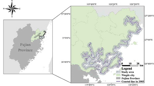
Ningde is located between 118°32′~120°43′E and 26°18′~27°40′N in Fujian Province, Southeast China. Its coastline is 1046 km in length, ranking first in Fujian Province and provides more than 600 aquatic species for direct and indirect human consumption. Besides, Ningde has a long history of coastal aquaculture production. From 1990 to 2018, the fishery output value in Ningde had grown dramatically from 347.71 million yuan to 24,682.71 million yuan (46.88% of GDP in 2018). Ningde City is a well-known location for coastal aquaculture and plays an important role in China’s coastal aquaculture industry. Additionally, it is located at the core area of China’s 21st-century maritime silk road, which will inevitably change the structure and spatial configuration of coastal aquaculture ecosystems.

Coastal region is a buffer zone centered on the coastline and extended to a certain extent of land and sea. There is no unified standard for the division of coastal regions. Researchers can set a reasonable scope according to research needs and local conditions (Finkl 2004). To cover the coastal aquaculture area in Ningde, we followed Liu (2011) and defined a 2 km buffer zone along the coastline in 2003 toward both the land and the sea (in total, a 4 km wide belt along the coastline). Our study area includes the total of four coastal counties of Ningde: Jiaocheng, Xiapu, Fu’an, and Fuding, covering a total area of 2286.25 km² (Figure 1). The aquaculture production of these four cities accounted for 21%, 44.9%, 10%, and 21.5% of Ningde’s total aquaculture production, respectively (Ningde Statistic Bureau 2020).

Figure 1. Study area

Data sources

We collected SPOT-5 and GF-1 satellite images with high resolution of 2.5 m and 2 m to detect changes of coastal aquaculture area in the Ningde coastal region. China’s coastal areas continued to carry out large-scale coastal reclamation after 2000, and this trend increased sharply after 2005 (Tian et al. 2016). So we obtained five SPOT-5 images in 2003, five SPOT-5 images in 2010, and seven GF-1 images in 2016 from China Center for Resources Satellite Data and Application (see Appendix A). These images have been geographically corrected and radiometrically calibrated. Meanwhile, we obtained the Digital Elevation Model (DEM) data (30 m resolution) in the Ningde coastal region from the U.S. Geological Survey. We used ENVI (version 5.3, Exelis Visual Information Solutions) for image geoprocessing. Previous studies have shown that constructed land and huge economic return to local governments may be the direct driving factors of coastal aquaculture (Bostock et al. 2016; Bouwman et al. 2013; Meng et al. 2017; Tantipisanuh, Gale, and Round 2016). To generate geographical indicators as potential driving factors for changes in aquaculture reclamiation, we calculated the Euclidean distances from the centroid of each patch to initial road in 2003, the newly-built road, initial coastline in 2003, initial coastal aquaculture in 2003, newly-built port, newly-built factory, and so forth in ArcGIS (version 10.2, Environmental Systems Research Institute) (Tian et al. 2016).

Change detection of the Ningde coastal region

Object-oriented classification

We carried out the object-oriented classification of coastal aquaculture area using Ecognition (version 9.0, Definiens Imaging). The extraction process mainly consists of three parts: image segmentation, rule establishment, and vector output. First, we used all the bands of the remote sensing image (red, green, blue, and infrared), as well as the Normalized Difference Water Index (NDWI), Normalized Difference Vegetation Index (NDVI), and Normalized Difference Soil Index (NDSI) as input data sets. Second, we adopted the multi-scale segmentation method (Zhang et al. 2013) to create image objects. The results of multi-resolution segmentation are mainly affected by scale parameters, shape, and compactness. Through experiment and error analysis, we set the segmentation scale, shape factor, and compactness factor as 10, 0.2, and 0.8, respectively (Benz et al. 2004; Flanders, Hallbeyer, and Pereverzoff 2003; Incekara, Seker, and Bayram 2018). Then, on the basis of field investigation and image training area analysis, we constructed the decision tree rules (waterbody:NDWI > 0.45, woodland: NDVI > 0.20, constructed land: NDVI < 0, NDWI < 0.20, farmland: 0.20 > NDVI > 0, coastal aquaculture: 0.45 > NDWI > 0.20, bare land: NDSI < −0.05, Elevation > 50) (Incekara, Seker, and Bayram 2018). Furthermore, using ground survey data and Google Earth photos as training samples, we adopted the nearest neighbor classifier method to classify other land cover types. Finally, we exported the classification results into shapefiles. The extraction rule thresholds of images with different acquisition dates are different, and the classification parameters were optimized according to the characteristics of the image manually. We performed the accuracy assessment using 1000 points randomly generated in each of the year in 2003, 2010, and 2016, respectively. We finally classified our study area into seven land-use types: coastal aquaculture (CA), constructed land (CL), bare land (BL), farmland (FL), waterbody (WB), woodland (WL), and other land (OL) (Figure 2). We used ArcGIS (version 10.2, Environmental Systems Research Institute) to display the spatiotemporal pattern, and Fragstats (version 4.2, Oregon State University) and Stata (version 14.0, StataCorp, Texas) for further quantitative analyses.

Figure 2. Procedures of Ningde coastal region land use and land cover classification

Landscape changes

We used four common measures (i.e., regional change, dynamic landscape degree, landscape change index, and landscape type conversion matrix) (Cheng et al. 2019) to express the coastal landscape change. We calculated the dynamics (K) to measure the regional change rate of the landscape. K refers to the percentage of the annual regional change of the ecosystem compared with the initial ecosystem area (Krajewski, Solecka, and Mastalska-Cetera 2017; Puyravaud 2003):

(1) $\mathrm{K}=\frac{{\mathrm{A}}_{\mathrm{t}+1}-{\mathrm{A}}_{\mathrm{t}}}{{\mathrm{A}}_{\mathrm{t}}}\times \frac{1}{\mathrm{\Delta }\mathrm{t}}\times 100\mathrm{\%}$(1)

K is the percentage of land-use change per year, which indicates the dynamic degree of land use in a particular landscape. A_t and A_t+1 represents the coastal landscape area at time t and t + 1, and Δt represents the duration.

The Landscape Change Index (LCI) is an useful indicator of overall landscape change. LCI is defined as the absolute value of changes in landscape types and has the greatest impact on landscape formation (Krajewski, Solecka, and Mastalska-Cetera 2017):

(2) $|\mathrm{L}\mathrm{C}{\mathrm{I}}_{\mathrm{t}\mathrm{i}}|=\frac{1}{2}\times \sum _{\mathrm{i}}^{\mathrm{n}}\left|\mathrm{C}{\mathrm{A}}_{\mathrm{i}}\right|$(2)

LCI_ti represents the landscape change index for each studied period; |CA_i| indicates the area of each landscape type relative to the total analysis area. The absolute value of the proportional change is calculated by:

(3) $\mathrm{C}{\mathrm{A}}_{\mathrm{i}}=\frac{{\mathrm{S}}_{\mathrm{t}+1}/{\mathrm{s}}_{\mathrm{t}}}{\mathrm{T}\mathrm{A}}$(3)

where CA_i represents the ratio of the changing area of a certain landscape type to the total area of the study area (%), S_t and S_t+1 represent the area of a certain landscape type at the beginning and end of the interval (km²); TA represents the total area of the study area (km²).

Landscape metrics

As an indicator of the socioeconomic process, landscape change can effectively reflect the past changes in coastal areas (Seto and Fragkias 2005). Landscape change can be analyzed using landscape metrics. There are a variety of indicators for landscape change assessments (Forman and Godron 1981). According to the characteristics of our study area, we used seven metrics, including number of patches (NP), patch density (PD), division (DIVISION), largest patch index (LPI), shannon’s diversity index (SHDI), perimeter area fractal dimension (PAFRAC), and contagion index (CONTAG). We selected these metrics to illustrate the overall landscape conditions and the coastal aquaculture pattern changes in Ningde coastal area from 2003 to 2016 (Table 1). We performed the calculation in Fragstats (version 4.2, Oregon State University) (McGarigal and Marks 1995).

Table 1. Description of landscape metrics

Landscape index	Formula
NP	NP = ni; n-Number of patch
PD	PD = N/A; N-Number of patch; A-Total area
LPI	LPI = Max (a1, … an)/A × 100; ai-patch area i; A-Total area
CONTAG	$\mathrm{C}\mathrm{O}\mathrm{N}\mathrm{T}\mathrm{A}\mathrm{G}=\left[1+\frac{{\sum }_{\mathrm{i}=1}^{\mathrm{m}}{\sum }_{\mathrm{k}=1}^{\mathrm{m}}\left[\left({\mathrm{P}}_{\mathrm{i}}\right)\left(\frac{{\mathrm{g}}_{\mathrm{i}\mathrm{k}}}{{\sum }_{\mathrm{k}=1}^{\mathrm{m}}{\mathrm{g}}_{\mathrm{i}\mathrm{k}}}\right)\right]\left[ln({\mathrm{P}}_{\mathrm{i}})\left(\frac{{\mathrm{g}}_{\mathrm{i}\mathrm{k}}}{{\sum }_{\mathrm{k}=1}^{\mathrm{m}}{\mathrm{g}}_{\mathrm{i}\mathrm{k}}}\right)\right]}{2ln\left(\mathrm{m}\right)}\right]\times 100$; pi-The percentage of the area occupied by the type of patch; gik-The number of type I patch adjacent to class k plaques; m-Total number of patch types in the landscape
PAFRAC	$\mathrm{P}\mathrm{A}\mathrm{F}\mathrm{R}\mathrm{A}\mathrm{C}=\frac{\frac{2}{\left[{\mathrm{n}}_{\mathrm{i}\mathrm{j}}{\sum }_{\mathrm{j}=1}^{\mathrm{n}}\left(\mathrm{l}\mathrm{n}{\mathrm{p}}_{\mathrm{i}\mathrm{j}}-ln{\mathrm{a}}_{\mathrm{i}\mathrm{j}}\right)\right]-\left[\left({\sum }_{\mathrm{j}=1}^{\mathrm{n}}{\mathrm{p}}_{\mathrm{i}\mathrm{j}}\right)\left({\sum }_{\mathrm{j}=1}^{\mathrm{n}}{\mathrm{a}}_{\mathrm{i}\mathrm{j}}\right)\right]}}{\left({\mathrm{n}}_{\mathrm{i}}{\sum }_{\mathrm{j}=1}^{\mathrm{n}}ln{\mathrm{p}}_{\mathrm{i}\mathrm{j}}^2\right)-{\left({\sum }_{\mathrm{j}=1}^{\mathrm{n}}ln{\mathrm{p}}_{\mathrm{i}\mathrm{j}}\right)}^2}$; aij-patch area; Pij-patch perimeter; ni-patch number.
$\mathrm{D}\mathrm{I}\mathrm{V}\mathrm{I}\mathrm{S}\mathrm{I}\mathrm{O}\mathrm{N}$	$\mathrm{D}\mathrm{I}\mathrm{V}\mathrm{I}\mathrm{S}\mathrm{I}\mathrm{O}\mathrm{N}=\left[1-\sum _{j=1}^n{\left(\frac{a_{ij}}{A}\right)}^2\right]$; aij-Patch area; A-Total area
SHDI	$\mathrm{S}\mathrm{H}\mathrm{D}\mathrm{I}=-\sum _{\mathrm{i}=1}^{\mathrm{m}}\left({\mathrm{p}}_{\mathrm{i}}\mathrm{l}\mathrm{n}{\mathrm{p}}_{\mathrm{i}}\right)$; Pi-Proportion of land occupied by patch type i; m-Number of patch types present in the landscape

Driving force analysis

We constructed regression models for driving force analysis. The formula can be expressed as follows:

(4) $\mathrm{y}={\beta }_1\mathrm{X}+{\beta }_2\mathrm{T}+\epsilon$(4)

where y is the dependent variable vector of n × 1; n is the number of small coastal aquaculture patches; X is the matrix of driving factors and intercepts of n × k; k is equal to the number of driving factors plus 1 (1 refers to the dimension of the intercept); T is a vector consisting of discrete variables of coastal aquaculture types; β₁ and β₂ are coefficient vectors of k × 1; ε is an error term vector of n × 1.

Driving factors for coastal aquaculture area changes may vary at different scales. Here we selected the 2003 coastline as baseline because it is the earliest available SPOT image we could access in our study area. We then generated grids along the 2003 coastline. We tried different grid width, such as 100 m, 300 m, and 500 m, to perform our driving force analysis. We constructed models for both the growth and attenuation of coastal aquaculture separately. Finally, based on model fitness, coefficient significance, and theoretical analysis, we found 300 m is the best patch width to explain the driving forces for coastal aquaculture.

Results

Spatiotemporal dynamics of the coastal aquaculture

Figure 3 shows the LULCC from 2003 to 2016 in the Ningde coastal region (see details in Appendix B). The overall accuracy of classification for the years of 2003, 2010, and 2016 were 95.60%, 96.70%, and 97.60%, respectively (Appendices C–E). Waterbody, woodland, constructed land, coastal aquaculture, and farmland were the main land-use types, which accounted for 45.16% (1032.51 km²), 37.35% (854.01 km²), 8.08% (184.65 km²), 4.20% (96.08 km²), and 3.68% (84.04 km²) of the total area in 2016. The landscape indices from 2003 to 2016 in the Ningde coastal region show an expansion of coastal aquaculture, constructed land, and woodland, and a shrinkage of waterbody, farmland, and bare land areas. From 2003 to 2010, the dynamics (K) of constructed land was +6.43%, followed by bare land (−5.89%) and farmland (−4.03%). From 2010 to 2016, the dynamics (K) of bare land was −4.74%, followed by constructed land (+4.00%) and farmland (−1.64%). The index of land-use change in 2003–2010 was 1.53, higher than 1.21 in the 2010–2016 period, indicating that landscape changes in 2003–2010 were more intense than those in 2010–2016 (Table 2).

Table 2. Dynamics of landscape changes during 2003–2010 and 2010–2016

Time Interval	Indicator	Ecosystem Types
		CA	CL	BL	FL	WB	WL	OL
2003–2010	K/%	0.29	6.43	−5.89	−4.03	0.02	0.36	3.17
	CA/%	0.08	2.02	−1.46	−1.60	0.07	0.89	0.00
	LCI	1.53
2010–2016	K/%	0.66	4.00	−4.74	−1.64	−0.52	0.31	1.52
	CA/%	0.16	1.56	−0.59	−0.40	−1.46	0.68	0.00
	LCI	1.21

Notes: CA: Coastal aquaculture; CL: constructed land; BL: bare land; FL: farmland; WB: waterbody; WL: woodland; OL: other land.

Figure 3. Land use/cover of the Ningde coastal region in 2003 (left), 2010 (middle), and 2016 (right)

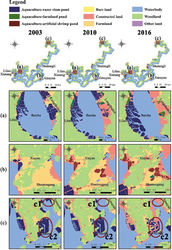
From 2003 to 2016, the growth of coastal aquaculture area in the Ningde coastal region accelerated, and its structure changed significantly. The area of coastal aquaculture increased by 5.99% from 90.65 km² in 2003 (3.97% of the total area) to 96.08 km² in 2016 (4.20% of the total area). Coastal aquaculture expanded to the sea along the coastline, mainly in Xiatang, Lilan, Jimuyan, and Shatangli (Figure 3). Between 2003–2010 and 2010–2016, the area of coastal aquaculture increased by 1.70 km² (1.88%) and 3.73 km² (4.04%), with dynamic degrees (K) of +0.29% and +0.66%, respectively.

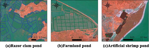
Meanwhile, there were three types of coastal aquaculture, namely razor clam pond, farmland pond, and artificial shrimp pond (Figure 4). The areas of razor clam pond and artificial shrimp pond increased, while the area of farmland pond decreased. Among the three, the growth rate of artificial shrimp pond was the fastest, followed by razor clam pond. From 2003 to 2016, the area of artificial shrimp pond and razor clam pond increased by 496.15% (from 0.52 km² to 3.10 km²) and 12.15% (from 68.78 km² to 77.14 km²), respectively. Meanwhile, the area of farmland pond decreased by 25.81%, from 21.35 km² to 15.84 km².

Figure 4. Types of coastal aquaculture in Ningde coastal region between 2003 and 2016. Razor clam: in blue color; farmland pond: in green color, and artificial shrimp pond: in red color

Land conversion in the coastal aquaculture region

The changes in coastal aquaculture area included growth and reduction, and each mainly has two types: change toward the sea and change toward the inland (Figure 3). The growth of coastal aquaculture area mainly included expansion to the ocean represented by razor clam aquaculture ponds (Figure 3(a)), and expansion toward the inland represented by farmland ponds and artificial shrimp ponds (Figure 3(b)). The decline of coastal aquaculture area mainly includes areas being submerged by sea water and being utilized by artificial construction (Figure 3(c)).

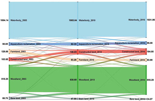
Figure 5 shows the converted areas between different land use types in the coastal aquaculture region from 2003 to 2010 and from 2010 to 2016 (see details in Appendices F and G). Specifically, from 2003 to 2010, the top three main growth sources of coastal aquaculture area were waterbody, farmland, and constructed land, which were 13.96 km², 9.15 km², and 1.60 km², respectively. The attenuation of coastal aquaculture area was mainly converted to waterbody, constructed land, and farmland, which were 11.57 km² 8.00 km², and 3.43 km², respectively. From 2010 to 2016, the top three sources of growth were waterbody, farmland, and constructed land, which were 23.11 km², 5.49 km², and 2.06 km², respectively. The reduced aquaculture areas were mainly replaced by constructed land (14.81 km²), waterbody (6.63 km²), and farmland (4.57 km²), respectively.

Figure 5. Transfer flows of different land use types between 2003–2010 and 2010–2016. See details in Appendices F and G

Landscape pattern change of coastal aquaculture area

Table 3 shows the landscape changes of coastal aquaculture area and the entire Ningde coastal region. Our results revealed that from 2003 to 2016, the change trends of the coastal aquaculture area and the entire Ningde coastal region were consistent, and became more fragmented and dispersive. At the coastal aquaculture area scale, on the one hand, the NP and the PD of coastal aquaculture area patches increased from 2269 to 3390 and from 0.99 to 1.62, respectively, indicating that the landscape became more fragmented. On the other hand, the PAFRAC of coastal aquaculture area patches increased from 1.31 to 1.46, reflecting its shape complexity was enhanced. Moreover, the LPI did not change obviously, suggesting that the dominant coastal aquaculture patches was unchanged. At the regional scale, the NP, the PD, and the DIVISION of the overall landscape pattern increased from 31,903 to 80,692, from 13.75 to 35.47, and from 0.80 to 0.89, respectively, showing that the entire landscape became more fragmented. Besides, the PAFRAC increased from 1.23 to 1.31, indicating the shape complexity of entire landscape increased. Moreover, the CONTAG and SHDI did not change obvious, suggesting that the connectivity of the original superiority patches was basically unchanged.

Table 3. Landscape pattern metrics of the coastal aquaculture area and the entire Ningde coastal region

Place	Indicator	2003	2010	2016
Coastal aquaculture area	NP	2269	3369	3690
	PD	0.99	1.48	1.62
	LPI	0.08	0.04	0.05
	PAFRAC	1.31	1.22	1.46
Ningde coastal region	NP	31,403	63,801	80,692
	PD	13.75	27.93	35.47
	DIVISION	0.80	0.81	0.89
	SHDI	1.27	1.24	1.25
	PAFRAC	1.23	1.30	1.31
	CONTAG	65.15	65.15	64.94

Driving forces for changes in coastal aquaculture area

Table 4 shows the descriptive statistics of variables used in our coastal aquaculture area growth and attenuation models. Our growth model reveals that the initial coastal aquaculture area in 2003, the distance to initial road in 2003, the distance to initial coastal aquaculture area in 2003, the distance to newly-built port and the distance to initial coastline in 2003 were positively correlated with the expansion of coastal aquaculture area (Table 5). Among them, the most significant driving factor was the initial coastal aquaculture area in 2003, followed by the distance to initial aquaculture, and the distance to initial road in 2003. With all other relevant factors controlled at their mean values, an increase of the initial coastal aquaculture area in 2003 by 1 km², the increase of the coastal aquaculture area was 0.29 km². In addition, an increase of the distance to initial road in 2003 by 1 km, the distance to initial coastal aquaculture area in 2003, the distance to newly-built port, the distance to initial coastline in 2003, the increase of the coastal aquaculture areas were 3.84 km², 5.18 km², 2.58 km², and 1.49 km², respectively.

Table 4. Descriptive statistics of variables used in the regression model

Independent variable	Growth model			Attenuation model
	Mean (S.D.)	Mean (S.D.)
Initial coastal aquaculture area in 2003 (ha)	6.832(16.195)		10.724(19.573)
Distance to initial road in 2003 (m)	5.027(1.125)		4.984(1.042)
Distance to initial coastal aquaculture area in 2003 (m)	5.221(1.146)		-
Distance to newly-built port (m)	7.490(0.983)		-
Distance to initial coastline in 2003 (m)	−2.533(4.475)		-
Distance to newly-built factory (m)	-		7.660(1.222)
Distance to newly-built road (m)	-		6.595(1.904)

Notes: The distance variables used in the models are in the natural log form. For the distance to the coastal line in 2003, negative values indicated the direction to the land, and positive values indicated the direction to the sea.

Table 5. Coefficients of factors that are associated with coastal aquaculture area changes

Variable	Growth model		Attenuation model
	Unstandardized coefficient (SE)	Standardized coefficient (SE)	Unstandardized coefficient (SE)	Standardized coefficient (SE)
Initial coastal aquaculture area in 2003	0.290* (0.115)	0.570*** (0.027)	0.364*** (0.072)	0.677*** (0.134)
Distance to initial road in 2003 (log)	10,431.690** (2998.761)	0.142*** (0.028)	10,529.580*** (2251.809)	0.104*** (0.022)
Distance to initial coastal aquaculture in 2003 (log)	14,068*** (3585.648)	0.194*** (0.027)	-	-
Distance to newly-built port (log)	7023.016*** (1628.327)	0.083** (0.026)	-	-
Distance to initial coastline in 2003 (log)	4044.739*** (579.363)	0.218*** (0.029)	-	-
Distance to newly-built factory (log)	-	-	−14,529.370*** (2615.052)	−0.169*** (0.030)
Distance to newly-built road (log)	-	-	−7225.955*** (1940.229)	−0.131*** (0.035)
Intercept	146,004.400*** (20,106.330)	3.790E-9 (0.026)	112,921.500*** (31,230.640)	1.620E-9 (0.026)

Notes: *p < 0.05, **p < 0.01, ***p < 0.001. The growth model: N = 829, R² = 0.449. The attenuation model: N = 582, R² = 0.596. Variance inflation factors were tested to be < 5 in all models (see Appendices H and I).

Our attenuation model shows that the initial coastal aquaculture patch area and the distance to initial road in 2003 showed a positive correlation with the attenuation of coastal aquaculture area (Table 5). Among them, the most significant factor to drive its attenuation was the initial coastal aquaculture area in 2003, followed by the distance to newly-built factory, and the distance to newly-built road. With all other relevant factors controlled at their mean values, an increase of the initial coastal aquaculture area in 2003 by 1 km² and the distance to initial road in 2003 by 1 km would lead to the attenuation of the coastal aquaculture areas by 0.36 km² and 3.87 km², respectively. The distance to newly-built factory and the distance to newly-built road showed a negative correlation with the attenuation of coastal aquaculture area (Table 5). Again, controlling all other relevant variables at their mean values, a decrease of the distance to newly-built factory and the distance to newly-built road by 1 km would lead to the attenuation of the coastal aquaculture areas by 5.34 km² and 3.66 km², respectively.

Discussion

Changes of coastal aquaculture area in Ningde coastal region

China’s coastal aquaculture area has a long history. Since 1980, reclamation in China’s coastal areas mainly shifted from agricultural land to aquaculture ponds (Gao et al. 2014). In Ningde coastal region, coastal aquaculture mainly came from the waterbody and farmland. Such process is consistent with what happened in the Yellow River Delta where aquaculture ponds in the coastal areas from 1983 to 2015 mainly came from coastal wetlands and farmland (Ren et al. 2018). Meanwhile, from 2003 to 2016, we found that the razor clam pond has increased the most, mainly due to its characteristics of the larger area occupancy. At the same time, the artificial shrimp pond had the fastest growth rate, mainly due to its small initial quantity and higher economic return. In addition, the decrease of farmland pond was mainly caused by the sprawl of construction.

The large-scale development of coastal aquaculture ponds has been closely related to the rapid growth of economy, escalating demand of seafood, and expansion of infrastructure construction (Bostock et al. 2016; Bouwman et al. 2013; Tantipisanuh, Gale, and Round 2016). Our study showed that human activities (e.g., road and factory construction) were the main driving factors for changes in coastal aquaculture area. For the growth of coastal aquaculture area, the larger initial coastal aquaculture area meant the higher financial capital and stronger ability to construct more aquaculture infrastructure. Besides, the further away from roads, the less human impacts on aquaculture, and thus the easier for coastal aquaculture area. Furthermore, far away from the initial coastal aquaculture area can effectively alleviated the negative impacts (e.g., water quality) caused by high aquaculture density (Wang et al. 2019). In addition, the further away from the coastline, the larger seascape is available to be reclaimed. For the attenuation of coastal aquaculture area, the area with larger initial reclamation area was easier to decay. It is because the larger initial area not only means more attenuation potential, but also indicates higher investment, maintenance costs, and risks (e.g., typhoon, fish diseases, and market fluctuation) (Barnard et al. 2015). In addition, the further away from roads, the more inconvenient to maintain the coastal aquaculture areas, and thus the easier to be abandoned. Finally, the construction of new roads and factories often directly occupies coastal aquaculture areas, causing immediate decline.

Environmental impacts of coastal aquaculture

The large-scale development of coastal aquaculture also led to severe environmental impacts, ranging from rapid decline and degradation of coastal wetlands to water pollution and wildlife habitat loss. In the 1950s and 1980s, the upsurge of coastal aquaculture in China halved the total area of natural coastal wetlands, causing the sharp decline of fish, shrimp, crab, and shellfish population (Tian et al. 2016). Many rare and endangered wild animals and plants even faced extinction. Furthermore, the expansion of coastal aquaculture, agriculture, and constructed land led to a large amount of mangrove losses, which was essential to coastal ecosystems for food provision, wave mitigation, and wildlife habitat (Hossain, Uddin, and Fakhruddin 2013; Vo et al. 2013). For instance, Seto and Fragkias (2007) calculated the conversion rate between mangrove area and aquaculture development in the Red River Delta (Vietnam) using land satellite images from 1975 to 2002 and found a strong correlation between the increase in aquaculture areas and the decrease in mangrove areas. Coastal aquaculture also gradually destroys the wildlife habitat and threats the species diversity. As an important index of ecosystem quality, the waterfowl population such as the overwintering population of red-crowned crane suffered from a 54.55% decline from over 1100 to less than 500 birds over the last 30 years, and there has been an alarming decline of 50–150 birds per year in recent years (Su and Zou 2012). The growth of the coastal aquaculture area in the coastal region directly turned the coastal bird habitat into aquaculture land and reduced food provision to migratory waterbirds (Yan et al. 2017).

Suggestions for future research and management

To reduce the negative impacts of coastal aquaculture area and sustainably manage the coastal ecosystems, we provide the following recommendations for future research and management. First, it is necessary to take a coupled human and natural systems approach to understanding human-nature interactions within and beyond coastal ecosystems. On one hand, human activities (e.g., coastal aquaculture, infrastructure construction) negatively affect coastal wetlands but enhance socioeconomic benefits. On the other hand, the degradation and decline of coastal wetlands largely reduce the provision of many key ecosystem services (e.g., wave and flood mitigation, water purification, waterbird habitat) and threaten human well-being (Halpern et al. 2012). Second, it is important to conduct an integrated assessment of environmental and socioeconomic impacts of coastal and marine aquaculture (Wang and Yang 2019). Although there are scattered studies on environmental and socioeconomic impacts of coastal and marine aquaculture, the systematical understanding is still largely missing in existing literature. Particularly, existing studies often focus on local impacts and ignore spillover effects in the regional, national, and even global scales (Liu et al. 2015; Liu, Yang, and Li 2016). However, coastal and marine aquaculture involves many telecoupled processes (e.g., feed import, seafood export, and worker migration) whose impacts are so influential and cannot be neglected (Marin et al. 2019). Finally, systematical spatial planning and monitoring of coastal and marine land use is urgently needed. Previous development of coastal and marine aquaculture in China is mostly unregulated and disordered. It is not only difficult for standardized aquaculture operations to ensure food quality and security, but also generates massive water pollution and increases the risks of fish diseases and algae blooming (Stentiford et al. 2012; Sun et al. 2020; Townhill et al. 2018).

Author contributions

W.Y. designed the research; Z.Y. collected and compiled the data, and conducted the analysis; Z.Y. wrote the first draft; all authors revised the manuscript together. The authors declare no competing financial interests.

Acknowledgments

We thank Abdur Hamidi for comments on an earlier draft.

Disclosure statement

No potential conflict of interest was reported by the authors.

Supplementary material

Supplemental data for this article can be accessed here.

Additional information

Funding

We appreciate funding from the National Natural Science Foundation of China [71974171], Ministry of Science and Technology of China [2016YFC0503404], and Outstanding Youth Fund of Zhejiang Province [LR18D010001].

References

- Allison, E. H. 2011. “Aquaculture, Fisheries, Poverty and Food Security.” Working Papers 65: 62.
- Asif, M. B., F. I. Hai, W. E. Price, and L. D. Nghiem. 2018. “Impact of Pharmaceutically Active Compounds in Marine Environment on Aquaculture.” In Sustainable Aquaculture, edited by F. I. Hai, C. Visvanathan, and R. Boopathy, pp. 265–299. Berlin: Springer International Publishing.
- Barnard, P. L., A. D. Short, M. D. Harley, K. D. Splinter, S. Vitousek, I. L. Turner, J. C. Allan, M. Banno, K. R. Bryan, and A. Doria. 2015. “Coastal Vulnerability across the Pacific Dominated by El Niño/Southern Oscillation.” Nature Geoscience 8 (10): 801–12. doi:10.1038/ngeo2539.
- Benz, U. C., P. Hofmann, G. Willhauck, I. Lingenfelder, and M. Heynen. 2004. “Multi-resolution, Object-oriented Fuzzy Analysis of Remote Sensing Data for GIS-ready Information.” Isprs Journal of Photogrammetry and Remote Sensing 58 (3): 239–258. doi:10.1016/j.isprsjprs.2003.10.002.
- Bostock, J., A. Lane, C. Hough, and K. Yamamoto. 2016. “An Assessment of the Economic Contribution of EU Aquaculture Production and the Influence of Policies for Its Sustainable Development.” Aquaculture International 24 (3): 699–733. doi:10.1007/s10499-016-9992-1.
- Bouwman, L., A. Beusen, P. M. Glibert, C. Overbeek, M. Pawlowski, J. Herrera, S. Mulsow, R. Yu, and M. Zhou. 2013. “Mariculture: Significant and Expanding Cause of Coastal Nutrient Enrichment.” Environmental Research Letters 8 (4): 044026. doi:10.1088/1748-9326/8/4/044026.
- Cheng, M., B. Huang, L. Kong, and Z. Ouyang. 2019. “Ecosystem Spatial Changes and Driving Forces in the Bohai Coastal Zone.” International Journal of Environmental Research and Public Health 16 (4): 536–553. doi:10.3390/ijerph16040536.
- Cruz, P. M., A. L. Ibanez, O. M. Hermosillo, and H. R. Saad. 2012. “Use of Probiotics in Aquaculture.” International Scholarly Research Notices 2012 (3): 916845.
- Finkl, C. W. 2004. “Coastal Classification: Systematic Approaches to Consider in the Development of a Comprehensive Scheme.” Journal of Coastal Research 20 (1): 166–213. 10.2112/1551-5036(2004)20[166:CCSATC]2.0.CO;2.
- Flanders, D., M. Hallbeyer, and J. Pereverzoff. 2003. “Preliminary Evaluation of eCognition Object-based Software for Cut Block Delineation and Feature Extraction.” Canadian Journal of Remote Sensing 29 (4): 441–452. doi:10.5589/m03-006.
- Forman, R. T., and M. Godron. 1981. “Patches and Structural Components for a Landscape Ecology.” BioScience 31 (10): 733–740. doi:10.2307/1308780.
- Fuchs, J., J.-L. M. Martin, and J. Populus. 1998. “Assessment of Tropical Shrimp Aquaculture Impact on the Environment in Tropical Countries, Using Hydrobiology, Ecology and Remote Sensing as Helping Tools for Diagnosis.” Rapport final du contrat européen, DRV/RA/RST/98-05, no. 94–284: pp262.
- Gao, Z., X. Liu, J. Ning, and Q. Lu. 2014. “Analysis on Changes in Coastline and Reclamation Area and Its Causes Based on 30-year Satellite Data in China.” Journal of Agricultural Engineering 12: 140–147.
- Halpern, B. S., C. Longo, D. Hardy, K. L. McLeod, J. F. Samhouri, S. K. Katona, K. Kleisner, et al. 2012. “An Index to Assess the Health and Benefits of the Global Ocean.” Nature 488 (7413): 615–620. doi:10.1038/nature11397.
- Han, L., X. Hou, M. Zhu, L. Yu, and M. Gao. 2010. “Study on the Temporal-Spatial Characters of Land-Use Change in the Costal Zone of America in the Latter Half of the 20th Century.” World Regional Studies 19 (2): 42–52.
- Hazarika, M., L. Samarakoon, K. Honda, J. Thanwa, T. Pongthanapanich, K. Boonsong, and K. Luang. 2000. “Monitoring and Impact Assessment of Shrimp Farming in the East Coast of Thailand Using Remote Sensing and GIS.” International Archives of Photogrammetry and Remote Sensing 33: 504–510.
- Hossain, M. S., M. J. Uddin, and A. N. M. Fakhruddin. 2013. “Impacts of Shrimp Farming on the Coastal Environment of Bangladesh and Approach for Management.” Reviews in Environmental Science and Bio\/technology 12 (3): 313–332. doi:10.1007/s11157-013-9311-5.
- Incekara, A. H., D. Z. Seker, and B. Bayram. 2018. “Qualifying the LIDAR-Derived Intensity Image as an Infrared Band in NDWI-Based Shoreline Extraction.” IEEE Journal of Selected Topics in Applied Earth Observations and Remote Sensing 11 (12): 5053–5062. doi:10.1109/JSTARS.2018.2875792.
- Jia, M., M. Liu, Z. Wang, D. Mao, C. Ren, and H. Cui. 2016. “Evaluating the Effectiveness of Conservation on Mangroves: A Remote Sensing-based Comparison for Two Adjacent Protected Areas in Shenzhen and Hong Kong, China.” Remote Sensing 8 (8): 627–647. doi:10.3390/rs8080627.
- Krajewski, P., I. Solecka, and B. Mastalska-Cetera. 2017. “Landscape Change Index as a Tool for Spatial Analysis.” Materials Science and Engineering 245 (7): 1–7.
- Liu, J., H. A. Mooney, V. Hull, S. J. Davis, J. Gaskell, T. W. Hertel, J. Lubchenco, K. C. Seto, P. H. Gleick, and C. Kremen. 2015. “Systems Integration for Global Sustainability.” Science 347 (6225): 1258832. doi:10.1126/science.1258832.
- Liu, J., W. Yang, and S. Li. 2016. “Framing Ecosystem Services in the Telecoupled Anthropocene.” Frontiers in Ecology and the Environment 14 (1): 27–36. doi:10.1002/16-0188.1.
- Liu, T. 2011. The Ecological Safety Assessment and Protection Strategy Analysis Based on GIS in the Coastal Zone of Hainan Island. Xiangtan: Hunan University of Science and Technology.
- Marin, T., J. Wu, X. Wu, Z. Ying, Q. Lu, Y. Hong, X. Wang, and W. Yang. 2019. “Resource Use in Mariculture: A Case Study in Southeastern China.” Sustainability 11 (5): 1396–1417. doi:10.3390/su11051396.
- McGarigal, K., and B. J. Marks. 1995. FRAGSTATS: Spatial Pattern Analysis Program for Quantifying Landscape Structure. Portland: US Department of Agriculture, Forest Service, Pacific Northwest Research Station.
- Meng, W., B. Hu, M. He, B. Liu, X. Mo, H. Li, Z. Wang, and Y. Zhang. 2017. “Temporal-spatial Variations and Driving Factors Analysis of Coastal Reclamation in China.” Estuarine Coastal and Shelf Science 191: 39–49. doi:10.1016/j.ecss.2017.04.008.
- Muttitanon, W., and N. Tripathi. 2005. “Land Use/land Cover Changes in the Coastal Zone of Ban Don Bay, Thailand Using Landsat 5 TM Data.” International Journal of Remote Sensing 26 (11): 2311–2323. doi:10.1080/0143116051233132666.
- Nguyen, -H.-H., C. McAlpine, D. Pullar, K. Johansen, and N. C. Duke. 2013. “The Relationship of Spatial–temporal Changes in Fringe Mangrove Extent and Adjacent Land-use: Case Study of Kien Giang Coast, Vietnam.” Ocean & Coastal Management 76: 12–22. doi:10.1016/j.ocecoaman.2013.01.003.
- Ningde Statistic Bureau. 2020. Ningde Statistical Yearbook 2019. Xiangtan: China Statistics Press.
- Ottinger, M., K. Clauss, and C. Kuenzer. 2016. “Aquaculture: Relevance, Distribution, Impacts and Spatial Assessments–a Review.” Ocean & Coastal Management 119: 244–266. doi:10.1016/j.ocecoaman.2015.10.015.
- Puyravaud, J. P. 2003. “Standardizing the Calculation of the Annual Rate of Deforestation.” Forest Ecology and Management 177 (3): 593–596. doi:10.1016/S0378-1127(02)00335-3.
- Ren, C., Z. Wang, B. Zhang, L. Li, L. Chen, K. Song, and M. Jia. 2018. “Remote Monitoring of Expansion of Aquaculture Ponds along Coastal Region of the Yellow River Delta from 1983 to 2015.” Chinese Geographical Science 28 (3): 430–442. doi:10.1007/s11769-017-0926-2.
- Seto, K. C., and M. Fragkias. 2005. “Quantifying Spatiotemporal Patterns of Urban Land-use Change in Four Cities of China with Time Series Landscape Metrics.” Landscape Ecology 20 (7): 871–888. doi:10.1007/s10980-005-5238-8.
- Seto, K. C., and M. Fragkias. 2007. “Mangrove Conversion and Aquaculture Development in Vietnam: A Remote Sensing-based Approach for Evaluating the Ramsar Convention on Wetlands.” Global Environmental Change-human and Policy Dimensions 17 (3): 486–500. doi:10.1016/j.gloenvcha.2007.03.001.
- Shi, L., F. Liu, Z. Zhang, X. Zhao, B. Liu, J. Xu, Q. Wen, L. Yi, and S. Hu. 2015. “Spatial Differences of Coastal Urban Expansion in China from 1970s to 2013.” Chinese Geographical Science 25 (4): 389–403. doi:10.1007/s11769-015-0765-y.
- Stentiford, G. D., D. M. Neil, E. J. Peeler, J. D. Shields, H. J. Small, T. W. Flegel, J. M. Vlak, B. Jones, F. Morado, and S. M. Moss. 2012. “Disease Will Limit Future Food Supply from the Global Crustacean Fishery and Aquaculture Sectors.” Journal of Invertebrate Pathology 110 (2): 141–157. doi:10.1016/j.jip.2012.03.013.
- Su, L., and H. Zou. 2012. “Status, Threats and Conservation Needs for the Continental Population of the Red-crowned Crane.” Chinese Birds 3 (3): 147–164. doi:10.5122/cbirds.2012.0030.
- Sun, X., B. Chen, B. Xia, Q. Li, and K. Qu. 2020. “Impact of Mariculture-derived Microplastics on Bacterial Biofilm Formation and Their Potential Threat to Mariculture: A Case in Situ Study on the Sungo Bay, China.” Environmental Pollution 262: 114336. doi:10.1016/j.envpol.2020.114336.
- Tantipisanuh, N., G. A. Gale, and P. D. Round. 2016. “Incidental Impacts from Major Road Construction on One of Asia’s Most Important Wetlands: The Inner Gulf of Thailand.” Pacific Conservation Biology 22 (1): 29–36. doi:10.1071/PC15028.
- Tian, B., W. Wu, Z. Yang, and Y. Zhou. 2016. “Drivers, Trends, and Potential Impacts of Long-term Coastal Reclamation in China from 1985 to 2010.” Estuarine, Coastal and Shelf Science 170: 83–90. doi:10.1016/j.ecss.2016.01.006.
- Townhill, B. L., J. Tinker, M. Jones, S. Pitois, V. Creach, S. D. Simpson, S. Dye, E. Bear, and J. K. Pinnegar. 2018. “Harmful Algal Blooms and Climate Change: Exploring Future Distribution Changes.” ICES Journal of Marine Science 75 (6): 1882–1893. doi:10.1093/icesjms/fsy113.
- Vo, Q., N. Oppelt, P. Leinenkugel, and C. Kuenzer. 2013. “Remote Sensing in Mapping Mangrove Ecosystems-An Object-Based Approach.” Remote Sensing 5 (1): 183–201. doi:10.3390/rs5010183.
- Wang, W., H. Liu, Y. Li, and J. Su. 2014. “Development and Management of Land Reclamation in China.” Ocean & Coastal Management 102: 415–425. doi:10.1016/j.ocecoaman.2014.03.009.
- Wang, X., T. Zhou, Z. Ying, J. Wu, and W. Yang. 2019. “Analyses of Water Quality and Driving Forces in Ningde Aquaculture Area.” Acta Ecologica Sinica 40 (5): 1766–1778.
- Wang, X., and W. Yang. 2019. “Water Quality Monitoring and Evaluation Using Remote Sensing Techniques in China: A Systematic Review.” Ecosystem Health & Sustainability 5 (1): 47–56. doi:10.1080/20964129.2019.1571443.
- Xie, H., and W. Gao. 2011. “Land Use/cover Change and Driving Force Analysis of Lianyungang Coastal Zone.” Marine Science 35 (11): 52–57.
- Yan, F., N. Li, W. Yang, Y. Qiao, and S. An. 2017. “Effects of Reclamation on Wetland Waterbird Populations, Behaviors and Habitats.” Chinese Journal of Ecology 36 (7): 2045–2051.
- Yao, Y., C. Ren, Z. Wang, C. Wang, and P. Deng. 2016. “Monitoring of Salt Ponds and Aquaculture Ponds in the Coastal Zone of China in 1985 and 2010.” Wetland Sci 14: 874–882.
- Zhang, C., and Z. Zhao. 2015. “Temporal and Spatial Change of Land Use/Cover and Quantitative Analysis on the Driving Forces in the Yellow River Delta.” Acta Scientiarum Naturalium Universitatis Pekinensi 51 (1): 151–158.
- Zhang, X., P. Xiao, X. Song, and I. She. 2013. “Boundary-constrained Multi-scale Segmentation Method for Remote Sensing Images.” Isprs Journal of Photogrammetry & Remote Sensing 78 (4): 15–25. doi:10.1016/j.isprsjprs.2013.01.002.