Distribution of eight heavy metals in the inner shelf sediments of East China Sea: Risk assessments and sources analysis

ABSTRACT

Although numerous studies on heavy metals (HMs) in sediments have been carried out in the East China Sea (ECS), the knowledge on the recent pollution levels of HMs in coastal region remains not well understood due to the rapid developments of urbanization in eastern China. In this study, 23 surface samples and 4 core samples are collected in the inner shelf of the ECS. The average dry-weight concentrations follow the descending order of Zn, Cr, Ni, Pb, Cu, As, Cd, and Hg (103.6 ± 26.0, 42.8 ± 12.4, 37.0 ± 9.1, 34.7 ± 11.1, 19.5 ± 10.3, 15.7 ± 11.6, 0.056 ± 0.017, and 0.041 ± 0.017 μg g⁻¹, respectively). HMs concentrations share a similar spatial distribution pattern of TOC content with a decreasing trend from coastline to outer sea. Additionally, HMs concentrations exhibit a decreasing trend from top to bottom sediments, especially for Hg at the open sites due to the wet and dry deposition of atmospheric Hg besides the riverine inputs. The potential ecological risk indices (PERI) values in coastal sediments were about 2–4 times higher than those in open sea. Although the Hg and Cd concentrations were lower by 2–3 orders of magnitude than those of other six metals, the PERI values of Hg (65.5) and Cd (52.1) were 3–40 times higher than those of others. The hierarchical cluster result is consistent with the PCA result, suggesting that Hg, Cd, and As have similar sources and probably mainly originated from anthropogenic emissions.

KEYWORDS:

• Heavy metals
• spatial distribution
• cores
• environmental risk
• east China Sea

Introduction

Most of heavy metals (HMs) are highly toxic, persistent, and non-degradable contaminants, and more seriously, some species (e.g., mercury (Hg)) are readily enriched in aquatic organisms, and then become a permanent threat to life (Choy et al. 2009; Jeong et al. 2021; Rubalingeswari et al. 2021). HMs in coastal marine environments originated from various sources, including river discharges, surface runoff, and atmospheric deposition (Liu et al. 2018; Xu et al. 2014; Meng et al. 2019). The accumulation of HMs in the marine environment is a critical problem and a serious threat to aquatic organisms and directly or indirectly to human health (Han et al. 2017; Kahal et al. 2018). For example, divalent Hg can be converted into methylmercury, a bioavailable neurotoxin that can jeopardize human health through biomagnification in the food chain. After entering coastal waters, HMs tend to be adsorbed and accumulated in sediments as opposed to water or suspended solids (Han et al. 2017), and thus sediments are usually the ultimate sink for HMs in the marine environment and can be used as a medium to evaluate the contamination of HMs (Selin 2009; Pan and Wang 2012).

In the past four decades, China has experienced substantial industrialization and economic growth since the initiation of reform and opening-up in the late period of 1978. However, the effects of vast development of China on HMs input to the Chinese marginal seas and the potential risks of HMs are still not well understood. The East China Sea (ECS) is close to one of the most developed regions (i.e., Yangtze River Delta, YRD) in China and have subjected to HMs contamination due to the rapid economic and industrial development, especially for Shanghai City and Zhejiang province (Shanhai Statistical Yearbook 2019; Zhejiang Statistical Yearbook 2020). There are numerous harbors, shipyards, and many kinds of industries in the YRD, resulting in large amounts of pollutants being discharged into the rivers and coastal waters of the ECS. A lot of research on HMs in inner shelf of the ECS (including the Yangtze River Estuary (YRE)) has been reported (Fang et al. 2009; Pan and Wang 2012; Duan et al. 2014; Wang et al. 2015; Han et al. 2017; Zhang, Sun, and Xu 2020). Although the concentrations, distributions, and sources of Hg have been studied in the ECS (Shi et al. 2005; Fang and Chen 2010; Meng et al. 2014, 2019; Kim et al. 2018; Cheng et al. 2019; Sun et al. 2020), the levels, distribution characteristics, and ecological risks of other elements (e.g., zinc (Zn), chromium (Cr), nickel (Ni), lead (Pb), copper (Cu), arsenic (As), cadmium (Cd)) in inner shelf of the ECS are not well understood. The lack of this information restrains evaluations of toxic metal pollution in the ECS. Therefore, carrying out in-depth investigations of sedimentary HMs in coastal areas of the ECS remains important. Additionally, ascertaining the distribution patterns and identifying the sources and dominant species of HMs are essential to develop a scientific pollution control strategy.

The objectives of this study are to: (1) ascertain the contamination levels and distributions of eight HMs (i.e., Zn, Cr, Ni, Pb, Cu, As, Cd, and Hg) in the inner shelf of ECS; (2) evaluate the ecological risks of these HMs using both the geo-accumulation index (I_geo) and potential ecological risk index (PERI) methods; and (3) identify the dominant HM species and explore their potential sources.

Materials and methods

Study region and sites

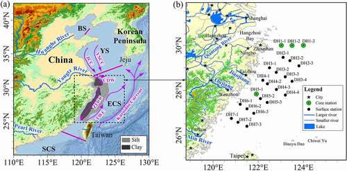
The ECS is a typical marginal sea in the western Pacific Ocean. As illustrated in Figure 1a, it is adjacent to the most developed areas in east China. The coast of the west ECS is one of the most highly developed zones in China. There are many developed cities along the coast, such as Shanghai, Hangzhou, Ningbo, Taizhou, Wenzhou, and Fuzhou (Figure 1b), resulting in a large number of factories in this region. The ECS has received considerable loads of pollutants (including HMs) (e.g., Hg, Liu et al. 2016), causing a variety of environmental problems. Recent rapid economic development and industrialization in east China have resulted in the significant deposition of anthropogenic HMs into the coastal ECS (Chen et al. 2019). Additionally, the ECS is greatly influenced by the Yangtze River, which is the fourth largest river in the world in terms of sediment discharge, about 1.36 × 10⁸ tons was discharged into the ECS annually (Yang et al. 2018 and references therein), and most of Yangtze River-derived sediments and associated pollutants were trapped in the YRE and Zhejiang-Fujian coastal regions due to the sea and ocean currents (Figure 1a). The annual Hg that is exported from mainland China to the ECS was 144 Mg (~70% from anthropogenic sources), which was much higher than those to the Bohai Sea, Yellow Sea, and South China Sea (Liu et al. 2016). Previous studies show that mud (clay and silt) content displayed a band-type distribution in the inner shelf along Zhejiang and Fujian provinces (Hu et al. 2012; Meng et al. 2014 and references therein). The detailed locations of our sampling sites can be found in Table S1 and Figure 1b.

Figure 1. Maps showing the regional sea circulation patterns and surface sediment particle size distribution (modified after Hu et al. 2012; Zhu et al. 2012; Meng et al. 2014) in the ECS (a), and locations of the surface and core sampling sites in inner shelf of the ECS (b). Note that BS: Bohai Sea; YS: Yellow Sea; SCS: South China Sea; TWC: Taiwan Warm Current; CDW: Changjiang (i.e., Yangtze River) Dilute Water; ZFCC: Zhejiang-Fujian Coastal Current; YSCC: Yellow Sea Coastal Current; and JCC: Jiangsu Coastal Current

Sampling method

Twenty-three surface sediments (0–2 cm) and four sediment cores (see Figure 1b) were collected using a gravity corer on the research vessel (Kexue III) during June–July 2013. The previous results of grain sizes of sediments in the ECS (Meng et al. 2014 and references therein) were referenced in this study. Cores DH1-1 and DH5-1 are located in coastal clay area with a water depth of 52.0 and 54.8 m, respectively; cores DH1-2 and DH1-3 are located in the inner shelf with a water depth of 69.0 and 62.9 m, respectively. Immediately after collection, the sediment cores were sliced using a Teflon circle at 2 cm intervals, and then they were wrapped in aluminum foil and then stored in cleaned polyethylene bags, sealed, and refrigerated at −20°C on the research vessel. Upon arrival at the laboratory, all sediment samples were freeze-dried at −45°C for at least 2 days, ground, and homogenized using a pre-cleaned agate mortar and pestle. It is worth noting that stones, dead material of plants, animals, and shells were removed carefully using plastic tweezers, and finally the sediments were sieved through a 100 mesh nylon sieve for later analysis (Duan et al. 2015; Xiao et al. 2017; Cheng et al. 2019).

Determination of heavy metals and total organic matter in sediment

The sediment samples were analyzed for Hg content utilizing direct mercury analyzer (DMA-80, Milestone, Italy). The DMA-80 is based on the principles of sample thermal decomposition, Hg amalgamation, and atomic absorption detection. Quality assurance and quality control were carried out using a system of method blanks, replicates, and standard reference material (SRM) (GBW-07452 (GSS-23), Beijing, China, the Center of National Standard Reference Material of China). Instrument calibration curves covering the appropriate concentrations were checked by the SRM every 10 samples. The measured average THg concentration of GSS-23 (58.9 ± 1.4 ng g^‒1, n = 9) compared favorably with the certified value (58 ± 5 ng g^‒1). Standards varied little over time and were within the calibrated ranges, and the recoveries of certified standards ranged from 94% to 109% (n = 9). The relative percentage difference for the duplicate samples was <15% (6 pairs). Moreover, total organic carbon (TOC) and total organic nitrogen (TON) contents in sediments were also determined using an elemental analyzer (Model: Vario EL III, Germany).

Additionally, 0.2 g (to the accuracy of 0.0001 g) sediment and SRM (GBW-07452) samples were microwave-digested with a mixture of hydrofluoric acid and aqua regia in Teflon vessels. The digested samples were then placed on a hot plate to dry. After that, the residue was solubilized with 2 ml HNO₃ and transferred to a cleaned 50 ml volumetric flask and made up to volume with extracting Milli-Q water (>18.2 MΩ·cm^‒1), and then was centrifuged at a speed of 4000 rpm for 5 min (Fang et al. 2009; Han et al. 2017; Kim et al. 2018; Cheng et al. 2019). Finally, the clear supernatant was analyzed for trace metals (Zn, Cr, Ni, Pb, Cu, As, and Cd) using an inductively coupled plasma mass spectrometer (ICP-MS). Standard quality assurance and control procedures were followed during the analysis of these metals. For each sample batch (10 samples), one method blank and one certified reference material were included. Replicates and the SRM (GBW-07452) were used for quality control protocols. The calibration curve included five concentrations of the seven metals (r² > 0.99 for all the metal species). The relative standard deviation of replicate sample analyses was generally <8% of the mean concentration (n = 9). The recoveries of Zn, Cr, Ni, Pb, Cu, As, and Cd are 101–117%, 82–98%, 96–114%, 104–114%, 95–107%, 102–118%, and 85–105%, respectively (n = 6). The detect limit of Zn, Cr, Ni, Pb, Cu, As, and Cd are 4.7, 0.65, 0.43, 0.24, 0.31, 0.75, and 0.018 μg g⁻¹, respectively, based on three times the standard deviation of the system blanks (n = 6).

Risk assessments of heavy metals in sediments

Methods of geo-accumulation index and potential ecological risk

Toxic metal concentrations in sediments can be used to assess their ecological risk. The geo-accumulation index (I_geo) method proposed by Müller (1969) has been widely adopted to evaluate the contamination levels of HMs in sediments in terms of their corresponding background values. I_geo can be calculated by Equation (1)(1) $I_{geo}={log}_2\left(\frac{C^i}{1.5C_n^i}\right)$(1) :

(1) $I_{geo}={log}_2\left(\frac{C^i}{1.5C_n^i}\right)$(1)

where $C^i$is the measured concentration of heavy metal i, while $C_n^i$ is the geochemical background value of heavy metal i. The background values of Zn, Cr, Ni, Pb, Cu, As, Cd, and Hg in the ECS are 66, 61, 25, 21, 14, 8, 0.032, and 0.025 μg g⁻¹, respectively (Chi and Yan 2007). The classification of the I_geo index, according to Müller (1969), is summarized in Table S2. In the potential ecological risk index (PERI) method, not only the contamination level of each HM but also their unique toxicities and combined ecological risk are taken into consideration. Therefore, PERI is regarded as an appropriate method to assess ecological risk caused by HMs (Håkanson 1980), and this method has been widely used around the world (Hu et al. 2013; Han et al. 2017; Kahal et al. 2018). The risk index provides a fast and single quantitative value on the potential ecological risk of a given contamination situation in a given water system. The potential ecological risk of an individual HM (e.g., i) ($E_r^i$) can be calculated by Equation (2)(2) $E_r^i=T_r^i\times C_f^i$(2) , where $T_r^i$ is the toxic-response factor for a given toxic metal (Zn = 1, Cr = 2, Ni = Pb = Cu = 5, As = 10, Cd = 30, and Hg = 40), and $C_f^i$ is the contamination factor (see Equation (3)(3) $C_f^i=\frac{C^i}{C_n^i}$(3) ). The PERI is calculated by Equation (4)(4) $PERI=\sum _8^{i=1}E{r}^i$(4) , and the contamination degree (C_d) of the eight HMs is calculated by Equation (5)(5) $C_d=\sum _8^{i=1}{C_f}^i$(5) . Classifications of $E_r^i$, C_d, and PERI are listed in Table S2.

(2) $E_r^i=T_r^i\times C_f^i$(2)

(3) $C_f^i=\frac{C^i}{C_n^i}$(3)

(4) $PERI=\sum _8^{i=1}E{r}^i$(4)

(5) $C_d=\sum _8^{i=1}{C_f}^i$(5)

Data analysis

As a multivariate analytical tool, principal component analysis (PCA) is used in present study to determine the relationships of measured HMs and explore the potential sources. The HMs concentrations of all surface and core sediment samples were used to perform the PCA analysis and the SPSS 22.0 was applied to extract the principal components (PCs). Also, dendrogram for hierarchal clusters analyses (HCA) and Pearson’s correlation coefficients were performed. Additionally, ArcGIS 10.2 was used to visualize the spatial distributions of HMs concentrations and contamination levels. Note that ordinary Kriging interpolation was employed as a predictive method.

Results and discussion

HMs concentrations in the ECS and comparisons with other regions

Table S1 summarizes the concentrations of HMs (i.e., Zn, Cr, Ni, Pb, Cu, As, Cd, and Hg) and TOC content in surface sediments of the inner shelf of the ECS. Figure S1 and Table S1 show that the average concentrations of Zn, Cr, Ni, Pb, Cu, and As in the surface sediments were about 2−3 orders of magnitude as high as those of Cd and Hg. Moreover, the normality of HMs concentrations was evaluated, and the frequency histograms of all HMs exhibit that Cu and As concentrations largely skewed toward the lower ranges with a minor counts of data at the higher ends, while the rest HMs all showed a distinct normal distribution (Fig. S2). The lower concentrations often corresponded to samples collected from relatively open sea, whereas higher concentrations were generally corresponded to coastal samples, which will be discussed more detailedly in Section 3.2.

Table 1 summarizes the comparison between the average HMs levels in this study region with those recorded in other open and coastal sediments from Chinese marginal seas. Results show that the mean concentrations of Zn (103.6 ± 26.0 μg g⁻¹), Ni (37.0 ± 9.1 μg g⁻¹), Pb (34.7 ± 11.1 μg g⁻¹), and Cu (19.5 ± 10.3 μg g⁻¹) in the present study were slightly higher than those in inner and outer shelves of the ECS (Zn, Ni, Pb, and Cu are 60, 26, 27, 15 μg g⁻¹, respectively, Fang et al. 2009) probably due to the more serious pollution in recent years. The HMs levels in this study area were higher than those in unpolluted areas, such as the Weihai coast (11.6–34.0 μg g⁻¹, Li et al. 2017). On the whole, the average concentrations of Zn, Cr, Ni, Pb, Cu, and As were comparable to those recorded in the YRE (7.9–94.3 μg g⁻¹, Zhang et al. 2009; Duan et al. 2014; Han et al. 2017), while the Cd and Hg in this study region were lower than those in the YRE. Compared with those reported in the polluted Jinzhou Bay (BS) (1.5–3699 μg g⁻¹, Wang et al. 2010; Li et al. 2012; Fan, Xu, and Wang 2014) listed in Table 1. The Zn, Pb, Cu, and Cd levels in this study region were much lower, while compared with those reported in the Liaodong Bay and Bohai Bay (BS), the observed concentrations of Zn, Cr, Ni, Pb, Cu, As, and Hg in this region were comparable to those reported in these two bays (Zn (58.7–71.8 μg g⁻¹), Cr (60.8 μg g⁻¹), Ni (22.6 μg g⁻¹), Pb (6.9–31.8 μg g⁻¹), Cu (6.5–20.0 μg g⁻¹), As (8.3–11.4 μg g⁻¹), and Hg (0.04–0.05 μg g⁻¹) (Hu et al., 2012; Lin et al., 2012; Li et al., 2015). These results suggest that the ECS inner shelf was moderately polluted by HMs.

Table 1. Comparison of heavy metals concentrations in surface sediments in the various continental shelves along the coat of China

Sampling region	HMs concentrations (μg g^−1)								TOC (%)	Reference
	Zn	Cr	Ni	Pb	Cu	As	Cd	Hg
Inner shelf of ECS	103.6 ± 26.0	42.8 ± 12.4	37.0 ± 9.1	34.7 ± 11.1	19.5 ± 10.3	15.7 ± 11.6	0.056 ± 0.017	0.041 ± 0.017	0.58 ± 0.16	This study
ECS	60		26	27	15				0.10–0.61	Fang et al. 2009
Yangtze River Estuary, ECS	94.3 ± 23.9	78.9 ± 19.7	31.8 ± 7.2	27.3 ± 55.6	30.7 ± 9.7		0.261 ± 0.125		0.701 ± 0.332	Zhang et al. 2009
Yangtze River Estuary, ECS						11.98		0.11	0.42	Duan et al. 2014
Yangtze River Estuary, ECS	66.9 ± 20.9	34.6 ± 14.8		30.5 ± 11.2	17.5 ± 10.5	7.9 ± 2.6	0.15 ± 0.09	0.05 ± 0.02	0.05 ± 0.02	Han et al. 2017
Western Xiamen Bay, ECS	139 ± 39	74.5 ± 12.1	37.4 ± 25.5	54.0 ± 3.7	44.0 ± 21.0		0.331 ± 0.277			Zhang et al. 2007
Jinzhou Bay, BS	484–3669		13.7–33.9	38.2–341	37.9–886		10.4–290		0.41–3.91	Fan, Xu, and Wang 2014
Jinzhou Bay, BS				41–460	26–400		1.5–64			Wang et al. 2010
Jinzhou Bay, BS	689.4 ± 550.6		43.5 ± 41.4	124.0 ± 89.3	74.1 ± 51.5		26.8 ± 20.7			Li et al. 2012
Liaodong Bay, BS	71.7	46.4	22.5	31.8	19.4	8.3		0.04		Hu et al. 2012
Liaodong Bay (Shuangtaiz)	58.7			6.9	6.5		0.5		0.011	Li et al. 2015
Liaodong Bay (Daliao River)	71.8	60.8	22.6	26.6	20.0	11.4	0.34	0.05		Lin et al. 2012
Liaodong Bay, BS				7.50–26.68	4.76–20.16	5.03–30.98	0.18–0.62	0.04–0.22		Liu et al. 2017
Bohai Bay, BS	49.0 ± 11.4	59.1 ± 5.3		10.9 ± 2.2	11.8 ± 3.6	9.1 ± 1.8	0.62 ± 0.23	0.084 ± 0.012		Liu et al. 2018
Western Bohai Bay, BS	83.6	53.1	31.4	20.5	27.9		0.13			Feng et al. 2011
Southern Bohai Bay, BS	71.7	33.5	30.5	21.7	22.7		0.14			Hu et al. 2013
Coastal Bohai Bay, BS	131	101	40.7	34.7	38.5		0.22			Gao and Chen 2012
BS and YS	65.97	59.06	26.69	23.33	20.3	9.92	0.2	0.02		Xu et al. 2016
Southern YS	93.7			17.8	16.9		0.30	0.024		Yuan et al. 2012
Southern YS	78.4 ± 22.8	77.2 ± 18.5	31.4 ± 8.7	21.8 ± 4.3	20.0 ± 7.9		0.207 ± 0.065			Xu et al. 2018
Weihai coast, YS	34.0 ± 24.6	23.9 ± 15.8		20.0 ± 10.5	11.6 ± 3.7	9.0 ± 4.3	0.14 ± 0.07		0.60 ± 0.35	Li et al. 2017
SCS	87.4 ± 47.7	105 ± 86		23.6 ± 8.9	38.1 ± 24.6		0.40 ± 0.40			Zhu et al. 2011
Pearl River Estuary, SCS	143–150	86–89	40–42	53–60	46					Zhou et al. 2014
Beibu Gulf, SCS						8.1 ± 5.8	0.08 ± 0.14	0.034 ± 0.028	0.45 ± 0.39	Gan et al. 2013

Distributions of heavy metals and associated factors

Spatial distribution of HMs in surface sediments

Figure 2 shows the spatial distributions of HMs in surface sediment. It could be found that the HMs concentrations present a large spatial variability and exhibit a distinct spatial distribution pattern with a decreasing trend from nearshore to the outer sea. For example, the surficial sedimentary Zn concentration varied from 45.6 μg g⁻¹ at the relatively open station HD4-4 to 142.6 μg g⁻¹ at the coastal station DH6-1, and a similar pattern can be found for other HMs. As illustrated in Figure 2, the stations near major industry cities, such as Taizhou, Ningbo, and Wenzhou, exhibit relatively high concentrations. A few stations near the coast of Zhejiang province (e.g., DH3-1, DH4-1, and DH5-1) have HMs concentrations 3–7 times higher than the average concentrations of the ECS, whereas the minimal HMs concentrations were detected in sand-silty sediments (i.e., DH3-4 and DH4-4). It is implied that HMs concentrations in the study region were greatly affected by the land-based discharge and riverine inputs from the Yangtze River and other small rivers (Su et al. 2013; Liu et al. 2016). Previous Pb isotopic analyses showed that more than half of sediment Pb in the ECS originated from anthropogenic sources (Chen et al. 2017; Cheng et al. 2019), and thus we speculate that the proportion of anthropogenic sources (e.g., urban/industrial sewage discharges) in the nearshore area might be higher. Another distinct feature is that the highest HMs concentrations were observed in coastal regions of the Zhejiang province, while the HMs in the east waters of the Hangzhou Bay were relatively lower compared to those on the coast of Zhejiang province. This is mainly caused by the diluting effect of CDW and the higher sedimentation rates in the northern study region compared to the southern inner shelf (Li et al. 2012; Liu et al. 2017).

Figure 2. Spatial distributions of HMs in surface sediments of the study area

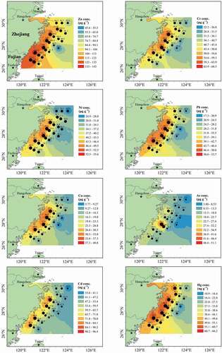
In general, the elevated HMs concentrations extended along the clay area of the inner shelf of the ECS. This indicates that the occurrence of elevated HMs and TOC content in the coastal ECS was closely associated with the input from the rivers (i.e., Yangtze, Qiantang, Jiaojiang, and Oujiang Rivers). This is mainly due to the fact that the spatial distribution of sediment types is closely associated with the sea and/or ocean currents. A large proportion of Yangtze River-derived sediments are transported southwards along the coast driven by the ZFCC and trapped in the inner shelf regions due to the blocking by the northward offshore TWC, and thus an elongated inner-shelf mud wedge is consequently developed from Yangtze mouth to Taiwan Strait (Zhu et al. 2012). This indicates that the accumulation rate of sediments decreased gradually from north to south in the inner shelf region, revealing that coarse particles tend to deposit in estuaries while fine particles can travel longer distances. Therefore, the specific geologic and hydrodynamic features are the dominant factors for the distributions of sediment HMs. Another important reason is that the atmospheric deposition flux of pollutants in nearshore waters was higher than that in the relatively open sea. For example, our previous study showed that the concentration and dry deposition flux of atmospheric particulate Hg were higher in coastal regions than in open sea (Wang et al. 2016a). A recent study reported that contaminated riverine discharge was the dominant Hg source for estuarine and adjacent shelf areas in the ECS based on the isotopic method, whereas precipitation-derived atmospheric deposition had a greater influence on offshore sediment Hg content (Sun et al. 2020). Based on the present and previous studies, we can draw the conclusion that the hydrodynamic conditions and depositional mechanism of the riverine sediments fundamentally control the spatial distribution and fate of Hg in the ECS.

Vertical distribution of sediment HMs

As the previous discussion in Section 3.2.1, the HMs concentrations in nearshore region near Zhejiang province were elevated, so we select core DH5-1 to compare with a coastal core (DH1-1) and an open core (DH1-3). The vertical distributions of the eight HMs, together with the TOC content, for DH1-1, DH1-3, and DH5-1 are illustrated in Figure 3. A striking feature is that there was a larger variation of Zn concentration compared to other HMs. Another distinct feature is that the HMs concentrations (except Cd) at the two coastal sites DH1-1 and DH5-1 varied little in the vertical distribution but a few increase at the top sediments recently (Figure 3a, c). However, as illustrated in Figure 3d–f, the mean concentration of each element at DH1-3 was significantly lower than those at DH1-1 and DH5-1 (t-test, p < 0.01), indicating that the DH1-3 was less polluted. Moreover, it could be found that the Cd concentration decrease from the bottom to the top at the two coastal sites DH1-1 and DH5-1, suggesting the Cd pollution has decreased in recent years. Overall, TOC content and HMs concentrations all exhibit a decreasing trend from the top to the bottom sediments. This vertical pattern is more pronounced for Hg probably due to the wet and dry deposition of atmospheric Hg in addition to the riverine inputs. In addition, as illustrated in Figure 3d–f, the vertical profile data show that the total concentration of HMs in sediments varied greatly in the vertical dimension, indicating that there was some difference in pollution level during different periods. However, it could be found that the concentrations of total HMs in the surface layers were slightly higher than those in the other layers within the depth of 10 cm at these three sites (Figure 3d–f). This further suggests that the surface layer is more polluted than the other layers, in other words, the pollution in recent years was more serious than previous periods. This requires local government to work out HMs pollution control measures as soon as possible, especially in coastal areas.

Figure 3. Depth profiles of HMs and TOC contents for the three sediment cores. Note that the units of Cd and Hg are ng g⁻¹, while the units for other six metals are μg g⁻¹

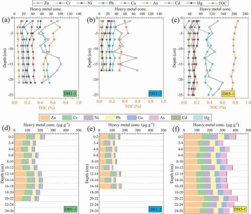
Additionally, in order to compare the distribution characteristics of HMs in a cross section from near shore to open sea, we choose a cross section (i.e., DH1-1, DH1-2, and DH1-3) as a research objective. The results show that the mean Hg concentrations for cores DH1-1, DH1-2, and DH1-3 were 36.6 ± 10.5, 22.9 ± 4.8, 10.9 ± 5.6 ng g⁻¹ with the range of 27.8–57.5, 18.6–31.2, and 5.4–21.4 ng g⁻¹, respectively (Fig. S3). We found that the highest Hg and TOC contents in core DH1-1, followed by core DH1-2, and the lowest values were observed in core DH1-3, representing a decreasing trend from the coast to the open sea. Fig. S3 shows that the Hg concentrations at DH1-1 and DH1-2 decreased from the bottom of the core to the depth at 17 cm, from where it increased gradually to the top, while at DH1-3 the Hg concentration slightly decreased from the surface to the bottom. Additionally, as for the open sea station DH1-3, statistical results show that the Hg values in surface and subsurface sediment were more than two times higher than those in bottom layers, indicating that anthropogenic sources (urban and industrial pollutants) also have a greater impact on the relatively open sea in recent years. Generally, the vertical patterns of TOC content for the three cores were similar and they were all roughly consistent with the distribution of sediment Hg concentration (Figures 3 and S3b). The detailed relationship between Hg and other HMs concentrations and TOC content will be discussed in the next section.

Relationship between HMs concentrations and TOC and TON contents

A variety of sediment properties can influence toxic metals in the sediment, including organic matters. Previous studies show that the levels, speciation, and distributions of HMs in sediment were found to be closely associated with TOC content (Chakraborty et al. 2015; Li et al. 2015). Generally, HMs have a high tendency to be adsorbed onto fine particles with higher organic matters that have a higher surface area (Duan et al. 2015; Cheng et al. 2019). For example, a previous study shows that Hg was most significantly correlated with clay, the next with silt, and finally with sand (Ding et al. 2009). TOC content of these four sediment cores decreased as the following sequence: DH5-1> DH1-1> DH1-2> DH1-3 (Figure 3 and S3). Figure 4 shows the spatial distributions of surface sediment TOC and TON contents in our study region. The mean TOC content was 0.58 ± 0.16% (0.27–0.84%) with the highest value at the coastal site DH5-1 and the lowest value at the open site DH3-4 (Figure 4a). Similarly, the highest and lowest TON values were the same as those of TOC, and the TON contents were in the range 0.029–0.114% with a mean value of 0.069 ± 0.026% (Figure 4b).

Figure 4. Spatial distribution TOC and TON contents in the study region

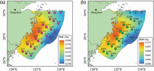
There is a significantly positive relationship between TOC and TON (Table S3). A noteworthy feature is that the TOC and TON content shared greater similarity with HMs concentrations (Figures 2 and 4), and this is consistent with the previous studies conducted in YRE and peripheral areas (Duan et al. 2015; Cheng et al. 2019). Pearson’s results show that not only the eight HMs concentrations are significantly correlated with each other (r > 0.6, p < 0.01) but also they are all significantly positively correlated with the TOC and TON contents (r > 0.7, p < 0.01) (see Table S3 and Fig. S4), indicating that (1) the accumulations of these trace elements in sediments were controlled largely by similar accumulation mechanisms, such as adsorption on particle surfaces or complexation with organic content, (2) TOC was one of the dominant controlling factors for the spatial distribution of HMs. In addition, our previous study showed that the surface seawater total Hg also decreased with distance from the coast toward the outer shelf in the ECS (Wang et al. 2016b), which was consistent with the spatial distributions of the sediment TOC, TON, and HMs concentrations. Moreover, in order to further ascertain the influence of TOC, HMs concentrations are normalized to TOC content. The spatial distribution of HMs/TOC was illustrated in Fig. S5. After normalization, it could be found that there was no significant difference in HMs/TOC values between the coastal region and the relatively open sea (Fig. S5). This further suggests that TOC was a dominant factor for the spatial distribution of HMs.

The above results show that TOC was a key controlling factor for HMs affinity in surface sediment. In order to further ascertain if this rule still worked in the vertical direction, the correlation analysis between TOC and HMs was conducted for cores. There existed significantly positive correlation relationship between TOC and Hg concentrations in the vertical direction for the three sediment cores DH1-1 (r = 0.643, p < 0.05), DH1-3 (r = 0.881, p < 0.01), and DH5-1 (r = 0.586, p < 0.05), which further indicated that TOC was an important parameter controlling Hg distribution. Whereas, as for the coastal core DH1-1, all the HMs except Hg were negatively correlated with TOC content with the r value ranged from −0.141 to −0.824; as for the southern coastal core DH 5–1, half of the HMs (i.e., Ni, Cu, As, and Cr) were negatively correlated with TOC content; while as for the relatively open site DH1-3, all the HMs were positively correlated with TOC content (see Table S4). This probably due to the fact that the coastal sediments were mainly originated from rivers and the sedimentation rate is often influenced by the seasonal variation of river runoff, while the lower and relatively stable sedimentation rate at open sea sites results in a positive correlation between HMs and TOC.

Assessments of environment risks of heavy metals

Geoaccumulation index

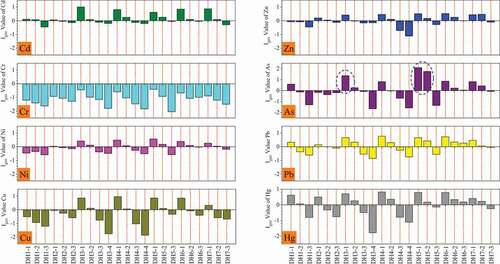
The eight selected HMs in the surface sediments were assessed for potential toxicity using two approaches: I_geo and PERI, which have been widely used to reflect the degree of HMs pollution in sediments. The I_geo values of the eight HMs in surface sediments are shown in figure 5. We found that the I_geo values for Cr are all lower than zero, indicating uncontaminated of this metal species, while only three coastal sites (i.e., DH3-1, DH5-1, and DH5-2) have 1< Igeo<2 for As, indicating moderate As contamination at these sites. A striking feature is that for most of the HMs, except for Cr, the I_geo levels at coastal sites (particularly the DH2-1, DH3-1, DH4-1, DH5-1, DH6-1, and DH7-1) were higher than zero but varied in a narrow range between 0 and 1. Statistical results show that the percentages of samples that had 0< I_geo<1 were 52%, 48%, 61%, 35%, 35%, 57%, and 61% for Zn, Ni, Pb, Cu, As, Cd, and Hg, respectively, indicating slight to moderate contamination. Conversely, as for the relatively open sites, most of the I_geo values for HMs were negative, suggesting light or uncontamination (Figure 5). From the I_geo point of view, most coastal sediment samples in the inner shelf of ECS were slightly-moderately influenced by anthropogenic sources. However, the assessment results may be different when using an evaluation method that considered their respective toxicity indices, see Section 3.3.2.

Figure 5. The I_geo values of the eight HMs for all the surface sediments

Contamination degree and potential ecological risk index of HMs

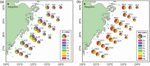
The spatial distributions of C_d and PERI of HMs are illustrated in Figure 6, which shows that both C_d and PERI also display a decreasing gradient from the coast to open sea. The sequence of the average $C_f^i$ values for the eight HMs is As (1.97) > Cd (1.74) > Pb (1.65) > Hg (1.62) > Zn (1.57) > Ni (1.48) > Cu (1.39) > Cr (0.70). Using a $C_f^i$ of 1.0 as the boundary between low contamination and moderate contamination (Table S2), we found that the study region was moderately contaminated by the HMs except Cr, especially for the coastal zone. The mean C_d value was 12.1 ± 4.4 with higher values in the coastal area (particularly the inner shelf near Zhejiang province) and lower values in the relatively open sea (Figure 6a). Based on the contamination assessment criteria (Table S2), the calculated C_d values indicate high contamination levels for the entire area and large polluted areas: approximately 22% of the sites had values of 16< C_d<32, suggesting a considerable degree of contamination, and 61% of the sites had values of 8< C_d<16, suggesting a moderate degree of contamination; whereas only 17% of the sites (mainly located in the relatively open sea) had values of C_d <8, for example, two stations (i.e., DH3-4 and DH4-4) in the open sea had very low C_d values, indicating low contamination status (Figure 6a). Therefore, the contamination levels of these HMs in our study area were established as moderate to considerable from this perspective. However, compared with the standard values of Marine Sedimentary Quality (GB18668–2002, http://openstd.samr.gov.cn/bzgk/gb/), the concentrations of all HMs are slightly lower than the first class value (see Table S5), indicating the relatively low pollution condition in the study region from this perspective. In contrast, the HMs concentrations are significantly higher than the low alert levels (USEPA, 1996; Díaz-de Alba et al. 2011), though they are considerably lower than the high alert level, indicating a certain risks of these HMs.

Figure 6. Spatial distributions of C_d (a) and PERI (b) of HMs in the surface sediments

Although the assessment methods of I_geo and C_d have considered the background values of these HMs, the two approaches also have inherent weaknesses because they give equal importance to all HMs. It is well known that Hg, Cd, and As have higher toxicity compared to the other five selected HMs, and thus even though the concentrations of Hg, Cd, and As were much lower than those of Zn, Cr, Ni, Pb, and Cu, the three high toxicity elements might pose a greater threat to benthic organisms than the others. The PERI method that takes into account both background values and the toxicity of HMs should be more reliable. Fig. S6 shows the spatial distributions of potential ecological risk of each HM ($E_r^i$) in surface sediments of our study area. It could be found that, as illustrated in Fig. S6, the $E_r^i$ values for all HMs shared similar spatial distribution pattern with a decreasing trend from the coast to the open sea as that of HMs concentrations. Moreover, the $E_r^i$ values in the coastal zone were about 2−3 times higher than those in outer shelf area for all elements. There was large difference in $E_r^i$ value between different HMs, and the average $E_r^i$ values of these HMs decreased as following sequence: Hg (65.6 ± 26.1) > Cd (52.1 ± 16.3) > As (19.7 ± 14.5) > Pb (8.3 ± 2.6) > Ni (7.4 ± 1.8) > Cu (7.0 ± 3.7) > Zn (1.6 ± 0.4) > Cr (1.4 ± 0.4). As presented in Fig. S6 and Table S6, all the $E_r^i$ values of Zn, Cr, Ni, Pb, and Cu were much lower than the threshold value (40) of low and moderate ecological risk, and more than 90% of the $E_r^i$ values of As were also lower than this threshold value, while most of the $E_r^i$ values of Hg and Cd were higher than this value. Statistical results show that approximately 78% and 87% of the sampling sites had values of 40 <$E_r^i$<160 for Hg and Cd, respectively, suggesting moderate and considerable ecological risk. Therefore, we can conclude that most of the study areas were moderately polluted by Hg and Cd and they were the dominant pollutants. PERI also shows a decreasing trend from the coastline to the open sea, which was consistent with the C_d values. Figure 6b shows that all PERI values at coastal stations were distributed between 150 and 300, and about 50% of the sampling sites had values of 40< PERI<160, indicating moderate pollution status.

Preliminary analysis of HMs sources

The PCA is conducted for the selected eight HMs to assess their relationships and to identify the possible sources (i.e., anthropogenic sources or natural sources). Figure 7a shows that the studied HMs were concentrated in two zones, indicating that Zn, Cr, Ni, Pb, and Cu might originate from common sources, while Hg, Cd, and As might originate from other similar sources. Table S7 shows that principal component 1 (hereafter referenced as PC1) explains ~75.7% of the total variance of the data set and contains high positive loading for all eight HMs. Especially, the higher PC1 loadings were for Cu, Pb, Ni, Cr, and Zn (all values: >0.85), implying that these metals are generally derived from common sources or accumulated by similar mechanisms. Whereas, principal component 2 (hereafter referenced as PC2) explains ~10.7% of the total variance of the data set and has high loading on Hg, Cd, and As, indicating that these three elements are heavily influenced by similar sources, such as anthropogenic contamination. These demonstrate that both of the PC1 and PC2 are the prominent controlling factors affecting the spatial distribution and concentrations of HMs.

Figure 7. Dendrograms for HCA of eight HMs in surface sediments of the inner shelf of the ECS (a) and principal component loading of HMs (b)

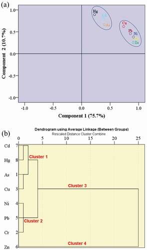
Furthermore, HCA of HMs using average linkage between groups is conducted. The dendrogram derived from the clustering of the studied eight HMs in surface sediment samples is illustrated in Figure 7b. The relations between the eight HMs clustered at different distances were recorded. Two big clusters with subgroups could be distinguished: clusters 1 and 2. The linkage distance between clusters 1 and 2 is very low (2.0), implying a significant linkage between them. Cluster 1 is loaded with four metals (Hg, Cd, As, and Cu) with greater similarity and lower linkage distances, and cluster 2 contains three metals (Cr, Ni, and Pb) with the lowest linkage distance (1.0), while cluster 4 only contains one metal (Zn). Additionally, Figure 7b shows that clusters 1 and 2 are fused at distance 4.0, followed by a fusion of clusters 3 and 4 at a very high distance of 25, indicating that the sources of Zn were quite different from those of other HMs. The results of hierarchical cluster analysis were consistent with the previously defined PCA results. Based on the PCA, hierarchical cluster, and correlation analyses of HMs, we can conclude that Hg, Cd, and As probably mainly originated from anthropogenic sources (urban/industrial sewage discharges), and Zn dominantly originated from natural sources, while other metals probably originated from both anthropogenic and natural sources.

Although this study could not figure out the major sources of sediment HMs and their relative contributions in our study region, previous studies have shown that the elements in sediments of coastal areas of ECS are mainly derived from river inputs (Duan et al. 2013; Chen et al. 2017; Liang et al. 2019). For example, Sun et al. (2020) investigated the sources of HMs based on the isotope-based triple mixing model, and the results show that the major contributors to sediment Hg include industrial discharge (51.8 ± 24.5%), soil Hg from surface runoff (29.2 ± 17.0%), and precipitation-derived atmospheric deposition (19.1 ± 17.5%). Moreover, soil Hg via surface runoff was significant in coastal areas, whereas precipitation-derived atmospheric Hg had a greater influence in offshore regions. Additionally, the stable isotopic ratio of Pb also shows that sedimentary Pb in the coastal areas of the ECS primarily comes from the Yangtze River (Chen et al. 2017). Similar results can be found for As in the nearshore region of the ECS (Duan et al. 2013). Recent studies all reported that Zn and Cr are mainly from natural sources, while As and Cu are mainly imported from fish feed and pesticides produced by humans (Zhai et al. 2021; Zhuang and Zhou 2021). Furthermore, it must be noted that the typhoon can greatly change the vertical (reducing metal concentrations in upper layer sediments) and spatial distributions of HMs in coastal sediments (Wang et al. 2020).

Conclusions

The spatial distributions of HMs in surface sediments corresponded well with the distribution patterns of TOC and TON with a decreasing trend from the nearshore region toward the outer shelf mainly due to the hydrodynamic forces in the inner shelf of the ECS. The higher HMs levels in the coastal area suggest that riverine inputs and land-based discharge played important roles in the distribution of these HMs in surface sediments, which also indicates that the coastal region of the ECS was a major sink of HMs. The observed increasing trend of Hg and Cd concentrations in recent years as recorded in the sediment cores illustrates the escalating use and emission of these two elements. The I_geo, C_d, and PERI also exhibit a clear spatial distribution as those of HMs concentrations. Results show that Zn, Cr, Ni, Pb, and Cu were present at low levels of pollution, and As posed a low to moderate ecological risk, while Hg and Cd posed moderate to considerable ecological risks. What calls for special attention is that the coastal sediments were moderately polluted by HMs, especially for Hg, Cd, and As, and thus it is imperative and urgent to reduce the use and emission of these elements in the Yangtze River Basin and coastal area of the ECS. PCA and hierarchical cluster results revealed that Hg, Cd, and As probably mainly originated from anthropogenic activities, and Zn was dominantly originated from natural sources, while other metals originated from both anthropogenic and natural sources.

Supplemental data

Supplemental data for this article can be accessed here.

Disclosure statement

No potential conflict of interest was reported by the authors.

Correction Statement

This article has been republished with minor changes. These changes do not impact the academic content of the article.

Additional information

Funding

This work was supported by the National Key Research and Development Program of China [2017YFC0505702] and the National Natural Science Foundation of China [41176066, 41807345].

References

- Chakraborty, P., A. Sarkar, K. Vudamala, R. Naik, and B. N. Nath. 2015. “Organic Matter—a Key Factor in Controlling Mercury Distribution in Estuarine Sediment.” Marine Chemistry 173 (2): 302–15. doi:https://doi.org/10.1016/j.marchem.2014.10.005.
- Chen, B., J. Liu, L. Hu, M. Liu, L. Wang, X. Zhang, and D. Fan. 2017. “Spatio-temporal Distribution and Sources of Pb Identified by Stable Isotopic Ratios in Sediments from the Yangtze River Estuary and Adjacent Areas.” The Science of the Total Environment 580: 936–945. doi:https://doi.org/10.1016/j.scitotenv.2016.12.042.
- Chen, L., S. Zhou, S. Wu, C. Wang, and D. He. 2019. “Concentration, Fluxes, Risks, and Sources of Heavy Metals in Atmospheric Deposition in the Lihe River Watershed, Taihu Region, Eastern China.” Environmental Pollution 255: 113301. doi:https://doi.org/10.1016/j.envpol.2019.113301.
- Cheng, Y., R. Zhang, T. Li, F. Zhang, J. Russell, M. Guan, Q. Han, Y. Zhou, X. Xiao, and X. Wang. 2019. “Spatial Distributions and Sources of Heavy Metals in Sediments of the Changjiang Estuary and Its Adjacent Coastal Areas Based on Mercury, Lead and Strontium Isotopic Compositions.” Catena 174: 154–163. doi:https://doi.org/10.1016/j.catena.2018.10.039.
- Chi, Q., and M. Yan. 2007. Handbook of Elemental Abundance for Applied Geochemistry in Chinese. Beijing: Geological Publishing House. 96–97
- Choy, C. A., B. N. Popp, J. J. Kaneko, and J. C. Drazen. 2009. “The Influence of Depth on Mercury Levels in pelagic Fishes and Their Prey.” Proceedings of the National Academy of Sciences U. S. A. 106 (33): 13865–13869. doi:https://doi.org/10.1073/pnas.0900711106.
- Díaz-de Alba, M., M. D. Galindo-Riano, M. J. Casanueva-Marenco, M. García-Vargas, and C. M. Kosore. 2011. “Assessment of the Metal Pollution, Potential Toxicity and Speciation of Sediment from Algeciras Bay (South of Spain) Using Chemometric Tools.” Journal of Hazardous Materials 190 (1–3): 177–187. doi:https://doi.org/10.1016/j.jhazmat.2011.03.020.
- Ding, Z., J. Liu, L. Li, H. Lin, H. Wu, and Z. Hu. 2009. “Distribution and Speciation of Mercury in Surficial Sediments from Main Mangrove Wetlands in China.” Marine Pollution Bulletin 58 (9): 1319–1325. doi:https://doi.org/10.1016/j.marpolbul.2009.04.029.
- Duan, L., J. Song, Y. Yu, H. Yuan, X. Li, and N. Li. 2015. “Spatial Variation, Fractionation and Sedimentary Records of Mercury in the East China Sea.” Marine Pollution Bulletin 101 (1): 434–441. doi:https://doi.org/10.1016/j.marpolbul.2015.09.050.
- Duan, L., J. Song, H. Yuan, X. Li, and N. Li. 2013. “Spatio-temporal Distribution and Environmental Risk of Arsenic in Sediments of the East China Sea.” Chemical Geology 340: 21–31. doi:https://doi.org/10.1016/j.chemgeo.2012.12.009.
- Duan, L., J. Song, H. Yuan, X. Li, N. Li, and J. Ma. 2014. “Distribution, Chemical Speciation and Source of Trace Elements in Surface Sediments of the Changjiang Estuary.” Environmental Earth Sciences 72 (8): 3193–3204. doi:https://doi.org/10.1007/s12665-014-3225-6.
- Fan, W., Z. Xu, and W. Wang. 2014. “Metal Pollution in a Contaminated Bay: Relationship between Metal Geochemical Fractionation in Sediments and Accumulation in a Polychaete.” Environmental Pollution 191: 50–57. doi:https://doi.org/10.1016/j.envpol.2014.04.014.
- Fang, T.-H., and R.-Y. Chen. 2010. “Mercury Contamination and Accumulation in Sediments of the East China Sea.” Journal of Environmental Sciences 22 (8): 1164–1170. doi:https://doi.org/10.1016/S1001-0742(09)60233-3.
- Fang, T.-H., J.-Y. Li, H.-M. Feng, and H.-Y. Chen. 2009. “Distribution and Contamination of Trace Metals in Surface Sediments of the East China Sea.” Marine Environmental Research 68 (4): 178–187. doi:https://doi.org/10.1016/j.marenvres.2009.06.005.
- Feng, H., H. Jiang, W. Gao, M. P. Weinstein, Q. Zhang, W. Zhang, L. Yu, D. Yuan, and J. Tao. 2011. “Metal Contamination in Sediments of the Western Bohai Bay and Adjacent Estuaries, China.” Journal of Environmental Management 92 (4): 1185–1197. doi:https://doi.org/10.1016/j.jenvman.2010.11.020.
- Gan, H., J. Lin, K. Liang, and Z. Xia. 2013. “Selected Trace Metals (As, Cd and Hg) Distribution and Contamination in the Coastal Wetland Sediment of the Northern Beibu Gulf, South China Sea.” Marine Pollution Bulletin 66 (1–2): 252–258. doi:https://doi.org/10.1016/j.marpolbul.2012.09.020.
- Gao, X., and C.-T. A. Chen. 2012. “Heavy Metal Pollution Status in Surface Sediments of the Coastal Bohai Bay.” Water Research 46 (6): 1901–1911. doi:https://doi.org/10.1016/j.watres.2012.01.007.
- Håkanson, L. 1980. “An Ecological Risk Index for Aquatic Pollution Control.a Sedimentological Approach.” Water Research 14 (8): 975–1001. doi:https://doi.org/10.1016/0043-1354(80)90143-8.
- Han, D., J. Cheng, X. Hu, Z. Jiang, L. Mo, H. Xu, Y. Ma, X. Chen, and H. Wang. 2017. “Spatial Distribution, Risk Assessment and Source Identification of Heavy Metals in Sediments of the Yangtze River Estuary, China.” Marine Pollution Bulletin 115 (1–2): 141–148. doi:https://doi.org/10.1016/j.marpolbul.2016.11.062.
- Hu, B., G. Li, J. Li, J. Bi, J. Zhao, and R. Bu. 2013. “Spatial Distribution and Ecotoxicological Risk Assessment of Heavy Metals in Surface Sediments of the Southern Bohai Bay, China.” Environmental Science and Pollution Research 20 (6): 4099–4110. doi:https://doi.org/10.1007/s11356-012-1332-z.
- Hu, L., X. Shi, Z. Yu, T. Lin, H. Wang, D. Ma, Z. Guo, and Z. Yang. 2012. “Distribution of Sedimentary Organic Matter in Estuarine–inner Shelf Regions of the East China Sea: Implications for Hydrodynamic Forces and Anthropogenic Impact.” . Marine Chemistry 142-144: 29–40. doi:https://doi.org/10.1016/j.marchem.2012.08.004.
- Jeong, H., J. Y. Choi, D.-H. Choi, J.-H. Noh, and K. Ra. 2021. “Heavy Metal Pollution Assessment in Coastal Sediments and Bioaccumulation on Seagrass (Enhalus Acoroides) of Palau.” Marine Pollution Bulletin 163: 111912. doi:https://doi.org/10.1016/j.marpolbul.2020.111912.
- Kahal, A. Y., A. S. El-Sorogy, H. J. Alfaifi, S. Almadani, and H. A. Ghrefat. 2018. “Spatial Distribution and Ecological Risk Assessment of the Coastal Surface Sediments from the Red Sea, Northwest Saudi Arabia.” Marine Pollution Bulletin 137: 198–208. doi:https://doi.org/10.1016/j.marpolbul.2018.09.053.
- Kim, J., D. Lim, D. Jung, J. Kang, H. Jung, H. Woo, K. Jeong, and Z. Xu. 2018. “Sedimentary Mercury (Hg) in the Marginal Seas Adjacent to Chinese high-Hg Emissions: Source-to-sink, Mass Inventory, and Accumulation History.” Marine Pollution Bulletin 128: 428–437. doi:https://doi.org/10.1016/j.marpolbul.2018.01.058.
- Li, C., C. Song, Y. Yin, M. Sun, P. Tao, and M. Shao. 2015. “Spatial Distribution and Risk Assessment of Heavy Metals in Sediments of Shuangtaizi Estuary, China.” Marine Pollution Bulletin 98 (1–2): 358–364. doi:https://doi.org/10.1016/j.marpolbul.2015.05.051.
- Li, H., X. Kang, X. Li, Q. Li, J. Song, N. Jiao, and Y. Zhang. 2017. “Heavy Metals in Surface Sediments along the Weihai Coast, China: Distribution, Sources and Contamination Assessment.” Marine Pollution Bulletin 115 (1–2): 551–558. doi:https://doi.org/10.1016/j.marpolbul.2016.12.039.
- Li, X., L. Liu, Y. Wang, G. Luo, X. Chen, X. Yang, B. Gao, X. He, X. He, and J. A. Gilbert. 2012. “Integrated Assessment of Heavy Metal Contamination in Sediments from a Coastal Industrial Basin, NE China.” PLoS ONE 7 (6): e39690. doi:https://doi.org/10.1371/journal.pone.0039690.
- Liang, J., J. Liu, G. Xu, and B. Chen. 2019. “Distribution and Transport of Heavy Metals in Surface Sediments of the Zhejiang Nearshore Area, East China Sea: Sedimentary Environmental Effects.” Marine Pollution Bulletin 146: 542–551. doi:https://doi.org/10.1016/j.marpolbul.2019.07.001.
- Lin, C., M. He, S. Liu, and Y. Li. 2012. “Contents, Enrichment, Toxicity and Baselines of Trace Elements in the Estuarine and Coastal Sediments of the Daliao River System.” Chinese Journal of Geochemistry 46: 371–380.
- Liu, L., L. Wang, Z. Yang, Y. Hu, and M. Ma. 2017. “Spatial and Temporal Variation of Heavy Metals in Marine Sediments from Liaodong Bay, Bohai Sea in China.” Marine Pollution Bulletin 124: 228–233.
- Liu, M., L. Chen, X. Wang, W. Zhang, Y. Tong, L. Ou, H. Xie, et al. 2016. “Mercury Export from Mainland China to Adjacent Seas and Its Influence on the Marine Mercury Balance.” Environmental Science & Technology 50: 6224–6232.
- Liu, Q., F. Wang, F. Meng, L. Jiang, G. Li, and R. Zhou. 2018. “Assessment of Metal Contamination in Estuarine Surface Sediments from Dongying City, China: Use of a Modified Ecological Risk Index.” Marine Pollution Bulletin 126: 293–303.
- “Marine Sedimentary Quality of China (GB18668−2002).”
- Meng, M., J. Shi, Z. Yun, Z. Zhao, H. Li, Y. Gu, J. Shao, B. Chen, X. Li, and G. Jiang. 2014. “Distribution of Mercury in Coastal Marine Sediments of China: Sources and Transport.” Marine Pollution Bulletin 88 (1): 347–353.
- Meng, M., R. Sun, H. Liu, B. Yu, Y. Yin, L. Hu, J. Shi, and G. Jiang. 2019. “An Integrated Model for Input and Migration of Mercury in Chinese Coastal Sediments.” Environmental Science & Technology 53 (5): 2460–2471.
- Müller, G. 1969. “Index of Geoaccumulation in Sediments of the Rhine River.” Geological Journal 2: 108–118.
- Pan, K., and W.-X. Wang. 2012. “Trace Metal Contamination in Estuarine and Coastal Environments in China.” The Science of the Total Environment 421–422: 3–16.
- Rubalingeswari, N., D. Thulasimala, L. Giridharan, V. Gopal, N. S. Magesh, and M. Jayaprakash. 2021. “Bioaccumulation of Heavy Metals in Water, Sediment, and Tissues of Major Fisheries from Dyar Estuary, Southeast Coast of India: An Ecotoxicological Impact of a Metropolitan City.” Marine Pollution Bulletin 163: 111964.
- Selin, N. E. 2009. “Global Biogeochemical Cycling of Mercury: A Review.” Annual Review of Environment and Resources 34: 43–63.
- Shanhai Statistical Yearbook. 2019. Shanghai Municipal Statistics Bureau. Beijing: China Statistics Press.
- Shi, J., L. Liang, C. Yuan, B. He, and G. Jiang. 2005. “Methylmercury and Total Mercury in Sediments Collected from the East China Sea.” Bulletin of Environmental Contamination and Toxicology 74: 980–987.
- Su, S., R. Xiao, X. Mi, X. Xu, Z. Zhang, and J. Wu. 2013. “Spatial Determinants of Haz-ardous Chemicals in Surface Water of Qiantang River, China.” Ecological Indicators 24: 375–381.
- Sun, X., R. Yin, L. Hu, Z. Guo, J. P. Hurley, R. F. Lepak, and X. Li. 2020. “Isotopic Tracing of Mercury Sources in Estuarine-inner Shelf Sediments of the East China Sea.” Environmental Pollution (Barking, Essex : 1987) 262: 114356.
- USEPA the National Sediment Quality Survey: A Report to Congress on the Extent and Severity of Sediment Contamination in Surface Waters of the United States: U.S.” Environmental Protection Agency, Office of Science and Technology, Washington D.C., Report No. EPA-823-D-96-002, 1996.
- Wang, C., Z. Ci, Z. Wang, and X. Zhang. 2016b. “Air-sea Exchange of Gaseous Mercury in the East China Sea.” Environmental Pollution (Barking, Essex : 1987) 212: 535–543.
- Wang, C., Z. Wang, Z. Ci, X. Zhang, and X. Tang. 2016a. “Spatial-temporal Distributions of Gaseous Element Mercury and Particulate Mercury in the Asian Marine Boundary Layer.” Atmospheric Environment 126: 107–116.
- Wang, H., J. Wang, R. Liu, W. Yu, and Z. Shen. 2015. “Spatial Variation, Environmental Risk and Biological Hazard Assessment of Heavy Metals in Surface Sediments of the Yangtze River Estuary.” Marine Pollution Bulletin 93: 250–258.
- Wang, R., C. Zhang, X. Huang, L. Zhao, S. Yang, U. Struck, and D. Yin. 2020. “Distribution and Source of Heavy Metals in the Sediments of the Coastal East China Sea: Geochemical Controls and Typhoon Impact.” Environmental Pollution (Barking, Essex : 1987) 260: 113936.
- Wang, S., Y. Jia, S. Wang, X. Wang, H. Wang, Z. Zhao, and B. Liu. 2010. “Fractionation of Heavy Metals in Shallow Marine Sediments from Jinzhou Bay, China.” Journal of Environmental Sciences 22 (1): 23–31.
- Xiao, C., H. Jian, L. Chen, C. Liu, H. Gao, C. Zhang, S. Liang, and Y. Li. 2017. “Toxic Metal Pollution in the Yellow Sea and Bohai Sea, China: Distribution, Controlling Factors and Potential Risk.” Marine Pollution Bulletin 119: 381–389.
- Xu, F., B. Hu, S. Yuan, Y. Zhao, Y. Dou, Z. Jiang, and X. Yin. 2018. “Heavy Metals in Surface Sediments of the Continental Shelf of the South Yellow Sea and East China Sea: Sources, Distribution and Contamination.” Catena 160: 194–200.
- Xu, X., Z. Cao, Z. Zhang, R. Li, and B. Hu. 2016. “Spatial Distribution and Pollution Assessment of Heavy Metals in the Surface Sediments of the Bohai and Yellow Seas.” Marine Pollution Bulletin 110: 596–602.
- Xu, Y., Q. Sun, L. Yi, X. Yin, A. Wang, Y. Li, and J. Chen. 2014. “The Source of Natural and Anthropogenic Heavy Metals in the Sediments of the Minjiang River Estuary (SE China): Implications for Historical Pollution.” The Science of the Total Environment 493: 729–736.
- Yang, H., S. Yang, K. Xu, J. D. Milliman, H. Wang, Z. Yang, Z. Chen, and C. Zhang. 2018. “Human Impacts on Sediment in the Yangtze River: A Review and Perspectives.” Global and Planetary Change 162: 8–17.
- Yuan, H., J. Song, X. Li, N. Li, and L. Duan. 2012. “Distribution and Contamination of Heavy Metals in Surface Sediments of the South Yellow Sea.” Marine Pollution Bulletin 64: 2151–2159.
- Zhai, B., X. Zhang, L. Wang, Z. Zhang, L. Zou, Z. Sun, and Y. Jiang. 2021. “Concentration Distribution and Assessment of Heavy Metals in Surface Sediments in the Zhoushan Islands Coastal Sea, East China Sea.” Marine Pollution Bulletin 164: 112096.
- Zhang, L., X. Ye, H. Feng, Y. Jing, T. Ouyang, X. Yu, R. Liang, C. Gao, and W. Chen. 2007. “Heavy Metal Contamination in Western Xiamen Bay Sediments and Its Vicinity, China.” Marine Pollution Bulletin 54: 974–982.
- Zhang, M., X. Sun, and J. Xu. 2020. “Heavy Metal Pollution in the East China Sea: A Review.” Marine Pollution Bulletin 159: 111473.
- Zhang, W., H. Feng, J. Chang, J. Qu, H. Xie, and L. Yu. 2009. “Heavy Metal Contamination in Surface Sediments of Yangtze River Intertidal Zone: An Assessment from Different Indexes.” Environmental Pollution (Barking, Essex : 1987) 157: 1533–1543.
- Zhejiang Statistical Yearbook. 2020. Zhejiang Provincial Bureau Statistics. Beijing: China Statistics Press.
- Zhou, G., B. Sun, D. Zeng, H. Wei, Z. Liu, and B. Zhang. 2014. “Vertical Distribution of Trace Elements in the Sediment Cores from Major Rivers in East China and Its Implication on Geochemical Background and Anthropogenic Effects.” Journal of Geochemical Exploration 139: 53–67.
- Zhu, L., J. Xu, F. Wang, and B. Lee. 2011. “An Assessment of Selected Heavy Metal Contamination in the Surface Sediments from the South China Sea before 1998.” Journal of Geochemical Exploration 108: 1–14.
- Zhu, M., X. Hao, X. Shi, G. Yang, and T. Li. 2012. “Speciation and Spatial Distribution of Solid-phase Iron in Surface Sediments of the East China Sea Continental Shelf.” Applied Geochemistry 27: 892–905.
- Zhuang, W., and F. Zhou. 2021. “Distribution, Source and Pollution Assessment of Heavy Metals in the Surface Sediments of the Yangtze River Estuary and Its Adjacent East China Sea.” Environmental Pollution (Barking, Essex : 1987) 260: 113936.