Full article: Driving mechanisms for decoupling CO2 emissions from economic development in the ten largest emission countries

Formulae display: $MathJax Logo$ ?Mathematical formulae have been encoded as MathML and are displayed in this HTML version using MathJax in order to improve their display. Uncheck the box to turn MathJax off. This feature requires Javascript. Click on a formula to zoom.

ABSTRACT

The significant contribution to CO₂ emissions includes historically cumulative emissions in the United States, Russia, Japan, South Korea, and Germany, as well as the current increase in emerging economies, such as China, India, Iran, Indonesia, and Saudi Arabia, which contribute 68% of global emissions. Therefore, it is important to measure changes in CO₂ emissions and driving mechanisms in these countries. This study used the LMDI and STIRPAT model to explore driving mechanisms for decoupling CO₂ emissions from economic growth in the 10 largest emission countries based on the World Bank and International Energy Agency databases. The results showed that CO₂ emissions have tripled in these countries over the last 55 years, driven primarily by economic growth (+170%) and population growth (+41%), whereas a decline in energy intensity (−87%) and carbon intensity (−24%) slowed the growth of CO₂ emissions over most of the period. In China, the United States, and India, significant increases in CO₂ emissions were associated with population and economic growth. Intensity effects were prominent in emission reductions in China, the United States, Germany, Japan, and Russia. Overall, the developed countries except for South Korea showed strong decoupling relationships, whereas six developing countries were weak in decoupling.

KEYWORDS:

Introduction

Human activities since the industrial revolution, especially the accumulation of carbon dioxide (CO₂) and other greenhouse gases from energy consumption, have contributed to climate change (Shuai et al. Citation2017; Peters et al. Citation2020). Global CO₂ emissions from energy consumption have been rising rapidly (reaching 34,300 Mt CO₂ in 2020) due to historical cumulative emissions of developed countries and the expansion of emerging economies (Pompermayer Sesso et al. Citation2020). The Paris Agreement indicates that achieving emission reduction targets is a major challenge for China and the world (Liu et al. Citation2020).

Economic development and demographic factor are identified as two main drivers of increasing CO₂ emissions (York, Rosa, and Dietz Citation2003; Begum et al. Citation2015; Dietz et al. Citation2015; Liddle Citation2015; Balezentis Citation2020; Zheng et al. Citation2020). Since energy is extensive across industries, a continuous energy supply is essential to maintain and improve existing living levels and economic development in any country, and energy consumption is a major source of CO₂ emissions (Alkhathlan and Javid Citation2013; Ahmed and Azam Citation2016; Tong et al. Citation2019). Demographic factors, which involve population size, age structure, and affluence, affect CO₂ emissions through the consumption of goods and energy (Zhou and Liu Citation2016; Balezentis Citation2020). Even though the scenarios analysis and representative concentration pathways of driving models are getting complex, demographic factors and economic development remain at their core (Wiebe et al. Citation2015; Grubler et al. Citation2018). Moreover, a range of theories (e.g., Environmental Kuznets Curve) and empirical evidence indicates that the impacts of these two main drivers may be mitigated by other factors (e.g., energy intensity, carbon intensity) (Jorgenson Citation2014; Robalino López et al. Citation2015; Li and Tao Citation2017; Mardani et al. Citation2017). Therefore, population, per capita income (affluence), carbon intensity, and energy intensity are taken as the major drivers.

Some previous studies focus on the analysis of driving factors and mitigation measures, while others emphasize the causal relationship between economic development and CO₂ emissions, and forecast CO₂ emissions based on scenario analysis (Kraft and Kraft Citation1978; Arouri et al. Citation2012; Ahmed and Azam Citation2016; Grubler et al. Citation2018; Zheng et al. Citation2020). However, few studies explore comparative advantages of driving mechanisms in different countries. We analyze the 10 largest emission countries in the world to examine the driving mechanism of CO₂ emissionsusing the Stochastic Impacts by Regression on Population, Affluence, and Technology (STIRPAT) model, a widely used method for examining human drivers of environmental change. This model commonly includes population and per capita income (affluence) in the form of a multiplicative function as well as variables that may moderate the effects of the two drivers (e.g., energy intensity) as predictors of environmental pressures (Guan et al. Citation2014; Wang et al. Citation2017; Vélez Henao, Font Vivanco, and Hernández Riveros Citation2019). We use the extended STIRPAT model to verify the impact of each driver in the LMDI (logarithmic mean divisia index) model and to analyze the relationship between affluence and CO₂ emissions. Based on these results, we forecast future CO₂ emissions trends under the “business as usual” (BAU) scenario for the 10 largest emission countries. The Tapio model is often used to analyze the coupling/decoupling relationship between environmental impacts and economic development (Tapio Citation2005; Lu et al. Citation2019; Wang, Jiang, and Zhan Citation2019). We combine the Tapio model and LMDI model to analyze the relationship between CO₂ emissions and economic development and the influence of the four drivers.

This study is intended to comparatively analyze the driving mechanism of CO₂ emissions in terms of population, income, carbon intensity, and energy intensity, to analyze changes in decoupling relationships between CO₂ emissions and economic development from 1965 to 2019, and to quantify the impacts on decoupling relationships of the four factors.

Materials and methods

Data source

The data on energy consumption and CO₂ emissions were retrieved from the International Energy Agency (IEA), and data for population size and economic aggregates were collected from the World Bank (WB). To ensure the accuracy of the data, a bias correction method was used to reduce the differences between these indicators in different databases. This method used observations to correct the original estimates to reduce bias, and the observations were derived from the Global Carbon Budget and National Accounts Main Aggregates Database Furthermore, to eliminate inflation-induced changes in currency values, economic data were converted to 2010 constant dollars. The time scale was from 1965 to 2019 except for Russia. Due to data availability, it was from 1990 to 2019 for Russia. Countries are classified into two subgroups: (1) high-income group, including the United States, Germany, Japan, South Korea, and Saudi Arabia (2) and middle-and low-income group countries, including Russia, China, Iran, Indonesia, and India. The information about these countries is presented in .

Table 1. Information about the ten countries.

Download CSV Display Table

Decomposition model

A decomposition model was established based on the LMDI model to analyze the factors driving CO₂ emissions, including economy, population, energy intensity, and carbon intensity (Equationequation 1(1) $C O_{2} = \frac{C O_{2}}{E n e r g y} \times \frac{E n e r g y}{G D P} \times \frac{G D P}{P o p u l a t i o n} \times P o p u l a t i o n$ (1) to 6).

(1)

C O_{2} = \frac{C O_{2}}{E n e r g y} \times \frac{E n e r g y}{G D P} \times \frac{G D P}{P o p u l a t i o n} \times P o p u l a t i o n

(1)

where CO₂ stands for CO₂ emission (unit: Mt); $\frac{C O_{2}}{E n e r g y}$ is carbon intensity (CI), CO₂ emissions per unit of energy use (unit: kg/GJ); $\frac{E n e r g y}{G D P}$ is energy intensity (EI), energy use per unit of GDP (unit: GJ/10000 US dollar); $\frac{G D P}{P o p u l a t i o n}$ is per capita income (PCI, unit: US dollar/person); and $P o p u l a t i o n$ for population size (P, unit: million people).

Since this study focuses on the total amount of carbon emissions, the additive decomposition model was chosen (Ang Citation2015). The difference in emissions from year t-1 to year t is defined as the total effect ΔCO₂, and the contribution of factors to carbon emission is defined as the carbon intensity effect ΔCI, energy intensity effect ΔEI, income effect ΔPCI, and population effect ΔP. The total effect is equal to the sum of these effects.

(2)

Δ C O_{2} = Δ C I + Δ E I + Δ P C I + Δ P

(2)

Thus, the equation for the contribution of each factor from year t-1 to year 1 is as follows:

(3)

Δ C I = \sum^{\frac{C O_{2 (t)} - C O_{2 (t - 1)}}{L n C O_{2 (t)} - L n C O_{2 (t - 1)}}} \times L n (\frac{C I_{t}}{C I_{t - 1}})

(3)

(4)

Δ E I = \sum^{\frac{C O_{2 (t)} - C O_{2 (t - 1)}}{L n C O_{2 (t)} - L n C O_{2 (t - 1)}}} \times L n (\frac{E I_{t}}{E I_{t - 1}})

(4)

(5)

Δ P C I = \sum^{\frac{C O_{2 (t)} - C O_{2 (t - 1)}}{L n C O_{2 (t)} - L n C O_{2 (t - 1)}}} \times L n (\frac{P C I_{t}}{P C I_{t - 1}})

(5)

(6)

Δ P = \sum^{\frac{C O_{2 (t)} - C O_{2 (t - 1)}}{L n C O_{2 (t)} - L n C O_{2 (t - 1)}}} \times L n (\frac{P_{t}}{P_{t - 1}})

(6)

ΔCI, ΔEI, ΔPCI, and ΔP reflect the contribution of the CI, EI, PCI, and P effects to the CO₂ emission changes.

STIRPAT model

Using CO₂ emissions as a proxy for environmental degradation, we constructed a STIRPAT model including per capita income (PCI) to observe economic growth, population (P), and energy intensity (EI) as regressors given by Equationequation 7(7) $l n C O_{2 (i, t)} = l n a + b l n P_{(i, t)} + c l n P C I_{(i, t)} + d l n E I_{(i, t)} + l n ε$ (7) .

(7)

l n C O_{2 (i, t)} = l n a + b l n P_{(i, t)} + c l n P C I_{(i, t)} + d l n E I_{(i, t)} + l n ε

(7)

where $i$ and $t$ represent country and time dimension in panel estimations, as $i$ =1,2, … 10 and as $t$ =1,2, … 55. The a, b, c, and d are coefficients of population change, income increase, and energy efficiency gains, and $ε$ is the model error.

We followed the annual data for the period 1965–2019 for samples countries. The most important step of the econometric analysis is the stationary test of variables because non-stationary data can lead to pseudo-regression. The panel data from 10 countries were used for the analysis in this study; therefore, the panel unit root test was used. The panel unit root test has a higher confidence level compared to the time-series unit root test. The commonly used methods for panel unit root test include Levin, Liu, and Chu test (LLC) and ADF Fisher chi-square test (ADF), which have been used in previous studies (Levin, Lin, and James Chu Citation2002; Sharif Hossain Citation2011; Wang et al. Citation2014; Shuai et al. Citation2017).

Decoupling model

Based on the Tapio decoupling model, the conversion of the corresponding variable is as follows:

(8)

D = \frac{(C O_{2 (t)} - C O_{2 (i)}) / C O_{2 (t - i)}}{(G D P_{(t)} - G D P_{(i)}) / G D P_{(t - i)}}

(8)

where D is the decoupling index; CO_2(t), CO_2(i), and GDP_(t), GDP_(i) denotes the CO₂ emissions and GDP in the year t and i.

The decoupling index (D) illustrates the closeness of CO₂ emissions and economic development and evaluates low-carbon development. The decoupling index is divided into eight types (Lu et al. Citation2019): (1) Strong decoupling represents an ideal state of economic development, indicating CO₂ emission decreases while the economy increases (D <0). (2) Weak decouplingrepresents growth in both CO₂ emissions and the economy, but economic growth is faster (0 <D <0.8). (3) Recessive decoupling represents economic decay is accompanied byCO₂ emission reduction (D >1.2). (4) Expansive coupling indicates economic growth is accompanied by CO₂ emissions growth. (0.8 <D <1.2). (5) Recessive coupling indicates both CO₂ emissions and economic decline, but CO₂ emissions per unit of economic output increase (0.8 <D <1.2). (6) Weak negative decoupling means that both economic and CO₂ emissions decrease (0 <D <0.8). (7) Expansive negative decoupling represents economic growth was accompanied by CO₂ emissions growth (D >1.2). (8) Strong negative decoupling is the worst economic development pattern. The economy is declining but CO₂ emissions are increasing (D <0).

The factors affecting decoupling can be acquired based on the combination of the LMDI and Tapio models:

(9)

D = \frac{Δ C O_{2} / C O_{2 (t - i)}}{(G D P_{(t)} - G D P_{(i)}) / G D P_{(t - i)}} \break = \frac{(Δ C I + Δ E I + Δ P C I + Δ P) / C O_{2 (t - i)}}{(G D P_{(t)} - G D P_{(i)}) / G D P_{(t - i)}} \break = D_{C I} + D_{E I} + D_{P C I} + D_{p}

(9)

where $D_{C I}$ , $D_{E I}$ , $D_{P C I}$ , and $D_{p}$ represent decoupling indicators and the corresponding calculation equations as follows:

(10)

D_{C I} = \frac{G D P_{(t - i)}}{C O_{2 (t - i)} \times Δ G D P} \sum^{\frac{C O_{2 (t)} - C O_{2 (t - i)}}{L n C O_{2 (t)} - L n C O_{2 (t - i)}}} \times L n (\frac{C I_{t}}{C I_{t - i}})

(10)

(11)

D_{E I} = \frac{G D P_{(t - i)}}{C O_{2 (t - i)} \times Δ G D P} \sum^{\frac{C O_{2 (t)} - C O_{2 (t - i)}}{L n C O_{2 (t)} - L n C O_{2 (t - i)}}} \times L n (\frac{E I_{t}}{E I_{t - i}})

(11)

(12)

D_{P C I} = \frac{G D P_{(t - i)}}{C O_{2 (t - i)} \times Δ G D P} \sum^{\frac{C O_{2 (t)} - C O_{2 (t - i)}}{L n C O_{2 (t)} - L n C O_{2 (t - i)}}} \times L n (\frac{P C I_{t}}{P C I_{t - i}})

(12)

(13)

D_{p} = \frac{G D P_{(t - i)}}{C O_{2 (t - i)} \times Δ G D P} \sum^{\frac{C O_{2 (t)} - C O_{2 (t - i)}}{L n C O_{2 (t)} - L n C O_{2 (t - i)}}} \times L n (\frac{P_{t}}{P_{t - i}})

(13)

The decoupling index D can be decomposed into the decoupling elasticity of CI ( $D_{C I}$ ), EI ( $D_{E I}$ ), PCI ( $D_{P C I}$ ), and P ( $D_{p}$ ), reflecting the role of each factor in decoupling relationships between CO₂ emissions and economic development.

Results

CO₂ emissions and temporal changes in the ten largest emission countries

Position changes of the ten countries in terms of total national CO₂ emissions

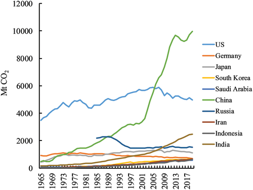
CO₂ emissions from China, the United States, India, Russia, Japan, Germany, Iran, South Korea, Indonesia, and Saudi Arabia have grown from 13,000 Mt to 23,200 Mt over the past 20 years (). China’s CO₂ emissions grew very slowly until 1978, and after China began its reform and opening up, the carbon emissions hiked rapidly from 1430 Mt to 9953 Mt. China surpassed the United States as the world’s largest contributor in CO₂ emissions in 2007 (Shao et al. Citation2016). The CO₂ emissions of the United States declined from a maximum of 5800 Mt in 2006 to nearly 5000 Mt in recent years. India, an emerging economy, has seen its CO₂ emissions growing rapidly from 170 Mt to 2480 Mt, with an average growth rate of 5.1%. Russia’s CO₂ emissions declined slowly from approximately 230 Mt in the 1990s to 140–150 Mt in the last decade. Japan’s CO₂ emissions increased from 430 Mt in 1965 to 1300 Mt in 2008, then decreased to 1200 Mt. CO₂ in Germany, reached a maximum of 1120 Mt in 1973, and then slowly declined to 680 Mt in 2019. Iran, South Korea, and Indonesia have similar trajectories of CO₂ emission changes, growing from 200 Mt to about 650 Mt. Saudi Arabia’s CO₂ emissions increased from 60 Mt in 1965 to 580 Mt in 2019. The United States, Germany, Japan, and Russia have achieved high CO₂ emissions, while CO₂ emissions in South Korea, China, Saudi Arabia, Iran, Indonesia, and India will continue to grow.

Figure 1. Trends in CO₂ emissions of major countries from 1965 to 2019 (Data source: IEA, and this study).

Figure 1. Trends in CO2 emissions of major countries from 1965 to 2019 (Data source: IEA, and this study).

Temporal change of CO₂ emissions per capita in different countries

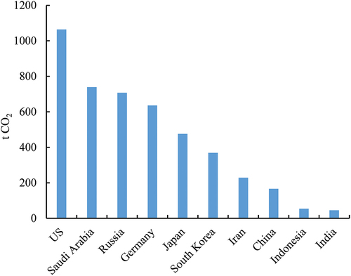
In 2019, global CO₂ emission per capita was 4.55 t CO₂ emissions per capita in high-income countries that was much higher than in middle-and low-income countries. The United States had the highest values with its CO₂ emission per capita declining from a peak of 22.5 t in 1973 to 15.1 t in 2019. Saudi Arabia has replaced the United States as the country with the highest CO₂ emissions per capita since 2011, and its value now stands at 17 t. The CO₂ emissions per capita in Germany and Japan showed a decreasing trend, with 8.2 t and 8.9 t, respectively. South Korea’s CO₂ emission per capita grew rapidly from 0.9 t to 12.3 t. CO₂ emission per capita in Russia decreased from 15 t in the 1990s to 10 t in 2019. CO₂ emissions per capita in Iran and China grew rapidly to 8 t and 7 t, respectively. Indonesia and India had lower values compared to other countries, at 2.3 t and 1.8 t in 2019. During the observation period, the cumulative CO₂ emission per capita in the United States (1064 t) was much higher than in other counties. The cumulative values of Saudi Arabia, Russia, Germany, Japan, and South Korea were 739 t, 707 t, 635 t, 476 t, and 369 t, respectively. The cumulative CO₂ emissions per capita in China, Indonesia, and India were only 168 t, 54 t, and 45 t, respectively ().

Figure 2. The cumulative CO₂ emission per capita by country from 1965 to 2019.

Figure 2. The cumulative CO2 emission per capita by country from 1965 to 2019.

Differences in driving mechanisms of CO₂ emissions from country to country

Overall changes of driving mechanisms for CO₂ emissions from country to country

The annual CO₂ emissions were calculated as the product of CI, EI, PCI, and P. Overall, the EI (−24%) and CI (−87%) effects promoted CO₂ emission reductions, while the P (+41%) and PCI (+170%) effects restrained the decrease in CO₂ emissions. The driving mechanisms differ from country to country, as shown in . The P effect had relatively small impacts in Russia and Germany, while in China, the United States, and Saudi Arabia, it brought more carbon emissions. The PCI effect boosted CO₂ emissions to different degrees in each country and was the most significant contributor in China, the United States, India, Japan, and Germany. Except for Indonesia, the CI effect had a downward impact on CO₂ emissions. The EI effect could reduce carbon emissions, but because of the high energy intensity in Iran and Saudi Arabia, it promoted an increase in the two countries.

Figure 3. Driving mechanisms of carbon emission for major countries in the world from 1965 to 2019.

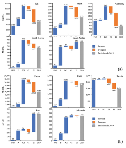
For high-income countries (), the four drivers changed as follows: (1) CO₂ emissions in the United States increased from 3840 Mt to 4965 Mt. The P (+2608 Mt) and PCI (+4813 Mt) were the most significant contributors, while the CI (−1166 Mt) and EI (−4770 Mt) had a downward influence on CO₂ emissions. (2) CO₂ emission growth in Japan was 676 Mt, to which the PCI (+1187 Mt) and P (+223 Mt) contributed significantly, and CI (−104 Mt) and EI (−630 Mt) effects had a decreasing influence on CO₂ emissions. (3) The CO₂ emissions fell by 360 Mt in Germany. The P and PCI effects contributed 56 Mt and 846 Mt CO₂ emissions, and the CI and EI effects reduced 403 Mt and 859 Mt. The P effect shifted between negative and positive and overall contributed 16% of CO₂ emissions. (4) In South Korea, CO₂ emissions increased by 613 Mt. The P and PCI effects contributed 121 Mt and 750 Mt, while the CI and EI effects reduced 120 Mt and 137 Mt. (5) CO₂ emissions increased by 584 Mt in Saudi Arabia. This was mainly driven by population growth at 411 Mt. In contrast, the contribution of PCI was 27 Mt. The CI effect was −68 Mt, while EI did not show emission reduction (+151 Mt).

The driving mechanisms of CO₂ emissions for middle-and low-income countries were also changed over years (): (1) China’s CO₂ emissions increased by 9000 Mt CO₂, to which the PCI (+15,569 Mt CO₂) and P (+1575 Mt CO₂) contributed significantly, and CI (−1446 Mt CO₂) and EI (−6233 Mt CO₂) effects reduced CO₂ emissions over the past 55 years. (2) In India, CO₂ emissions have increased by 2312 Mt over the past decades. The PCI and P contributed 2055 Mt and 719 Mt, respectively, while the CI and EI decreased by 16 Mt and 445 Mt. (3) CO₂ emissions decreased from 2172 to 1533 over the last 30 years in Russia. The P (30 Mt) and PCI (70 Mt) effects contributed little, while the CI and EI effects were −357 Mt and −482 Mt. (4) Iran’s CO₂ emissions increased by 649 Mt. Iran, as a low and middle-income country, the PCI effect only contributed 36 Mt to CO₂ emissions, much less than the P effect (+233 Mt). The CI effect contributed little to emission reduction (−69 Mt), while the EI effects even showed a positive influence (+151 Mt) due to low energy efficiency. (5) Indonesia’s CO₂ emissions change was 612 Mt. The P and PCI effects were 165 Mt and 403 Mt, while the CI and EI effects were 50 Mt and −6 Mt, respectively. The contribution of the EI effect to CO₂ emission reduction was very small (1%). As a developing country with a large population, Indonesia will continue to increase its CO₂ emissions due to population and income growth.

Temporal changes in driving mechanisms of CO₂ emissions from country to country

We analyzed the temporal changes in driving mechanisms of CO₂ emissions for these countries. As shown in , the results for high-income countries wereas follows: (1) The contribution of P and PCI to CO₂ emissions in the United States remained at 200 Mt to 300 Mt and 300 Mt to 800 Mt over most of the periods. The CI was able to partially offset CO₂ emissions (−50 Mt to −300 Mt), and the EI effectively reduced CO₂ emissions (−300 Mt to −800 Mt) since the 1970s. (2) In Japan, P and PCI effects have been decreasing year by year, from 50 Mt and 200 Mt in the 1970s to −8 Mt and 50 Mt in 2019. The trend of CI and EI effects was favorable to CO₂ emissions reductions. (3) The trend of driving mechanisms over time in Germany is similar to that of Japan. (4) In South Korea, the P effect contributed 5 Mt to 15 Mt CO₂ emissions, while the contribution of PCI ranged from 15 Mt to 110 Mt. The CI effect decreased to −12 Mt in 2015–2019, and the EI effect reduced 165 Mt CO₂ emissions since 2001. (5) The contribution of P and CI to CO₂ emissions in Saudi Arabia was slowly increasing from12 Mt and −2 Mt to 80 Mt and −20 Mt, respectively, and the PCI and EI shifted from positive to negative in promoting CO₂ emissions in 2015–2019.

Figure 4. Temporal changes in driving mechanisms of CO₂ emissions.

Figure 4. Temporal changes in driving mechanisms of CO2 emissions.

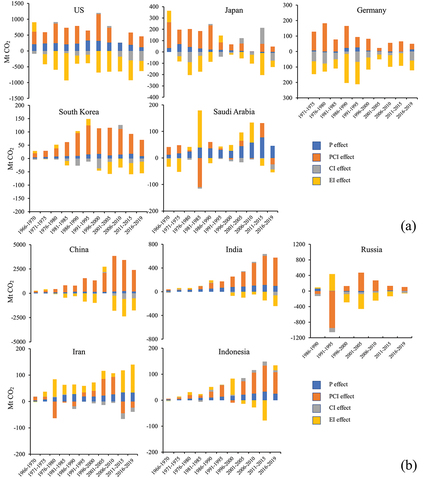
For middle-and low-income countries, the contribution of each driver to CO₂ emissions was increasing year by year, except for Russia (), as illustrated in the following: (1) In China, the contribution of P gradually increased from 72 Mt to 223 Mt and started to decrease after 2015, and the PCI contributed the most to CO₂ emissions, peaking between 2006 to 2015 (>3000 Mt), while the CI and EI contributions to CO₂ emissions reduction increased in the same period. (2) In India, the P and PCI contributions gradually increased from 20 Mt to 100 Mt and 480 Mt, respectively. The CI effect on CO₂ emissions reduction was prominent after 2015, reaching 60 Mt, and the EI effect was also increased, reaching −330 Mt reading 2011–2019. (3) In Russia, the P and PCI effects were weakening, contributing 3 Mt and 100 Mt in 2016–2019. Looking at this period in aggregate, the EI effect decreased to 45 Mt in 2016–2019, and the CI effect had the largest reduction in 1991–1996 (107 Mt). (4) In Iran, the P contributed 20 Mt – 30 Mt to CO₂ emissions, the PCI promoted emission growth (150 Mt) in 1991–2010, the CI contributed less to emission reduction, and the EI effect did not reduce CO₂ emissions. (5) In Indonesia, the contribution of P and PCI to CO₂ emissions increased from 10 Mt and 25 Mt to 25 Mt and 100 Mt, respectively, and CI and EI did not reduce CO₂ emissions.

Embodied emissions in trade and driving mechanism of CO₂ emissions at the global scale

The key variables introduced into the LMDI model in this paper included economy, population, energy intensity, and carbon intensity, and the driving mechanisms of CO₂ emissions relied on a production-based perspective. From the perspective of international trade, embodied emissions in trade are of great interest due to the geographical separation of production and consumption, which often leads to disputes over the attribution of CO₂ emissions. Therefore, we analyzed the impacts of trade on CO₂ emissions. The results showed that imports in the United States could significantly affect CO₂ emissions, with an elasticity coefficient of 0.18 (P <0.01), suggesting that the United States transferred some of its CO₂ emissions through imported products and services. The export in China, India, and Indonesia also affected their CO₂ emissions, with elasticity coefficients of 0.39 (P <0.01), 0.19 (P <0.01), and 0.58 (P <0.01), respectively. The rapid growth of CO₂ emissions in China stemmed not only from population and consumption but also from an export-oriented economy. China is known as the world’s factory, with the largest industrial manufacturing system, and at the same time, it inevitably brings the largest energy consumption and greenhouse gas emissions. The embodied emissions from developed countries to developing countries were no longer limited to industrial transfer, but also from services and products. From 2010 to 2018, embodied emissions in the services trade accounted for nearly 30% of total emissions embodied in global trade (Huo et al. Citation2021). Globally, North–North and North–South trade rose rapidly before the economic crisis in 2008, while the global chain and trade structure changed after 2008, South–South trade grew rapidly, with the resulting increase in CO₂ emissions, especially in China and India (Zhang et al. Citation2020).

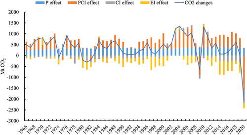
In addition, we pooled all data to analyze the driving mechanism of CO₂ emissions at the global level overtime to eliminate the impact of international trade (). The results showed that the contribution of P to CO₂ emissions increased from 230 Mt to 380 Mt. In 2020 when COVID-19 was rampant, the P effect was the only factor contributing to the increase in global emissions. The PCI effect was larger than the P effect over most periods, but it had a downward influence on CO₂ emissions in periods such as the oil crisis and the 2008 financial crisis. The CI effect reduced CO₂ emissions and has become increasingly important in emission reduction after the signing of the Paris Agreement in 2015. Many countries, such as China, have accelerated their deployment of renewable energy, and therefore the contribution of CI is increasing from −290 Mt to −616 Mt. Globally, the EI effect was the most important contributor to the emission reduction, with an average annual reduction of 196 Mt.

Figure 5. Driving mechanism of CO₂ emissions at the global level from 1965 to 2020.

Figure 5. Driving mechanism of CO2 emissions at the global level from 1965 to 2020.

Prediction of future CO₂ emissions

The regression of the STIRPAT model can well explain the relationship between CO₂ emissions and various factors in different countries, which is in line with the results of the LMDI model (). The population has a downward effect on CO₂ emissions in Japan, and the effect is close to −1%. In other countries, this factor still contributes to an increase in CO₂ emissions, with a 1% increase in population promoting 0.5%–1.2% emissions. Per capita income is the most significant factor and 1% increase can drive 0.5%–1.3% increase in CO₂ emissions. In most countries, this percentage exceeds 1%, while in Germany this value is 0.5%. In both developed and developing countries, energy intensity decrease is an important pathway to reducing CO₂ emissions. The impact of energy intensity is comparable to that of the per capita income. 1% reduction in energy intensity can bring more than 1% reduction in CO₂ emissions. However, the high energy intensity in Iran and Saudi Arabia has contributed to the increase in CO₂ emissions in both countries.

Table 2. Group regression results of STIRPAT model for sampled countries.

Download CSV Display Table

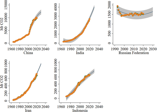
Based on the results of the STIRPAT model, we project the CO₂ emissions from the sampled countries up to 2030 under “business as usual (BAU)” to reflect the role of the driving mechanism. The CO₂ emissions show decreasing trends in the United States, Japan, and Germany, and will reach 4510 Mt, 1078 Mt, and 673 Mt, respectively (). For South Korea and Saudi Arabia, the CO₂ emissions are expected to continue to increase, reaching 755 Mt and 753 Mt, respectively, in 2030. The CO₂ emissions trends in middle and low-income countries are also different (). For Russian Federation, the CO₂ emissions will remain at around 1500 Mt. China’s CO₂ emissions will grow at a slower rate due to its improvement in energy efficiency and deployment of renewable energy. The estimation of China’s CO₂ emissions will reach a maximum of around 12,500 Mt in 2030. With the transformation of the energy mix and implementation of carbon reduction plans, China’s CO₂ emissions peak may arrive earlier than 2030. The CO₂ emissions of India, Iran, and Indonesia will continue to grow rapidly, reaching 4294, 969, and 874 Mt, respectively, in 2030.

Figure 6. The CO₂ emissions projection for high-income countries from 1960 to 2030. Green and yellow scatter denotes observation and estimation of emissions, the curve represents fitted values of estimation, and the shaded area represents the 95% confidence interval of estimation.

Figure 6. The CO2 emissions projection for high-income countries from 1960 to 2030. Green and yellow scatter denotes observation and estimation of emissions, the curve represents fitted values of estimation, and the shaded area represents the 95% confidence interval of estimation.

Figure 7. The CO₂ emissions projection for middle and low-income countries from 1960 to 2030. Green and yellow scatter denotes observation and estimation of emissions, the curve represents fitted values of estimation, and the shaded area represents the 95% confidence interval of estimation.

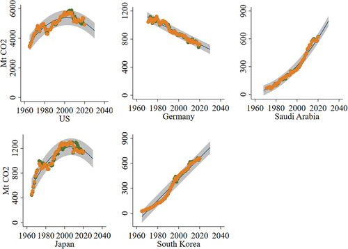
Figure 7. The CO2 emissions projection for middle and low-income countries from 1960 to 2030. Green and yellow scatter denotes observation and estimation of emissions, the curve represents fitted values of estimation, and the shaded area represents the 95% confidence interval of estimation.

The results show that countries with different economic development have very different emission trajectories. Developing countries such as China that are in transition should maintain the green and low-carbon path for economic development, improve energy efficiency to reduce the carbon intensity of industrial development, and promote low-carbon product exports. The high-income countries have higher energy efficiency and obvious “carbon leakage” effect due to the transfer of carbon-concentrated industries to other countries. As a result, CO₂ emissions in these countries show a decreasing trend in the future.

Dynamic relationships between CO₂ emission and economic development

Economic development is a major driver of increased energy consumption and CO₂ emissions. The decoupling index of CO₂ emissions and economic development in each country was calculated according to the Tapio model, as shown in . The decoupling index varied significantly in different countries over time, but no recessive coupling relationship was observed. The results show that countries with strong decoupling relationships between CO₂ emissions and economic development include the United States, Germany, Japan, and Saudi Arabia, countries with weak decoupling relationships include South Korea, China, Russia, and India, and countries with negative decoupling relationships, including Iran and Indonesia in recent years. Since CO₂ emissions are closely linked to the level of economic development, this study divided these countries into two groups: high-income and middle-income countries.

Table 3. Decoupling index of carbon emission and economic development.

Download CSV Display Table

(1) Decoupling relationships in high-income countries

The United States showed an expansive negative decoupling relationship from 1965 to 1970, and since then, the relationship has shifted between a weak decoupling and a strong decoupling. After 2006, this relationship showed a strong decoupling relationship. During the observation period, Germany showed a weak decoupling relationship in 1965–1970 and 1981–1985, and a strong decoupling relationship in the rest of the period, indicating that economic development decoupled from carbon emissions since 1986. The relationship between the economy and emissions in Japan evolved from decoupling in the 1970s to expansive coupling in the 1980s. It changed from expansive negative decoupling to weak decoupling in the 1990s and evolved from expansive negative decoupling to recessive decoupling in the 21st century. Japan decoupled economic development from carbon emissions in 2011. For most of the period until 1995, the growth of carbon emissions in South Korea exceeded the growth in the economy. Since then, the relationship showed a weak decoupling relationship, except for the period 2006–2010 (expansive coupling). South Korea did not have a decoupling relationship. Saudi Arabia’s economy is an oil-based economy that includes energy-intensive industrial, construction, and transportation sectors. As a result, Saudi Arabia’s carbon emissions and economic development mainly exhibited a coupling relationship until 2016 and a strong decoupling relationship during 2016–2019.

(2) Decoupling relationships in middle-and low-income countries

China has not shown a decoupling relationship between CO₂ emissions and economic development for a long time. In the period 1965–1975, carbon emissions grew faster than economic development, showing a coupling relationship. Since China’s reform and opening-up, the CO₂ emissions and economic development showed an expansive negative decoupling relationship, except for the period 2001–2005 with a weak decoupling relationship. Russia showed a strong decoupling relationship from 2000 to 2015, while this relationship shifted to weak decoupling in 2016. During 1965–2010, Iran’s CO₂ emission growth was higher than economic growth, and the relationship mainly showed expansive coupling and expansive negative decoupling. Iran’s economy declined severely, and the economic development pattern shifted to the worst one, with economic recession but increasing CO₂ emissions, showing a strong negative decoupling. Indonesia’s economic development and CO₂ emissions evolved from weak decoupling to expansive coupling and weak decoupling from 1965 to 2015, whereas during 2016–2019, this relationship shifted to a coupling relationship. During the observation period, the CO₂ emissions and economic development in India mainly showed an expansive negative decoupling and expansive coupling relationship, while showing a weak decoupling relationship in 1965–1970, 1996–2000, and 2016–2019.

Drivers affecting relationships between emissions and economy

We use the combined model (LMDI and Tapio model) to further analyze the impacts of the four drivers on dynamic relationships between economic development and CO₂ emissions. The decoupling elasticity coefficients reflect the drivers facilitating (negative values) or inhibiting (positive values) this decoupling relationship. The population is not conducive to the decoupling relationship between CO₂ emissions and economic development, especially for Saudi Arabia, Iran, India, Indonesia, and the United States. This driver has the strongest inhibitory effect in Saudi Arabia, and the decoupling elasticity coefficient is around 4 in recent years. The inhibitory effects of population in China, the Russian Federation, Japan, and South Korea are limited over the past decade, and their decoupling elasticity coefficients are less than 0.3. Per capita income is also a driver of coupling relationships between economic development and CO₂ emissions in the sampled countries, and the decoupling elasticity coefficient is in the range of 1–4. The results indicate that population is no longer a hindrance to the decoupling of CO₂ emissions and economic development, but per capita income (affluence) is the major detrimental factor for decoupling.

The drivers that facilitate the decoupling include carbon intensity and energy intensity over most of the period for most countries. Carbon intensity in Germany, the United States, and Japan played significant roles in promoting decoupling and their decoupling elasticity coefficients are −2.0, −1.1, and −2.2, respectively. The role of carbon intensity in China, South Korea, the Russian Federation, and Saudi Arabia is increasing year by year, and their decoupling elasticity of carbon intensity approaching −1. The decoupling effect of energy intensity was significant in Germany, Japan, Russia, the United States, and China, and their decoupling elasticity coefficients exceed −2. While the energy intensity in India, South Korea, and Indonesia showed limited effects of promoting decoupling recently. In Iran and Saudi Arabia, it shifted between positive and negative effects on decoupling over the past decades.

Conclusion and discussion

This study constructed an equation including population (P), income (PCI), carbon intensity (CI), and energy intensity (EI) variables, and explored driving mechanisms at the country level for China, the United States, India, Russia, Japan, Germany, Iran, South Korea, Indonesia, and Saudi Arabia and the global level based on the LMDI model. The analysis showed that P and PCI were increasing at different rates and promoting CO₂ emissions increase and CI and EI are decreasing at different levels and conductive to CO₂ emissions increase, and these four factors together influenced the trend of CO₂ emissions. Countries with larger contributions of P effect to CO₂ emissions included the United States (+2608 Mt) and China (+1574 Mt). The contribution of the PCI effect was larger in China (+15,569 Mt), the United States (+4812 Mt), India (+2056 Mt), and Japan (+1187 Mt). Countries that reduced more CO₂ emissions due to decreasing carbon intensity included China (−1446 Mt), the United States (−1166 Mt), Germany (−402 Mt), and Russia (−357 Mt). Energy intensity decrease was the most significant factor to reduce CO₂ emission, especially in China (−6360 Mt), the United States (−4770 Mt), Germany (−859 Mt), and Japan (−630 Mt). Globally, economic growth and population change drove the increase in CO₂ emissions, while decreasing intensity effects reduce them. The analysis quantifies the driving mechanisms of CO₂ emissions and compares the patterns of population, economic, and CO₂ emissions changes, and these findings are expected to provide insight for China and other countries to address climate change.

The analysis of driving mechanisms for CO₂ emissions on both the global and country levels showed that intensity reduction was the main pathway to reducing CO₂ emissions. Carbon intensity decrease was mainly accomplished by deploying renewable energy to replace the fossil energy. Renewable energy capacity reached 2799 GW in 2020, up 10.3% from 2019. More than 260 GW of renewable energy installed in 2020, with China accounting for more than 50% (136 GW) according to World Energy Outlook 2021. This was closely related to the governments that have developed policies to reduce CO₂ emissions. At the same time, some countries (e.g., Russia) stopped using fossil fuels to generate electricity, which also supported the growth of renewable energy. Energy intensity reduction means energy efficiency improvement. Therefore, for developed countries with higher energy efficiency, improving energy structure and promoting renewable energy substitution are the main paths for emission reduction, while for developing countries, improving energy efficiency is an effective way to reduce CO₂ emissions. In addition to the energy transition, energy efficiency improvement, and application of technologies, for export-oriented economies like China, promoting industrial transformation and reducing the export of energy-intensive products and services are also important ways of reducing emissions. Moreover, CO₂ emissions trading system (ETS) is also an important economic instrument, such as ETS in Europe Union, Regional Greenhouse Gas Initiative in the United States, and the Carbon Market in China.

A comparison of CO₂ emissions trends in different countries showed that countries such as the United States, Japan, and Germany have already experienced phase peaks and these peaks generally occur when energy intensities are below 0.4 kg CO₂/USD. Decoupling analysis showed that developed countries such as the United States, Germany, and Japan achieved decoupling in the last decade while developing countries such as China and India showed weak decoupling relationships. Governments should reduce the carbon intensity and encourage technological innovation to achieve a decoupling relationship between CO₂ emissions and economic development. Policymakers should encourage the public to change their lifestyles, such as rational consumption and green travel to reduce carbon footprint, especially in developed countries, where CO₂ emissions per capita are much higher than those in developing countries. The average and cumulative CO₂ emissions per capita in the United State over the past 55 years have reached 19.3 t and 1063 tons.

In addition to the variables introduced into the model and international trade, other potential factors also affect CO₂ emissions, including climate policy, renewable energy, investment, etc. The Climate Change Performance Index (CCPI) incorporates these factors. The CCPI is an independent monitoring tool for tracking countries’ climate protection performance based on four categories: greenhouse gas (GHG) emissions, renewable energy, energy use, and climate policy, and another similar tool is the African Climate Change Policy Performance Index (ACCPI) (Burck et al. Citation2021; Epule et al. Citation2021). The CCPI 2022 was issued by Germanwatech, New Climate Institute, and Climate Action Network International in 2021. The report noted that India, Germany, and Indonesia had good performances, ranking 10^th, 13^th, and 27^th respectively. China fell five places to 38^th in this year’s CCPI, but with mixed ratings across categories. China’s climate policy performance was “high,” while its GHG emissions and energy use were rated as “very low,” and “medium” for renewable energy. Japan retained its rank of 45^th. The United States, Russia, South Korea, Iran, and Saudi Arabia received “very low” ratings (Burck et al. Citation2021).

Climate policy is important for countries to achieve emission targets or intensity indicators, involving social, economic, and energy development aspects. For emerging economies pursuing high economic growth, absolute emission targets should take precedence over intensity targets to reduce CO₂ emissions. Renewable energy was discussed above as one of the measures for emission reduction. The development and deployment of renewable energy, combined with circular economy patterns, can contribute to the sustainable development of emerging economies. Investment is one of the factors that stimulate CO₂ emissions. In the case of China, for example, investment and capital accumulation were important factors in the sectoral shift to a carbon-intensive economic structure between 2002 and 2009 (Guan et al. Citation2014). These factors could not be included in one paper, but will be further studied in the future. Moreover, due to the lack of industry data for each country, this study did not analyze the relationship between industrial carbon emissions and economic development in different countries. Therefore, the driving mechanism study, as well as decoupling analysis, could be updated with more detailed data. Furthermore, suitable scenario projections need to be explored in the future to simulate the compliance of these countries to the Paris Agreement.

Supplemental material

Supplemental Material

Download MS Word (15.7 KB)

Acknowledgments

This work was supported by the National Natural Science Foundation of China (Grant No. 71761147001, No. 42030707), the National Key R & D Program of China (2019YFC0507505), the International Partnership Program by the Chinese Academy of Sciences (121311KYSB20190029), and the Fundamental Research Fund for the Central Universities (No.20720210083).

Disclosure statement

No potential conflict of interest was reported by the author(s).

Data availability statement

The data that supports the findings of this study are available from the corresponding author, Lu, Y. L., upon reasonable request.

Supplementary material

Supplemental data for this article can be accessed here

Correction Statement

This article has been corrected with minor changes. These changes do not impact the academic content of the article.

Additional information

Funding

This work was supported by the National Natural Science Foundation of China [71761147001, 42030707]; National Key Research and Development Program of China [2019YFC0507505]; Fundamental Research Fund for the Central Universities [20720210083]; International Partnership Program by the Chinese Academy of Sciences [121311KYSB20190029].

References

Ahmed, M., and M. Azam. 2016. “Causal Nexus between Energy Consumption and Economic Growth for High, Middle and Low Income Countries Using Frequency Domain Analysis.” Renewable and Sustainable Energy Reviews 60: 1–14. doi:10.1016/j.rser.2015.12.174.
Web of Science ®Google Scholar
Alkhathlan, K., and M. Javid. 2013. “Energy Consumption, Carbon Emissions and Economic Growth in Saudi Arabia: An Aggregate and Disaggregate Analysis.” Energy Policy 62: 1525–1532. doi:10.1016/j.enpol.2013.07.068.
Web of Science ®Google Scholar
Ang, B. W. 2015. “LMDI Decomposition Approach: A Guide for Implementation.” Energy Policy 86: 233–238. doi:10.1016/j.enpol.2015.07.007.
Web of Science ®Google Scholar
Arouri, M. E. H., A. Ben Youssef, H. M’Henni, and C. Rault. 2012. “Energy Consumption, Economic Growth and CO2 Emissions in Middle East and North African Countries.” Energy Policy 45: 342–349. doi:10.1016/j.enpol.2012.02.042.
Web of Science ®Google Scholar
Balezentis, T. 2020. “Shrinking Ageing Population and Other Drivers of Energy Consumption and CO2 Emission in the Residential Sector: A Case from Eastern Europe.” Energy Policy 140: 111433. doi:10.1016/j.enpol.2020.111433.
Web of Science ®Google Scholar
Begum, R. A., K. Sohag, S. M. S. Abdullah, and M. Jaafar. 2015. “CO2 Emissions, Energy Consumption, Economic and Population Growth in Malaysia.” Renewable and Sustainable Energy Reviews 41: 594–601. doi:10.1016/j.rser.2014.07.205.
Web of Science ®Google Scholar
Burck, J., T. Uhlich, C. Bals, N. Höhne, L. Nascimento, J. Wong, A. Tamblyn, and J. Reuther. 2021. “Climate Change Performance Index.” 2022.
Google Scholar
Dietz, T., K. A. Frank, C. T. Whitley, J. Kelly, and R. Kelly. 2015. “Political Influences on Greenhouse Gas Emissions from US States.” Proceedings of the National Academy of Sciences 112 (27): 8254–8259. doi:10.1073/pnas.1417806112.
PubMed Web of Science ®Google Scholar
Epule, T. E., A. Chehbouni, D. Dhiba, M. W. Moto, and C. Peng. 2021. “African Climate Change Policy Performance Index.” Environmental and Sustainability Indicators 12: 100163. doi:10.1016/j.indic.2021.100163.
Google Scholar
Grubler, A., C. Wilson, N. Bento, B. Boza-Kiss, V. Krey, D. L. McCollum, N. D. Rao, et al. 2018. “A Low Energy Demand Scenario for Meeting the 1.5 °C Target and Sustainable Development Goals without Negative Emission Technologies.” Nature Energy 3 (6): 515–527. doi:10.1038/s41560-018-0172-6.
Web of Science ®Google Scholar
Guan, D., S. Klasen, K. Hubacek, K. Feng, Z. Liu, K. He, Y. Geng, and Q. Zhang. 2014. “Determinants of Stagnating Carbon Intensity in China.” Nature Climate Change 4 (11): 1017–1023. doi:10.1038/nclimate2388.
Web of Science ®Google Scholar
Huo, J., J. Meng, Z. Zhang, Y. Gao, H. Zheng, D. M. Coffman, J. Xue, Y. Li, and D. Guan. 2021. “Drivers of Fluctuating Embodied Carbon Emissions in International Services Trade.” One Earth 4 (9): 1322–1332. doi:10.1016/j.oneear.2021.08.011.
Google Scholar
Jorgenson, A. K. 2014. “Economic Development and the Carbon Intensity of Human Well-being.” Nature Climate Change 4 (3): 186–189. doi:10.1038/nclimate2110.
Web of Science ®Google Scholar
Kraft, J., and A. Kraft. 1978. “On the Relationship between Energy and GNP.” Journal of Energy and Development 3: 401–403.
Google Scholar
Levin, A., C. F. Lin, and C. S. James Chu. 2002. “Unit Root Tests in Panel Data: Asymptotic and Finite-sample Properties.” Journal of Econometrics 108 (1): 1–24. doi:10.1016/S0304-4076(01)00098-7.
Web of Science ®Google Scholar
Li, M. J., and W. Q. Tao. 2017. “Review of Methodologies and Polices for Evaluation of Energy Efficiency in High Energy-consuming Industry.” Applied Energy 187: 203–215. doi:10.1016/j.apenergy.2016.11.039.
Web of Science ®Google Scholar
Liddle, B. 2015. “What are the Carbon Emissions Elasticities for Income and Population? Bridging STIRPAT and EKC via Robust Heterogeneous Panel Estimates.” Global Environmental Change 31: 62–73. doi:10.1016/j.gloenvcha.2014.10.016.
Web of Science ®Google Scholar
Liu, W., W. J. McKibbin, A. C. Morris, and P. J. Wilcoxen. 2020. “Global Economic and Environmental Outcomes of the Paris Agreement.” Energy Economics 90: 104838. doi:10.1016/j.eneco.2020.104838.
Web of Science ®Google Scholar
Lu, Y., Y. Zhang, X. Cao, C. Wang, Y. Wang, M. Zhang, R. C. Ferrier, et al. 2019. “Forty Years of Reform and Opening Up: China’s Progress toward a Sustainable Path.” Science Advances 5 (8). doi:10.1126/sciadv.aau9413.
Web of Science ®Google Scholar
Mardani, A., E. K. Zavadskas, D. Streimikiene, A. Jusoh, and M. Khoshnoudi. 2017. “A Comprehensive Review of Data Envelopment Analysis (DEA) Approach in Energy Efficiency.” Renewable and Sustainable Energy Reviews 70: 1298–1322. doi:10.1016/j.rser.2016.12.030.
Web of Science ®Google Scholar
Peters, G. P., R. M. Andrew, J. G. Canadell, P. Friedlingstein, R. B. Jackson, J. I. Korsbakken, C. Le Quéré, and A. Peregon. 2020. “Carbon Dioxide Emissions Continue to Grow Amidst Slowly Emerging Climate Policies.” Nature Climate Change 10 (1): 3–6. doi:10.1038/s41558-019-0659-6.
Web of Science ®Google Scholar
Pompermayer Sesso, P., S. F. Amâncio Vieira, I. D. Zapparoli, and U. A. Sesso Filho. 2020. “Structural Decomposition of Variations of Carbon Dioxide Emissions for the United States, the European Union and BRIC.” Journal of Cleaner Production 252: 119761. doi:10.1016/j.jclepro.2019.119761.
Web of Science ®Google Scholar
Robalino López, A., Á. Mena Nieto, J. E. García Ramos, and A. A. Golpe. 2015. “Studying the Relationship between Economic Growth, CO2 Emissions, and the Environmental Kuznets Curve in Venezuela (1980–2025).” Renewable and Sustainable Energy Reviews 41: 602–614. doi:10.1016/j.rser.2014.08.081.
Web of Science ®Google Scholar
Shao, S., J. Liu, Y. Geng, Z. Miao, and Y. Yang. 2016. “Uncovering Driving Factors of Carbon Emissions from China’s Mining Sector.” Applied Energy 166: 220–238. doi:10.1016/j.apenergy.2016.01.047.
Web of Science ®Google Scholar
Sharif Hossain, M. 2011. “Panel Estimation for CO2 Emissions, Energy Consumption, Economic Growth, Trade Openness and Urbanization of Newly Industrialized Countries.” Energy Policy 39 (11): 6991–6999. doi:10.1016/j.enpol.2011.07.042.
Web of Science ®Google Scholar
Shuai, C., L. Shen, L. Jiao, Y. Wu, and Y. Tan. 2017. “Identifying Key Impact Factors on Carbon Emission: Evidences from Panel and Time-series Data of 125 Countries from 1990 to 2011.” Applied Energy 187: 310–325. doi:10.1016/j.apenergy.2016.11.029.
Web of Science ®Google Scholar
Tapio, P. 2005. “Towards a Theory of Decoupling: Degrees of Decoupling in the EU and the Case of Road Traffic in Finland between 1970 and 2001.” Transport Policy 12 (2): 137–151. doi:10.1016/j.tranpol.2005.01.001.
Web of Science ®Google Scholar
Tong, D., Q. Zhang, Y. Zheng, K. Caldeira, C. Shearer, C. Hong, Y. Qin, and S. J. Davis. 2019. “Committed Emissions from Existing Energy Infrastructure Jeopardize 1.5 °C Climate Target.” Nature 572 (7769): 373–377. doi:10.1038/s41586-019-1364-3.
PubMed Web of Science ®Google Scholar
Vélez Henao, J.-A., D. Font Vivanco, and J.-A. Hernández Riveros. 2019. “Technological Change and the Rebound Effect in the STIRPAT Model: A Critical View.” Energy Policy 129: 1372–1381. doi:10.1016/j.enpol.2019.03.044.
Web of Science ®Google Scholar
Wang, C., F. Wang, X. Zhang, Y. Yang, Y. Su, Y. Ye, and H. Zhang. 2017. “Examining the Driving Factors of Energy Related Carbon Emissions Using the Extended STIRPAT Model Based on IPAT Identity in Xinjiang.” Renewable and Sustainable Energy Reviews 67: 51–61. doi:10.1016/j.rser.2016.09.006.
Web of Science ®Google Scholar
Wang, Q., R. Jiang, and L. Zhan. 2019. “Is Decoupling Economic Growth from Fuel Consumption Possible in Developing Countries? – A Comparison of China and India.” Journal of Cleaner Production 229: 806–817. doi:10.1016/j.jclepro.2019.04.403.
Web of Science ®Google Scholar
Wang, S., C. Fang, X. Guan, B. Pang, and H. Ma. 2014. “Urbanisation, Energy Consumption, and Carbon Dioxide Emissions in China: A Panel Data Analysis of China’s Provinces.” Applied Energy 136: 738–749. doi:10.1016/j.apenergy.2014.09.059.
Web of Science ®Google Scholar
Wiebe, K., H. Lotze Campen, R. Sands, A. Tabeau, D. van der Mensbrugghe, A. Biewald, B. Bodirsky, et al. 2015. “Climate Change Impacts on Agriculture in 2050 under a Range of Plausible Socioeconomic and Emissions Scenarios.” Environmental Research Letters 10 (8): 085010. doi:10.1088/1748-9326/10/8/085010.
Web of Science ®Google Scholar
York, R., E. A. Rosa, and T. Dietz. 2003. “STIRPAT, IPAT and ImPACT: Analytic Tools for Unpacking the Driving Forces of Environmental Impacts.” Ecological Economics 46 (3): 351–365. doi:10.1016/S0921-8009(03)00188-5.
Web of Science ®Google Scholar
Zhang, Z., D. Guan, R. Wang, J. Meng, H. Zheng, K. Zhu, and H. Du. 2020. “Embodied Carbon Emissions in the Supply Chains of Multinational Enterprises.” Nature Climate Change 10 (12): 1096–1101. doi:10.1038/s41558-020-0895-9.
Web of Science ®Google Scholar
Zheng, X., Y. Lu, J. Yuan, Y. Baninla, S. Zhang, N. C. Stenseth, D. O. Hessen, H. Tian, M. Obersteiner, and D. Chen. 2020. “Drivers of Change in China’s Energy-related CO 2 Emissions.” Proceedings of the National Academy of Sciences 117 (1): 29–36. doi:10.1073/pnas.1908513117.
PubMed Web of Science ®Google Scholar
Zhou, Y., and Y. Liu. 2016. “Does Population Have a Larger Impact on Carbon Dioxide Emissions than Income? Evidence from a Cross-regional Panel Analysis in China.” Applied Energy 180: 800–809. doi:10.1016/j.apenergy.2016.08.035.
Web of Science ®Google Scholar

Driving mechanisms for decoupling CO₂ emissions from economic development in the ten largest emission countries

ABSTRACT

Introduction