Spatial patterns and influencing factors of intraurban particulate matter in the heating season based on taxi monitoring

ABSTRACT

Urbanization has introduced a series of environmental problems worldwide, and particulate matter (PM) is one of the main threats to human health. Due to the lack of high-resolution, large-scale monitoring data, few studies have analyzed the intraurban spatial distribution pattern of PM at a fine scale. In this study, portable air monitors carried by five taxis were used to collect the concentrations of PM₁, PM_2.5 and PM₁₀ for five months in Shenyang during the heating season. The results showed that high concentrations of PM were distributed in the suburbs, while relatively low concentration areas were found in the central area. Agricultural, industrial and development zones had higher concentration values among the eight observed types. The PM concentration exhibited strong spatial autocorrelation based on Moran’s I index analysis. Meteorological factors were the most important influencing factors of the three pollutants, and their total contribution rate accounted for more than 80% among the 13 factors according to boosted regression trees analysis. The taxi monitoring method we proposed was a more efficient and feasible method for monitoring urban air pollution and could obtain higher spatial-temporal resolution data at a lower cost to elucidate the region’s dynamic air pollution distribution patterns.

KEYWORDS:

• Particulate matter
• taxi monitoring
• heating season
• spatial pattern
• urbanization
• Shenyang

Introduction

With the rapid progress of urbanization in China, a series of environmental hazards have been induced, such as environmental deterioration, urban heat island induction, and population expansion (Zhao, Zhang, and Destech Publicat 2016). A serious issue is air pollution caused by rising resource utilization and energy consumption, which will affect the quality of life and health of urban residents (Kwag et al. 2021; Liu et al. 2016, 2020; Shi et al. 2018; Yang et al. 2022). Particle matter (PM) pollution resulting from fossil fuel combustion is particularly serious in China, especially in heavy industrial and northern heating cities (Huang, Yan, and Zhang 2018). China has implemented a series of policies to alleviate air pollution in recent years, such as the “Air Pollution Prevention and Control Action Plan” in 2013 and the “Three-year Plan on Defending the Blue Sky” in 2018 (Fan, Zhao, and Yang 2020; Zeng et al. 2019). As a result, the national annual mean PM_2.5 was reduced by 32% during 2013–2017, which led to a 14% reduction in premature deaths due to long-term exposure (Xue et al. 2019). However, the air pollutant concentrations throughout China are still higher than the World Health Organization guidelines, and urban haze episodes are still the major threats to human health and the environment (Filonchyk and Yan 2018; Zeng et al. 2019). In China, the region with PM_2.5 concentrations greater than 35 μg/m³ still accounted for 19.73% in 2020 (Song et al. 2022). It is well known that long-term exposure to PM is harmful to public health, especially that of particles less than 10 μm in diameter, which could cause more serious problems because they can penetrate the lungs and some can even enter blood (Baccarelli et al. 2011; Guo et al. 2021; Ho et al. 2015; Shahpoury et al. 2021; Wang et al. 2020). Compared with PM_2.5 and PM₁₀, PM₁ can be inhaled deeper into human lungs and contains toxins produced by combustion. At the same time, PM also promotes harm to the environment, such as low visibility, which affects daily travel safety (Li et al. 2022; Wan et al. 2020). Research on PM has recently become a topic of major interest and has been carried out on various spatial scales.

Currently, research on atmospheric PM mainly focuses on three spatial scales. At the macroscale of countries or urban agglomerations, previous researchers have studied the regional distribution of PM through fixed monitoring sites, pollutant emission inventories or satellite remote sensing. The pollutant patterns in Chinese cities show that the PM_2.5 concentration is higher to the east of the Hu Line and lower to the west (Song et al. 2022). The highest concentration of PM_2.5 is located in the central and eastern regions and Tarim Basin in Xinjiang (He et al. 2022; Song et al. 2022). Clark, Millet, and Marshall (2011) analyzed the relationships between the climate, urban layout and air quality based on stepwise linear regression for multiple urban areas in 111 American cities using data from monitoring stations. The results indicated that population density and centrality have an important impact on the concentration of PM, and the spatial distribution of the population and meteorological factors have basically the same contribution rate to PM concentrations (Clark, Millet, and Marshall 2011). At the mesoscale of administrative regions, many researchers have studied the distribution and influencing factors of particulate concentrations in cities by establishing land use regression (LUR) models. According to the specific conditions of various regions, the predictive variables selected by the model were concentrated in several aspects, such as transportation, land use, and physical geography, with less consideration for meteorological elements (Briggs et al. 1997; Hoek et al. 2008). Lee et al. (2017) conducted a study on air pollution in Hong Kong, China, with a high density of human settlements through the LUR model and found that the PM_2.5 concentration was high in the northwest due to transport from mainland China (Lee et al. 2017). At the microscale of urban blocks, atmospheric environment research is mainly based on mobile monitoring data and computational fluid dynamics (CFD) model simulations. Liu et al. (2020) conducted field surveys at a university campus in Wuhan to analyze the temporal and spatial variations in traffic-related PM. The results indicated that traffic emissions may account for 50% of the measured campus pollution. The impact range of PM_1.0 and PM_2.5 was 1.5 times that of PM₁₀. The influence of traffic emissions on PM_1.0 was negatively correlated with the atmospheric background concentration (Liu et al. 2020).

However, in addition to the above three spatial scales, there is a fourth spatial scale: intraurban. The urban interior is a highly complex system consisting of population, material and energy exchanges, and the spatial difference in the PM concentration within cities is much greater than that between cities (Miller et al. 2007). With the development of science and technology, satellite-retrieved AOD products have been used to estimate the urban-scale PM_2.5 concentration, which can better reflect the overall concentration distribution within cities (Chen et al. 2020). However, the spatial resolution of AOD data is still inadequate at the intraurban and block scales. Additionally, most satellite-retrieved AOD-PM_2.5 concentrations are constrained by weather conditions and cloud ages (Fu, Kelly, and Clinch 2020). There are few national atmospheric monitoring stations in a city, and their locations are fixed. It should be noted that scientists could monitor the representative area, which ranges from 0.25 to 16.25 km² of a single station of PM_2.5, by using 169 fixed monitoring stations, and the accuracy of this method depends on the origin and source of aerosol (Shi et al. 2018; Zhao et al. 2019). Although some cities in China have some dense networks of low-cost sensors for PM observations since 2015 (Shi et al. 2018; Zhao et al. 2019), due to the lack of publicly available high-spatial resolution data on fine particle concentrations, research on the distribution characteristics of PM in interior cities is insufficient. Taxi-based mobile monitoring could obtain PM data on a fine scale and has promising prospects for exploring the spatial patterns of PM pollution in inner cities.

Most northern cities in China suffer from severe atmospheric particulate pollution, especially in urban industrial areas. Due to the dense population and many pollution sources, air pollution is particularly serious during the heating period (Bai et al. 2019; Fu, Kelly, and Clinch 2020; Mardones and Sanhueza 2015; Zhang et al. 2020). The heating season is the most severe period of air pollution in Shenyang, which is prone to continuous heavy pollution weather, and sometimes the maximum concentration of PM_2.5 exceeds 1,000 μg/m³. In the 2019 national air quality report, Shenyang ranked in the last 20 in the comprehensive index evaluation of the ambient air quality of 168 cities in China. Haze and other weather phenomena seriously affect the quality of the living environment for residents, and this has become an important factor restricting the development of Shenyang City.

In this study, taxi-based monitoring, as a mobile monitoring method that can carry out long-operation intervals and large-scale fine monitoring (Messier et al. 2018), was used to monitor the PM concentration in Shenyang during the heating season. Our aims were to explore 1) the spatial distribution characteristics and spatial autocorrelation of PM in the urban area of Shenyang and 2) the contribution rate and marginal effects of influencing factors on the distribution of PM in the urban area of Shenyang during the heating season. It was expected that the analysis of the PM distribution pattern in the heating season of northern cities could provide effective direction for industrial restructuring, green space optimization and transportation planning in the future.

Materials and methods

Study area

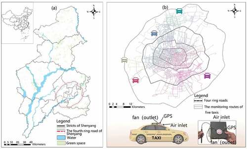
The urban area of Shenyang city, which is the capital of Liaoning Province, was chosen as our study area. It is an important central city and acts as an advanced equipment manufacturing base in Northeast China. Shenyang is a heavy industrial city, and fossil fuel combustion is the main source of heating energy during the heating season, which results in serious air pollution in winter (Li et al. 2020). There are 11 national fixed monitoring stations in the city. The data monitored by each station include the AQI and the PM, SO₂, NO₂, O₃, CO concentrations, etc. In this study, the urban area refers to the region within the fourth ring road, which covers an area of 1227.68 km² and contained more than 6 million people in 2019 (Figure 1(a)).

Figure 1. Location of the study area (a) and monitoring routes (b).

Taxi monitoring

A Sniffer4D device with a PM sensor was used to collect PM₁, PM_2.5 and PM₁₀ at a height of 1.5 m. This device has a sensor that can simultaneously collect PM and meteorological data (temperature and relative humidity), is suitable for mobile monitoring and can be installed on unmanned aerial vehicles or cars (Li et al. 2020). The PM sensor is a miniaturized laser photometer based on the light scattering principle. The time resolution of the monitoring sensor was 1 s, and the accuracy of the PM measurements was 1 μg/m³. The ambient temperature with a resolution of 0.1°C and the relative humidity with a resolution of 0.1% were measured by a meteorological sensor.

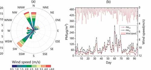
Five taxis-carrying monitors (Sniffer 4D) were used as mobile monitoring systems to collect PM concentrations in the Shenyang urban area. The monitoring period was five months long from 1 November 2019, to 31 March 2020, which covers the whole heating season in Shenyang. Due to the interference of the Spring Festival holidays during the monitoring period, the number of days with valid data was 95 days. The five taxis came from different districts, so the monitoring covered most of the study area (Figure 1(b)). According to the climate data of the Shenyang area of the National Climate Data Center (http://data.cma.cn/), the dominant wind direction during the monitoring period was northwest and southwest (Figure 2(a)). The average PM concentrations during this period were obtained from the online air quality monitoring platform of the national monitoring stations (https://www.aqistudy.cn). According to the air quality index (AQI), the air quality was divided into six levels ranging from good to poor: excellent quality, good quality, slight pollution, moderate pollution, heavy pollution and serious pollution (MEP 2012). Ten days during the monitoring period reported a pollution level higher than that of moderate pollution (Figure 2(b)).

Figure 2. Wind rose (a) and the average particulate matter concentrations (b) in Shenyang during the monitoring period.

Data processing

The concentration data collected by taxi monitoring need to be processed before analysis. To eliminate outliers, the original data with residuals larger than three times the standard deviation of the residuals were identified as anomalous data and eliminated (Sajani et al. 2018). The temporal variation in the PM daily concentration was mainly caused by changes in the meteorological conditions, and the variation in emissions also has certain contributions (de Hartog et al. 2005; Demuzere et al. 2009). Therefore, the monitoring concentration of the 11 national monitoring stations (R₁-R₁₁) of each monitoring day (i) in Shenyang was used as the reference to normalize the measured PM values collected during the 95 days of monitoring (Equation 1(1) $\begin{array}{rl}& C\left(X\right)=\frac{1}{11}\times \left[\left(\frac{\sqrt[95]{{\prod }_{i=1}^{95}{C}_{i\left(R1\right)}}}{C_{i\left(R1\right)}}\right)\right.\\ & +\left(\frac{\sqrt[95]{{\prod }_{i=1}^{95}{C}_{i\left(R2\right)}}}{C_{i\left(R2\right)}}\right)+\cdots \\ & \left.+\left(\frac{\sqrt[95]{{\prod }_{i=1}^{95}{C}_{i\left(R11\right)}}}{C_{i\left(R11\right)}}\right)\right]\times C{\left(x\right)}_i\end{array}$(1) ) (Merbitz, Fritz, and Schneider 2012).

(1) $\begin{array}{rl}& C\left(X\right)=\frac{1}{11}\times \left[\left(\frac{\sqrt[95]{{\prod }_{i=1}^{95}{C}_{i\left(R1\right)}}}{C_{i\left(R1\right)}}\right)\right.\\ & +\left(\frac{\sqrt[95]{{\prod }_{i=1}^{95}{C}_{i\left(R2\right)}}}{C_{i\left(R2\right)}}\right)+\cdots \\ & \left.+\left(\frac{\sqrt[95]{{\prod }_{i=1}^{95}{C}_{i\left(R11\right)}}}{C_{i\left(R11\right)}}\right)\right]\times C{\left(x\right)}_i\end{array}$(1)

where C(X) is the normalized PM value (μg/m³); R₁-R₁₁ are the 11 national monitoring stations; j is the monitoring day; C_i(R1) is the PM concentration of national monitoring Station R₁ on monitoring Day i; and C(x)_i is the measured PM concentration by taxi on monitoring Day i (μg/m³). By normalizing the PMs in the long time series to the same background value, the hot and cold spot areas of the PMs could be obtained.

We multiplied the C(X) produced by the monitoring data to obtain the normalized data for each day. Since most urban blocks in Shenyang cover an area of approximately 500 × 500 m, we divided the study area into a 500 × 500 m grid space that consisted of 2570 cells. We calculated the average concentration of PM for each grid cell. We used fishnets to analyze the spatial distribution pattern and spatial autocorrelation of atmospheric PM.

Spatial autocorrelation analysis

Global Moran’s I and local Moran’s I were applied to examine the spatial correlation of the three PM groups based on the normalized data of 500 × 500 m grids. The values of global Moran’s I range from −1 to 1. A global Moran’s I close to 1 or −1 indicates an aggregation distribution, and a value close to 0 represents a random distribution (Chen, Yue, and La Rosa 2020). Then, we used local Moran’s I to visualize the aggregation or dispersion pattern of PMs. A high positive Moran’s I value implied that the air pollutants were spatially clustered, and the spatial cluster types include high-high clusters (HH, high PM concentrations in a high PM concentration neighborhood) and low-low clusters (LL, low PM concentrations in a low PM concentration neighborhood). Additionally, a high negative Moran’s I value implies that the air pollutant values were different from the surrounding zones and include high-low outliers (HL, high PM concentrations in a low PM concentration neighborhood) and low-high outliers (LH, low PM concentrations in a high PM concentration neighborhood).

Boosted regression trees

There are many factors that affect the concentration and distribution pattern of PM, and most research results have indicated that the PM_2.5 concentration is positively correlated with surface solar radiation, temperature, relative humidity, particle size ratio, aerosol optical depth (AOD), and cultivated land cover and negatively correlated with air pressure, precipitation, wind speed, and forest coverage (Chen et al. 2020; Fu, Kelly, and Clinch 2020; Stowell et al. 2020). In general, it is difficult to distinguish the contribution of a single influencing factor to the measured pollutant concentration from a field monitoring perspective, while boosted regression trees (BRTs) are suitable for the nonlinear analysis of complex environmental factors, landscape patterns and other factors to pollutant concentrations. Based on traditional classification and regression trees, BRT generates multiple regression trees through continuous random selection and self-learning to improve the stability and prediction accuracy of the model (Cai et al. 2013; Froeschke and Froeschke 2011; Leathwick et al. 2006; Li et al. 2018). BRT can fit complex nonlinear relationships, automatically handle the interaction between predictors, and visualize the “average” effect of each predictor variable on the response variable by producing partial dependence plots (Golden et al. 2016).

In this study, the concentrations of PM₁, PM_2.5 and PM₁₀ were selected as the response variables. Fourteen factors pertaining to air quality, meteorology, society and landscape coverage were selected as the prediction variables, including AQI, temperature (Temp), relative humidity (Humi), wind speed (WS), wind direction (WD), time range (TR), heating capacity of heating supply companies (HC), road grade (RG), road direction (RD), vehicle speed (VS), building density (BD), betweenness centrality (BC), urban functional zone (UFZ) and distance from the city center (DCC). Temp, Humi, TR and VS were directly recorded by the mobile monitor, and WS, WD and AQI were obtained from the national monitoring stations. According to the daily traffic conditions of Shenyang, TR was divided into morning rush hour (MRH, 7:01-9:00), day (Day, 9:01-16:00), evening rush hour (ERH, 16:01-19:00) and night (Night, 19:01-7:00). HC was calculated by kriging interpolation of the heating capacity of 472 large heating supply companies obtained from the pollutant emission inventory of Shenyang in 2019 (Li et al. 2020). The road network and RG were obtained from the National Catalog Service for Geographic Information (https://www.webmap.cn/). RG was divided into expressways, trunk roads, secondary trunk roads and branch roads. According to the dominant wind direction in winter in Shenyang, the road direction was divided into four directions: north-south (N‒S), east‒west (W‒E), northwest‒southeast (NW‒SE) and northeast‒southwest (NE‒SW). BD was calculated according to 3D building data representing Shenyang, which was extracted from Brista software (Liu, Hu, and Li 2017). BC is widely used to assess the potential of a certain area to control or attract other parts of the urban network (Porta et al. 2009; Wang, Antipova, and Porta 2011; Yu 2017), which is the time at which the node is passed by all pairs of the shortest paths within the network radius (4–5 km) (Freeman 1977; Zhou and Lin 2019). To better reflect the relationship between urban activities and the concentration of PM, the volume of buildings was selected as the weight to measure the BC of buildings. The whole study area was grouped into 8 urban functional zones (UFZs) updated from the original UFZ map, which came from a land use map including the agricultural zone (AGZ), industrial zone (INZ), residential zone (REZ), green space zone (GSZ), business zone (BUZ), development zone (DEZ), educational land (EDZ) and water zone (WAZ) (Li et al. 2018). The average values of the above factors were calculated in each buffer zone (1, 2, 3, 4, and 5 km) away from the monitoring points, and Pearson’s correlation analysis was used to analyze their correlations with the concentration of PM. Finally, a 1-km buffer was selected for the UFZ, and a 4-km buffer was selected for other factors for BRT analysis.

Spatial pattern analysis

To explore the spatial pattern of the concentrations of PM, we calculated the average concentration values of the normalized PM concentrations for each road grade, road direction and UFZ. We divided our study area into 4 regions based on the four ring roads: within the first ring, between the first ring and the second ring, between the second ring and the third ring, and between the third ring and the fourth ring. The average concentration values of the normalized PM concentration for each of the four regions were calculated. ANOVA was used to test statistical significance.

Results

Calibration and verification

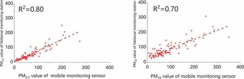
Due to the variation in the environmental and meteorological conditions across the different districts, the concentration measured by the sensors should be calibrated. Before being installed in taxis, the PM monitors were calibrated according to the calibration specification (General Administration of Quality Supervision 2017). After monitoring, the correlations between the daily average PM concentration by national monitoring stations and that by mobile monitoring were analyzed (Figure 3). Since the national monitoring stations only measure PM_2.5 and PM₁₀, we could only carry out correlation analysis on these two kinds of particles. The coefficient of determination (R²) of PM_2.5 was 0.80 and that of PM₁₀ was 0.70, which indicated that the accuracy of the mobile monitoring sensor was good.

Figure 3. Correlation of the daily average PM value between mobile monitors and national monitoring stations.

Overall distribution characteristics of PMs

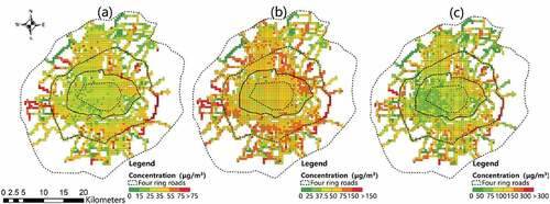
The average concentrations of PM₁, PM_2.5 and PM₁₀ were 36.53, 68.85 and 99.93 μg/m³, respectively, during the monitoring period. The overall spatial distribution patterns of PM after normalization and classification according to the air quality guidelines of the World Health Organization (WHO) (WHO 2005) are shown in Figure 4. High concentrations of the three kinds of PM were distributed in the suburbs, while relatively low concentrations were concentrated in the central area. Additionally, although the concentration distribution pattern of PM_2.5 was consistent with that of PM₁ and PM₁₀, there were more heavily polluted areas of PM_2.5.

Figure 4. Spatial distribution patterns of PM₁ (a), PM_2.5 (b), and PM₁₀ (c).

Spatial pattern of PM concentrations

PM concentrations along different road directions and among various road grades

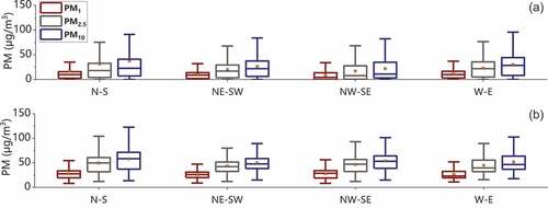
The PM concentrations of 95 days excluding outliers were selected as the database for further analysis. The PM distribution patterns across different road grades and directions were analyzed by selecting data with wind speeds greater than 2 m/s. The dominant wind direction of Shenyang in winter is northwest and southwest. From the boxplots of concentration variations, when the wind direction was N‒NNW, the concentrations of the three kinds of PMs in the four road directions were ranked as follows: NW‒SE<NE‒SW<W‒E<N‒S (Figure 5(a)). When the wind direction was SW‒WSW, the concentrations of the three kinds of PMs were as follows: NE‒SW<W‒E<NW‒SE<N‒S (Figure 5(b)). The results indicated that roads parallel to the dominant wind directions had the lowest concentrations. Additionally, the impact of road direction on PM10 was greater than that on the other two pollutants. In the northwest wind direction, the difference in the PM10 concentration between roads parallel to the dominant wind direction and other roads was 15.64 μg/m3. The PM10 concentration of roads parallel to the dominant wind direction was significantly higher than that of other roads (p <0.001). The impact of road grades on PM was very small. Mainly because of the complexity of the intraurban environment, many factors have a greater impact than road grades, resulting in no significant difference in the concentration of PM among various road grades under the same air quality (p >0.05).

Figure 5. PM concentrations along different road directions under dominant wind directions. (a) N‒NNW wind direction; (b) SW‒WSW wind direction.

PM concentrations within various ring roads

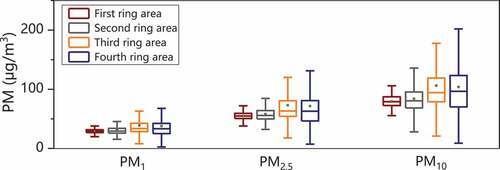
To compare the distribution characteristics of the PM concentrations in different ring roads, the original PM concentration data of 95 days were used for analysis. From the first ring road area to the fourth, the average PM₁ concentrations were 29.13, 30.62, 38.78 and 37.97 μg/m³, respectively; the average PM_2.5 concentrations were 54.84, 58.11, 72.98 and 71.55 μg/m³, respectively; and the average PM₁₀ concentrations were 79.51, 84.04, 106.03 and 103.85 μg/m³, respectively (Figure 6). The PM concentrations outside the second ring road were much higher than those inside the second ring road (P <0.001).

Figure 6. PM concentrations within various ring roads.

PM concentrations among various urban functional zones

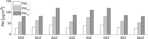
The PM concentrations in the AGZ, DEZ and INZ were higher than those in the other types of UFZs. The concentrations of PM₁, PM_2.5 and PM₁₀ were 27.89–43.79, 54.03–82.29 and 82.68–120.54 μg/m³, respectively (Figure 7). The PM concentrations in the AGZ were significantly higher than those in the EDZ, GSZ and REZ (p <0.05). The PM concentrations measured in the INZ were obviously higher than those in the EDZ, GSZ and REZ (p <0.05). The average concentration level of PM_2.5 in the INZ was 1.36 times that in the EDZ, 1.28 times that in the REZ, and 1.34 times that in the GSZ, which were all higher than the 24-hour guideline (75 μg/m³) of the National Ambient Air Quality Standards (GB 3095–2012) (NAAQS).

Figure 7. PM concentrations among various urban functional zones. EDZ: educational land zone; BUZ: business zone; AGZ: agricultural zone; GSZ: green space zone; INZ: industrial zone; DEZ: development zone; REZ: residential zone; WAZ: water zone.

Spatial cluster and spatial outlier analyses

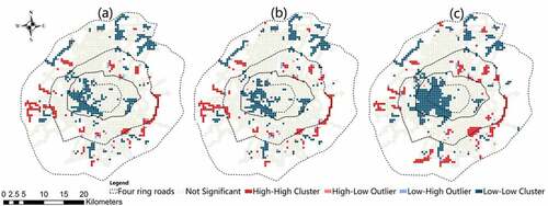
In the spatial autocorrelation analysis, the global Moran’s I index of PM₁, PM_2.5, and PM₁₀ was 0.37 (p < 0.001), 0.36 (p < 0.001), and 0.43 (p < 0.001), respectively, indicating that PM has strong and significant spatial autocorrelation. The local autocorrelation of the three pollutants was analyzed by using the local Moran’s I index. The proportions of spatial autocorrelation areas of PM₁, PM_2.5, and PM₁₀ to the total area were 23.77%, 23.58% and 29.77%, respectively (Figure 8). The spatial autocorrelation of PM₁₀ was higher than that of PM₁ and PM_2.5, and the LL area of PM₁₀ was larger than that of the other two pollutants. HH areas were mainly distributed in the east and west of the city near the third ring road, while LL areas mainly occurred in the west of the second ring road and the north outside the third ring road.

Figure 8. Spatial autocorrelation of PM in the study area. (a) PM₁; (b) PM_2.5; and (c) PM₁₀.

Analysis of influencing factors

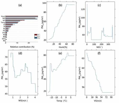
The relative contributions of 13 factors to PM were analyzed by the BRT method (Figure 9). Meteorological factors (Humi, WD, WS and Temp) constituted the most important influencing factors of the three pollutants, accounting for more than 80% of the relative contribution rate. The other social and landscape pattern factors only provided a 20% relative contribution to the PM concentration. The marginal effects showed that the PM concentration has a positive correlation with Humi and Temp and a negative correlation with WS and VS. When the vehicle speed reached 54 km/h, the concentration of PM tended to stabilize. When WD is oriented in the dominant direction, the PM concentration is lower than the average level.

Figure 9. Relative contribution of each factor to PM concentrations (a) and marginal effects of five dominant factors on PM_2.5 (b-f). Humi: relative humidity; WD: wind direction; WS: wind speed; Temp: temperature; VS: vehicle speed; TR: time range; BC: betweenness centrality; HC: heating capacity of heating supply companies; UFZ: urban functional zone; RD: road direction; BD: building density; DCC: distance from the city center; RG: road grade.

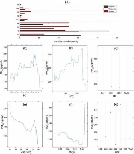
As regional meteorological factors cannot be controlled by humans, this study aims to provide a basis for the treatment of air pollution control by analyzing other influencing factors of PM under different AQI conditions. We assume that the meteorological conditions observed on the same day are the same, and the social and landscape pattern factors were the main factors affecting the pollutant distribution pattern at this time. The monitoring data under three kinds of AQI conditions (excellent, moderate pollution, and serious pollution) were selected to analyze the relative contributions of the social and landscape pattern factors to the measured PM concentration. Through previous analysis, it was found that the relative contribution ranking of influencing factors of different particles is consistent, so we use PM_2.5 as an example to analyze the influence of social and landscape pattern factors on the distribution of air pollutants.

Under excellent air quality conditions, VS and TR were the main contributing factors, with contribution rates of 31.48% and 30.57%, respectively. Under moderate pollution, TR was the main contributing factor, with a contribution rate of 45.69%. Under serious pollution, BC, HC and TR were the main contributing factors, with contribution rates of 25.47%, 25.45%, and 23.48%, respectively (Figure 10). Combined with different weather conditions, TR, VS, BC and HC were the major factors affecting PM. Taking serious pollution weather as an example, the relationship between each factor and pollutant can be seen from the marginal effect diagram. BC and HC were positively correlated with the measured PM_2.5 concentrations. For different time ranges, night had a significant influence. For different UFZs, the INZ had the greatest impact on PM_2.5 pollution, followed by the AGZ.

Figure 10. Relative contribution of influencing factors to PM_2.5 concentration under three air quality conditions (a) and marginal effects of six dominant factors on PM_2.5 under serious pollution (b-g). RG: road grade; DCC: distance from the city center; BD: building density; RD: road direction; UFZ: urban functional zone; HC: heating capacity of heating supply companies; BC: betweenness centrality; TR: time range; VS: vehicle speed.

Discussion

Distribution pattern of PM concentrations

In this study, the distribution pattern of the three PM concentration groups demonstrated that the PM concentration within the second ring was lower than that outside the second ring. The regions with high concentrations of PM were mainly concentrated between the second and fourth ring areas. In contrast, the concentration within the second ring area was generally low. This was mainly because the high concentration regions of PM were mainly concentrated in Shenyang’s industrial areas or bare land areas between the second and fourth ring areas, such as the Tiexi heavy industrial park in the west and the Hunnan logistics park in the south. Our results were in contrast to several previous studies, such as those completed in New York (Ross et al. 2007), Beijing (Kong and Tian 2020) and Shanghai (Liu et al. 2016), where the concentration of air pollutants in urban areas was higher than that in suburban areas. This inconsistency could be explained by the differences in the distance to the sea, the elevation of the studied area, the monitoring data resolution and the research scale. In particular, the study of urban air pollution using fixed monitoring stations is based on a limited number of observational stations, which often cannot reflect the real urban internal distribution pattern of air pollutants (Zhou and Lin 2019).

The degree of air pollution varies within different functional zones. Industrial zones with some factories can discharge many air pollutants (Fan et al. 2021; Mardones and Sanhueza 2015; Merbitz, Fritz, and Schneider 2012); residential and commercial zones are often recognized as nonpoint sources of air pollution due to the effect of intense human activities, while green space and water bodies can absorb and purify air pollution (Chen et al. 2019; Lei et al. 2018; Zhu and Zhou 2019). We found that the AGZ, DEZ and INZ had higher PM concentration values than the other types of UFZs, and the GSZ and WAZ had lower PM concentrations. Therefore, we should pay attention to the control of atmospheric PM in industrial areas and alleviate urban air pollution by adjusting the industrial structure, optimizing the industrial layout and using clean energy (Cai et al. 2018). Additionally, we should comprehensively consider the layout of open space (square, park, green space, etc.) and urban water to alleviate the pollution problem.

Influencing factors of intraurban PM concentrations

Due to the changeable local microclimate, complex landscape pattern and intense human activities, many factors may affect the air pollution pattern inside a city, such as meteorological factors, land use patterns, traffic conditions, building heights, building densities, canopy heights, etc. (Tecer et al. 2008). Our BRT analysis showed that meteorological conditions (temperature, humidity, wind) contributed more than 80% to PM pollution in Shenyang city. The marginal effects indicated that the PM_2.5 concentration was positively correlated with temperature and humidity and negatively correlated with wind speed (Figure 9). Our results were consistent with previous findings (Kang et al. 2020), demonstrating that climate is the dominant factor influencing PM pollution (Yang et al. 2018). Our results were comparable to those of a study completed in Beijing during the winter heating period, which showed that relative humidity was the most important factor affecting the PM_2.5 concentration, with a contribution rate of 41%. The dilution contribution of northerly wind was 27.8% (Meng et al. 2019).

In addition to meteorological conditions, landscape patterns and social factors also exert considerable influences on PM pollution (Li et al. 2020). Our BRT analysis under various pollution conditions (excellent, moderate and serious) showed that BC, HC, TR and VS were the major factors affecting the PM concentration (Figure 10(a)). The marginal effects indicated that the PM_2.5 concentration was positively correlated with BC and HC and negatively correlated with VS (Figure 10(b)). BC and HC represent the line source pollution of roads and point source pollution of cities, respectively. Researchers have found that there is a positive correlation between BC and PM. In some areas of China, an average increase of 1.1% in the PM concentration would be caused by an increase of 1% in the BC value at night (Zhou and Lin 2019). Another important social factor is the use of HC. In Shenyang, more than half of the coal is used for heating in winter. Studies have shown that the reduction of coal use can greatly improve air quality (Yuan et al. 2018). We should optimize the energy structure and increase the use of clean energy. VS is an indicator of traffic jam severity. Our results were consistent with previous findings demonstrating that the degree of traffic jamming is related to the PM concentration. In other words, the increase in fuel consumption per unit road area leads to an increase in the PM concentration (Li and Mao 2020). In the study of PM concentrations measured in different time periods, many studies reached a similar conclusion. In the study of PM in Guangzhou, China, it was noted that the median concentration of PM_2.5 in the evening rush hour was much higher than that in the morning. The reason for the different concentrations across different time periods is that industrial production, daily life, transportation, etc., continued to operate for several hours during the day, each functional area induced an increase in PM, and its cumulative effect was obvious at night (Zhou and Lin 2019).

In addition to the main influencing factors mentioned above, the overall influence of urban landscape pattern factors on the distribution of PM throughout the whole city is small, but the influence of building height, building density or building form on the concentration distribution of pollutants at the microscale (blocks or single buildings) will become increasingly significant (Ling, Candice Lung, and Uhrner 2020). Transportation-related facilities are generally regarded as important air pollution sources; most researchers focus on the impact of road length, road density, and traffic flow on urban air quality (Ling, Candice Lung, and Uhrner 2020; Liu et al. 2016; Wei et al. 2020), and the effect of road direction and wind direction on fine particles is rarely mentioned. Our results demonstrated the strong relationships of the concentrations of PM along road directions and the dominant wind direction. Our findings provide important insights for wind corridor construction and road planning in the future. To alleviate air pollution, wind corridors should be constructed parallel to the dominant wind direction. In addition, in unplanned urban‒rural transition areas, industrial land should be arranged in the downwind direction of the city’s dominant wind, and the direction of the surrounding roads should be adjusted to facilitate the diffusion of pollutants.

Advantages and limitations

Compared with ordinary mobile monitoring and national fixed monitoring stations, the taxi monitoring method used in this study could obtain higher spatial-temporal resolution data at a lower cost to capture dynamic air pollution distribution patterns. However, taxi monitoring is carried out on roads with random routes, and traffic congestion and exhaust emissions may have a certain impact on the measured concentrations of PM (Wei et al. 2020). Previous research revealed that the PM_2.5 concentration of traffic stations is 17–18% higher than that of urban background stations (Hoek et al. 2002). However, since all monitoring data were located on roads, the monitoring results could still reveal the distribution patterns of PM concentrations and expose the hot and cold spots of pollution. Additionally, we will consider more detailed meteorological data in future research. The mobile monitoring scheme proposed in this study is still an efficient and feasible monitoring method for urban air pollution, which can provide a scientific basis for the development of a warning system for air pollution hot spots and for the planning of air pollution prevention and control. Low-cost and high-efficiency taxi monitoring was used to visualize the temporal and spatial variations in PM pollution in the city with high resolution. The monitoring means and modeling methods we proposed have important reference significance for future urban planning. This method could also be extended to more pollutants and other cities to interpret urban environmental problems.

Conclusions

In this study, five taxis equipped with mobile monitors were used to monitor the concentration of urban PM in winter over five months. Normalized monitoring data were used to analyze the spatial distribution patterns of PM₁, PM_2.5 and PM₁₀. The PM concentration characteristics of different road grades, road directions, road rings, dominant wind directions and UFZs were analyzed. Global Moran’s I and local Moran’s I were applied to investigate the spatial aggregation of the three PMs. The results indicated that the concentration distribution pattern of PM in the Shenyang urban area is low in the central urban area and high in the suburbs. The PM concentrations outside the second ring road were much higher than those inside the second ring road. The impact of RG on the measured PM concentration was very small, but the road direction parallel to the dominant wind directions has the lowest concentration. For the different UFZs, the AGZ, DEZ and INZ had higher concentration values among the eight types, and the GSZ and WAZ had lower concentration values. All three kinds of particles exhibited spatial autocorrelation, and the spatial autocorrelation of PM₁₀ was higher than that of PM₁ and PM_2.5. The BRT method was used to analyze the relative contributions of 13 meteorological, social and landscape pattern factors to the PM concentration. Meteorological factors play an important role in the PM concentration. The urban air quality monitoring method based on taxis in this study is fast and convenient and provides real-time and effective support for urban air pollution warnings. Additionally, using high spatial-temporal resolution monitoring data to analyze the spatial pattern of pollutants can be used to effectively identify high-risk areas of pollution and provide guidance for the construction of urban ventilation corridors and the setting of air pollution control measures.

Disclosure statement

No potential conflict of interest was reported by the author(s).

Additional information

Funding

Funding for this project was provided by the National Natural Science Foundation of China (Nos. 41730647 and 32071580).

References

- Baccarelli, A., F. Barretta, C. Dou, X. Zhang, J. P. McCracken, A. Diaz, P. A. Bertazzi, J. Schwartz, S. Wang, and L. F. Hou. 2011. “Effects of Particulate Air Pollution on Blood Pressure in a Highly Exposed Population in Beijing, China: A Repeated-Measure Study.” Environmental Health : A Global Access Science Source 10 (1): 10. doi:10.1186/1476-069X-10-108.
- Bai, L., Z. J. He, S. Y. Ni, W. Y. Chen, N. Li, and S. Y. Sun. 2019. “Investigation of PM2.5 Absorbed with Heavy Metal Elements, Source Apportionment and Their Health Impacts in Residential Houses in the North-East Region of China.” Sustainable Cities and Society 51: 9. doi:10.1016/j.scs.2019.101690.
- Briggs, D. J., S. Collins, P. Elliott, P. Fischer, S. Kingham, E. Lebret, K. Pryl, H. VanReeuwijk, K. Smallbone, and A. VanderVeen. 1997. “Mapping Urban Air Pollution Using GIS: A Regression-Based Approach.” International Journal of Geographical Information Science : IJGIS 11 (7): 699–14.
- Cai, S., Q. Ma, S. Wang, B. Zhao, M. Brauer, A. Cohen, R. V. Martin, et al. 2018. “Impact of Air Pollution Control Policies on Future PM2.5 Concentrations and Their Source Contributions in China.” Journal of Environmental Management 227: 124–133.
- Cai, W. H., J. Yang, Z. H. Liu, Y. M. Hu, and P. J. Weisberg. 2013. “Post-Fire Tree Recruitment of a Boreal Larch Forest in Northeast China.” Forest Ecology and Management 307: 20–29. doi:10.1016/j.foreco.2013.06.056.
- Chen, Z. Y., D. L. Chen, C. F. Zhao, M. P. Kwan, J. Cai, Y. Zhuang, B. Zhao, et al. 2020. “Influence of Meteorological Conditions on PM2.5 Concentrations Across China: A Review of Methodology and Mechanism.” Environment International. 139: 105558.
- Chen, M., F. Dai, B. Yang, and S. W. Zhu. 2019. “Effects of Urban Green Space Morphological Pattern on Variation of PM2.5 Concentration in the Neighborhoods of Five Chinese Megacities.” Building and Environment 158: 1–15. doi:10.1016/j.buildenv.2019.04.058.
- Chen, W., H. Ran, X. Cao, J. Wang, D. Teng, J. Chen, and X. Zheng. 2020. “Estimating PM2.5 with High-Resolution 1-Km AOD Data and an Improved Machine Learning Model Over Shenzhen, China.” The Science of the Total Environment 746: 141093. doi:10.1016/j.scitotenv.2020.141093.
- Chen, Y., W. Yue, and D. La Rosa. 2020. “Which Communities Have Better Accessibility to Green Space? An Investigation into Environmental Inequality Using Big Data.” Landscape and Urban Planning 204: 103919. doi:10.1016/j.landurbplan.2020.103919.
- Clark, L. P., D. B. Millet, and J. D. Marshall. 2011. “Air Quality and Urban Form in US Urban Areas: Evidence from Regulatory Monitors.” Environmental Science & Technology 45 (16): 7028–7035.
- de Hartog, J. J., G. Hoek, A. Mirme, T. Tuch, G. P. A. Kos, H. M. ten Brink, B. Brunekreef, et al. 2005. “Relationship Between Different Size Classes of Particulate Matter and Meteorology in Three European Cities.” Journal of Environmental Monitoring : JEM 7 (4): 302–310.
- Demuzere, M., R. M. Trigo, J.-V.-G. de Arellano, and N. P. M. van Lipzig. 2009. “The Impact of Weather and Atmospheric Circulation on O-3 and PM10 Levels at a Rural Mid-Latitude Site.” Atmospheric Chemistry and Physics 9 (8): 2695–2714.
- Fan, H., C. F. Zhao, and Y. K. Yang. 2020. “A Comprehensive Analysis of the Spatio-Temporal Variation of Urban Air Pollution in China During 2014-2018.” Atmospheric Environment. 220: 117066.
- Fan, H., C. F. Zhao, Y. K. Yang, X. C. Yang, and C. Y. Wang. 2021. “Impact of Emissions from a Single Urban Source on Air Quality Estimated from Mobile Observation and WRF-STILT Model Simulations.” Air Quality, Atmosphere, & Health 14 (9): 1313–1323.
- Filonchyk, M., and H. W. Yan. 2018. “The Characteristics of Air Pollutants During Different Seasons in the Urban Area of Lanzhou, Northwest China.” Environmental Earth Sciences 77 (22): 1–17.
- Freeman, L. C. 1977. “Set of Measures of Centrality Based on Betweenness.” Sociometry 40 (1): 35–41.
- Froeschke, J. T., and B. F. Froeschke. 2011. “Spatio-Temporal Predictive Model Based on Environmental Factors for Juvenile Spotted Seatrout in Texas Estuaries Using Boosted Regression Trees.” Fisheries Research 111 (3): 131–138.
- Fu, M., J. A. Kelly, and J. P. Clinch. 2020. “Prediction of PM2.5 Daily Concentrations for Grid Points Throughout a Vast Area Using Remote Sensing Data and an Improved Dynamic Spatial Panel Model.” Atmospheric Environment 237: 117667.
- General Administration of Quality Supervision, I.a.Q.o.t.P.s.R.o.C. 2017. Calibration Specification for PM2.5 Mass Concentration Measurement Instruments. Beijing: China Quality Inspection Publisher.
- Golden, H. E., C. R. Lane, A. G. Prues, and E. D’Amico. 2016. “Boosted Regression Tree Models to Explain Watershed Nutrient Concentrations and Biological Condition.” Journal of the American Water Resources Association / AWRA 52 (5): 1251–1274.
- Guo, B., X. Wang, L. Pei, Y. Su, D. Zhang, and Y. Wang. 2021. “Identifying the Spatiotemporal Dynamic of PM2.5 Concentrations at Multiple Scales Using Geographically and Temporally Weighted Regression Model Across China During 2015-2018.” The Science of the Total Environment 751: 141765.
- He, W., S. Zhang, H. Meng, J. Han, G. Zhou, H. Song, S. Zhou, and H. Zheng. 2022. “Full-Coverage PM2.5 Mapping and Variation Assessment During the Three-Year Blue-Sky Action Plan Based on a Daily Adaptive Modeling Approach.” Remote Sensing 14 (15): 3571.
- Ho, C.-C., C.-C. Chan, C.-W. Cho, H.-I. Lin, J.-H. Lee, and C.-F. Wu. 2015. “Land Use Regression Modeling with Vertical Distribution Measurements for Fine Particulate Matter and Elements in an Urban Area.” Atmospheric Environment 104: 256–263. doi:10.1016/j.atmosenv.2015.01.024.
- Hoek, G., R. Beelen, K. de Hoogh, D. Vienneau, J. Gulliver, P. Fischer, and D. Briggs. 2008. “A Review of Land-Use Regression Models to Assess Spatial Variation of Outdoor Air Pollution.” Atmospheric Environment 42 (33): 7561–7578. doi:10.1016/j.atmosenv.2008.05.057.
- Hoek, G., K. Meliefste, J. Cyrys, M. Lewne, T. Bellander, M. Brauer, P. Fischer, et al. 2002. “Spatial Variability of Fine Particle Concentrations in Three European Areas.” Atmospheric Environment 36 (25): 4077–4088. doi:10.1016/S1352-2310(02)00297-2.
- Huang, Y. Y., Q. W. Yan, and C. A. R. Zhang. 2018. “Spatial-Temporal Distribution Characteristics of PM2.5 in China in 2016.” Journal of Geovisualization and Spatial Analysis 2 (2): 1–18.
- Kang, N., F. Deng, R. Khan, K. R. Kumar, K. Hu, X. Yu, X. Wang, and N. S. M. P. Latha Devi. 2020. “Temporal Variations of PM Concentrations, and Its Association with AOD and Meteorology Observed in Nanjing During the Autumn and Winter Seasons of 2014–2017.” Journal of Atmospheric and Solar-Terrestrial Physics 203: 105273.
- Kong, L., and G. Tian. 2020. “Assessment of the Spatio-Temporal Pattern of PM2.5 and Its Driving Factors Using a Land Use Regression Model in Beijing, China.” Environmental Monitoring and Assessment 192 (2): 95. doi:10.1007/s10661-019-7943-9.
- Kwag, Y., M.-H. Kim, J. Oh, S. Shah, S. Ye, and E.-H. Ha. 2021. “Effect of Heat Waves and Fine Particulate Matter on Preterm Births in Korea from 2010 to 2016.” Environment International 147: 106239. doi:10.1016/j.envint.2020.106239.
- Leathwick, J. R., J. Elith, M. P. Francis, T. Hastie, and P. Taylor. 2006. “Variation in Demersal Fish Species Richness in the Oceans Surrounding New Zealand: An Analysis Using Boosted Regression Trees.” Marine Ecology Progress Series 321: 267–281.
- Lee, M., M. Brauer, P. Wong, R. Tang, T. H. Tsui, C. Choi, W. Cheng, et al. 2017. “Land Use Regression Modelling of Air Pollution in High Density High Rise Cities: A Case Study in Hong Kong.” The Science of the Total Environment 592: 306–315.
- Lei, Y. K., Y. B. Duan, D. He, X. W. Zhang, L. Q. Chen, Y. H. Li, Y. G. Gao, G. H. Tian, and J. B. Zheng. 2018. “Effects of Urban Greenspace Patterns on Particulate Matter Pollution in Metropolitan Zhengzhou in Henan, China.” Atmosphere 9 (5): 15. doi:10.3390/atmos9050199.
- Li, C. L., M. Liu, Y. M. Hu, T. Shi, X. Q. Qu, and M. T. Walter. 2018. “Effects of Urbanization on Direct Runoff Characteristics in Urban Functional Zones.” The Science of the Total Environment 643: 301–311.
- Li, C., M. Liu, Y. Hu, R. Zhou, N. Huang, W. Wu, and C. Liu. 2020. “Spatial Distribution Characteristics of Gaseous Pollutants and Particulate Matter Inside a City in the Heating Season of Northeast China.” Sustainable Cities and Society 61: 102302.
- Li, M., and C. Mao. 2020. “Spatial Effect of Industrial Energy Consumption Structure and Transportation on Haze Pollution in Beijing-Tianjin-Hebei Region.” International Journal of Environmental Research and Public Health 17 (15): 5610.
- Ling, H., S. C. Candice Lung, and U. Uhrner. 2020. “Micro-Scale Particle Simulation and Traffic-Related Particle Exposure Assessment in an Asian Residential Community.” Environmental Pollution (Barking, Essex : 1987) 266 (Pt 2): 115046.
- Li, X. L., G. Q. Tang, L. G. Li, W. J. Quan, Y. F. Wang, Z. Q. Zhao, N. W. Liu, Y. Hong, and Y. J. Ma. 2022. “Multilevel Air Quality Evolution in Shenyang: Impact of Elevated Point Emission Reduction.” Journal of Environmental Sciences 113: 300–310. doi:10.1016/j.jes.2021.05.039.
- Liu, J., W. Cai, S. Zhu, and F. Dai. 2020. “Impacts of Vehicle Emission from a Major Road on Spatiotemporal Variations of Neighborhood Particulate Pollution—a Case Study in a University Campus.” Sustainable Cities and Society 53: 101917.
- Liu, C., B. H. Henderson, D. Wang, X. Yang, and Z. R. Peng. 2016. “A Land Use Regression Application into Assessing Spatial Variation of Intra-Urban Fine Particulate Matter (PM2.5) and Nitrogen Dioxide (NO2) Concentrations in City of Shanghai, China.” The Science of the Total Environment 565: 607–615.
- Liu, M., Y. M. Hu, and C. L. Li. 2017. “Landscape Metrics for Three-Dimensional Urban Building Pattern Recognition.” Applied Geography 87: 66–72.
- Mardones, C., and L. Sanhueza. 2015. “Tradable Permit System for PM2.5 Emissions from Residential and Industrial Sources.” Journal of Environmental Management 157: 326–331.
- Meng, C., T. Cheng, X. Gu, S. Shi, W. Wang, Y. Wu, and F. Bao. 2019. “Contribution of Meteorological Factors to Particulate Pollution During Winters in Beijing.” The Science of the Total Environment 656: 977–985.
- MEP. 2012. Technical Regulation on Ambient Air Quality Index(on trial).
- Merbitz, H., S. Fritz, and C. Schneider. 2012. “Mobile Measurements and Regression Modeling of the Spatial Particulate Matter Variability in an Urban Area.” The Science of the Total Environment 438: 389–403.
- Messier, K. P., S. E. Chambliss, S. Gani, R. Alvarez, M. Brauer, J. J. Choi, S. P. Hamburg, et al. 2018. “Mapping Air Pollution with Google Street View Cars: Efficient Approaches with Mobile Monitoring and Land Use Regression.” Environmental Science & Technology 52 (21): 12563–12572.
- Miller, K. A., D. S. Siscovick, L. Sheppard, K. Shepherd, J. H. Sullivan, G. L. Anderson, and J. D. Kaufman. 2007. “Long-Term Exposure to Air Pollution and Incidence of Cardiovascular Events in Women.” The New England Journal of Medicine 356 (5): 447–458.
- Porta, S., E. Strano, V. Iacoviello, R. Messora, V. Latora, A. Cardillo, F. H. Wang, and S. Scellato. 2009. “Street Centrality and Densities of Retail and Services in Bologna, Italy.” Environment and Planning B: Planning and Design 36 (3): 450–465.
- Ross, Z., M. Jerrett, K. Ito, B. Tempalski, and G. Thurston. 2007. “A Land Use Regression for Predicting Fine Particulate Matter Concentrations in the New York City Region.” Atmospheric Environment 41 (11): 2255–2269.
- Sajani, S. Z., S. Marchesi, A. Trentini, D. Bacco, C. Zigola, S. Rovelli, I. Ricciardelli, et al. 2018. “Vertical Variation of PM2.5 Mass and Chemical Composition, Particle Size Distribution, NO2, and BTEX at a High Rise Building.” Environmental Pollution (Barking, Essex : 1987) 235: 339–349.
- Shahpoury, P., Z. W. Zhang, A. Arangio, V. Celo, E. Dabek-Zlotorzynska, T. Harner, and A. Nenes. 2021. “The Influence of Chemical Composition, Aerosol Acidity, and Metal Dissolution on the Oxidative Potential of Fine Particulate Matter and Redox Potential of the Lung Lining Fluid.” Environment International 148: 106343.
- Shi, Y., X. Xie, J.-C.-H. Fung, and E. Ng. 2018. “Identifying Critical Building Morphological Design Factors of Street-Level Air Pollution Dispersion in High-Density Built Environment Using Mobile Monitoring.” Building and Environment 128: 248–259.
- Shi, X. Q., C. F. Zhao, J. H. Jiang, C. Y. Wang, X. Yang, and Y. L. Yung. 2018. “Spatial Representativeness of PM2.5 Concentrations Obtained Using Observations from Network Stations.” Journal of Geophysical Research-Atmospheres 123 (6): 3145–3158.
- Song, J., C. L. Li, M. Liu, Y. M. Hu, and W. Wu. 2022. “Spatiotemporal Distribution Patterns and Exposure Risks of PM2.5 Pollution in China.” Remote Sensing 14 (13): 3173.
- Stowell, J. D., J. Bi, M. Z. Al-Hamdan, H. J. Lee, S.-M. Lee, F. Freedman, P. L. Kinney, and Y. Liu. 2020. “Estimating PM2.5 in Southern California Using Satellite Data: Factors That Affect Model Performance.” Environmental Research Letters 15 (9): 094004.
- Tecer, L. H., P. Suren, O. Alagha, F. Karaca, and G. Tuncel. 2008. “Effect of Meteorological Parameters on Fine and Coarse Particulate Matter Mass Concentration in a Coal-Mining Area in Zonguldak.” Turkey Journal of the Air & Waste Management Association 58 (4): 543–552.
- Wang, F., A. Antipova, and S. Porta. 2011. “Street Centrality and Land Use Intensity in Baton Rouge, Louisiana.” Journal of Transport Geography 19 (2): 285–293.
- Wang, Q., Z. S. Dong, Y. Guo, F. Yu, Z. Y. Zhang, and R. Q. Zhang. 2020. “Characterization of PM2.5-Bound Polycyclic Aromatic Hydrocarbons at Two Central China Cities: Seasonal Variation.” Sources, and Health Risk Assessment Archives of Environmental Contamination and Toxicology 78 (1): 20–33.
- Wan, Y., Y. H. Li, C. H. Liu, and Z. Q. Li. 2020. “Is Traffic Accident Related to Air Pollution? A Case Report from an Island of Taihu Lake, China.” Atmospheric Pollution Research 11 (5): 1028–1033.
- Wei, T., B. Wijesiri, Y. Li, and A. Goonetilleke. 2020. “Particulate Matter Exchange Between Atmosphere and Roads Surfaces in Urban Areas.” Journal of Environmental Sciences 98: 118–123.
- WHO. 2005. WHO Air Quality Guidelines for Particulate Matter, Ozone, Nitrogen, Dioxide and Sulfur Dioxide. Global Update 2005, Summary of Risk Assessment. Switzerland: WHO Press.
- Xue, T., J. Liu, Q. Zhang, G. N. Geng, Y. X. Zheng, D. Tong, Z. Liu, et al. 2019. “Rapid Improvement of PM2.5 Pollution and Associated Health Benefits in China During 2013-2017.” Science China Earth Sciences 62 (12): 1847–1856.
- Yang, D., X. Wang, J. Xu, C. Xu, D. Lu, C. Ye, Z. Wang, and L. Bai. 2018. “Quantifying the Influence of Natural and Socioeconomic Factors and Their Interactive Impact on PM2.5 Pollution in China.” Environmental Pollution (Barking, Essex : 1987) 241: 475–483.
- Yang, X. C., Y. Wang, C. F. Zhao, H. Fan, Y. K. Yang, Y. L. Chi, L. X. Shen, and X. Yan. 2022. “Health Risk and Disease Burden Attributable to Long-Term Global Fine-Mode Particles.” Chemosphere 287: 132435.
- Yu, W. H. 2017. “Assessing the Implications of the Recent Community Opening Policy on the Street Centrality in China: A GIS-Based Method and Case Study.” Applied Geography 89: 61–76.
- Yuan, J., C. Na, Q. Lei, M. Xiong, J. Guo, and Z. Hu. 2018. “Coal Use for Power Generation in China.” Resources, Conservation and Recycling 129: 443–453.
- Zeng, Y. Y., Y. F. Cao, X. Qiao, B. C. Seyler, and Y. Tang. 2019. “Air Pollution Reduction in China: Recent Success but Great Challenge for the Future.” The Science of the Total Environment 663: 329–337.
- Zhang, K. Y., C. F. Zhao, H. Fan, Y. K. Yang, and Y. Sun. 2020. “Toward Understanding the Differences of Pm(2.5)Characteristics Among Five China Urban Cities.” Asia-Pacific Journal of Atmospheric Sciences 56 (4): 493–502.
- Zhao, C. F., Y. Wang, X. Q. Shi, D. Z. Zhang, C. Y. Wang, J. H. Jiang, Q. Zhang, and H. Fan. 2019. “Estimating the Contribution of Local Primary Emissions to Particulate Pollution Using High-Density Station Observations.” Journal of Geophysical Research-Atmospheres 124 (3): 1648–1661.
- Zhao, Y., Y.-C. Zhang, and I. Destech Publicat. 2016. “Study on Ecological Environmental Problems and Their Countermeasures in the Process of Rural Urbanization.“
- Zhou, S. H., and R. P. Lin. 2019. “Spatial-Temporal Heterogeneity of Air Pollution: The Relationship Between Built Environment and On-Road PM2.5 at Micro Scale.” Transportation Research Part D: Transport and Environment 76: 305–322.
- Zhu, D., and X. F. Zhou. 2019. “Effect of Urban Water Bodies on Distribution Characteristics of Particulate Matters and NO2.” Sustainable Cities and Society 50: 10.