Scalable near-repeat and event chain calculations over heterogeneous computer architecture and systems

Abstract

As a case of space–time interaction, near-repeat calculation indicates that when an event takes place at a certain location, its immediate geographical surroundings would face an increased risk of experiencing subsequent events within a fairly short period of time. This paper presents an exploratory study that extends the investigation of the near-repeat phenomena to a series of space–time interaction, namely event chain calculation. Existing near-repeat tools can only deal with a limited amount of data due to computation constraints, let alone the event chain analysis. By deploying the modern accelerator technology and hybrid computer systems, this study demonstrates that large-scale near-repeat calculation or event chain analysis can be partially resolved through high-performance computing solutions to advance such a challenging statistical problem in both spatial analysis and crime geography.

Keywords:

• Parallel and high-performance computing
• near-repeat
• event chain analysis
• crime analysis

1. Introduction

There is a growing consensus that the spatial and temporal dimensions of the data should be handled jointly instead of treated independently (Andrienko et al., 2010; Anselin, 2012; Goodchild, 2009; Goodchild & Janelle, 2004). Ignoring these interdependence leads to the overlooking of many possible interactions and might cause biases in the analytical results (Ye & Rey, 2013). Researchers thus have to consider modelling approaches that effectively integrate spatial and temporal aspects of the data (Andrienko & Andrienko, 2013). Near-repeat is a special phenomenon conceptualized based on possible linkages in the spatial and temporal dimensions of events. It means that after an event occurs at a certain location, its immediate surroundings would face an increased risk of experiencing subsequent events within a fairly short period of time (Ratcliffe & Rengert, 2008; Wells, Wu, & Ye, 2011). This statistical analysis can be considered as a before-and-after analysis of a specific type of event in any specific location and its locale. The assumption is that the space–time pattern of such events at any location and its vicinity is random before an incident occurs. After an incident, a spatial cluster of follow-up events is expected physically close to the target of the initial incident (Henriksen, Mattick, & Fisher, 2016). The conclusion derived from near-repeat is policy-relevant in the spatial crime research, because it can suggest interventions that might prevent possible subsequent crimes. For example, the police department could adjust patrol activities according to the risk level (Ye & Liu, 2012). Evidence of repeat and near-repeat phenomena has primarily been observed on burglaries (Johnson, Summers, & Pease, 2009; Townsley, Homel, & Chaseling, 2000). Researchers also investigated gun violence (Ratcliffe & Rengert, 2008; Wells et al., 2011).

Developed by Ratcliffe and Rengert (2008), the near-repeat calculator was implemented to identify whether significant space–time clustering exists among a group of events. This software adopts a revised Knox test (Knox & Bartlett, 1964) and Monte Carlo simulation to examine such spatio-temporal phenomenon. The revised Knox test divides events into subgroups by certain geographical distance and time interval. Each event pair can be put into one of the subgroups based on how far it is away from the focal event in space and over time. Except for the last group in space or time, all of the bands have the same bandwidth of spatial distance and time interval (Ratcliffe & Rengert, 2008; Wells et al., 2011). To calculate the statistical significance of the observed value, a Monte Carlo simulation is designed to randomly shuffle the times of events. During the period of the simulations, the X, Y coordinates of the events remain the same, while the timing of event is re-arranged among all timing points (Ratcliffe & Rengert, 2008). In order to generate a relatively stable statistical significance, 999 simulations are carried out. Near-repeat calculation is a time-consuming procedure because N incidents will derive N × (N − 1)/2 pairs of events at each single run of calculation, while additional 999 simulations would repeat the same process to get the pseudo statistical significance. Hence, the calculation easily goes beyond the capacity of Ratcliffe’s Near-repeat Calculator that would spend more time, or would fail due to memory leak on the desktop computer.

Ye and Shi (2013) reported the result of a pilot study that deployed the modern accelerator technology and hybrid computer architecture and systems to extend Near-repeat calculation based on high-performance computing. The prior report (Ye & Shi, 2013), however, did not provide details about how near-repeat algorithm was implemented on the graphics processing unit (GPU) to calculate the two-event pair. Furthermore, it had nothing about the extended calculation of multi-event chain. This paper provides the details about how near-repeat algorithm is implemented on a GPU and a cluster of GPUs to calculate the two-event pairs and how multi-event chain calculation is conducted on a conventional computer cluster.

This research focuses on solving the computation challenge emerging from the near-repeat calculation along with the permutation procedures, which will serve as the solid foundation for further space–time crime analysis with other covariates and contextual information (Shi, Lai, Huang, & You, 2014; Ye & Shi, 2013). Furthermore, exploratory solutions have been developed to resolve the event chain calculation over big data-sets. Through a pilot study on a sample data of 32,505 events, we apply a single GPU on a desktop machine to accomplish the two-event pair calculation (N × (N − 1)/2 pairs) and permutation in about 48.5 min. When 100 GPUs on supercomputer Keeneland are used, we accomplish the calculation and permutation in about 4 min. Furthermore, we utilize supercomputer Kraken to explore feasible solutions that can process multiple event pair calculation. Considering the significance of near-repeat and event chain calculation, developing the capability to process a large-scale event data in an affordable time frame is critical to advance the spatial and crime analysis.

2. Research context

The availability of big geo-referenced event data-sets along with the high-performance computing technology has provided enormous opportunities to mainstream social science research on whether and how these new trends in data and technology can be utilized to help detect the trends and patterns in the socio-economic dynamics. Analysing big event data requires an innovative design of algorithms and computing resources. The solutions to these research challenges may facilitate a paradigm shift in many social sciences disciplines. For instance, detecting spatio-temporal dynamics of violence efficiently within a reasonable time frame can lead to more effective police patrol deployments and can be used to evaluate policing strategies, because limited policing resource can be directed to the concentration of shooting events (Zeoli, Pizarro, Grady, & Melde, 2014).

Near-repeat calculation only considers space–time interaction among every two incidents (Gu, Wang, & Yi, 2017; Wells et al., 2011). For example, if three incidents form a near-repeat pattern for each two, three near-repeat event pairs can be identified, such as incident A and incident B, incident B and incident C, incident A and incident C. In this case, a space–time event chain involving incident A, incident B, and incident C is more appropriate to differentiate such a scenario from three separate space–time pairs (Townsley, 2007). In other words, it would be more meaningful to identify the concentration of multiple incidents than each two incidents. This study suggests integrating the merits of near-repeats (space–time interaction) and hot spot (Emeno, 2014). Nevertheless, when the scale of shooting events goes from three to more, the computation challenge emerges. A method for assessing space–time chain has three parameters: spatial band, temporal band and the number of the incidents (at least three incidents). Event chain analysis improves our understanding of the role of space and time among a series of shooting events.

The Near-repeat calculator is a desktop-based software program, providing a convenient way to quantitatively measure the risk levels in near-repeat phenomena. The output is a matrix of space time distances. The program adopts a Monte Carlo simulation process to test the event patterns. However, when the size of events reaches 10,000 or more paired events calculation with 999 simulations, it will collapse at a desktop computer with Intel Core i7 (3.4 GHz) Quad Core Processor and 8 GB DDR3 RAM. This exploratory study utilizes both Graphics Processing Units (GPUs) on supercomputer Keeneland to complete the near-repeat calculation.

Today’s GPUs are designed as general purpose parallel processor with support of accessible programming interfaces and standard programming languages. Keeneland was a powerful hybrid system sponsored by NSF (Vetter et al., 2011). Keeneland was composed of an HP SL-390 (Ariston) cluster with Intel Westmere hex-core CPUs, NVIDIA Fermi GPUs and a Qlogic QDR InfiniBand interconnect. The system has 120 nodes with 240 CPUs and 360 GPUs. Each node has 2 Westmere hex-core CPUs, while each CPU has 67 GFLOPS of computing power and three GPUs. Each GPU can generate 515 GFLOPS of computing power. Every 4 nodes are placed in the HP S6500 Chassis and every 6 Chassis is placed in a rack. In total, 7 racks are included in the Keeneland system. The Keeneland full-scale system was added to the XSEDE in July 2012 and decommissioned in 2014.

The near-repeat has two kinds of calculation. Firstly, we need to derive all two-event pairs from the input source data, which contains the space (x, y coordinates in a certain projection) and time (t) information for each event (exemplified in Table 1). The output result is a table of a given number of rows and columns. In our use case, it is a 5 × 5 table (exemplified in Table 2). Any two events that are within a given distance in space and a given interval of time (i.e. 500 meters and 30 min in this study) will be placed into a corresponding cell in the table. For 100 events, the total number of two-event pair is 100 × 99/2 = 4950, which is exactly the sum of the numbers in the 5 × 5 output result.

Table 1. Example of input source data.

x	y	t
12,723,025	3,571,087	38,966
12,725,670	3,572,824	38,635
……	……	……
12,723,571	3,573,746	38,627

Table 2. Example of a 5 × 5 near-repeat output table.

1	11	1	3	3
2	236	248	154	209
2	275	244	183	367
1	255	255	215	340
3	455	440	387	660

In a serial computer program, we can write for-loops to do such calculation for each event. Once a result is derived, the value in a given cell of the output table will be re-counted and updated. In parallel computing, we may use hundreds or thousands of concurrent threads to do the calculation. However, the result cannot be updated in the output table concurrently because at a given time stamp, each table cell can only have one value.

For this reason, our solution is a combination of parallel program and serial program to complete this task. Instead of writing the output result directly into the 5 × 5 table, we need a new data structure to store the intermediate result derived in parallel computing. For a given number of n events, we create a table [let’s call it as all-event pair table] to store the output result of two-event chains. This table has n x n cells and each cell is assigned a value [or “label” in the code segment] in correspondence to each cell in the 5 × 5 table [let’s call it as matrix table].

To create the all-event pair table in parallel, we write a GPU program in which, each thread will generate the output for one row in this n × n all-event pair table. Table 3 displays the code segment:

Table 3. GPU program code segment for creating the all-event pair table in parallel.

__global__ void crimeCuda(float* xAxis_d, float* yAxis_d, float* time_d, int* label_d, int* timeSlots_d, int* distanceSlots_d, int dataNum, int timeNum, int distanceNum){

int idx = blockIdx.x * blockDim.x + threadIdx.x;

if(idx < dataNum){

for(int i = 0; i < dataNum; i ++){

if(i != idx){

label_d[idx * dataNum + i] =assignLabel(xAxis_d[idx],

yAxis_d[idx], time_d[idx], xAxis_d[i], yAxis_d[i],

time_d[i], timeSlots_d, distanceSlots_d, timeNum,

distanceNum);

}

}

}

}

Each cell in the output all-event pair table is labelled by number between the value of “1” and “25”. A serial program will count the number of each label within the all-event pair table and write the total number into the 5 × 5 matrix table.

Secondly, the remaining calculation tasks in the near-repeat test are different from the first step, but are all about permutation and combination in order to derive the results of three-event chains, four-event chains and so on.

Such multiple event chain calculation is computing intensive. Given N number events, Table 4 describes the computation intensity (number of calculation in theory):

Table 4. Computational intensity for varying number of chains.

Chain number	Formula	N = 100	N = 30,000
2-event chain	N × (N − 1)/(2 × 1)	4950	449,985,000
3-event chain	N × (N − 1) × (N − 2)/(3 × 2 × 1)	161,700	4.5 × 10^12
4-event chain	N × (N − 1) × (N − 2) × (N − 3)/(4 × 3 × 2 × 1)	3,921,225	3.4 × 10^16
5-event chain	N × (N − 1) × (N − 2) × (N − 3) × (N − 4)/(5 × 4 × 3 × 2 × 1)	75,287,520	2.0 × 10^20

Obviously such kind of computation cannot be accomplished on a desktop computer. Even on supercomputers, it is difficult to implement a brute force algorithm to resolve the problem. In the case of petaflop [10¹⁵ floating point operations] calculation per second, when N = 30,000, 5-event chain has to be done in 200,000 s [about 56 h].

For this reason, we need to identify appropriate solutions to calculate 3 or more event chains. In this case, instead of generating one all-event pair table containing all two-event chains with different labeled numbers, we create 25 tables [let’s call it as individual-event pair table]. Each individual-event pair table has n × n cells and each individual-event pair table is a representation of a corresponding cell in the 5 × 5 table [i.e. matrix table]. However, each individual-event pair table only has either 0 or 1 in the cell. That is to say, if two events are within a certain distance in space and a certain time interval, it has a value of 1 [true] in a corresponding individual-event pair table, otherwise 0 [false].

When we target each individual-event pair table, we can find the regulation to calculate 3 and more event chains and design the parallel solution to conquer such computation problems of petascale or beyond.

Supposed we have 20 events and one of the individual-event pair tables is captured and illustrated as Figure 1. Only the black cells have the value of 1, while all others have the value of 0. We use different colours [orange and white] to represent the asymmetric distribution of the two-event chains in this table.

Figure 1. One individual-event pair table for a 20 event use case.

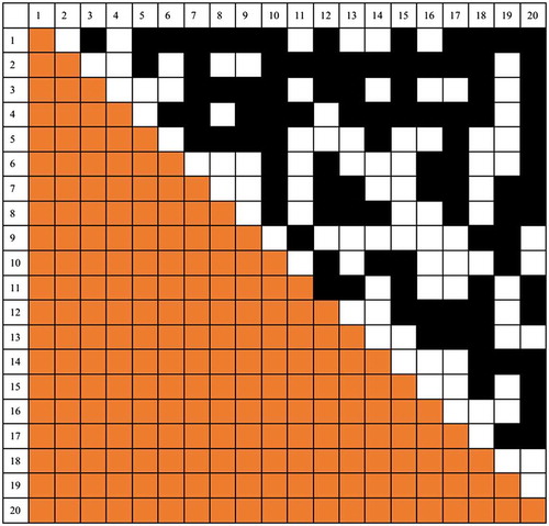
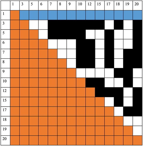
How can we know how many three-event chains are linked to a given event? Let’s start from the first event. We can find the regulation based on each row. For each row in this individual-event pair table, we first delete all columns whose cell value is 0. Second, we delete the corresponding rows in this individual-event pair table. The table below is the result for the first event [row 1]. It means the first event has two-event chain with those remaining events in the first row [colour changed to blue, value is 1]. Thus, the number of three events can be found by only counting the number of black boxes [value is 1], which means these two events are chained together when they both chained with the first event (Figure 2).

Figure 2. Three-event chains that are associated with the first event.

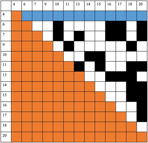
Given another example for the three-event chains that are associated with the fourth event, for each row in this individual-event pair table starting from the fourth event, we first delete all columns whose cell value is 0. Second, we delete the corresponding rows in this individual-event pair table. The table below is the result for the fourth event [row 1]. It means the fourth event has two-event chain with those remaining events in the first row [colour changed to blue, value is 1]. Thus, the number of three events can be found by counting the number of black boxes [value is 1], which means these two events are chained together when they both chained with the fourth event (Figure 3).

Figure 3. Three-event chains that are associated with the fourth event.

For the remaining event chain calculations that have four-event chain or multiple event chains, we found the regulation as: if more than three events are chained together, they will display a regular pattern as in Figure 4 (subset derived from Figure 1).

Figure 4. Regular patterns shown with a higher number of chains.

This means the sum of this subset matrix is n × (n − 1)/2! Thus, we derive the parallel algorithm for multiple event chains that contain more than three events as follows.

For each cell in the 5 × 5 table [i.e. main matrix table]:

1. Since N number of event chains is derived from the result of N − 1 number of event chains, when writing the output of N − 1 number of event chains, a list of unique event IDs associated with this output must be declared and stored. This filter will reduce a significant amount of calculation since those being filtered out have no chance to appear in N number of event chains.

2. Furthermore, when writing the output of N − 1 number of event chains, for each unique event identified in step 1, a list of other unique event IDs associated with this specific event must be declared and stored. This filter will reduce a significant amount of calculations since those being filtered out have no relation to this specific event in the calculations of N number of event chains.

3. Based on the result in step 1, we will create a job queue for task partition in parallel computing. For each unique event, generate a list of N event combination based on the other unique event IDs associated with this specific event derived from step 2, if the number of total events is equal to or greater than N. The list for each unique event will be merged as a single list as the jog queue in order to resolve the unbalanced workload issue in the calculation within such an asymmetric matrix.

4. Based on the result [job queue] in step 3, for each job [i.e. a combination of N event], create a subset matrix from the corresponding individual-event pair table by using the unique IDs listed in the job queue derived in step 3. Calculate the sum of this subset matrix. If the sum equals to n × (n − 1)/2, then this subset of matrix has N event chain, otherwise the result is false.

5. Write the output result by repeating step 1 through 5 until all possible event chains are identified.

3. Result

3.1. Two-event pair calculation over supercomputer Keeneland

Near-repeat calculation for two event pairs over a sample data-set with 32,505 records is implemented on a desktop GPU and supercomputer Keeneland. When the near-repeat calculation is parallelized for calculating two event chains over desktop GPU, while a duplication of the paired values occurs on the GPU side, the duplicated pairs can be eliminated during the integration process on the CPU side. It takes about 48.5 min to complete the entire calculation and simulation processes for a 1000 runs. Furthermore, the near-repeat calculation was implemented on the Keeneland. Through a combination of MPI and GPU programs, we can dispatch the simulation work onto multiple nodes in Keeneland to accelerate the simulation process. MPI programs are developed to handle 100 GPUs on Keeneland to complete 1000 simulations in about 264 s.

For 32,505 events, the total number of two-event pairs is 32,505 × 32,504/2 = 528,271,260, which is exactly the sum of the numbers in the 5 × 5 table (Table 5) derived from the hybrid CUDA and GPU program over Keeneland. Each cell in the table presents the number of the two-event pairs marked by the cell index.

Table 5. Two-event pair calculation result.

902 [0]	19,118 [5]	10,962 [10]	5764 [15]	10,960 [20]
89,430 [1]	10,616,749 [6]	7,096,991 [11]	4,012,736 [16]	7,903,840 [21]
201,122 [2]	24,758,642 [7]	16,575,721 [12]	9,512,489 [17]	18,520,012 [22]
254,539 [3]	31,528,334 [8]	21,104,195 [13]	12,077,044 [18]	23,365,331 [23]
979,689 [4]	121,121,618 [9]	81,166,971 [14]	46,248,867 [19]	91,089,234 [24]

3.2. Multiple-event chain calculation over supercomputer Kraken

While we propose two levels of filters in the prior section, we apply only one filter initially when calculating the three-event chain. That is to say, we use all unique events to generate the combination of possible events as the job queue. Furthermore, we utilize supercomputer Kraken to implement multiple event chain calculation. Supercomputer Kraken is a Cray XT5 system consists of 9,408 compute nodes with 112,896 compute cores, 147 terabytes of memory and 3.3 petabytes storage. Each compute node contains 12 AMD 2.6 GHz Istanbul compute cores and 16 GB memory. Kraken is the first supercomputer in academia that achieves petaflop [10¹⁵ floating point operations]. When we use 120 cores on Kraken to process 100 event sample data, the calculation [1/25 of the main matrix table] on the longest event chain [i.e. 8-event chain] is accomplished in 0.7 s and the result is the same as that from Python program running for 12 h. The same solution was OK with three-event-chain calculation over the 32,505 records. When an average of 2400 processors on Kraken were utilized for each cell in the 5 × 5 table, three-event-chain calculation can be done mostly within about 30 min based on the result of above two-event pairs. If we use a single CPU to do the calculation, it needs 25 × 2400 × 30 = 1,800,000 min or 30,000 h or 1250 days to complete the work.

Table 6 describes the result of the prior work that has successfully completed the calculations of the three event chains. If the number of two-event pairs is greater than 100,000, it will result in a scale of 10¹³ calculations to derive three event chains. It also displays a part of the cells in the 5 × 5 table that have the needs to calculate the potential four-event chains. Since the unique events numbers to be used to calculate four event chains have been identified, the estimated number of calculations reveals that most of the four event chain calculation will be at a scale of 10¹⁶.

Table 6. Three- and Four-event chain calculation result.

ID in 5 × 5 table	Pair number in three event chains	Start time	End time	Time used	Unique events in 4 event chain	Estimated calculations
0	162	01:35:22	02:04:01	0:28:39	170	3.36E+07
1	167,352	02:04:38	02:32:20	0:27:42	23,984	1.38E+16
2	335,568	02:32:49	02:59:42	0:26:53	26,645	2.10E+16
3	284,600	03:07:10	03:35:05	0:27:55	27,871	2.51E+16
4	14,643,984	05:05:54	05:35:14	0:29:20	31,576	4.14E+16
5	107,160	05:36:26	06:03:03	0:26:37	4352	1.49E+13
6	1,897,464,639	06:05:08	06:34:26	0:29:18	32,306	4.54E+16
7	4,147,853,641	06:19:54	06:50:30	0:30:36	32,326	4.55E+16
8	3,612,469,509	06:47:06	07:16:08	0:29:02	32,243	4.50E+16
9	183,759,055,736	06:51:10	07:19:35	0:28:25	32,476	4.63E+16
20	6018	08:35:23	09:01:35	0:26:12	1688	6.05E+10
21	316,239,815	08:49:58	09:18:53	0:28:55	32,466	4.63E+16
22	761,491,797	08:50:47	09:18:21	0:27:34	32,404	4.59E+16
23	633,774,016	08:57:52	09:31:16	0:33:24	32,390	4.59E+16
24	35,091,135,040	08:58:56	09:31:01	0:32:05	32,505	4.65E+16

Several initial results on multiple event chain calculation are accomplished. For the first cell indexed by 0, a maximum number of 9 events can be chained together. 4800 processors were used to complete the task in 130.69 s. Starting from 902 two event pairs, there are 162 three-event chains, 137 four-event chains, 127 five-event chains, 84 six-event chains, 36 seven-event chains, 9 eight-event chains and 1 nine-event chain. For the cell indexed 20 in the above 5 × 5 table, 2400 processors have been used to complete the all event chain calculation in 110.01 s. A maximum number of 4 events can be chained together. Based on 10,960 two-event pairs, there are 6018 three-event chains and 1688 four-event chains.

For the cell indexed five in the above 5 × 5 table, 4800 processors have been used to complete a partial work for the multiple chain calculation in more than 10 h. Starting from 19,118 two-event pairs, there are 107,160 three-event chains, 1,009,866 four-event chains and 9,058,084 five-event chains. There are 1992 unique event IDs that are involved in the calculation for the potential six-event chains. In this case, if only one level of filter is applied, then 10¹⁶ calculations would be involved and beyond our allocation limit on Kraken. For this reason, we plan to apply the second filter to improve the solution. As a result, it is expected that the calculations could be reduced appropriately. Unfortunately Kraken has been decommissioned then we cannot move forward to complete the whole event chain calculation over all data but have to report the latest result and progress over such a challenging research.

4. Conclusion

As a typical example of space–time interaction, near-repeat phenomenon has significant application towards understanding the spatio-temporal patterns of crimes and implementing intelligence-led policing (Ratcliffe, 2016). Given that these concentrations of crime incidents occur in high-crime areas, a series of events would be expected to follow the initiator event. To deal with such time-series spatial data in the context of big data, computation capability is a must. The results are of interest and significance to police and crime prevention specialists to improve policing efficiency and prevent possible follow-up crime incidents through directing police activities at finer spatio-temporal scales. Research on repeat and near-repeat shooting events will provide practical information on gun violence prevention. The analysis will directly guide limited police resources to be prioritized in risky locations during risky time periods once a shooting occurs. Nevertheless, the near-repeat test only determines whether there are more event-pairs in a close proximity of space and time than would be expected on the basis of a random distribution. The challenge is that the linkage beyond paired events is ignored in the near-repeat analysis. Space–time chain is defined as a series of more than three incidents which significantly cluster in space and time. However, it is very computational-intensive to do so. Given the example for a sample data with 30,000 events, near-repeat calculation and simulation can be a petascale (1015) problem to derive all three event chains, or one run of 5-event chain calculation is over exascale (1018). With the aid of high-performance computing, space–time based preventive patrol and social service towards the most at-risk offenders and places can be much more efficiently implemented by utilizing available resources, though more efficient algorithms with parallel solutions have to be further explored.

Recent advances in geocomputation techniques greatly enhance the abilities of social scientists to conduct large-scale data analysis through intensive computation design. Such big data analytics will stimulate the development of new computational models. In turn, these newly developed methods get adopted in real-world practice, forming a positive feedback loop. Enabling such space–time analysis over Cyberinfrastructure is particularly useful for projects such as a Smart City (Batty, 2012), where this positive feedback loop will allow researchers and practitioners to test their models faster and scale them to a larger data-set, therefore producing more policy-relevant results (Wang et al., 2013; Wright & Wang, 2011).

This study has developed a high-performance computing solution to address a challenge in large-scale near-repeat calculation. Follow-up studies on other space–time interaction such as space–time scan statistics, space–time regression or space–time kernel will be illustrated. Setting up permutation of spatio-temporal interaction in parallel is not limited to this case study, because the test of spatial and temporal thresholds is common across space–time analysis, and its permutation is very computing extensive.

Disclosure statement

No potential conflict of interest was reported by the authors.

Data availability statement

The data that support the findings of this study are openly available in Github at https://github.com/xinyueye/TBED1402485.

References

- Andrienko, N., & Andrienko, G. (2013). A visual analytics framework for spatio-temporal analysis and modelling. Data Mining and Knowledge Discovery, 27(1), 55–83.
- Andrienko, G., Andrienko, N., Demsar, U., Dransch, D., Dykes, J., Fabrikant, S. I., … Tominski, C. (2010). Space, time and visual analytics. International Journal of Geographical Information Science, 24(10), 1577–1600.10.1080/13658816.2010.508043
- Anselin, L. (2012). From spacestat to cyberGIS twenty years of spatial data analysis software. International Regional Science Review, 35(2), 131–157.10.1177/0160017612438615
- Batty, M. (2012). Smart cities, big data. Environment and Planning-Part B, 39(2), 191–193.10.1068/b3902ed
- Emeno, K. (2014). Space-time clustering and prospective hot-spotting of canadian crime (Doctoral dissertation). Carleton University).
- Goodchild, M. F. (2009). Geographic information systems and science: Today and tomorrow. Annals of GIS, 15(1), 3–9.10.1080/19475680903250715
- Goodchild, M. F., & Janelle, D. G. (2004). Spatially integrated social science. New York, NY: Oxford University Press.
- Gu, Y., Wang, Q., & Yi, G. (2017). Stationary patterns and their selection mechanism of Urban crime models with heterogeneous near–repeat victimization effect. European Journal of Applied Mathematics, 28(1), 141–178.
- Henriksen, C. B., Mattick, K. L., & Fisher, B. S. (2016). Repeat victimization. The encyclopedia of crime & punishment. doi:10.1002/9781118519639.wbecpx036
- Johnson, S. D., Summers, L., & Pease, K. (2009). Offender as forager? A direct test of the boost account of victimization. Journal of Quantitative Criminology, 25(2), 181–200.10.1007/s10940-008-9060-8
- Knox, E., & Bartlett, M. (1964). The detection of space-time interactions. Applied Statistics, 13, 25–30.10.2307/2985220
- Ratcliffe, J. H. (2016). Intelligence-led policing. Abingdon: Routledge.
- Ratcliffe, J. H., & Rengert, G. F. (2008). Near-repeat patterns in Philadelphia shooting events. Security Journal, 21(1–2), 58–76.10.1057/palgrave.sj.8350068
- Shi, X., Lai, C., Huang, M., & You, H. (2014). Geocomputation over the emerging heterogeneous computing infrastructure. Transactions in GIS. doi:10.1111/tgis.12108
- Townsley, M. (2007). Near repeat Burglary chains: Describing the physical and network properties of a network of close Burglary Pairs. Presentation at the International Crime Hot Spots: Behavioural, Computational and Mathematical Models Conference, Institute for Pure & Applied Mathematics conference UCLA, February, Los Angeles, USA.
- Townsley, M., Homel, R., & Chaseling, J. (2000). Repeat Burglary victimisation: Spatial and temporal patterns. Australian & New Zealand Journal of Criminology, 33(1), 37–63.10.1177/000486580003300104
- Vetter, J. S., Glassbrook, R., Dongarra, J., Schwan, K., Loftis, B., McNally, S., ... Yalamanchili, S. (2011). Keeneland: Bringing heterogeneous gpu computing to the computational science community. Computing in Science and Engineering, 13(5), 90–95.10.1109/MCSE.2011.83
- Wang, S., Anselin, L., Bhaduri, B., Crosby, C., Goodchild, M. F., Liu, Y., & Nyerges, T. L. (2013). CyberGIS software: A synthetic review and integration roadmap. International Journal of Geographical Information Science, 27(11), 2122–2145.10.1080/13658816.2013.776049
- Wells, W., Wu, L., & Ye, X. (2011). Patterns of near-repeat gun assaults in Houston. Journal of Research in Crime and Delinquency, 49, 186–212.
- Wright, D. J., & Wang, S. (2011). The emergence of spatial cyberinfrastructure. Proceedings of the National Academy of Sciences, 108(14), 5488–5491.10.1073/pnas.1103051108
- Ye, X., & Liu, L. (2012). Special issue on spatial crime analysis and modeling. Annals of GIS, 18(3), 157–241.10.1080/19475683.2012.693342
- Ye, X., & Rey, S. (2013). A framework for exploratory space-time analysis of economic data. The Annals of Regional Science, 50(1), 315–339.10.1007/s00168-011-0470-4
- Ye, X., & Shi, X. (2013). Pursuing spatiotemporally integrated social science over cyberinfrastructure. In Shi, X., Kindratenko, V., & Yang, C. (eds.) Modern accelerator technologies for GIScience. pp. 215–226. Springer.
- Zeoli, A. M., Pizarro, J. M., Grady, S. C., & Melde, C. (2014). Homicide as infectious disease: Using public health methods to investigate the diffusion of homicide. Justice Quarterly, 31(3), 609–632.10.1080/07418825.2012.732100