Exploiting big earth data from space – first experiences with the timescan processing chain

Abstract

The European Sentinel missions and the latest generation of the United States Landsat satellites provide new opportunities for global environmental monitoring. They acquire imagery at spatial resolutions between 10 and 60 m in a temporal and spatial coverage that could before only be realized on the basis of lower resolution Earth observation data ($>$250 m). However, images gathered by these modern missions rapidly add up to data volume that can no longer be handled with standard work stations and software solutions. Hence, this contribution introduces the TimeScan concept which combines pre-existing tools to an exemplary modular pipeline for the flexible and scalable processing of massive image data collections on a variety of (private or public) computing clusters. The TimeScan framework covers solutions for data access to arbitrary mission archives (with different data provisioning policies) and data ingestion into a processing environment (EO2Data module), mission specific pre-processing of multi-temporal data collections (Data2TimeS module), and the generation of a final TimeScan baseline product (TimeS2Stats module) providing a spectrally and temporally harmonized representation of the observed surfaces. Technically, a TimeScan layer aggregates the information content of hundreds or thousands of single images available for the area and time period of interest (i.e. up to hundreds of TBs or even PBs of data) into a higher level product with significantly reduced volume. In first test, the TimeScan pipeline has been used to process a global coverage of 452,799 multispectral Landsat–8 scenes acquired from 2013 to 2015, a global data-set of 25,550 Envisat ASAR radar images collected 2010–2012, and regional Sentinel–1 and Sentinel–2 collections of $\sim$1500 images acquired from 2014 to 2016. The resulting TimeScan products have already been successfully used in various studies related to the large-scale monitoring of environmental processes and their temporal dynamics.

Keywords:

• Earth observation
• sentinel
• landsat
• mass data
• high performance processing
• information and communication technology
• automation

1. Introduction

Assessing and monitoring the state and change of the Earth surface is a key requirement for a variety of research activities focusing on topics such as climate change, human impact, biodiversity, security or geohazards. This is also reflected by several related initiatives and programmes, e.g. by the Group on Earth Observation (GEO) (Cao, Strohmeier, Mjwara & Sullivan, 2016) or the European Copernicus programme (European Commission, 2013). The launch of the new fleet of Sentinel Earth observation (EO) satellites by the European Space Agency (ESA) has considerably enhanced the opportunities to monitor the Earth system (Wulder & Coops, 2014). In particular, Sentinel–1 (synthetic aperture radar – SAR), Sentinel–2 (medium resolution multispectral) and Sentinel–3 (low resolution, multi-instrument) are designed to support operational geoinformation services, especially those of the European Copernicus programme (European Space Agency, 2017c). In its final constellation, which is expected to be completed by summer 2018, each Sentinel–1/–2/–3 mission will include two satellites in order to assure high revisiting times and a fast coverage of large areas.

The exponentially growing availability of open and free EO satellite data combined with the increasing spatial and temporal resolution of modern satellite missions is expected to significantly improve existing remote sensing applications, including land use/land cover (LULC) and vegetation mapping (Congalton, Gu, Yadav, Thenkabail & Ozdogan, 2014; Fritz & See, 2008; Hansen et al., 2013; Xie, Sha & Yu, 2008), urban analyses (Esch et al., 2013; Potere et al., 2009) as well as marine (Blondeau-Patissier, Gower, Dekker, Phinn & Brando, 2014) and atmospheric monitoring (Hoff & Christopher, 2009; Martin, 2008). Furthermore, a broad spectrum of synergetic applications will be fostered, especially related to the monitoring of effects linked to climate change (Jung, Henkel, Herold & Churkina, 2006) and vegetation dynamics (Eamus, Huete & Yu, 2016) or associated processes like vegetation carbon and energy modelling (Tum, Zeidler, Günther & Esch, 2016). The Sentinels, but also other “big data”? missions such as the Landsat programme (United States Geological Survey, 2017a), can therefore be expected to herald a new era with respect to the promotion of innovation in the scientific and commercial technology and service sector based on the use of EO data.

Although the growing availability of EO data offers an emerging spectrum of new opportunities, this development at the same time challenges established concepts of how data are delivered from the mission ground segments to the local environment of individual expert users. Missions like the European Envisat, the US Moderate resolution imaging spectroradiometer (MODIS) and Advanced very high resolution radiometer (AVHRR) were designed to operationally monitor the Earth surface at low resolution ($\sim$ 300–1000 m), resulting in a data collection rate of $\sim$ 30–50 GB per day. At the same time, commercial missions with high spatial resolution (HR, $\sim$ 10–60 m) such as the US Landsat programme, the French Satellite Pour l’Observation de la Terre (SPOT) or the Indian Ressourcesat (IRS) systematically collected data on global scale. The opening of the Landsat archive represented a first step change in the EO sector (Woodcock et al., 2008) – in particular since the Landsat programme provides the longest continuous record of HR EO satellite imagery, covering a time span from the 1970s until today and currently growing at a rate of $\sim$ 0.5 TB per day (Baumann et al., 2016). A comprehensive review by (Wulder & Coops, 2014) identifies a broad spectrum of thematic applications directly benefiting from the availability of the open and free Landsat data archive, in particular the mapping and monitoring of vegetation, phenology and agricultural activity, built environments, water, wetlands and coastal zones, as well as polar and alpine regions.

At the same time, an increasing amount of highly automated data processing and analysis approaches have been developed, for instance, to provide comprehensive Landsat data collections in form of mosaics or weekly, monthly, seasonal or yearly image composites (Roy et al., 2010; White et al., 2014). The Sentinel–1/–2/–3 missions are expected to collect about 20 TB of data per day, which is an order of magnitude higher compared to the established systems (Rosengren, 2014). The Sentinel missions and the related Copernicus programme can therefore be expected to initiate a next step change by making EO data enter the big data era (Wagner, 2015).

However, the current concept of delivering data from the mission ground segments to each single user who then performs an individual processing and analysis in the local private working environment comes along with significant limitations when considering the absolute mass of data which is potentially available. First, immense amounts of data have to be transferred from the mission ground segments to thousands of users within a reasonable time. Secondly, the user must be able to effectively store, manage, process and analyze the mass data volumes – a task that increasingly challenges the capabilities of processing environments composed of individual personal workstations. Hence, the established processing and analysis concepts need to be revised. Ideally, the specific processing functionalities and toolboxes of the users – or required by the users – should be moved to and deployed at a (remote) entity where both mission archives and an adequate processing infrastructure are effectively linked with each other in one single system. Such an approach would significantly increase the efficiency of processing and analysis (e.g. in terms of time, scalability and therewith costs, etc.) and, at the same time, the mass transfer and duplication of data is avoided whereas classical barriers such as hardware and software requirements are given over to specialized entities.

Here, modern information and communication technology (ICT) such as hosted computing platforms and services (e.g. cloud computing, grid computing) offer a very promising perspective. A well-known example is the Google Earth Engine (Gorelick et al., 2017), which provides the possibility to develop algorithms in an environment which is directly linked to mass EO data collections (e.g. from Landsat, Sentinel–1, Sentinel–2, MODIS) and which has already been tested and successfully used for a variety of EO-based thematic analyses (Hansen et al., 2013; Trianni, Angiuli, Lisini & Gamba, 2014; Pekel, Cottam, Gorelick & Belward, 2016). Another option is provided by Amazon Web Services (AWS) where all Sentinel–2 scenes are made available in a high level processing environment (Amazon Web Services, 2017). ESA has launched the Thematic Exploitation Platform (TEP) initiative capitalizing on ground segment capabilities and ICT to maximize the exploitation of EO data from past and future EO missions for dedicated application areas such as coastal, forest, geohazard, hydrology and urban (European Space Agency, 2017h).

The facts and trends previously described highlight that the ability to utilize scalable high performance computing platforms with direct access to complete mission archives will become a key factor in future to assure a fully effective and efficient exploitation of modern EO missions by a broad spectrum of (non-expert) users, which do not have direct or high performance access to data archives and/or powerful processing infrastructures. At the same time, it is of key importance that the users will not be trapped by any vendor lock-in in order to fully exploit the big data perspective of modern EO missions. Hence, the design of the TimeScan approach aims at demonstrating an exemplary way of how existing tools can be used and combined by a broad spectrum of users in a way that:

• supports the processing of massive image data collections,

• can be flexibly adapted to different missions and data provisioning models,

• can be deployed at any standard hosted or private processing infrastructure (high performance platforms for distributed computing, but also local workstations), and

• transfers a massive collection of single EO images into a higher processing level product with significantly reduced volume that still reflects key spatial and spectral characteristics such as they are required for thematic analyses and value adding services.

2. The timescan processing pipeline – a set of functions to exploit massive Earth observation data collections

TimeScan comprises two things: A convention how to processes time series data-sets and software tools implemented according to it. The convention serves as a blueprint for the single components and makes sure that they are able to interact in different processing pipelines. It does not constitute a framework with an API but defines the way data are structured, accessed and processed. This approach was deliberately chosen to be able to use a wide range of computing clusters. If the computing environement provides an orchestration tool or workflow manager, then the TimeScan pipelines can easily be incorporated into it. However, if for computing platforms without a resource management the TimeScan pipelines can easily be scripted and executed in a stand-alone manner.

A TimeScan processing pipeline consists of three basic functional components that are sequentially applied to form a coherent processing chain: (i) the EO2Data module organizing data access and ingestion; (ii) the Data2TimeS module conducting a specific pre-processing and data preparation of multitemporal EO image collections and (iii) the final TimeS2Stats module which represents a generic software aggregating all available data for a defined area and time span of interest into the higher processing level TimeScan product.

In general, the basic TimeScan modules and underlying tools and functionalities are as far as possible implemented in form of self-contained, hardware-independent solutions which can be controlled and orchestrated by any higher level workflow management. This design facilitates a flexible and scalable deployment in any prevalent computing environment – a prerequisite for concepts that finally aim at bringing the user (represented by an algorithm or tool) to the data (meaning an infrastructure where mission archives and high-performance processing are directly coupled).

To develop a better understanding of the possibilities and constraints arising from this concept, the TimeScan implementations used for this study cover a variety of scenarios with different representative constellations for the processing environment, EO missions and data access models. The testbed of distributed computing infrastructures included a Calvalus (Fomferra, Böttcher, Zühlke, Brockmann & Kwiatkowska, 2012) cluster based on Apache Hadoop (Hadoop, 2016), an Apache Mesos-orchestrated cloud of virtual machines and a High Performance Cluster. Considering the data provisioning scenarios, different access modes based on push or pull mechanisms were tested on the basis of the Landsat, Envisat and Sentinel missions. A schematic view of the TimeScan processing pipeline is provided in Figure 1.

Figure 1. Schematic view of the modular and adaptive TimeScan processing chain used to test options of effectively linking users (meaning their software, toolboxes, applications), processing entities and mission archives as a basis to fully exploit the “big data” perspective of modern EO missions).

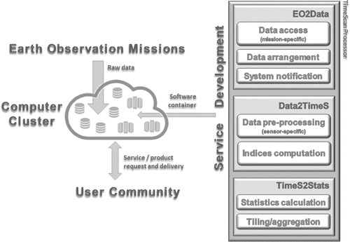
2.1. Data access and retrieval – the EO2Data module

The EO2Data module is optional and only required in case a processing environment does not yet provide local access to the required EO data. Its main purpose is to obtain imagery from different archives and store it in a predefined file structure on a cluster or cloud. Additionally, some tools of the EO2Data module are also responsible for data arrangement and system notification. In general, the data provisioning tools of EO2Data are able to deal with the two common data exchange scenarios: data pull and data push. Both modes depend on suitable protocols and services and each scenario has its merits. In the first case, a data-set is downloaded from a server and saved locally for long-term (mirroring) or temporary (caching) storage. In the second (and increasingly more popular) case, a data-set is sent from a server to a local destination. This can be considered as a subscription or event-driven service which is particularly suited for cases when new EO data or results of a remote processing are actively pushed to the customer or another facility where further processing or analyses are triggered as soon as new data arrive. This scenario avoids constant polling of the producer’s archives and also eliminates notifications of the producer regarding the processing status.

Considering the pull scenario, EO2Data includes a download tool that provides options to select parameters such as the data provider/EO mission or the time and area of interest. The tool is accessed from the command line and provides a uniform syntax. Therefore, it hides individual characteristics of each EO data provider or mission archive using a dedicated adapter that either scrapes the graphical user interface (GUI) or uses an application programming interface (API) offered by the provider / archive. After a specific request is executed the software checks if the data are already present at the target facility and, if not, it retrieves it. Multiple instances of the software can be run in parallel to get data from different sources at the same time or increase the download rate and volume. The tool can be triggered periodically using any scheduler (e.g. cronjob, Apache Mesos) and can therewith be used as a data harvester, which continuously searches for new data and keeps a given EO data collection up to date.

Tools for handling push scenarios usually work in two modes. They check a pick-up-point for new data arrivals and either transfer the data to the desired location in the processing facility or they generate a notification which is sent to an event processing engine. The latter is suited for cases when the data need some form of modification prior to processing (e.g. unpacking of archives, format conversion, meta-data enrichment, etc.).

The different tools available in the EO2Data module can trigger routines or can be part of workflows by interfacing with the software infrastructure of a processing cluster. As mentioned above, they can be called from the command line; accordingly, it is rather simple to bundle a set of tools in a Docker container (Hykes, 2013) that fulfilling a given purpose. The container can then be deployed on a processing platform where it represents a micro-service. Working with containers allows managing and orchestrating them in high-availability and highly parallelized cluster systems by running multiple instances.

In the context of this study, the Envisat ASAR and Sentinel–1 processing included a push scenario with the ASAR data being pre-processed at ESA’s grid processing on demand platform G-POD (European Space Agency, 2017e) before the results were then pushed to DLR’s processing facility as input to the data preparation tools of the Data2TimeS instance (more details provided in Section 2.2). Regarding Sentinel–1, the raw data were pushed from ESA’s processing and archiving centre (PAC) to DLR’s processing facility for the TimeScan processing. For Landsat and Sentinel–2, the EO2Data harvesting tool was applied. In this data pull approach, the Landsat imagery was simultaneously downloaded from archives at USGS, ESA and Google to a HPC cluster where it was stored temporary (caching) until the subsequent processing with Data2TimeS and TimeS2Stats were performed. In the case of Sentinel–2, the harvesting tool was employed for data download from the Copernicus Open Access Hub (European Space Agency, 2017b) to a Calvalus Cluster.

2.2. Data pre-processing and preparation – the Data2TimeS module

Once the required data are gathered, they need to be properly arranged for the actual processing tasks. This is accomplished by employing the Data2TimeS module, which includes both pre-processing (i.e. upgrade from low to high level products) and (optional) "data-preparation" tools.

In general, pre-processing tools are often mission-specific and have to be tailored for special purposes. Here, the concept of pre-processing significantly varies between optical and radar data (due to the fundamental differences in their imaging principles) but also among specific sensors. Nevertheless, classical pre-processing tasks of low-level EO products (e.g. radar terrain correction or optical atmospheric correction) are normally performed using largely employed software (i.e. ATCOR, SNAP, etc.). Therefore, Data2TimeS tools often just represent a wrapper around one of these well-established packages.

The goal of the data-preparation tools is to convert the pre-processed data into a standardized database to be given as input to the final TimeS2Stats module. This basically corresponds to extract features ideally requiring relatively few resources both in terms of computational load and time bearing key information to effectively support the given application of interest as, for instance, thematic land cover classification. In this context, a simple but effective solution in the case of multispectral imagery is the computation of normalized difference indices, which also allows compensating for atmospheric effects like mist or haze (generally not properly removed even using advanced atmospheric correction software). Instead, for radar data texture features from the grey level co-occurrence matrix (GLCM) or Kennaugh elements in the case of multi-polarization imagery represent potential effective solutions.

In this work, we took into consideration optical Landsat and Sentinel-2, as well as radar Sentinel-1 and Envisat ASAR imagery.

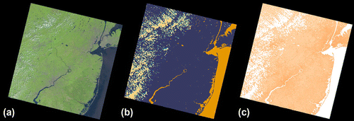
For Landsat data, the Data2TimeS workflow starts with the calibration of the original imagery (i.e. the conversion from digital numbers to at sensor radiance) available at 30m spatial resolution. Next, the FMask software (Zhu & Woodcock, 2012) is applied to all available input scenes for computing the corresponding cloud, shadow and water mask. Here, a valuable option to avoid massive processing is to use USGS’s Earth Resources Observation and Science (EROS) Center Science Processing Architecture (ESPA) On Demand Interface. In particular, the ESPA interface allows to directly obtain the FMask for a given list of input scenes provided in a text file (United States Geological Survey, 2017b). In the framework of this study, six indices have been then extracted (see Figure 2), namely the Normalized Difference Vegetation Index (NDVI), the Normalized Difference Built-up Index (NDBI), the Modified Normalized Difference Water Index (MNDWI), the Normalized Difference Middle Infrared index (NDMIR), the Normalized Difference Red Blue index (NDRB) and the Normalized Difference Green Blue index (NDGB) (see Table  1).

For Sentinel–2 data, the Data2TimeS module has been implemented as a processing graph in the ESA SNAP Toolbox (European Space Agency, 2017d). Specifically, a reader interprets the multi-resolution input, a resampling operator rescales all bands to 20m spatial resolution, the Sentinel2.Idepix operator generates a flag band with cloud identification, whereas BandMaths operators compute the same indices adopted in the case of Landsat data (see Table 1).

Table 1. List of calculated spectral indices.

Spectral index	Equation landsat	Equation Sentinel–2	Citation
NDVI	(NIR–Red)/(NIR+Red)	(B8A–B4)/(B8A+B4)	*Rouse1973
NDBI	(MIR1–NIR)/(MIR1+NIR)	(B11–B8A)/(B11+B8A)	*Zha2003
MNDWI	(Green–NIR)/(Green+NIR)	(B3–B8A)/(B3+B8A)	Xu (2006)
NDMIR	(MIR1–MIR2)/(MIR1+MIR2)	(B11–B12)/(B11+B12)	*Lu2004
NDRB	(Red–Blue)/(Red+Blue)	(B4–B2)/(B4+B2)	Zhou et al. (2014)
NDGB	(Green–Blue)/(Green+Blue)	(B3–B2)/(B3+B2)	Zhou et al. (2014)

When analyzing optical data, Data2TimeS tools might also be used in concert with the CATENA pre-processing framework (Krauß, 2014). CATENA supports the common pre-processing steps of most of the established HR satellite missions (i.e. Landsat, SPOT, IRS, RapidEye), such as calibration, orthorectification and atmospheric correction. In the context of this work, CATENA has been packed in form of a Docker container and could then be used optionally for the pre-processing part, whereas the data preparation was done with dedicated Data2TimeS tools containers.

Concerning Sentinel–1 data, Level–1 Ground Range Detected (GRD) imagery acquired at high resolution (HR) in Interferometric Wide Swath mode (IW) with VV polarization (European Space Agency, 2013) have been taken into account and a dedicated pre-processing chain has been implemented by means of the Sentinel–1 toolbox as part of ESA SNAP (European Space Agency, 2017d). This includes orbit correction (using precise orbit information), thermal noise removal (for excluding dark strips with invalid data near the scene edges), radiometric calibration and Range Doppler terrain correction using the SRTM 30m DEM (United States Geological Survey, 2017b). Final pre-processed data are derived at 10m spatial resolution.

As regards Envisat ASAR, Wide Swath Mode (WSM) data (European Space Agency, 2017f) acquired with VV polarization have been used and, similarly to Sentinel–1, their pre-processing was also performed by means of the SNAP Toolbox. Specifically, this included orbit correction, radiometric calibration and SAR-simulated terrain correction (based on extensive empirical analysis, the terrain correction always proved more effective than Range Doppler correction for this specific type of data). For the latter, the SRTM 30m DEM for latitudes comprised between –60 ${}^{\circ }$ and +60 ${}^{\circ }$ and elsewhere the ASTER GDEM (National Aeronautics and Space Administration, 2017) were used. Final pre-processed data are derived at 75m spatial resolution.

Both for Sentinel-1 and ASAR data, no data-preparation tool has been applied after the pre-processing; hence, only the corresponding backscattering coefficient time series have been given as input to the TimeS2Stats module.

Figure 2. Example of the Data2TimeS processing workflow applied to multispectral data including calibration and atmospheric correction (a), masking of clouds (light orange), cloud shadows (light blue), and water (orange) (b), and the calculation of indices for all unmasked pixels of the input image (c).

2.3. Generation of higher processing level baseline product – the TimeS2Stats module

The overall objective of TimeS2Stats is the transformation of the large database generated by the Data2TimeS module into a new data-set of consistently smaller size (hence sensibly easier to handle) which properly combines the information of the whole input time series. To this purpose, an effective solution proved the computation for all Data2TimeS output features of key temporal statistics including minimum, maximum, mean, standard deviation and mean slope (i.e. the average of the absolute difference between consecutive items of the series) calculated for each pixel in the given area of interest over time. Along with these, also the number of available input items for each pixel is extracted (which can be used as quality parameter for assessing the robustness of the statistics). Furthermore, when a specific mask is provided for the entire input series, then the temporal statistics are solely computed over the corresponding valid items (e.g. in the case of optical imagery if a cloud/cloud-shadow mask is available, statistics are calculated for each pixel only over cloud-free acquisitions).

In this context, it is worth noting that the TimeS2Stats module can be independently applied both to any optical- or radar-based input features without the need for specific adjustments.

In our experimental framework, the final Landsat and Sentinel-2 TimeScan data-sets include 31 features (i.e. five temporal features for each of the six extracted normalized difference indices plus the number of cloud-free acquisitions per pixel). Instead, in the case of Sentinel-1 and Envisat ASAR, the corresponding TimeScan products are composed of six features (i.e. five temporal statistics for the backscattering coefficient plus the number of available acquisitions per pixel).

To effectively deal with large geographical areas, the final output can optionally be stored in form of tiles with an arbitrary size. In particular, when performing national to global analyses a tiling of 1 ${}^{\circ }$ x 1 ${}^{\circ }$ geographical lat/lon proved in our tests being a good compromise between file size and number of resulting tiles. At the same time, this also allows an efficient calculation on a distributed computing cluster since the processing of individual tiles is independent from all others.

The implementation of the TimeS2Stats on a Calvalus cluster is different from other platforms as it employs map reduce for concurrent aggregation. The map steps – one per input file – apply the Data2TimeS function concurrently to the input time series. All intermediate results are sorted in memory, streamed and merged directly to the reducers without storing them. The reduce steps – one per target tile – concurrently aggregate the intermediate products and apply the TimeS2Stats module. Calvalus controls the re-projection to a common raster and the sorting and streaming of the outputs of map steps for the concurrent reduce steps.

3. First results of large-scale TimeScan applications

In a first test and demonstration phase, different TimeScan implementations deployed at three computer clusters (i.e. cloud, Calvalus cluster, HPC) were used to process a comprehensive EO data collection including both multispectral and radar imagery. This included the generation of two global layers based on Landsat–8 (TimeScan–Landsat–2015) and ASAR WSM (TimeScan–ASAR–2012) imagery, respectively, along with two layers covering Germany derived from Sentinel–1 (TimeScan–Sentinel–1–2015) and Sentinel–2 (TimeScan–Sentinel–2–2015) data, respectively.

The TimeScan–Landsat–2015 product (Figure 3) was derived from 452,799 multispectral Landsat–8 images acquired from April 2013 to November 2015 and has a size of 25 TB ($\sim$ 20 times smaller than the total size of the original input data which sums up to about 500 TB). Considering all intermediate products, a total of 1.5 PB was handled during the processing which required a total of approximately 120,000 core hours. These numbers underline that such a data-set could hardly be generated by users that just have access to standard computing environments or even only to private workstations. In Figure 3(a), the RGB colour composite obtained combining the temporal mean NDBI (red channel), NDVI (green channel) and MNDWI (blue channel) is given. As one can immediately notice, despite the employment of a massive amount of scenes the map appears even at this scale extremely homogeneous, without any considerable striping effect as compared instead to the number of cloud-free acquisitions per pixel reported in Figure 3(b). Here, in the large part of the world more than 10 items were available and only in remote northern regions or in tropical areas this value dropped to lower than five (which might partially affect the robustness of the corresponding temporal statistics).

Figure 3. Global TimeScan–Landsat–2015 layer (a) visualized as false colour composite with the temporal mean of the built-up index (NDBI) in red, the vegetation index (NDVI) in green and the water index (MNDWI) in blue, and TimeScan band 31 indicating the total number of valid acquisitions per pixel for the product generation.

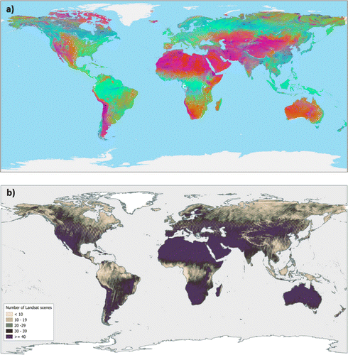
Figure 4. Comparison of single date Landsat–8 scenes (a, d) with corresponding pseudo colour RGB images of the outcome of the TimeScan Data2Stats module (b, c, e, f) which are derived on the basis of all available Landsat–8 images in 2013–2015. The single scenes cover the visible bands whereas the TimeScan layers are composed of the temporal maximum of NDBI, temporal maximum of NDVI, and mean of MNDWI (b, e) and maximum NDVI, mean NDVI and minimum NDVI (f), respectively.

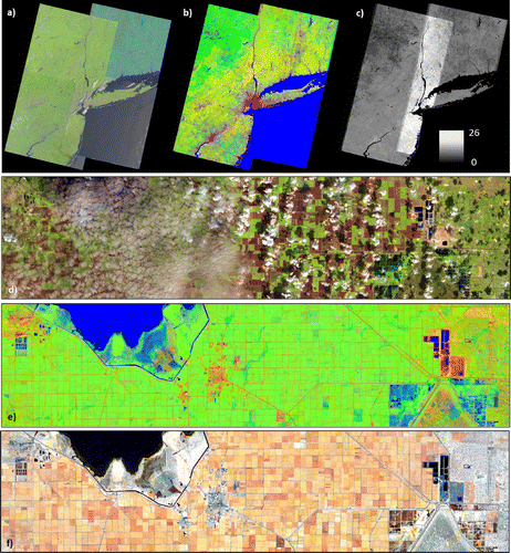
To better appreciate the capabilities offered by the TimeScan–Landsat–2015 data-set, local examples are provided in (Figure 4).

Figure 4(a–c) refer to a region including the city of New York (USA) which is covered by four Landsat path-row combinations according to the Worldwide Reference System-2 (WRS-2). Specifically, Figure 4(a) depicts the mosaic obtained by combining for each path-row combination the corresponding scene with lowest cloud-coverage among all those collected between April 2013 and November 2015. Here, it is still evident the presence of clouds, as well as the heterogeneity among the four selected scenes which have been acquired at different times in the year corresponding to as many different phenological states of the vegetation. Figure 4(b) shows instead an RGB combination of the TimeScan–Landsat–2015 obtained combining the temporal maximum NDBI (red channel), temporal maximum NDVI (green channel) and temporal mean MNDWI (blue channel) which appears extremely homogeneous despite the consistent difference in the number of cloud-free acquisition per pixel (Figure 4(c)). Furthermore, it is also clear how different land cover types tend to be associated with specific colours, thus making their categorization a relatively simple task.

Figure 4(d–f) refer to a region located in southern Florida including part of Lake Okeechobee in the upper left, as well as the outskirt of the West Palm Beach urban area on the right. Figure 4(d) shows the corresponding portion of the Landsat–8 scene acquired on 2nd January 2014 which has been employed in the generation of the TimeScan–Landsat–2015 and is characterized by a consistent presence of clouds. Nevertheless, no discontinuities appear in the final TimeScan layer as evident from the two different RGB compositions reported in Figure 4(e) and Figure 4(f), respectively. In Figure 4(e), the same bands used as in Figure 4(b) have been employed, hence resulting in: (i) human settlements and extraction sites being associated with red tones due to the relative dominance of the temporal maximum NDBI; (ii) highly vegetated areas as forests and permanent crops appearing in green tones due to the high temporal maximum NDVI; and (iii) water bodies and wetlands being depicted in blue tones due to the relatively high and stable MNDWI over time. This combination has also been used in Figure 5(a), where the subset of the TimeScan–Landsat–2015 layer for Germany is shown.

Instead, Figure 4(f) is obtained combining the temporal maximum, minimum and mean NDVI. In this framework, agricultural areas are associated with different yellow/orange tones, whereas water bodies and urban areas appear in black and grey colours, respectively.

The TimeScan–Sentinel–2–2015 data-set over Germany has been derived from 9,692 Sentinel–2 L1C granules acquired between August 2015 and November 2016 (European Space Agency, 2017f). Thereby, the original input data volume of 3.1 TB was reduced to 121 GB (hence with a compression factor $\sim$ 25). Figure 5(b) reports the RGB composition obtained combining the temporal maximum NDBI (red channel), temporal maximum NDVI (green channel) and temporal mean MNDWI (blue channel), resulting in an overall appearance quite comparable to that of the TimeScan–Landsat–2015 in Figure 5(a).

The TimeScan–ASAR–2012 data-set was generated from 25,550 Envisat ASAR WSM scenes acquired between 2010 and 2012 (European Space Agency, 2017a). The available imagery does not allow to form a complete and consistent global coverage due to the non-systematic worldwide acquisition plan of the ASAR sensor; however, due to its all-weather capabilities, where data have been collected the number of available scenes is usually rather high (>30). The total size of input data was 8.4 TB, in contrast to the resulting TimeScan layer whose volume is only 574 GB. In the pseudo colour RGB representation of the TimeScan–ASAR–2012 subset for Germany illustrated in Figure 5(c) the red, green and blue channels are associated with the temporal mean, minimum and maximum backscattering, respectively. Thereby, urban conglomerations appear as bright white regions due to their constantly high values over time. Water bodies deflect a large portion of the oblique radar beams from the satellite and are hence associated with dark tones. Vegetated regions can be distinguished due to their relatively high temporal minimum backscattering resulting in green tones. Finally, land cover types whose characteristics change considerably during the investigated time frame (e.g. crop acreage) appear in lilac-brownish shades.

Figure 5. Comparison of TimeScan–Landsat–2015 (a), TimeScan–Sentinel–2–2015 (b), TimeScan–ASAR–2012 (c) and TimeScan–Sentinel–1–2015 (d) for the area of Germany.

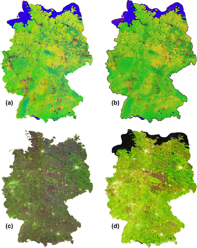
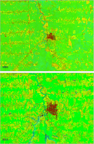
Figure 6. TimeScan–Landsat products of the region around the Brasilian city of Ariquemes, derived from data collected in 1984–1985 and 2013–2015.

The TimeScan–Sentinel–1–2015 data-set was derived from 1,444 IW-GRDH scenes acquired in in VV polarization (European Space Agency, 2013) between October 2014 and June 2016. The total volume of the input data is about 2.35 TB, whereas the corresponding TimeScan layer has a volume of 102 GB. Also in this case, the pseudo colour image reported in Figure 5(d) is obtained combining the mean (red channel), minimum (green channel) and maximum (blue channel) backscattering over time, hence exhibiting a behaviour similar to that of the TimeScan ASAR–2012 layer for the same region: settlements stick out as bright white areas, woodland and intense vegetation appears in greenish tones, whereas temporally variable land cover types such as agricultural regions are associated with purple and brownish colours.

Finally, to give a general idea of the high potential of TimeScan products for supporting change detection tasks, we computed for a test area around the Brasilian city of Ariquemes the corresponding TimeScan–Landsat–5–1985 product (derived from 21 Landsat–5 scenes acquired in 1984–1985). Here, yet when comparing the RGB colour composition obtained combining the temporal maximum NDBI (red channel), temporal maximum NDVI (green channel) and temporal mean MNDWI (blue channel) against that of the corresponding TimeScan–Landsat–8–2015 reported in Figure 6 it is possible to immediately notice the changed occurred in the considered region. In particular, it is evident the expansion of built-up and agricultural areas (associated with red and yellow/orange tones, respectively) and the corresponding decrease in vegetation areas (associated with green tones) due to intense logging activities. At the same time, an increased amount of small water bodies (mainly dammed lakes) is associated with the appearance of pixels in blue colours at the recent time.

4. Conclusions and outlook

To test the capability of exploiting the information content of massive image collections, TimeScan implementations were exemplary deployed for Landsat, Envisat ASAR, Sentinel–1 and Sentinel–2 data at different high performance processing infrastructures.

From a technical view point, the experiments demonstrated the suitability of the TimeScan approach to be deployed on a variety of standard hosted or private platforms for distributed computing. Moreover, TimeScan versions were successfully installed at Windows PCs and other local workstations. In the last years, developments in the remote sensing and IT communities drastically changed the scope and capability of EO data processing. It is now possible to host entire data-sets of one or more missions at one location and repeatedly analyze them according to given requirements. Large processing clusters can be afforded by organizations or even rented commercially by users on demand. In order to be as flexible and independent as possible from the underlying IT infrastructure, we developed a processing pipeline that can be operated in a wide range of processing environments, settings and application scenarios. In this way, it is possible to deploy the software as close as possible to the data in order to minimize I/O operations (software-to-data paradigm).

One important aspect of this concept in TimeScan is to split related tasks into three different modules (EO2Data, Data2TimeS, TimeS2Stats), which share many conventions and, wherever possible, a common code base, while designing independent tools for each task that can be run from the command line. This approach follows the Unix philosophy, where tools are designed to perform a very specific job with high efficiency and the output of one tool can be the input to another (McIlroy, Pinson & Tague, 1978). Another decision in the TimeScan design was to restrict the dependencies to few "de facto" standard libraries for spatial (e.g. GDAL) and statistical purposes and implement the processing intensive tasks in a lower level language. Finally, compiler platforms of low level tools also included Cygwin to be able to use Windows PCs, especially for testing or small-scale desktop processing.

Following this concept, the creation and orchestration of workflows is left to the infrastructure of the specific platform. In the simplest form, Shell or Python scripts can be used to create a simple chain and run it in parallel. This strategy is surprisingly efficient on classical high performance clusters. If a platform provides a higher level orchestration framework (e.g. Apache Mesos, Apache Hadoop/Calvalus), processes can be integrated using these tools. In this case, the use of software containers (e.g. Docker) offered a new layer of independence; indeed, wrapping a selected tool in a container that can be distributed and executed on the processing nodes of a server farm by the orchestration engine removes many OS dependencies.

Finally, the chosen TimeScan design even allows employing a hybrid mode, where the data preparation segment of Data2TimeS or TimeS2Stats can be deployed in form of Platform-as-a-Service (PaaS) or Software-as-a-Service (SaaS) in environments such as Google Earth Engine or Amazon Web Services. After this step, data reduction allows the transfer of the results to a local processing centre were the data analysis can involve further value adding tasks not offered by the provider.

Moreover, the TimeScan experiments have demonstrated that massive collections of single satellite images can be transferred into a higher processing level data-set with significantly reduced data volume. Regarding the global TimeScan layers derived from multispectral data (Landsat, Sentinel–2), for instance, a compression factor of $\sim$ 20–25 could be achieved so that the original data volume of 500 TB was reduced to 25 TB. With these characteristics, the TimeScan pipeline is supposed to provide interesting opportunities for different application scenarios – in particular with respect to user communities that have no powerful data storage and processing infrastructures at their disposal. Once deployed at a given high performance processing facility, the TimeScan processor might be operated in form of a Software-as-a-Service or Application-as-a-Service model to generate TimeScan products on demand according to individual user requests and specifications. TimeScan layers might also be produced systematically for defined areas and time intervals and could then be offered by a service provider as Data-as-a-Service. Here, only the TimeScan products (and not the massively larger volume of underling input scenes) would be delivered on request to the local environment of the end users for further thematic add-on analyses. Alternatively, TimeScan products could directly be used at the high performance platform to serve as input data for subsequent analyses or value adding operations defined by the user.

From an application viewpoint, first experiments with the analysis of the generated TimeScan baseline products have demonstrated that the products indicate a high potential with respect to a broad spectrum of thematic analyses. In the context of urban mapping TimeScan–Landsat–2015 and TimeScan Sentinel–1 data have already been successfully integrated into the automated post editing procedure of the Global Urban Footprint (GUF) production (Esch, Heldens et al., 2017). *Marconcini2017a and Esch, Üreyen et al. (2017) document the use of TimeScan layers from Landsat–8 and Sentinel–1 to globally map the extent of built-up area in the year 2015 (GUF+ 2015) and to characterize built-up densities and urban greenness. Moreover, TimeScan data could successfully be used to identify basic land cover classes *Marconcini2017b and *Mack2017 applied data comparable to the TimeScan–Landsat layer for a semi-automated generation of a new land use and land cover product for Germany. Rogge et al. (2018) utilized a modified instance of the TimeScan framework to build an exposed soil composite processor for mapping spatial and temporal characteristics of soils with Landsat imagery for a time period from 1984–2014. In future, the TimeScan processors for the Sentinels and Landsat will successively be implemented in form of services on demand at the U-TEP platform (Esch, Üreyen et al., 2017) where currently some of the data-sets are already provided via WMS services (European Space Agency, 2017g).

Acknowledgements

Moreover, we thank the Research & Service Support (RSS) team at ESA for performing the pre-processing of the whole ASAR WSM archive via the ESA G-POD (grid processing on demand platform) and USGS for providing cloud masks for the Landsat scenes used in this study via the Earth Resources Observation and Science (EROS) Center Science Processing Architecture (ESPA) On Demand Interface.

Data availability statement

The data referred to in this paper are publicly available in form of a WMS service at https://urban-tep.eo.esa.int.

Additional information

Funding

The authors would like to thank the Bavarian Ministry of Economic Affairs and Media, Energy and Technology for funding the OPUS-GMES project (Concept of an Operational Platform for the Provision and Processing of Sentinel Data in Support of Copernicus Geo-Information Services) which provided the basis for the technical developments of the TimeScan framework. The authors also thank the European Space Agency (ESA) for funding the project “Urban Thematic Exploitation Platform – TEP Urban” (ESRIN/Contract No. 4000113707/15/I-NB) since the processing of the global TimeScan product based on Landsat–8 data was realized in the context of this initiative.

Notes

No potential conflict of interest was reported by the authors.

References

- Amazon Web Services. (2017). Sentinel-2 on amazon web services . Retrieved from July 7, 2017 http://sentinel-pds.s3-website.eu-central-1.amazonaws.com/
- Baumann, P. , Mazzetti, P. , Ungar, J. , Barbera, R. , Barboni, D. , Beccati, A. , ... Campalani, P. (2016). Big data analytics for earth sciences: The earthserver approach. International Journal of Digital Earth , 9 (1), 3–29.
- Blondeau-Patissier, D. , Gower, J. F. , Dekker, A. G. , Phinn, S. R. , & Brando, V. E. (2014). A review of ocean color remote sensing methods and statistical techniques for the detection, mapping and analysis of phytoplankton blooms in coastal and open oceans. Progress in Oceanography , 123 , 123–144.
- Cao, J. , Strohmeier, R. , Mjwara, P. , & Sullivan, K. (2016). Geo strategic plan 2016–2025: Implementing geoss . Geneva: GEO. Retrieved from http://www.earthobservations.org/documents/GEO\_Strategic\_Plan\_2016\_2025\_Implementing\_GEOSS.pdf
- Congalton, R. G. , Gu, J. , Yadav, K. , Thenkabail, P. , & Ozdogan, M. (2014). Global land cover mapping: A review and uncertainty analysis. Remote Sensing , 6 (12), 12070–12093.
- Eamus, D. , Huete, A. , & Yu, Q. (2016). Vegetation dynamics . Cambridge: Cambridge University Press.
- Esch, T. , Heldens, W. , Hirne, A. , Keil, M. , Marconcini, M. , Roth, A. , ... Strano, E. (2017). Breaking new ground in mapping human settlements from space-the global urban footprint . arXiv preprint arXiv:1706.04862
- Esch, T. , Marconcini, M. , Felbier, A. , Roth, A. , Heldens, W. , Huber, M. , ... Dech, S. (2013). Urban footprint processor---Fully automated processing chain generating settlement masks from global data of the tandem-x mission. IEEE Geoscience and Remote Sensing Letters , 10 (6), 1617–1621.
- Esch, T. , Üreyen, S. , Asamer, H. , Hirner, A. , Marconcini, M. , Metz, A. , ..., Kuchar, S. (2017). Earth observation-supported service platform for the development and provision of thematic information on the built environment. Urban Remote Sensing Event (jurse), 2017 Joint . (pp. 1–4)
- European Commission. (2013). Commission staff working document - impact assessment. accompanying the document: Proposal for a regulation of the european parliament and of the council establishing the copernicus programme and repealing regulation (eu) no 911/2010 . Brussels, Belgium. Retrived from July 01, 2017 http://www.copernicus.eu/library/detail/248
- European Space Agency. (2013). Sentinel-1 user handbook . Retrieved from July 01, 2017 https://sentinel.esa.int/documents/247904/685163/Sentinel-1\_User\_Handbook.pdf
- European Space Agency. (2017a). Asar wide swath mode (envisat.asa.ws\_\_0P) . Retrieved from July 01, 2017 https://earth.esa.int/web/guest/-/asar-wide-swath-mode-1532
- European Space Agency . (2017b). Copernicus open access hub . Retrieved from July 01, 2017 https://scihub.copernicus.eu/
- European Space Agency . (2017c). The copernicus space component: Sentinels data product list . Retrieved from July 01, 2017 https://sentinel.esa.int/documents/247904/685154/Sentinel+Products+List-Issue1-Rev1.pdf
- European Space Agency . (2017d). Esa sentinel toolbox – Snap, version 5.0. . Retrieved July 01, 2017 from http://step.esa.int/main/toolboxes/snap
- European Space Agency . (2017e). Grid processing on demand platform (g-pod) . Retrieved July 01, 2017 from https://gpod.eo.esa.int/
- European Space Agency . (2017f). Sentinel-2 msi l1c . Retrieved July 01, 2017 from https://earth.esa.int/web/sentinel/user-guides/sentinel-2-msi/product-types/level-1c
- European Space Agency . (2017g). Sentinel hub, ogc web services . Retrieved July 01, 2017 from http://www.sentinel-hub.com/apps/wms
- European Space Agency . (2017h). Thematic exploitation platform . Retrieved July 01, 2017 https://tep.eo.esa.int/
- Fomferra, N. , Böttcher, M. , Zühlke, M. , Brockmann, C. , & Kwiatkowska, E. (2012, July). Calvalus: Full-mission eo cal/val, processing and exploitation services. 2012 IEEE International Geoscience and Remote Sensing Symposium , 5278–5281.
- Fritz, S. & See, L. (2008). Identifying and quantifying uncertainty and spatial disagreement in the comparison of global land cover for different applications. Global Change Biology , 14 (5), 1057–1075.
- Gorelick, N. , Hancher, M. , Dixon, M. , Ilyushchenko, S. , Thau, D. , & Moore, R. (2017). in press . Google earth engine: Planetary-scale geospatial analysis for everyone. Remote Sensing of Environment.
- Hadoop. (2016). Apache hadoop, version 2.7.3, apache foundation . Retrieved July 01, 2017 from http://hadoop.apache.org
- Hansen, M. C. , Potapov, P. V. , Moore, R. , Hancher, M. , Turubanova, S. , & Tyukavina, A. (2013). High-resolution global maps of 21st-century forest cover change. science , 342 (6160), 850–853.
- Hoff, R. M. & Christopher, S. A. (2009). Remote sensing of particulate pollution from space: have we reached the promised land? Journal of the Air & Waste Management Association , 59 (6), 645–675.
- Hykes, S. (2013). Lightning talk -- The future of linux containers . Retrieved July 01, 2017 from http://pyvideo.org/pycon-us-2013/the-future-of-linux-containers.html
- Jung, M. , Henkel, K. , Herold, M. , & Churkina, G. (2006). Exploiting synergies of global land cover products for carbon cycle modeling. Remote Sensing of Environment , 101 (4), 534–553.
- Krauß, T. (2014). Six years operational processing of satellite data using catena at dlr: Experiences and recommendations. Kartographische Nachrichten , 64 (2), 74–80.
- Lu, D. , Mausel, P. , Brondizio, E. , & Moran, E. (2004). Relationships between forest stand parameters and Landsat TM spectral responses in the Brazilian Amazon Basin. Forest Ecology and Management , 198 (1--3), 149–167.
- Mack, B. , Leinenkugel, P. , Kuenzer, C. , & Dech, S. (2017). A semi-automated approach for the generation of a new land use and land cover product for germany based on landsat time-series and lucas in-situ data. Remote Sensing Letters , 8 (3), 244–253.
- Marconcini, M. , Üreyen, S. , Esch, T. , & Metz, A. (2017). Mapping urban areas globally by jointly exploiting optical and radar imagery – The guf+2015 layer . Retrieved July 01, 2017 http://worldcover2017.esa.int/files/2.2-p2.pdffrom
- Marconcini, M. , Üreyen, S. , Esch, T. , Metz, A. , & Zeidler, J. (2017). Towards a new baseline layer for global land-cover classification derived from multitemporal satellite optical imagery . Retrieved July 01, 2017 from http://worldcover2017.esa.int/files/3.2-p4.pdf
- Martin, R. V. (2008). Satellite remote sensing of surface air quality. Atmospheric Environment , 42 (34), 7823–7843.
- McIlroy, M. D. , Pinson, E. N. , & Tague, B. A. (1978). Unix time-sharing system: Foreword. Bell System Technical Journal , 57 , 1899.
- National Aeronautics and Space Administration. (2017). Aster global digital elevation map . Retrieved July 01, 2017 from https://asterweb.jpl.nasa.gov/gdem.asp
- Pekel, J.-F. , Cottam, A. , Gorelick, N. , & Belward, A. S. (2016). High-resolution mapping of global surface water and its long-term changes. Nature , 540 (7633), 418–422.
- Potere, D. , Schneider, A. , Angel, S. , & Civco, D. L. (2009). Mapping urban areas on a global scale: Which of the eight maps now available is more accurate? International Journal of Remote Sensing , 30 (24), 6531–6558.
- Rogge, D. , Bauer, A. , Zeidler, J. , Mueller, A. , Esch, T. , & Heiden, U. (2018). Building an exposed soil composite processor (scmap) for mapping spatial and temporal characteristics of soils with landsat imagery (1984--2014). Remote Sensing of Environment , 205 (Supplement C), 1–17.
- Rosengren, M. (2014). Sentinel collaborative ground segment sweden. user needs coverage, products and services final report . Stockholm: Metria AB.
- Rouse, J. W. , Hass, R. H. , & Schell, J. (1973). Third Earth Resources Technology Satellite (ERTS) symposium. Monitoring vegetation systems in the great plains with ERTS . (Vol. 1, pp. 309–317).
- Roy, D. P. , Ju, J. , Kline, K. , Scaramuzza, P. L. , Kovalskyy, V. , & Hansen, M. (2010). Web-enabled landsat data (weld): Landsat etm+ composited mosaics of the conterminous united states. Remote Sensing of Environment , 114 (1), 35–49.
- Trianni, G. , Angiuli, E. , Lisini, G. , & Gamba, P. (2014). Human settlements from landsat data using google earth engine. 2014 IEEE Geoscience and Remote Sensing Symposium , 1473–1476.
- Tum, M. , Zeidler, J. , Günther, K. P. , & Esch, T. (2016). Global npp and straw bioenergy trends for 2000–2014. Biomass and Bioenergy , 90 , 230–236.
- United States Geological Survey . (2017a). Landsat missions . Retrieved July 01, 2017 from http://landsat.usgs.gov/howisradiancecalculated.php
- United States Geological Survey . (2017b). Shuttle radar topography mission (srtm) 1 arc-second global . Retrieved July 01, 2017 https://lta.cr.usgs.gov/SRTM1Arc
- Wagner, W. (2015). Big data infrastructures for processing sentinel data. In D. Fritsch (Ed.), Photogrammetric week ’15 (pp. 93–104). Berlin: VDE Verlag.
- White, J. , Wulder, M. , Hobart, G. , Luther, J. , Hermosilla, T. , & Griffiths, P. (2014). Pixel-based image compositing for large-area dense time series applications and science. Canadian Journal of Remote Sensing , 40 (3), 192–212.
- Woodcock, C. E. , Allen, R. , Anderson, M. , Belward, A. , Bindschadler, R. , Cohen, W. , ... Nemani, R. (2008). Free access to landsat imagery. Science , 320 (5879), 1011–1011.
- Wulder, M. A. , & Coops, N. C. (2014). Make earth observations open access. Nature , 513 (7516), 30.
- Xie, Y. , Sha, Z. , & Yu, M. (2008). Remote sensing imagery in vegetation mapping: a review. Journal of Plant Ecology , 1 (1), 9–23.
- Xu, H. (2006). Modification of normalised difference water index (NDWI) to enhance open water features in remotely sensed imagery. International Journal of Remote Sensing , 27 (14), 3025–3033.
- Zha, Y. , Gao, J. , & Ni, S. (2003). Use of normalized difference built-up index in automatically mapping urban areas from TM imagery. International Journal of Remote Sensing , 24 (3), 583–594.
- Zhou, Y. , Yang, G. , Wang, S. , Wang, L. , Wang, F. , & Liu, X. (2014). A new index for mapping built-up and bare land areas from Landsat-8 OLI data. Remote Sensing Letters , 5 (10), 862–871.
- Zhu, Z. , & Woodcock, C. E. (2012). Object-based cloud and cloud shadow detection in landsat imagery. Remote Sensing of Environment , 118 , 83–94.