Parallelizing maximum likelihood classification (MLC) for supervised image classification by pipelined thread approach through high-level synthesis (HLS) on FPGA cluster

ABSTRACT

High spectral, spatial, vertical and temporal resolution data are increasingly available and result in the serious challenge to process big remote-sensing images effectively and efficiently. This article introduced how to conduct supervised image classification by implementing maximum likelihood classification (MLC) over big image data on a field programmable gate array (FPGA) cloud. By comparing our prior work of implementing MLC on conventional cluster of multicore computers and graphics processing unit, it can be concluded that FPGAs can achieve the best performance in comparison to conventional CPU cluster and K40 GPU, and are more energy efficient. The proposed pipelined thread approach can be extended to other image-processing solutions to handle big data in the future.

KEYWORDS:

• FPGA
• maximum likelihood classification
• parallel computing

1. Introduction

The emerging advanced sensors have generated high spectral, spatial, vertical and temporal resolution data, such as IKONOS, QuickBird and WorldView-2,3, as well as UAVs and mobile systems, which can provide submeter pixel image products (Boschetti, Boschetti, Oliveri, Casati, & Canova, 2007; Buddenbaum, Schlerf, & Hill, 2005; Clark, Roberts, & Clark, 2005; Greenberg, Dobrowski, & Vanderbilt, 2009; Martin, Newman, Aber, & Congalton, 1998; Sridharan & Qiu, 2013; Thenkabail, Enclona, Ashton, Legg, & De Dieu, 2004; Xiao, Ustin, & McPherson, 2004). The temporal resolution is increased because of the shortening of revisit frequency, or the simultaneous availability of multiple sensors. Inevitably, big remote-sensing data mean a great challenge to researchers because the scales of data and computation are well beyond the capacity of PC-based software due to PC’s limited storage, memory and computing power. New computing infrastructure and system are required in response to such big data challenge.

While our prior works explored solutions for image processing over conventional cluster of multicore computers and graphics processing unit (GPU) (Shi & Xue, 2017), this pilot study utilizes field programmable gate array (FPGA) to implement the maximum likelihood classification (MLC) algorithm to conduct supervised image classification. The imagery data used in this study are a series of aerial photos with a high spatial resolution of 0.5 m captured in 2007 covering the metropolitan area of Atlanta. The file size of each tile is about 18 GB when stored in ERDASE Imagine IMG format. Each tile of the image has a dimension of 80,000 × 80,000 covering 1600 km². Each three-band image thus has a total of 19,200,000,000 pixels.

In comparison to our prior works on software engineering development over clusters of CPU, GPU and Intel’s Many Integrated Core (MIC) (Guan, Shi, Huang, & Lai, 2016; Shi, Huang, You, Lai, & Chen, 2014a; Shi, Lai, Huang, & You, 2014b), developing solutions applicable on FPGA have more works on hardware engineering. Unlike an application-specific integrated circuit (ASIC), the circuit design in FPGA is not set and can be programmed in the field after manufacture. FPGAs allow the engineers to create their own digital circuits through the electronic design automation tools provided by the FPGA vendors. ASIC design costs potentially millions of dollars and spends months to build the physical chip. Using FPGA can decrease both financial and time to market cost. By itself, an FPGA does not content any digital logic and the designer can generate a configuration file, a bit file, from vendor design tools (George et al. 2014).

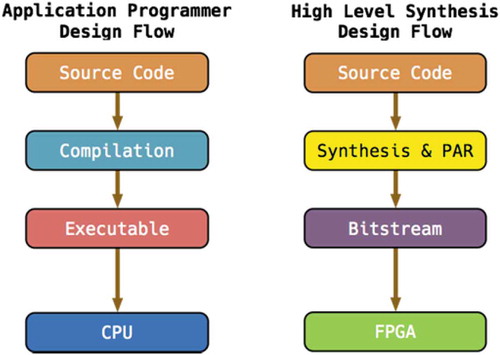
Figure 1 presents a design flow comparison between the application programmer aiming at CPU and the hardware designer targeting at FPGA (Ma et al. 2016). Application programmers normally use high-level programming languages to write source code, such as C, C++, Java, etc. Hardware description language (HDL) is the typical option for hardware designers, such as VHDL or Verilog. Nowadays, high-level synthesis (HLS) language becomes the other choice of FPGA designers (Xilinx, 2017), such as HLS C++ or OpenCL. The source can be compiled to executables targeting at specific instruction set architectures, such as X86, MIPS or ARM RISC. The source code for FPGA will be synthesized to a description of connectivity of electronic circuit, called netlist. Based on the netlist, the tools will place and route (PAR) onto the FPGA and generate the Bitstream.

Figure 1. The difference of design flow between CPU and FPGA.

In the remaining sections of this article, we first review the algorithm of MLC to be implemented in this pilot study. We will then introduce how FPGA cloud is used to implement MLC. The result of this pilot study will be summarized followed by a brief conclusion. The solutions explored in this research can be extended to other types of image-processing solutions to handle big image data.

2. Overview of MLC

MLC is a supervised image classification method based on Bayes theorem. The algorithm and implementation of MLC on different platforms were discussed in detail in a prior work (Shi & Xue, 2017). In summary, MLC measures the probability that a pixel with feature vector $\mathbf{x}$ belongs to a class and assigns the pixel to the most possible class. The following equation (Richards & Jia, 1999) calculates the probability $\mathrm{p}\left({\omega }_{\mathrm{i}}|\mathbf{x}\right)$ that pixel x belongs to class ${\omega }_{\mathrm{i}}$.

$\mathrm{p}\left({\omega }_{\mathrm{i}}|\mathbf{x}\right)=\mathrm{p}\left(\mathbf{x}|{\omega }_{\mathrm{i}}\right)\ast \mathrm{p}\left({\omega }_{\mathrm{i}}\right)/\mathrm{p}\left(\mathbf{x}\right)$

where x represents a pixel, if the image contains multiple bands, then x would be a vector. $\mathrm{p}\left({\omega }_{\mathrm{i}}\right)$ is the probability that class ${\omega }_{\mathrm{i}}$ occurs in the image. It is estimated from the training data, be arbitrarily assigned, or assumed to be equal across all classes. It is also possible to specify a probability threshold below which the pixel would not be assigned to any classes. $\mathrm{p}\left(\mathbf{x}|{\omega }_{\mathrm{i}}\right)$, the probability of observing x in class ${\omega }_{\mathrm{i}}$, can be derived from the training data. Thus,

$\mathbf{x}\in {\omega }_{\mathrm{i}}\mathrm{i}\mathrm{f}\mathrm{p}\left(\mathbf{x}|{\omega }_{\mathrm{i}}\right)\ast \mathrm{p}\left({\omega }_{\mathrm{i}}\right)>\mathrm{p}\left(\mathbf{x}|{\omega }_{\mathrm{j}}\right)\ast \mathrm{p}\left({\omega }_{\mathrm{j}}\right),\mathrm{f}\mathrm{o}\mathrm{r}\mathrm{a}\mathrm{l}\mathrm{l}\mathrm{j}\ne \mathrm{i}$

MLC assumes that the distribution of pixel digital values obeys multivariate normal distribution, that is, $\mathrm{p}\left(\mathbf{x}|{\omega }_{\mathrm{i}}\right)\text{~}N\left({\mu }_i,{\mathrm{\Sigma }}_{\mathrm{i}}\right)$, which leads to maximum likelihood estimation of $\mathrm{p}\left({\omega }_{\mathrm{i}}|\mathbf{x}\right)$:

$\text{{rm{p}}left({{{rm{omega }}\_{rm{i}}}{rm{|x}}} right) = { }2{pi ^{ - N/2}}{left| {{{rm{C}}\_{rm{i}}}} right|^{ - 1/2}}{e^{{{ - 1} over 2}{{left({{bf{x}} - {{bf{m}\_i}} right)}^t}{{rm{C}}\_{rm{i}}}^{ - 1}left({{bf{x}} - {{bf{m}\_i}} right)}}}$

Taking log on both sides, the above equation is simplified as,

${\mathrm{g}}_{\mathrm{i}}\left(\mathbf{x}\right)=ln\mathrm{p}\left({\omega }_{\mathrm{i}}\right)-\frac{1}{2}ln\left|{\mathrm{C}}_{\mathrm{i}}\right|-\frac{1}{2}{\left(\mathbf{x}-{\mathbf{m}}_{\mathrm{i}}\right)}^{\mathrm{t}}{\mathrm{C}}_{\mathrm{i}}^{-1}\left(\mathbf{x}-{\mathbf{m}}_{\mathrm{i}}\right)\left(\mathrm{E}\mathrm{q}\mathrm{u}\mathrm{a}\mathrm{t}\mathrm{i}\mathrm{o}\mathrm{n}1\right)$

Equation 1 is referred to as the determinant function as it determines the class label of pixel $\mathbf{x}$. ${\mathrm{C}}_{\mathrm{i}}$ and ${\mathbf{m}}_{\mathrm{i}}$ are sample estimates of covariance and mean in class ${\omega }_{\mathrm{i}}$. ${\mathrm{g}}_{\mathrm{i}}\left(\mathbf{x}\right)$ is the likelihood that $\mathbf{x}$ belongs to class ${\omega }_{\mathrm{i}}$. Although MLC is a linear complexity algorithm, the time cost for processing a large remote-sensing image could be prohibitive. For example, the sample data used in this study are a series of three-band aerial photos that have a spatial resolution of 0.5 m. Each tile of the image has a total of 80,000 × 80,000 × 3 = 19,200,000,000 pixels.

The following pseudocode (Shi & Xue, 2017) illustrates the implementation of MLC by serial C program. Within this code, M is the class mean values derived from the training data; C is the class covariance derived from the training data; G is the input remote-sensing image; D refers to training data; N is the number of pixels in G; L is a vector of class labels; P is a vector of class priori probabilities; O is the output classification map.

1: M = ComputeClassMean(G,D)

3: for i in 0 to N-1

4: dMax = -Inf//dMax is a variable and initialized to a minimum value2: C = ComputeClassCovariance(G,D)

5:  y = −1

6:  for j in 0 to L.size – 1

7: d = Determinant(P[j], M[j], C[j], G[i])//based on Equation 1

8: if (d > dMax)

9:     d = dMax

10:     y = j

11:  O[i] = L[y]

This work computes class covariance and class mean, respectively, and iteratively computes the class label for every pixel in the input image. Within the iteration, it computes the determinant value for each class and determines the class label for a pixel. ESRI’s ArcMap software was used to define the training data, generate sample covariance and mean values, validate the quality of both serial C program and parallelized solutions for MLC and serve as the base for performance comparison. Since the time used on processing training data is not significant, we only implement MLC for the classification task, which is time consuming over big imagery data.

3. Workflow of MLC implementation on FPGA

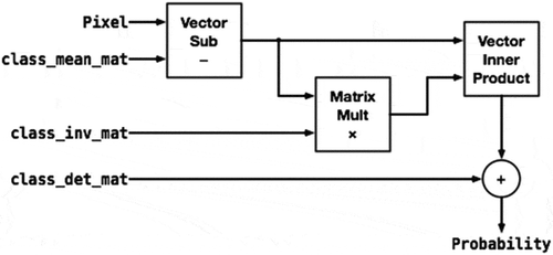
The MLC implementation on FPGA support pipelined favor and no limitation to the size of input data. We decompose the data into 1000 by 1000 pixels, and each segment is sent to the FPGA sequentially. The workflow of MLC implementation in FPGA can be abstracted as the flowchart displayed in Figure 2. In the figure, for each class, “class_mean_mat” is a vector of class means; “class_inv_mat” is the inverse of class covariance matrixes; “class_det_mat” is the determinant of class covariance matrixes; “Pixel” represents the pixel in the image as the input value. The first step of MLC is doing the vector subtraction (Vector Sub) between pixel and the vector of class means. Then, the result vector from the first step will do matrix multiply (Matrix Mult) with inverse of class covariance matrixes. The third step is doing the vector inner product on the results of previous two steps. At last, the priori probability can be calculated as the sum between the result of the third step and the determinant of class covariance matrixes.

Figure 2. Flowchart for MLC implementation in a single FPGA.

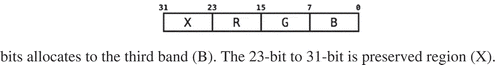
To process the three-band image, each band saves as an 8-bit data. The memory controller provided by the FPGA’s vendors normally support 4 bytes aliment by default. The minimum width of the data for each read or write operation in the memory is four bytes. Thus, for the memory aliment friendly in the FPGA, we use a 32-bit unsigned integer number to represent each pixel as displayed in Figure 3. The first band (R) locates at 16-bit to 23-bit; the second band (G) locates at 8-bit to 15-bit; the lower 8 bits allocates to the third band (B). The 23-bit to 31-bit is preserved region (X).

Figure 3. The format for each 24-bit pixel data in a 32-bit unsigned integer number.

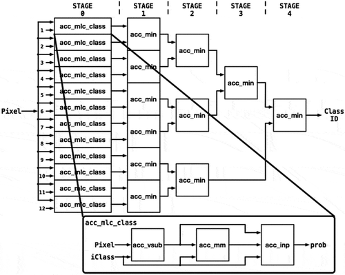
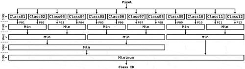
Since each function of MLC is independent, it can be pipelined to take the benefit of parallelism in FPGA. Pipeline is a typical design approach to process sequential data. The MLC implementation can be broken down to five stages (steps). Each pixel can be passed into each stage of pipeline and be processed. Based on the top-down design approach, we defined the following two functions: “acc_mlc_class” and “acc_min”. In Figure 4, function “acc_mlc_class” implements the MLC data flow. Function “acc_min” finds the minimum value. There are five states in the pipeline. In Stage 0, 12 instances of function “acc_mlc_class” will receive the input pixel simultaneously. Multiple functions of “acc_min” are instantiated in Stage 1–4 to implement a parallel reduction tree to find the minimum value.

Figure 4. Five-stage pipeline of MLC implementation.

The following C code demonstrates how to use each function in the flowchart to compute the determinant values.

1: unsigned int Get_Class(unsigned int pixel_val)

2: {

3: unsigned int iClass = 0;

4: double pixel[MAX_BAND];

5: double diffVec[MAX_BAND];

6: double diffInv[MAX_BAND];

7: double prob;

8: double PROBS[MAX_CLASS];

9:

10: pixel[0] = (pixel_val & 0x00FF0000) ≫ 16;

11: pixel[1] = (pixel_val & 0x0000FF00) ≫ 8;

12: pixel[2] = (pixel_val & 0x000000FF);

13:

14: double CUR_PROB = DBL_MAX;

15: int CUR_INDEX = 0;

16: for (iClass = 0; iClass <MAX_CLASS; iClass++) {

17: acc_vsub(pixel, diffVec, iClass);

18:  acc_mm(diffVec, diffInv, iClass);

19:  acc_inp(diffVec, diffInv, &prob, iClass);

20: PROBS[iClass] = prob;

21: if (prob ≤ CUR_PROB) {

22: CUR_PROB = prob;

23: CUR_INDEX = iClass;

24: }

25: }

26: return clsID[CUR_INDEX];

27: }

Function Get_Class takes pixel values as the input and generates the output as a class label. Lines 10–12, we used bit SHIFT and logic AND operations to extract each band’s value in each pixel. The loop block between lines 16 and 25 calculates the priori probabilities for each class. The “iClass” is the iteration variable to traverse the whole class set. The number of class is pressed by “MAX_CLASS”. Line 17, function “acc_vsub” is vector subtraction. The function “acc_mm” is matrix multiply in line 18. The vector inner product is presented by function “acc_inp” in line 19. The branch block from lines 21 to 24 derives the largest determinant values for each class. Line 26 will return the corresponding class presented in “clsID” array.

4. Implementation of MLC through high-level synthesis

Normally, the HDL is the tool to design the circuit in the FPGA. To improve the productivity of design in the FPGA, research tried to use high-level language to low the barrier of the FPGA design. HLS used C/C++ to increase the productivity for FPGA design.

The following HLS code builds the function of vector subtraction. It takes pixel and the number of class as the inputs. Based on the pixel and class number, “acc_vsub” will operate the vector subtraction on the pixel and class means. Line 5 uses “#pragma” to indicate the HLS to generate the pipelined hardware circuit for the loop block from lines 4 to 7. “class_mean_mat” is the class mean matrix, which is a number of classes by number of bands matrix. Each row of the matrix represents the means of each class and the column in each row shows the means for each bands.

1: void acc_vsub(double *pixel, double *diffVec, int iClass)

2: {

3: int i;

4: for (i = 0; i < MAX_BAND; i++) {

5: #pragma HLS PIPELINE

6: diffVec[i] = pixel[i] – class_mean_mat[iClass][i];

7:  }

8: }

The matrix multiply can be done by HLS as displayed in the following function “acc_mm.” The results from vector subtraction will be the input for “acc_mm” function, named “diffVec”. “diffInv” is the output of the function. “class_inv_mat” is the inverse of class covariance matrixes and “iClass” is used to iterate each class.

1: void acc_mm(double *diffVec, double *diffInv, int iClass)

2:{

3: int j, k;

4: int Col = MAX_BAND;

5: for (j = 0; j < Col; j++) {

6: #pragma HLS PIPELINE

7: double sum = 0.0;

8: for (k = 0; k < Col; k++) {

9:  #pragma HLS PIPELINE

10:  sum + = diffVec[k] * class_inv_mat[iClass][k][j];

11:  }

12:  diffInv[j] = sum;

13: }

14: }

The last step is the vector inner product and the HLS code of the function is presented below. The outputs of function “acc_vsub” and “acc_mm” are two vectors and will be the inputs for “acc_inp” function. The output “prob” is the priori probabilities. Line 9 calculates the results by adding the value of vector inner product and the value in the determinant of class covariance matrixes.

1: void acc_inp(double *diffVec, double *diffInv,

2:   double *prob, int iClass)

3: {

4: double sum = 0;

5: for (int i = 0; i < MAX_BAND; i++) {

6: #pragma HLS PIPELINE

7: sum = sum + diffVec[i] * diffInv[i];

8:  }

9:  *prob = sum + class_det_mat[iClass];

10: }

The top function is called “acc_mlc_class” and is used for calculating the priori probabilities for one specific class by the variable “arg”. “ap_uint<32>” declares a variable with 32 bits. Each pixel in the image is the input through the variable “sI1_V.” “mO1_V” is the output and represents the priori probability for each pixel of one class. Lines 4–7 declare the interface of inputs and outputs. “ap_ctrl_none” shows that the accelerator generated by HLS does not content the control logic. “axis” is the type steaming interface in HLS. PIPELINE passes the requirement to the HLS compiler to generate the pipelined hardware circuit. Line 16 reads one pixel from the input and values of each bands will extract in lines 17–19. The method of “input_pixel.range(x, y)” will extract the bits from x to y. Lines 21–23 follows the MLC data flow and calculates priori probabilities. The output will be assigned in line 25.

1: void acc_mlc_class(unsigned int *sI1_V, double *mO1_V,

2:      ap_uint<32> arg)

3: {

4:  #pragma HLS INTERFACE ap_ctrl_none port = return

5:  #pragma HLS INTERFACE axis depth = 16 port = sI1_V

6:  #pragma HLS INTERFACE axis depth = 16 port = mO1_V

7:  #pragma HLS PIPELINE

8:

9:  unsigned int iClass = arg;

10: ap_uint<32> input_pixel;

11: double pixel[MAX_BAND];

12: double diffVec[MAX_BAND];

13: double diffInv[MAX_BAND];

14: double prob;

15:

16:  input_pixel = *sI1_V;

17:  pixel[0] = input_pixel.range(23,16);

18:  pixel[1] = input_pixel.range(15, 8);

19:  pixel[2] = input_pixel.range(7, 0);

20:

21:  acc_vsub(pixel, diffVec, iClass);

22:  acc_mm(diffVec, diffInv, iClass);

23:  acc_inp(diffVec, diffInv, &prob, iClass);

24:

25:  *mO1_V = prob;

26: }

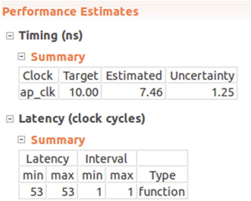
The compilation results from HLS tools are shown in Figure 5. According to the estimated performance, we get that the latency (for how long a pixel can be processed by the FPGA) for the “acc_mlc_class” function is 53 clock cycles. Clock cycle is used to calculate the execution time. For example, if a circuit is running under 100MHz, one clock cycle is 1/100MHz which is 10 ns. Thus, we can estimate how long it takes to process a pixel. The interval latency is 1 clock cycles, which means this function is pipelined. It takes 53 clock cycles to process one pixel. After the first pixel, the function can produce one output in every clock cycle.

Figure 5. Latency of “acc_mlc_class” function.

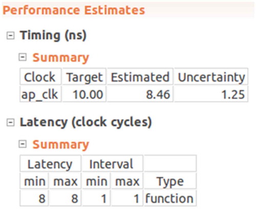
The “acc_min” function is used to find the minimum number between two inputs and passes the smaller input as the output. Since the function only has two inputs, we can cascade several functions together and to construct a new function with more inputs. The latency for function “acc_min” is two cycles. We used 11 “acc_min” functions to build a reduction tree with 4 depths. The total latency is 8 clock cycles shown in Figure 6.

Figure 6. Latency of “acc_min” reduction tree with 4 depths.

1: void acc_min(double *sI1_V, double *sI2_V, double *mO1_V)

2: {

3:  #pragma HLS INTERFACE ap_ctrl_none port = return

4:  #pragma HLS INTERFACE axis depth = 16 port = sI1_V

5:  #pragma HLS INTERFACE axis depth = 16 port = sI2_V

6:  #pragma HLS INTERFACE axis depth = 16 port = mO1_V

7:

8:  double in1 = *sI1_V;

9:  double in2 = *sI2_V;

10: *mO1_V = (in1 ≤ in2) ? in1: in2;

11: }

As displayed in Figure 7, we instantiated 12 functions named “acc_mlc_class” to take the advantage of the parallelism. Each function is used to calculate the prior probabilities of each class at the same time. Stage 0 in the figure presents the 12 functions for each class. The input pixel is transferring to each function at the same time. Two outputs from “acc_mlc_class” functions pass to a minimum function to find the smaller value from Stage 1–4. After the Stage 4, we can get the final class ID. The structure of Stage 1–4 is called reduction tree and it is a typical structure to calculate the minimum number in parallel.

Figure 7. The design flow for MLC implementation in FPGA.

The MLC design needs five stages (steps) as described in Figure 8. Based on the performance reports from HLS tools, the latency of five stages is totally 61 clock cycles. Since our implementation is based on the pipelined flavor, it takes 61 clock cycles to achieve the first results. After that, we can get new result in every clock cycle. The processing sequence of first four inputs is presented in the Table 1. At time T₀, PIXEL₁ goes in Stage 0. Later, at time t₁, Stage 0 finished and the result goes into Stage 1. At the same time, PIXEL₂ goes into Stage 0. Finally, when PIXEL₁ finished in Stage 4, PIXEL₅ is in Stage 0. After T₄, we can achieve a result at time T_x.

Figure 8. Demonstration of pixel in the pipeline of the design.

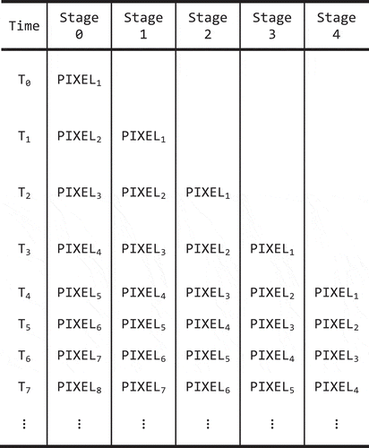
Table 1. Results of comparison between FPGA, CPU and GPU.

Implementation over 18 GB data	Hardware		Time (s)	Speedup
AHPCC CPU cluster	Intel Xeon E5-2670 2.6 GHz	100 processors	184.1
		160 processors	121.7	1.51
		250 processors	86.4	2.13
		320 processors	70.6	2.60
		400 processors	62.8	2.93
GPU	NVIDIA Tesla K40C		19.1	9.64
Micron FPGA cluster	Micron AC-510	1 FPGA	66.6	2.76
		2 FPGAs	33.4	5.51
		4 FPGAs	16.7	11.02
		8 FPGAs	8.5	21.66
		16 FPGAs	4.7	39.17
		32 FPGAs	3.0	61.37

5. Test in micron AC-510 FPGA cluster

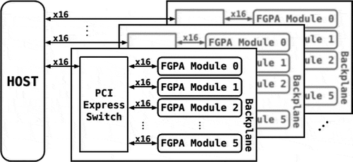
All experiments reported in this article were performed on a reconfigurable FPGA cluster developed by Micron. Figure 9 shows a simplified block diagram of Micron’s reconfigurable cluster. The host system is a dual Intel Xeon-2650 processor with 128GBs of DDR4 memory. The system runs Ubuntu 14.04 with Linux kernel 3.12.0. On the backplane, a central PCI Express switch is used to connect the FPGA boards. Each backplane is an independent PCI Express device connected to the host. The system is contained in a 4U server with six backplanes. Each backplane connects six Xilinx Ultrascale Kintex FPGAs (AC-510). All reported results are actual run time results.

Figure 9. Block diagram of Micron’s FPGA cluster architecture (Ma et al. 2016).

The C code on the PC host is presented below. Lines 2–7 are to initialize the FPGAs. The maximum number of FPGA modules is defined by MAX_MODULE variable. There are 32 FPGAs in Micron’s FPGA cluster. The streams defined in Lines block 8–13 are the interface to transfer the data from the PC to the FPGA modules. There are two streams for each FPGA module. One uses as the write stream and the other uses as the read stream. One POXIS thread is used for each stream, which defined in lines block 14–33. In lines 34–47, several threads (sub-programs) are lunched according to the multiplication of variable of nu_module and nu_stream. The nu_module presents the number of modules and nu_stream indicate the number of streams. The in_buff is the input data in line 22 and the out_buff is the output data in line 30.

1: …

2: PicoDrv *pico[MAX_MODULE];

3: PICO_CONFIG cfg = PICO_CONFIG();

4: cfg.model = 0x510;

5: for (int i = 0; i < nu_module; i++) {

6: FindPico(&cfg, &pico[i]));

7: }

8: unsigned int stream[nu_module][nu_stream];

9: for (int j = 0; j < nu_module; j++) {

10:for (int i = 0; i < nu_stream; i++) {

11: stream[j][i] = pico[j]->CreateStream(i + 1);

12:  }

13: }

14: pthread_t thread[nu_module][nu_stream][2];

15: task_pk_t task_pkg[nu_module][nu_stream][2];

16: for (int j = 0; j < nu_module; j++) {

17: for (int i = 0; i < nu_stream; i++) {

18:  //Package for write

19: task_pkg[j][i][0].Pico = pico[j];

20: task_pkg[j][i][0].Type = WS;

21: task_pkg[j][i][0].Stream = stream[j][i];

22: task_pkg[j][i][0].In_Data = &in_buff[nu_ditem/nu_module * j

+ nu_ditem/nu_module/nu_stream * i];

23: task_pkg[j][i][0].Out_Data = NULL;

24: task_pkg[j][i][0].Size = nu_ditem/nu_module/nu_stream;

25:  //Package for read

26: task_pkg[j][i][1].Pico = pico[j];

27: task_pkg[j][i][1].Type = RS;

28: task_pkg[j][i][1].Stream = stream[j][i];

29: task_pkg[j][i][1].In_Data = NULL;

30:  task_pkg[j][i][1].Out_Data = &out_buff[nu_ditem/nu_module * j + nu_ditem/nu_module/nu_stream * i];

31: task_pkg[j][i][1].Size = nu_ditem/nu_module/nu_stream;

32:  }

33: }

34://Created Threads

35: for (int j = 0; j < nu_module; j++) {

36: for (int i = 0; i < nu_stream; i++) {

37: pthread_create(&thread[j][i][1], NULL, Stream_Threads_Call, (void *)&task_pkg[j][i][1]);

38: pthread_create(&thread[j][i][0], NULL, Stream_Threads_Call, (void *)&task_pkg[j][i][0]);

39:}

40:}

41://Joined Threads

42: for (int j = 0; j < nu_module; j++) {

43: for (int i = 0; i < nu_stream; i++) {

44: pthread_join(thread[j][i][0], NULL);

45: pthread_join(thread[j][i][1], NULL);

46:  }

47: }

48: …

6. Results

Table 1 lists the execution time of MLC on CPU cluster, NVIDIA K40 GPU and FPGAs cluster. We only counted image classification time. Overhead, synchronization and data transfer outside image reading and writing were excluded in the classification time. Table 1 indicates that significant speedups were achieved by parallel implementations. We take the MPI approach with 100 processors as the baseline; the maximum speedup of about 2.93 was achieved when using 400 processors on Arkansas High Performance Computing Center (AHPCC) cluster. The K40 GPU achieved a speedup of approximately 9.64 in comparison to the MPI approach on 100 CPU processors. FPGA seems to be the best solution for parallelized MLC as the maximum speedup of about 61.37 was achieved when 32 FPGAs were used in comparison to 100 CPU processors.

Generally, the implementation of MLC by MPI, GPU and FPGA partitions the input image into segments, while different solutions are employed to read, classify and write data. In the MPI implementation, data segments are loaded into the memory of each processor independently and are classified simultaneously by all processors. However, pixels in one data segment are processed in sequential order by one processor. In the implementation of MLC on GPU and FPGAs, data segments are accessed in sequential order, while one segment is classified in parallel.

As shown in Table 1, the execution time of the MPI implementation decreased when more processors were used. There is no significant speedup between 400 and 320 processors given the current implementation. GPU displays its superior in image classification even in comparison to the work done by 400 CPU processors.

The performance of FPGA cluster reveals linear scalability between 1 and 16 FPGAs. Due to the I/O bandwidth limitation in the cluster system, the performance stops linear increase when using 32 FPGAs. But we can achieve a total of 61.37 speedup in comparison to the work done by 100 CPU processors.

7. Conclusions

MLC is data intensive and highly parallelizable. Such an algorithm is highly suitable to FPGA, which employs multiple pipelined processing element and wide bandwidths on the Micron FPGA cluster. In comparison to CPU clusters, FPGA is more accessible and less energy consuming. One potential bottleneck for MLC calculation on a FPGA cluster is the limit of bandwidth of PCIe. Even if there is streamed pipeline structure in the FPGA, the image data have to break into segments and be processed separately through PCIe bus. Repeatedly transferring data from PC to FPGA causes additional time and lowers down the speedups. Moreover, the number of threads that can simultaneously run on a PC is limited.

Data availability statement

The imagery data used in this study are a series of aerial photos captured in 2007 covering the metropolitan area of Atlanta and may be available at Georgia GIS Data Clearinghouse. Readers may apply any other remotely sensed imagery data to test the proposed solution.

Disclosure statement

No potential conflict of interest was reported by the authors.

Additional information

Funding

This research was partially supported by the National Science Foundation through the award SMA-1416509.

References

- Boschetti, M., Boschetti, L., Oliveri, S., Casati, L., & Canova, I. (2007). Tree species mapping with airborne hyper-spectral MIVIS data: The Ticino Park study case. International Journal of Remote Sensing, 28(6), 1251–1261.
- Buddenbaum, H., Schlerf, M., & Hill, J. (2005). Classification of coniferous tree species and age classes using hyperspectral data and geostatistical methods. International Journal of Remote Sensing, 26(24), 5453–5465.
- Clark, M. L., Roberts, D. A., & Clark, D. B. (2005). Hyperspectral discrimination of tropical rain forest tree species at leaf to crown scales. Remote Sensing of Environment, 96(3), 375–398.
- George, N., Lee, H., Novo, D., Rompf, T., Brown, K., Sujeeth, A., … Ienne, P. 2014. Hardware system synthesis from domain-specific languages. In Proceedings of 2014 24th International Conference on Field Programmable Logic and Applications (FPL) (pp. 1–8).
- Greenberg, J., Dobrowski, S., & Vanderbilt, V. (2009). Limitations on maximum tree density using HSR remote sensing and environmental gradient analysis. Remote Sensing of Environment, 113, 94–101.
- Guan, Q., Shi, X., Huang, M., & Lai, C. (2016). A hybrid parallel cellular automata model for urban growth simulation over GPU/CPU heterogeneous architectures. International Journal of Geographical Information Science, 30(3), 494–514.
- Ma, S., Aklah, Z., & Andrews, D. 2016. Just in time assembly of accelerators. In Proceedings of the 2016 ACM/SIGDA International Symposium on Field-Programmable Gate Arrays (pp. 173–178). New York, NY USA: ACM 2016.
- Ma, S., Andrews, D., Gao, S., & Cummins, J. 2016. Breeze computing: A just in time (JIT) approach for virtualizing FPGAs in the cloud. In Proceedings of the 2016 International Conference on ReConFigurable Computing and FPGAs (ReConFig) (pp. 1–6). Cancun, Mexico. doi: 10.1109/ReConFig.2016.7857159
- Martin, M., Newman, S., Aber, J., & Congalton, R. (1998). Determining forest species composition using high spectral resolution remote sensing data. Remote Sensing of Environment, 65(3), 249–254.
- Richards, J. A., & Jia, X. (1999). Remote sensing digital image analysis (Vol. 3). Berlin Heidelberg: Springer. doi:10.1007/978-3-662-03978-6
- Shi, X., Huang, M., You, H., Lai, C., & Chen, Z. (2014a). Unsupervised image classification over supercomputers Kraken, Keeneland and Beacon. GIScience & Remote Sensing, 51(3), 321–338.
- Shi, X., Lai, C., Huang, M., & You, H. (2014b). Geocomputation over the emerging heterogeneous computing infrastructure. Transactions in GIS, 18(S1), 3–24.
- Shi, X., & Xue, B. (2017). Parallelizing maximum likelihood classification on computer cluster and graphics processing unit for supervised image classification. International Journal of Digital Earth, 10(7), 737–748.
- Sridharan, H., & Qiu, F. (2013). Developing an object-based HSR image classifier with a case study using worldview-2 data. Photogrammetric Engineering & Remote Sensing, 79(11), 1027–1036.
- Thenkabail, P. S., Enclona, E. A., Ashton, M. S., Legg, C., & De Dieu, M. J. (2004). Hyperion, IKONOS, ALI, and ETM+ sensors in the study of African rainforests. Remote Sensing of Environment, 90(1), 23–43.
- Xiao, Q., Ustin, S., & McPherson, E. (2004). Using AVIRIS data and multiple-masking techniques to map urban forest tree species. International Journal of Remote Sensing, 25(24), 5637–5654.
- Xilinx. 2017. UG902 Vivado Design Suite User Guide: High-Level Synthesis. Retrieved 18 April 2018 from https://www.xilinx.com/support/documentation/sw_manuals/xilinx2017_1/ug902-vivado-high-level-synthesis.pdf