A survey of analytical methods for inclusion in a new energy-water nexus knowledge discovery framework

ABSTRACT

The energy-water nexus, or the dependence of energy on water and water on energy, continues to receive attention as impacts on both energy and water supply and demand from growing populations and climate-related stresses are evaluated for future infrastructure planning. Changes in water and energy demand are related to changes in regional temperature, and precipitation extremes can affect water resources available for energy generation for those regional populations. Additionally, the vulnerabilities to the energy and water nexus are beyond the physical infrastructures themselves and extend into supporting and interdependent infrastructures. Evaluation of these vulnerabilities relies on the integration of the disparate and distributed data associated with each of the infrastructures, environments and populations served, and robust analytical methodologies of the data. A capability for the deployment of these methods on relevant data from multiple components on a single platform can provide actionable information for interested communities, not only for individual energy and water systems, but also for the system of systems that they comprise. Here, we survey the highest priority data needs and analytical methods for inclusion on such a platform.

KEYWORDS:

• Energy-water nexus
• data
• analytics
• web portal

1. Introduction

The energy-water nexus, or the dependence of energy on water and water on energy, continues to receive attention as impacts on both energy and water supply and demand from growing populations and climate-related stresses are evaluated for future infrastructure planning (Scanlon et al., 2017). These impacts have been studied extensively using integrated assessment, infrastructure risk simulation, integrated analysis, and risk analysis. Among the findings of these studies is the realization that the vulnerabilities of energy-water systems and impacts to them are deeper and more intricate than those that directly affect their physical infrastructures. Impacts of extreme weather and climate events to these systems extend to economic, social and environmental services provided by them. Consequences can include disrupted supply chains, suspended economic activity, and threats to social well-being (Wilbanks & Fernandez, 2014). Moreover, there are feedbacks between water and energy flows that are influenced by population shifts, regional economic development, urbanization and infrastructure dynamics, land use and landcover change, policy and institutional changes and stakeholder and consumer preferences. (Figure 1).

Figure 1. Modeling at the energy-water nexus (adapted from Vallario (2017)).

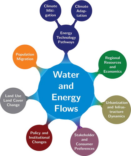
Different component functions contribute to the Energy-Water Nexus: energy production and conversion, energy use, energy disposition, water withdrawal and consumption, water treatment, and water disposition. These components interact in complex ways as physiographic, socioeconomic and infrastructure constraints to this system change under temperature rise, altered regional precipitation patterns and shifts in populations and demand centers (Allen, Fernandez, Fu, & Olama, 2016; McGranahan, Balk, & Anderson, 2007; Warner, Ehrhart, Sherbinin, Adamo, & Chai-Onn, 2009). Thus, concerns over equity, efficiency and economics of energy and water use, technological innovation, and supply versus demand dominate discussions among a variety of interested communities (National Research Council, 2010; Gleick, 1994; McManamay et al., 2017; Tidwell, Kobos, Malczynski, Hart, & Klise, 2009). Energy and water professionals such as transmission planners, utility planners, project developers, and university researchers have a need to understand the interactions among water and energy as they plan for future development that emphasizes adaptive capacity and minimizes vulnerability.

1.1. Components of the energy-water nexus and their interaction within a knowledge discovery framework

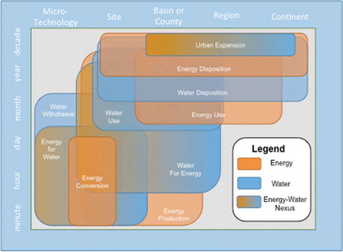
What has been missing from this type of planning and research is a capability for integrating data, models, and maps used by disparate groups for vulnerability and impact assessment, and a powerful toolset for mining large data sets (big data) pertaining to human geography, climate and other factors. We propose a new capability, served through a web-based common framework, that can provide access to appropriate data (“big” and “small”), standardized and seamless data management with quality assurance to users, along with advanced and interoperable data analytics including machine learning and pattern recognition, and advanced visualization capabilities. This co-located and accessible suite of tools could be used to pursue appropriate and cost-effective water and energy resource resilience investments at different scales using reproducible methods and maintaining data provenance. Figure 2 shows a notional summary of the temporal and spatial scales at which each of the infrastructures are typically modelled. The orange boxes represent the energy sector, while the blue boxes represent the water sector. Interaction among different components of each sector are evident at each scale. Areas of overlap depict the potential for this interaction. Within the framework, as models from each of these sectors at each scale are run, consideration for spatial and temporal boundaries of each system and how they overlap (such as locations of natural resources and how they are distributed across natural, political or infrastructure boundaries) would be managed for interpreting and validating results from coincident analysis of multiple systems. Such validation and interpretation would be built into the framework and explicitly documented.

Figure 2. Notional Summary of Spatial and Temporal Scales for Various Analyses of Energy-Water Nexus Issues. Orange boxes represent the energy sector; blue boxes represent the water sector.

The architecture needed for an Energy-Water Nexus Knowledge Discovery Framework requires accommodation of cross-cutting needs such as an ability to publish and archive data, support for analysis across heterogeneous data sets, and the enabling of effective access mechanisms across facilities. Ideally, the system should serve as a virtual laboratory and collaborative ecosystem for a variety of users. This suite of analytics should ultimately be capable of, for example, 1) optimizing freshwater/gray water use in energy production, electricity generation, and end use systems; 2) increasing the energy efficiency of water management, treatment, distribution, and end use systems; 3) promoting responsible energy operations with respect to water quality and ecosystems; 4) exploiting productive synergies among water and energy systems; 5) enhancing the reliability and resilience of energy and water systems, especially under intensifying extreme weather events; 6) optimizing costs and benefits for emerging technology; and 7) considering implications for the energy-water nexus under urban expansion. Thus, distributed mechanisms for computing, the ability to have distributed data sets and access and dissemination mechanisms are integral to the framework.

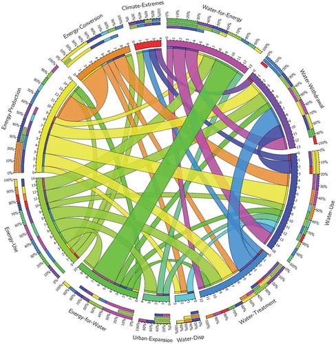
Here, we survey the literature on energy-water nexus research to discover the most common data and tools used for analysis in this area along with emerging tools to uncover new patterns. We focus on understanding relevant processes and identifying vulnerabilities in and among these systems, and we discuss the integration of these data and tools into a single platform. Figure 3 relates the various energy and water sector focus areas by the types of tools common to traditional analysis of each (as reported in the literature), and offers a visual representation of the relationship of each pair. The thickness of each connecting line represents the number of analytical tools in common between the each pair of focus areas. Each focus area is indicated by a different color. The outer ring labels give each focus area. Percentages on the outermost thin rings correspond to the percentage of tools each focus area shares with each other area. The other two thin rings partition the percentages into connections shown as inreaching and those shown as outreaching. The number of tools each area shares with at least one other area is shown in the thick rings spanning each focus area. Tools shown to be in most common use across focus areas, then, should be prioritized for inclusion in a knowledge discovery framework.

Figure 3. Circos diagram showing categories related by analytical method. Thickness of connecting lines is based on the number of common analytical methods used by each category pair.

2. Energy-water interdependence

To provide a comprehensive tool that allows an integrated view of energy and water resource management, i.e. one that couples the complex physics governing resource supply with the diverse social and cultural values defining resource demand, we must consider in detail the interdependencies between the two infrastructure sectors.

Analytics used to approach these issues have traditionally comprised primarily empirical and statistical methods. Empirical methods rely on direct and indirect observation or measurements, and include both quantitative and qualitative approaches. Statistical models often provide a first quantitative glimpse at relationships among a set of selected parameters under study (Tso & Yau, 2007). These methods tend to fall into four broad categories: parametric and non-parametric probability distribution (PDF) fitting, time series analysis, linear and non-linear regression, and machine learning techniques. A PDF represents the probability that a given parameter takes a specific value. Time series are used primarily to obtain an understanding of the underlying forces and structure that produce a specific set of observed data, and to fit a model for forecasting future similar data (NIST, 2017). Regression analyses summarize relationships between two or more variables (predictand and predictor(s)) using weights to represent greater influence of one predictor over another. Machine learning relies on pattern recognition and includes some regression methods, but extends further to include iterative learning algorithms allowing independent computational adaptation to data (SAS, 2017). Metrics for evaluating these methods are numerous. Some examples include Root Mean Square Error (RMSE) and Receiver Operating Characteristic (ROC) curves. RMSE is one of the most widely used metrics to measure discrepancy between data sets. For energy-water nexus problems, it usually measures the error between model predicted values and observed values. ROC curves are used to diagnose the predictive fitness of a model. ROC curves plot the true positive rate of prediction as a function of the false positive rate and identify the level at which the function is maximized or at which the highest true positive to total diagnoses (sensitivity) is met (Murphy, 1996; Peres & Cancelliere, 2014). Such evaluations, and potentially others, would be a necessary part of an integrated framework for any type of data analysis.

We discuss in Section 2 ways in which various data and methods have been applied to various aspects of the energy-water nexus, and which should be prioritized for inclusion in a common framework. We follow up with conclusions regarding the establishment of such a framework in Section 3.

2.1. Data and methods for evaluating energy supply for electricity generation

Characterization and prediction of energy supply and demand patterns and trends, along with identification of disposition of natural resources and siting for generation are urgent needs, as energy use and economic development are closely correlated, and access to energy is essential to quality of life in and among nations (Allouhi et al., 2015). Energy is produced using many different fuel sources: fossil (e.g. petroleum, natural gas, coal), nuclear, hydropower, wind, solar and other renewables. Which type of fuel is used in a given region has to do with natural resources available and in-place and proposed infrastructure and policy (BERC, 2017). Thus, we examine first the tools used to determine fuel available to serve electricity production needs.

Fossil fuels are limited and non-renewable resources; thus, understanding the lifetime of these resources is critical for planning. The importance of estimating the availability of these resources is reflected in the data made available by the Energy Information Administration (EIA) Annual Energy Outlook https://www.eia.gov/outlooks/aeo/, which includes estimates of initial production (IP) rates and production decline curves, which determine estimated ultimate recovery (EUR) per well. Given the EUR and an established length of time, a Gaussian or other suitable PDF may be constructed to represent the amount of a resource available for any particular year. M. King Hubbert proposed this method during the 1950s (Hubbert, 1949) to identify a time period during which the United States could expect peak output of petroleum from its domestic sources (“Peak Oil”) (Vanek, Albright, & Angenent, 2008). Hubbert later applied this technique to projected availability of natural gas and nuclear sources (Hubbert &  Shell  Development  Co. 1956). Because some electricity providers have replaced retired coal power plants with natural gas combined cycle, additional data-driven estimates of natural gas EUR have become important. Based on independent data obtained from the Barnett Shale Play (Ikonnikova, Browning, Horvath, & Tinker, 2014), Original free Gas In Place, EUR and 30-year cumulative production (Q) have been estimated using equations based on previously determined geologic parameters. Thus, including access to public data through appropriate authentication procedures, along with a provision for uploading user obtained data sets is important for analysis of this type.

Wind speed frequency for wind power estimates are most often performed using a PDF fit (Weibull or Rayleigh) of wind time series (e.g. Akpinar & Akpinar, 2005; Ayodele, Jimoh, Munda, & Agee, 2012; Billinton, Chen, & Ghajar, 1996; Celik, 2004) obtained from meteorological station measurements https://www.ncdc.noaa.gov/data-access/land-based-station-data/land-based-datasets/global-historical-climatology-network-ghcn. Additionally, Kalman filters (Ding, Zhang, & Wu, 2005; Tian, Liu, Hu, & Liao, 2014) and Box-Jenkins analyses, including autoregressive (AR), moving average (MA), autoregressive moving average model (ARMA) (Rajagopalan & Santoso, 2009; Torres, Garcia, De Blas, & De Francisco, 2005), and autoregressive integrated moving average model (ARIMA) (Kavasseri & Seetharaman, 2009; Lei, Shiyan, Chuanwen, Hongling, & Yan, 2009) schemes are used for making predictions. These techniques are used for building state-space models, which predict subsequent values from a current state, estimate current values of the state from past and current observations, and/or estimate past values of the state given a set of current observations. https://www.quantstart.com/articles/State-Space-Models-and-the-Kalman-Filter

Traditional statistical methods are trusted for these analyses, so inclusion of these methods in an integrated tool is reasonable. However, increasingly, machine learning is more successfully applied to such assessments. For example, machine learning methods such as Artificial Neural Networks (ANN) Barbounis and Theocharis (2007); Hervás-Martínez et al. (2009); Kariniotakis, Stavrakakis, and Nogaret (1996); Li and Shi (2010); Welch, Ruffing, and Venayagamoorthy (2009), fuzzy systems Damousis, Alexiadis, Theocharis, and Dokopoulos (2004); Foley, Leahy, Marvuglia, and McKeogh (2012), and support vector machines (SVM) Chang (2014); Zeng and Qiao (2011) have also been applied successfully to short-term wind power forecasting. In windspeed and wind power forecasting, these techniques are used to help reduce loss of load events, to increase fuel savings and to make optimal use of available wind energy (Kariniotakis et al., 1996). Fuzzy systems are used in wind power prediction to provide future estimates of wind speed at a given site based on recent variations of wind speed at neighboring sites (Damousis et al., 2004). Support Vector Machines (SVM) applied to short-term windpower forecasting predict future windspeed from current observations. Results are then used to estimate expected power generated.¹

Hydropower is subject to water availability affected by different variables such as precipitation patterns, streamflow, hydraulic head, and volume of water storage available. Measured data for these variables is available through agencies such as the United States Geological Survey https://waterdata.usgs.gov/nwis/rt and analogues in other countries. Methods for predicting rainfall intensity contributing to streamflow include various parametric PDF fitting procedures using primarily the Gamma distribution or the Log-Pearson III distribution. Choice of function usually depends upon temporal resolution (10-minute intervals to monthly or annual averages) of the measured data (Kao & Ganguly, 2011).²

Additionally, machine learning algorithms are applied to hydropower problems, including Support Vector Machines (SVM) (Mohandes, Halawani, Rehman, & Hussain, 2004; Tay & Cao, 2002; Tripathi, Srinivas, & Nanjundiah, 2006), ANNs (French, Krajewski, & Cuykendall, 1992; Lin & Chen, 2004; Luk, Ball, & Sharma, 2000; Pan & Wang, 2004; Ramirez, de Campos Velho, & Ferreira, 2005), RANNs (Recurrent Artificial Neural Networks) (Elman, 1990; Jordan, 1986; Kechriotis, Zervas, & Manolakos, 1994; Tsoi & Back, 1994; Williams & Zipser, 1989), and combinations of these methods (Hong, 2008; Tripathi et al., 2006). Because of the non-stationarity of rainfall trends due to ongoing changes in climate, dynamic SVMs can be used to gain understanding of these changing patterns (Cao & Gu, 2002). For handling data (e.g. rainfall) for which the underlying mathematical formulae and prior knowledge of the relationship between predictors and predictand is unknown, ANNs can provide insight into patterns.³

Principal Component Analysis (PCA) is a multivariate technique used for estimating which predictor variables contribute most to a predictand. While this technique is useful across the entire Energy-Water Nexus, it has been applied particularly extensively to rainfall calculations (e.g. Basalirwa, 1995; Dyer, 1975; Munoz-Diaz & Rodrigo, 2004; Ogallo, 1989). The method extracts information from data and represents it as a set of orthogonal vectors in which the first principal component vector explains the most variability in the data and each successive principal component explains successively less variability.⁴

Solar photovoltaic (PV) systems are projected to generate up to 16% of the worlds electricity by 2050 while solar thermal electricity (STE) from concentrating solar power (CSP) plants could provide an additional 11%, together preventing the emission of more than 6 billion tonnes of carbon dioxide per year by 2050 (International Energy Agency, 2014). Thus, many data generation and analytical techniques have been applied to predictions of regional solar energy resource and power generation. For example, EIA⁵ archives and makes available past records of net generation from renewable sources including solar photovoltaic (PV). Also, the US National Renewable Energy Laboratory (NREL)⁶ has produced synthetic solar photovoltaic (PV) power plant data points for the United States that represent a given year (e.g. 2006). These data are used to perform solar integration studies for estimating hypothetical power production from new generation and compared to the EIA reports of actual past production. All of these data can and should be made available for an integrated energy-water platform for analysis. Such analysis could include the simple cloudy model, which uses measurements of total cloud amount (Augustine, Hodges, Cornwall, Michalsky, & Medina, 2005; Bedacht, Gulev, & Macke, 2007; Boilley & Wald, 2015) to evaluate global solar irradiance Badescu (1997); or past-predicts-future (PPF) models for projecting future seasonal solar energy available based on past availability (Sharma, Sharma, Irwin, & Shenoy, 2011), or an application of multiple statistical models to a problem that can reduce bias inherent in inductive learning algorithms accommodating the range of performance across domains. Ensembles of regressions thus perform better than a single regression type on a given problem (Hossain et al., 2012). For example, an ensemble-based hybrid approach to predicting short-term (6 h ahead) solar energy availability is applied by (Hossain et al., 2012) for managing smart grid energy. The hybrid predictor method comprises methods such as SVM, RBF, linear regression, simple linear regression, additive regression (AR), and a variety of other methods using the general workflow shown in Figure 4. Results give an improvement in prediction accuracy over single-method approaches to PV solar power estimates.

Figure 4. Solar power regression ensemble workflow (adapted from Hossain, Oo, and Ali (2012)).

For all of the assessments of available fuel for electricity production, it is shown that standard statistical methods are used. In some cases, these methods are improved upon by machine learning methods. Making at least the most commonly used of these methods available through the framework is a priority for the community of practice.

2.2. Data and methods for estimating electricity demand

As of 2017, the residential and commercial buildings in the United States (U.S.) collectively consumed 38% of total U.S. energy, topping the energy usage of each of the transportation and industry sectors⁷. Residential energy consumption accounts for 20% of that consumed by all sectors. The commercial building sector in the U.S. accounts for 18% of U.S. energy use and is the fastest growing demand sector, adding nearly 1.6 billion square feet of commercial buildings per year (Griffith et al., 2008; U.S. Department of Energy, 2010). Additionally, the commercial sector is much more heterogeneous than the residential sector, with building types ranging from hospitals and schools to offices and lodging (U.S. Department of Energy, 2010). The total energy bill for these buildings was nearly $369 billion in 2005, and has continued to grow at a fast pace (U.S. Department of Energy, 2010).⁸

In response to the ever-growing energy demand from U.S. buildings, researchers have developed several approaches to understand regional demand patterns and to project demand changes for the future. Among the critical parameters considered in these studies are the spatial distribution of residential and commercial consumers, projections for future changes in those distributions, and historical and projected changes in the distribution of temperatures (Auffhammer & Aroonruengsawat, 2012). Some studies have also looked at electricity use as a function of latitude (Allen et al., 2016), while others have examined impacts of the adoption of air conditioning in more northern regions in response to increases in overall average temperature (Biddle, 2008; Rapson, 2014; Sailor & Pavlova, 2003). To evaluate demand at higher spatial resolution and by energy sector, statistical models, typically based on socio-economics, economic growth, building size, and energy prices have been employed. The majority of these modeling strategies can be grouped into top-down and bottom-up approaches, and consider data such as physical characteristics of dwellings, the socio-economic background of occupants and their appliances, historical energy consumption, climatic conditions, and macroeconomic indicators (Swan & Ugursal, 2009).⁹

The first of these approaches, top-down approaches, describe the residential energy system in terms of aggregate relationships derived empirically from historical data (Rivers & Jaccard, 2005) typically based on macroeconomic indicators, climatic conditions, housing construction rates, housing demolition rates, estimates of appliance ownership and number of units in the residential sector (Swan & Ugursal, 2009). Hirst, Lin, and Cope (1977) developed an annual housing energy model for the U.S. based upon econometric variables and the growth and contraction of housing stock. This model was later improved by including housing and technology variables (Hirst, 1978). A similar model was developed for New Zealand (Saha & Stephenson, 1980) that determined annual energy consumption of for different fuel types by analyzing ownership, stock, appliance ratings and use. Labandeira, Labeaga Azcona, and Rodr´Iguez M´Endez (2005) developed a regression model for Spanish energy demand based on demographic, macroeconomic, and climate variables from a survey of 27,000 houses, and Siller, Kost, and Imboden (2007) created a model of the Swiss residential sector to analyze the impacts of renovations and new construction on energy consumption.

Bottom-up models, on the other hand, consider technologies and processes (Rivers & Jaccard, 2005), and typically depend on macroeconomic information, energy price and income variables, individual dwelling information, and other regional and national indicators. Many bottom up approaches use samples of houses and demographic information to regress the relationships between end-uses and energy-consumption using statistical techniques such as regression, conditional demand analysis (CDA), and neural networks (Swan & Ugursal, 2009). For example, a regression model (Tonn & White, 1988) was used to analyze data from 100 sub-metered homes and 200 survey questions that depended on variables such as wood use, indoor temperature, and occupants self-defined ethical behavior and socioeconomic statuses. Later, Fung, Aydinalp, and Ugursal (1999) used regression to determine the impact of energy price, demographics, weather, and equipment on residential energy consumption, and Aydinalp-Koksal and Ugursal (2008) constructed a national Canadian residential CDA model based on 8,000 records from a Canadian national residential energy consumption survey. In 2005, Yang, Rivard, and Zmeureanu (2005) predicted building energy use by constructing an adaptive neural network that adjusted itself to unexpected pattern changes in input data. More recently, in 2016, Morton, Nagle, Piburn, Stewart, and McManamay (2016, 2017) developed a hybrid dasymetric and machine learning approach for high-resolution residential electricity consumption modeling that depended on household characteristics and national electricity consumption surveys.

The methods cited in this section are primarily economic, but their basic functionality is statistical in nature and they rely to a large extent on regression techniques. This presentation reinforces the need to include capabilities for (especially multivariate) regression in a framework that analyzes cross-sectoral data.

2.3. Data and methods for estimating water supply and demand

Rivers, lakes, reservoirs, and aquifers supply water to all human and ecological systems. The largest withdrawal of these water resources is for thermoelectric power, the second is for irrigation and the third is for the public supply (Dieter et al., 2018). Water withdrawal is the abstraction of water from groundwater or surface water sources. Water required for commercial, industrial and residential purposes requires some degree of treatment prior to use. The degree of treatment depends on water quality, source and intended end use. After the water treatment process, the water is distributed to the end users: residential, commercial and industrial. Water disposition plays an important role in the water system, as a consumer’s proximity to water supply necessarily affects its ability to satisfy its demand.

Analytical tools used for water withdrawal fall into these categories: data summary (mean, median, variance, skewness), regression (simple and multiple, linear and nonlinear), trend analysis (probability over time), and machine learning. Methods used for analysis of water withdrawal in the first three of these categories are well described by the US Geological Survey in its Statistical Methods in Water Resources (Helsel & Hirsch, 2002). These basic methods are used frequently by analysts (e.g. Sanders & Webber, 2012; Spang, Moomaw, Gallagher, Kirshen, & Marks, 2014; Stillwell, King, Webber, Duncan, & Hardberger, 2011) and should be included in an energy-water analytical framework.

Machine Learning. A primary machine learning technique used for water withdrawal analysis is an extension of decision tree analysis known as random forests. Random forests start with classification trees, types of decision trees that can be grown together as a “forest” in a computational system. They are a powerful statistical classifier with many benefits for ecological and hydrological application (Breiman, 2001; Cutler et al., 2007; McManamay, 2014; McManamay et al., 2017). The method is capable of high classification accuracy, characterization of complex predictor variable interactions, flexible analytical technique selection, and appropriate missing value handling. McManamay (2014) apply this procedure to hydrological networks to quantify and generalize hydrologic responses to dam regulation, and they find that this method is capable of generalizing the directionality of hydrologic responses to dam regulation and providing parameter coefficients to inform future site-specific modeling efforts.

PCA (described in Section 2.1) is applied to processes related to the water sector by, e.g. Carle, Halpin, and Stow (2005); Evans, Guthrie, and Videbeck (2008); Lam, Wan, Cheung, and Yang (2008); McManamay et al. (2017); Ndiaye and Gabriel (2011); Parinet, Lhote, and Legube (2004). Specifically, (McManamay et al., 2017) use principal components to calculate a cumulative hydrologic alteration index (from a seasonal hydrologic alteration index) for 250 nonreference hydrological gages based on multi-dimensional measurements. Indices describe different aspects of the hydrograph, including the magnitude, timing, frequency, duration, and rate of change in flow.

Diagnostics used to verify the fitness of these models can include R-squared, F-tests, Root Mean Square Error, residual plots, leverage statistics, model covariance, and more (e.g. Helsel & Hirsch, 2002). For comparison of model quality across all combinations of predictors included in a multiple linear regression, model scoring mechanisms based on maximum entropy or maximum likelihood (e.g. Akaike Information Criterion (AIC), Bayesian Information Criterion (BIC), Information Complexity (ICOMP)) can be used for model selection. Scores produced by these methods reward parsimony and parameter stability, and penalize parameter redundancy and bad scaling (Bozdogan, 2000).

Water allocation is managed by sector: residential, agricultural, commercial, industrial, recreational and environmental; and calculations of water use are made along the same divisions (Worthington, 2010). All water sectors are important, but three of them are particularly significant, the residential, the commercial, and the industrial. The residential sector is important because it makes up the largest water-using sector in most urban centers. The commercial and industrial sectors (combined here) are important because of the strong relationship between those sectors’ water use and economic productivity (Solley, Pierce, & Perlman, 1998; Worthington, 2010), worthington2010commercial. Thus, analyzing and forecasting residential, commercial and industrial water demand is a complex and crucial task for ensuring both a reliable water supply and economic success (HousePeters and Chang, 2011; Worthington, 2010). We focus the following two subsections on water use analytics in these sectors.

Residential Water Use. Residential water demand management has become increasingly important for decision-makers worldwide. Population growth, reductions in freshwater supplies, increasing costs of infrastructure, and the impact of climate change have prompted both suppliers and policy makers to place renewed emphasis on demand management through pricing structures and other strategies to control consumption (Worthington & Hoffmann, 2006). Consequently, the literature on modeling demand-side residential water management has grown in both depth and breadth, with the majority of studies focusing on the significance of socioeconomic variables, physical housing characteristics, outdoor water use, and climate variability for predicting residential water demand (House-Peters, Pratt, & Chang, 2010). For example, Schleich et al. (Schleich & Hillenbrand, 2009) used cross-sectional data based on economic, environmental and social variables to estimate a standard aggregate water demand mode for utility districts. Tinker et al. (Tinker, Bame, Burt, & Speed, 2005) employed multivariate stepwise regression based on temperature, rainfall, evaporation, home square footage, lot square footage, and pool data to determine monthly household water consumption.(Tinker et al., 2005). Zhang et al. (Zhang & Brown, 2005) conducted a multivariate regression analysis to analyze the effects of household water amenities and facilities, household water using habits and behaviors, household water perceptions and environmental attitudes on water use. Balling and Gober (Balling, Gober, & Jones, 2008) developed a time series of monthly water use anomalies and compared them with monthly anomalies of temperature, precipitation, and the Palmer Drought Hydrological Index. At the residential building level, water demand for provinces in Korea is forecast by (Suh, Kim, & Kim, 2015)using a backpropagation neural network (BPNN). Data inputs include shape, size and structure of the local residential buildings and water supplying infrastructures. The study explores the distinctive factors of specific apartment buildings in relation to their water use and proposes an estimation methodology that can forecast the usage amounts of water for a variety of residential structures seen in Korea.

Commercial/Industrial Water Use. Because of increasing costs for development of potable water sources, commerce and industry strive for conservation through improvements in water-use efficiency (Renzetti, 2003). Unfortunately, due to limited data in the commercial water sector, very little empirical work has gone into estimating current and future commercial and industrial water demand (Worthington, 2010). Despite these challenges, there has been some progress in this area. For example, Lynn et al. (Lynn, Luppold, & Kiker, 1979) used a mail survey of commercial firms in Miami to understand the impact of prices on water use; Schneider and Whitlatch (1991) used account-specific data for 16 Ohio communities to determine short and long-run price elasticities of commercial demand; and Malla and Gopalakrishnan (1999) estimated price and output elasticity for commercial water demand in Hawaii. Furthermore,, Williams and Suh (1986) used multivariate regression to find that aggregate residential demand was a function of marginal and average prices, the size of the customer class, per capita income, total rainfall during summer, average temperature during summer, population per square middle, industrial value-added, and receipts in establishments of selected services.

2.4. Integration of energy and water data and methods for combined assessment

Multiple researchers have suggested that integrated approaches to analyzing interactions among energy, water, climate and human activity are needed (e.g. Dale, Efroymson, & Kline, 2011; Perrone, Murphy, & Hornberger, 2011). In some cases it has been shown that this lack of integration in energy and water resource assessments results in inconsistent strategies and inappropriate allocation of resources (e.g. Howells et al., 2013). In an effort to understand energy and water coupled systems, several coupled modeling efforts have been presented (e.g. Bazilian et al., 2011; Dale et al., 2015). However, many of the interactions of these systems may be analyzed more efficiently using a framework that allows integration of data and analytical methods for these purposes.

System dynamics has been proposed in the past as a way to integrate measured and simulated data from the disparate physical and social systems important to water resource management, while providing an interactive environment for public interaction. Developed at the Massachusetts Institute of Technology in the 1950s as a tool for business managers to analyze complex issues involving the stocks and flows of goods and services, system dynamics is formulated on the premise that the structure of a system, that is, the network of cause and effect relations between system elements, governs system behavior (Sterman, 2001). “The systems approach is a discipline for seeing wholes, a discipline for seeing the structures that underlie complex domains. It is a framework for seeing interrelationships rather than things, for seeing patterns of change rather than static snapshots, and for seeing processes rather than objects” (Simonovic & Fahmy, 1999; Tidwell et al., 2009). While we don’t specifically propose this exact approach, the spirit of it informs the components we do choose to include.

For example, two methods for examining the co-evolution of trends in water and energy use over time are those known as Dynamic Time Warping (DTW) and Find Signature Trends (Stewart et al., 2015). These techniques examine similarities among temporal patterns by developing a non-linear warped dimension from which similarities, or distances, are measured. These distances are transformed into a distance matrix assessing similarities among entities (e.g. counties), and can include or ignore the effects of magnitude. Additionally, they cluster time series data into groups with similar behavioral patterns allowing the users to explore possible reasons for the observed groupings and to examine spatial clusters, trends, and anomalies that generate new hypotheses and guide scientific inquiry. Application of this tool to the energy water nexus could include examination of trends in the three sectors of land use, energy use and water use to infer synergies and trade-offs over time among them.

Another method for analyzing interdependent processes involved in energy production and water availability is that of Material Flow Accounting (MFA). Recent applications of MFA to energy production focus on flows of fossil energy in and out of cities, regions and countries (Fischer-Kowalski et al., 2011; Haberl, Fischer-Kowalski, Krausmann, Weisz, & Winiwarter, 2004; Hunt et al., 2014; Schandl & West, 2010) along with other material resources such as biomass, industrial minerals and metal ores, and bulk materials for construction. Through trade, material flows in a given country are interwoven with material flows in the rest of the world, and are linked to energy-intensive, water-intensive, and material-intensive raw material extraction processes (Muradian & Giljum, 2007; Schütz et al., 2004). Material flows combined with flows of water and air make up the total of physical flows in and out of a region (Fischer-Kowalski et al., 2011). Assessment of these physical flows can be a key component of characterizing overall energy and water functions from urban to global scale (Hunt et al., 2014). One way of representing these complex flows and balances visually is with Sankey Diagrams Schmidt (2008). Developed over 100 years ago by the Irish engineer Riall Sankey, these pipelike visualizations were originally used to reveal thermal efficiency of steam engines. Recently they have been applied to both energy and water flows and the balance among them for given time slices (Bauer, 2015; Simon & Belles, 2011; Smith, Belles, & Simon, 2011). The next two subsections provide a range of analytical methodologies for examining both component-level energy and water processes and system-level interaction among these components.

2.4.1. Water for energy

Water is associated with every process in energy generation, conversion and use. For example, extracting natural gas and oil through hydraulic fracturing (fracking) requires large quantities of water (Davis, 2012; Rahm, 2011). Conventional vertical oil well drilling requires smaller amounts of water. Water used for pumped storage is released to generate energy. Water is also required for cooling fossil and nuclear thermoelectric power generation plants. Data for estimating the water footprint of hydraulic fracturing are found mainly in gas production and well databases such as those of IHS Markit. IHS Energy (2014), U.S. Petroleum Information/Dwights LLC Data base, PIDM 2.5: Data Management System, Englewood, Colo. These data are then summarized using statistical methods. Pumped storage capacity has been optimized linearly using fuzzy clustering (Brown, Lopes, & Matos, 2008), a method that allows each data point in the set to belong to more than one cluster. Monthly cooling water intake temperature for thermoelectric power plants was estimated by Cook, King, Davidson, and Webber (2015) using a multiple linear regression model with ambient dry bulb air temperature, dew point, intake temperature of the previous month, average wind speed for the month, and temperature of the cooling water discharged from the upstream plant. The model is employed based on characteristics of the environment around each power plant and historical data from 2010 to 2013 to determine the five parameter coefficients.

Other studies have found a linear correlation between annual runoff and hydropower generation (Kao et al., 2015; Sale et al., 2011). Plant-specific impact relationships have also been developed. For example, in the US, Hoover Dam loses 5–6 MW of capacity for every foot decline in Lake Mead, due to a loss of water pressure to drive the turbines and the potential for air bubbles to form (Choi et al., 2011). Similarly, some region-specific functions, as in one for the Colorado River Basin, show that every 1% decrease in streamflow causes power generation to decrease by 3% (Karl, 2009). Additional research examining vulnerabilities to hydropower output uses a Bayesian approach to examine correlations between streamflow anomalies, expressed as deviations from historic averages, and generation anomalies (Allen, Wilbanks, Preston, Kao, & Bradbury, 2017).

As water is distributed among many end uses, issues around this distribution are addressed separately by the water and energy sectors; however, if the sectors are considered jointly, the simple solutions in the water sector can help increase the energy efficiency and reduce overall water consumption Vilanova and Balestieri (2014). The “smart solution” posed by Helmbrecht, Pastor, and Moya (2017) provides one way to accomplish these goals using an optimization that combines the Business Rules techniques (BRT) and pattern recognition techniques (PRT) together with information from both sectors. Business Rules are a set of standards, policies or norms that exists in an organization and are followed to achieve the objectives of an organization. The business rules for water utilities are expressed in terms of water allocation, water consumption, energy consumption, economic costs, infrastructure aging, etc. The platform on which the optimization proceeds provides a knowledge base and an inference engine to monitor the process. The resulting Business Rules management system (BRMS) Helm- brecht et al. (2017) uses a number of machine learning capabilities that match a given operational scenario to the most likely or similar scenario and its management in the past. It learns from the water distribution network manager so that improvements are made in recommendation management strategies. The variety of pattern recognition techniques used by this solution are i) knowledge discovery in databases Fayyad, Piatetsky-Shapiro, and Smyth (1996) that allow comparison through a large amount of data using feature reduction techniques, ii) hourly windowing Oppenheim, Schafer, and Buck (1999) to adapt time series to the inference process and allow quick aggregation and comparison, and iii) hierarchical clustering and data mining to find patterns in unstructured information.

2.4.2. Energy for water

A significant part of total energy demand is attributed to water-related energy use. The energy intensity of that demand is influenced by factors such as source water quality, intended end-use and sanitation requirement; and proximity to end-use and water treatment facility and conveyance to these facilities. These requirements differ by geographic location, climate, season and local water quality standards, and thus the energy consumption of regional water systems vary significantly (Sanders & Webber, 2012). Regional and national studies (Goldstein & Smith, 2002; Griffiths- Sattenspiel and Wilson, 2009; Schwarzenegger, 2005) show a range of energy usage estimates in water withdrawal, transport and treatment. According to Healy, Alley, Engle, McMahon, and Bales (2015), groundwater withdrawal was nearly three times that of surface water withdrawal in the United States in 2010. The energy required for groundwater pumping depends on depth and efficiency of the pump, while energy required for surface water relies on type of conveyance used and topography of the water resource region. Similarly, energy required in treatment of water or wastewater depends on water source, use and type of treatment process. Schwarzenegger (2005) shows that the energy intensity required for wastewater collection is much less than the energy required for water distribution. The availability and price of energy set limits on the extent to which unusual sources of water can be withdrawn. For example, groundwater pumping requires varying amounts of energy depending on water demand and groundwater level in a given aquifer. The lower the water level, the more energy is required to extract it. The cost of energy relates to the cost of pump operation in response to irrigation water demand in particular. Calculations of these costs can best be achieved by linking hydrologic and economic models in simulation (Dale et al., 2013). Large-scale water-transfer projects have permitted continued growth in arid and semi-arid regions that would otherwise have been constrained by natural limits. These projects involve a substantial investment of energy. To lift 100 $m^3$ of water per minute to a height of 100 $m$ requires more than 1.5 MWe of power if the pumps are 100 % efficient (Gleick, 1994).

Energy use for municipal wastewater treatment plants is monitored in a variety of ways (Longo et al., 2016). For example, normalization approaches (Balmer, 2000; Bel- loir et al., 2015; Bodik & Kubaska, 2013; Campanelli, Foladori, & Vaccari, 2013; Krampe, 2013; Mizuta & Shimada, 2010; Tao & Chengwen, 2012; Yang, Zeng, Chen, He, & Yang, 2010), based on energy performance indicators and ratios, can be used to evaluate energy efficiency of a wastewater treatment plant. Regression-based techniques (Carlson & Walburger, 2007; Spruston, Kolesov, & Main, 2012), can also be used to predict energy use in a wastewater treatment plant based on plant characteristics and for controling the effect of variables such as flowrate, size, loading and extend the range of validity.

The Environmental Protection Agency (EPA) and the United States Geological Survey (USGS) provide a variety of tools at their sites (USGS, 2017) that help with calculating water quantity and quality. The USGS Statistical Methods in Water Resources (Helsel & Hirsch, 2002) also provides a wealth of information on data summary, trend analysis and regression methods for water treatment. One statistical method used by several of the USGS models to determine water quantity is that of Generalized Least Squares (GLS) regression for predicting flow characteristics at ungaged sites (USGS, 2017). The procedure assigns different weights to observed flow characteristics based on their record length, cross correlation with flow characteristics at other sites, and the model error variance. The method was formulated to allow network managers to design nearly optimal streamflow data networks for regional information collection so that data collection is optimized while budget constraints are met. An approximate solution to the problem of identifying the best sites from which to collect future streamflow data is obtained using a step-backward technique that identifies gaging station sites, either existing or new, to discontinue data collection, or not start data collection, respectively, if the budget is exceeded.

To determine the total sediment discharge from measured hydraulic variables for a stream with a primarily sand bed, USGS provides a modified Einstein (MODEIN) procedure for calculating the concentration and particle-size distribution of the measured suspended sediment, and the particle-size distribution of the bed material. The computation involves the extrapolation of the measured suspended-sediment discharge to represent the total suspended-sediment discharge and the addition of a computed bedload discharge. Several restrictions apply to model usage, including an empirical data only caveat and a 16 mm maximum particle size in the stream under examination.

For the analysis of variability and trends in pesticide concentration in streamwater, USGS offers an R package Statistical software: https://www.r-project.org/called seawaveQ. This code fits a parametric regression model to pesticide data using maximum likelihood methods (which take, for example, the mean and variance of the pesticide data as parameters for the assumed distribution and find particular values that make the observed concentration the most probable given the normal model). The model is robust regarding pesticide, stream location, and degree of censoring of the concentration data. It incorporates the strong seasonality and high degree of censoring common in pesticide data. It also allows users to incorporate ancillary variables and streamflow anomalies.

Finally, to determine energy used for desalination of water, two example analytical tools applied are geospatial visualization (e.g. Ziolkowska & Reyes, 2016) and Multicriteria Decision Making (MCDM) (e.g. Marinia et al., 2017). Ziolkowska and Reyes (2016) geocoded 1600 desalination plants, each of which includes a complete record for plant capacity, raw water type, user category and plant status. Each desalination plant is shown as a sphere at its geographic coordinates with the year it was built shown as its elevation above the terrain. Plant type is represented as color and capacity is represented as sphere size. This information, shown for the entire US, provides a ready reference for assessment of brackish and seawater available for regional water supply. MCDM is an Analytic Hierarchy Processes (AHP) which includes 1) identifying and organizing decision objectives, criteria, constraints and alternatives into a hierarchy; 2) evaluating pairwise comparisons between the relevant elements at each level of the hierarchy; and 3) synthesis using the solution algorithm of the results of the pairwise comparisons over all the levels. Results of such algorithms give the relative importance or suitability of alternative courses of action or choices Saaty (1988). Example criteria used by Marinia et al. (2017) include 1) legislation/policies for the management of the integrated water system, 2) social characteristics, 3) characteristics of the location, 4) technical criteria, 5) environmental impact, 6) energy criteria, 7) economic criteria, 8) financial criteria. Similar methods have also been employed for siting new electricity generation locations for the United States (Omitaomu et al., 2012; Rodwell, 2002).

2.5. Effects of extreme weather and climate on the energy-water nexus

Forecasting of future climate trends is an important consideration for the Energy-Water Nexus because of climate effects on water availability, which is a key to energy generation, and because making up for lack of water in some regions will require additional energy. In particular, extreme climate events such as heat waves, cold waves, droughts, floods and cyclones greatly affect the availability water resources required for energy generation. For example, severe drought can cause water levels to drop below the level of intake valves that supply cooling water to power plants, causing plants to stop or reduce power production (Wilbanks & Fernandez, 2014). Floods can overwhelm dams used for hydropower generation halting production for extended periods of time to prevent downstream flooding which may cause damage to homes or electrical turbines (Hull, 2017; CCSP, 2007). The development of enhanced analytical tools for characterizing different extreme climate events such as droughts and floods is critical to improving our understanding of the relationship of climate to water resource availability.

The problem of identifying extreme events falls under the domain of anomaly detection. A variety of techniques for detecting spatial, temporal and spatio-temporal anomalies are applicable to earth and ecosystem disturbances (Chandola, Banerjee, & Kumar, 2009a). For example, distance-based anomaly detection and neighborhood-based anomaly detection are studied in Das and Parthasarathy (2009). These anomalies are meant not only to identify abrupt changes in the global climate system but also to detect extreme events like drought and heavy rainfall at specific locations. Additionally, examining the trends of anomalous or extreme climate events in historical time series data can help characterize short-term and long-term future extreme events. Univariate and multivariate time series data, coupled with semi-supervised anomaly detection techniques such as kernel-based, window-based, predictive and segmentation (Chandola, Cheboli, & Kumar, 2009b), along with other algorithms (Baragona & Battaglia, 2007; Bay, Saito, Ueda, & Langley, 2004; Cheng, Tan, Potter, & Klooster, 2008, 2009; Keogh, Lin, Lee, & Van Herle, 2007) can be applied to detect temperature and precipitation anomalies. Specifically, density-based spatial clustering algorithm (DBSCAN) (Ester, Kriegel, Sander, & Xu et al., 1996), a distance-based anomaly detection approach, is used for locating extreme outliers in monthly temperature data (C¸ Elik, Dada¸ser-C¸ Elik, & Dokuz, 2011). For detecting spatial anomalies in climate data, local density-based anomaly detection technique (Breunig, Kriegel, Ng, & Sander, 1999, 2000) can been used (Chawla & Sun, 2006; Sun & Chawla, 2004). Additionally, a wavelet-based spatial outlier detection method is used to uncover relevant anomalies in meteorological observation data (Zhao, Lu, & Kou, 2003). The wavelet analysis algorithm applies a wavelet transformation to image data so that regions with prominent spatial variation at certain scales can be discovered. Verification is based on Z-value approach where the Z-value denotes the standardization of the attribute difference between an object and its neighboring objects. After the original data set is reconstructed, the Z-values are used to detect region outliers.

2.6. Urban expansion considerations for the energy-water nexus

As cities plan for the future, optimized and sustainable energy-water resource management will be required. New technology and investments that consider future physiographic, socioeconomic and infrastructure scenarios accounting for climate change and population shifts must be explored. Here, we discuss cellular automata (CA) and Urban Scaling as two approaches to projecting urban expansion for use in preparing for future resource demand.

To construct scenarios of future urban land transformations several methods have been developed based on CA. First, Clarke, Hoppen, and Gaydos (1997) used CA to create the SLEUTH (Slope, Land cover, Excluded, Urban, Transportation, Hillshade) model based on the geospatial data layers used as inputs to the model. Urban areas in SLEUTH behave like a “living organism” in that the model begins with initial conditions defined by “seed” cells to which additional cells are added as the model runs. The seed cells are determined by locating founding settlements and their origin dates which are identified from historical maps, atlases, and other sources. The CA is trained by transition rules that influence the state of changes within the CA. Changes are enacted as a set of nested loops with the outer loop executing Monte Carlo iterations and the inner loop executing the growth rules (Chaudhuri & Clarke, 2013). Next, Wu and Martin used population surface modelling (PSM) and CA to conduct empirical urban growth simulations (Wu & Martin, 2002). The initial state of this model is the output of surface modelling. The frequency of land development observed through surface modelling is used to measure the probability ($P_0$) of development for a given grid cell. Each successive new probability surface is a result of modified development change. Building on this method, Jones and ONeill (2016) incorporated surface modeling as an important step in the development the decacal population projections, which used population demographics based on the Shared Socioeconomic Pathways (SSPs) to disaggregate the human impact of the climate projections made by the Representative Concentration Pathway (RCP) scenarios run by the world’s global climate models. An extension of PSM using dasymetric mapping and cohort-component projection was made by McKee et al. (McKee, Rose, Bright, Huynh, & Bhaduri, 2015) for the development of the LandCast population projections for 2030 and 2050. Alternatively, Batty (2013) describes a variety of CA applications to urban growth including diffusion-limited aggregation, diffusion from a source using a fractal generating rule and stochastic methods. He highlights a generic CA-like structure which is based on reaction-diffusion. He notes that such characterizations of urban growth must be constrained with realistic rules such as those for minimizing density (Frank Lloyd Wright), maximizing density (Le Corbusier), for generating green areas, and for segregating land use.

Another way of projecting urban expansion is described by urban scaling theory. The core concept of urban scaling theory is that there is a systematic log-linear relationship between the scale of a city (its population) and a broad range of aggregate urban indicators. It has been explored theoretically (Bettencourt, Lobo, Helbing, Kuhnert, & West, 2007a; Bettencourt, Lobo, Strumsky, & West, 2010; Gomez- Lievano et al., 2016), and empirically observed across a broad range of countries and development status in modern times (Bettencourt & Lobo, 2016; Bettencourt et al., 2007a; Brelsford, Lobo, Hand, & Bettencourt, 2017; Gomez-Lievano et al., 2016), in ancient society (Ortman, Cabaniss, Sturm, & Bettencourt, 2015), and across many different urban characteristics. Superlinear scaling is expected and observed for a broad range of social characteristics including GDP, wealth, innovation, serious crime and infectious disease (Bettencourt et al., 2007a; Marshall, 2007; O’Clery, Gomez-Lievano, & Lora, 2016; Samaniego & Moses, 2008; Youn et al., 2016). Linear scaling relationships are expected and observed for characteristics relating to individual human needs, such as firms, employment, housing, and household water and electricity consumption (Bettencourt et al., 2007a). Sublinear scaling relationships are expected and observed for many physical characteristics of the city: density, urban area, road lane miles and other infrastructure characteristics (Bettencourt et al., 2007a; Marshall, 2007; Samaniego & Moses, 2008).

While urban scaling theory is well supported in the literature, there are disagreements, which are chiefly centered around the areal extent that should be used to describe a city (Arcaute et al., 2015). One paper has considered the time stability of deviations ${\epsilon }_i$ from urban scaling results at the city level, or across urban characteristics (Bettencourt et al., 2010). Deviations in patenting rates by city are quite temporally consistent (Bettencourt, Lobo, & Strumsky, 2007b), but more careful study of these deviations across time and urban characteristics might suggest policy tools to (for example) decouple deviations in crime and disease from GDP deviations within a given city. This finding also has important implications for the energy water nexus. Scaling theory can be used to quantify expectations of urbanized area, and land cover change based on projected urban population growth. Expectations on future infrastructure demand and infrastructure congestion should also take into account efficiencies gained from reduced per capita needs as cities grow. The study of these deviations suggests useful applications for resource planning, land use and land cover change projections, and potentially individual city policy.

2.7. Data Considerations

Currently, no data system exists to address diverse, interdisciplinary needs of different types of analysts. While various systems have been, and continue to be, built for the Earth science community, they are insufficient to supply the existing diverse data-knowledge capabilities needed by the larger energy-water nexus research community. At present, various constraints pose challenges to the application of data analytics to address relevant research and policy questions. In some cases, data challenges are constrained simply by the availability of data, suggesting the need to identify data gaps, synthesize new data products to fill those gaps, or pursue new and novel data collection technologies. In other cases, data challenges are compute limited due to a lack of access to appropriate compute infrastructure to manage data-intensive analytics. Even with appropriate data and compute resources, the effective use of these assets may be challenged by the fragmentation of data and knowledge across organizations and capabilities. Thus, an integrative tool should provide access at very least to metadata that describes data sources, uncertainties, and quality as well as capture the provenance of those data as scientific discoveries are made (Macko & Seltzer, 2012) and should track changes over time. Tracking of data provenance should employ accepted data standards, metadata processing, standardization, and provenance trees (Hensley, Sanyal, & New, 2014; Ragan, Endert, Sanyal, & Chen, 2016). Equally important is the ability to reproduce the experiment successfully, which could incorporate emerging technologies to facilitate true cross-domain analysis while retaining data and method availability and repeatability.

3. Conclusions

The complexity of the Energy-Water Nexus demands an integrated environment for data and analysis of the energy and water sectors for examination both individually and collectively. A variety of studies and methods have been presented here as examples of the most practiced analyses over the span of the resources to be managed within this system of systems. Methods range from inspection of the physics and statistics governing resource supply to interpretation and application of the diverse social and cultural values defining resource demand. Many tools are used for multiple applications, and these should be prioritized for maximum framework utility.

Within the integrated environment users should have access to observational and derived data sets to parameterize, test, apply, and evaluate models. There should be opportunity for application of data and analytics at appropriate scales to relevant problems and facilitation of work outside the boundaries of individual models that integrates across disparate physiographic, infrastructure, and socioeconomic systems. Data and analytical capabilities for the determination of future regional trajectories for climate, population growth, land use, economic activity, and energy technologies and how they scale over space and time, as well as potential innovations in technology, adaptation, and resilience options should be available.

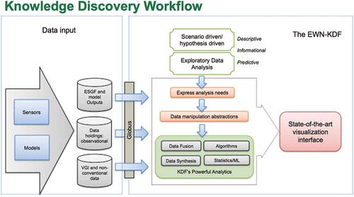
The framework (example workflow shown in Figure 5) should include 1) data content and a knowledge base, 2) an analytical toolkit and 3) a system architecture for data management. The data inventory should include the most important data sets, models, visualization tools, and decision support needs at various multimodal and multiresolution scales and the framework should enable common formats for reconciling gridded and non-gridded data, including metadata standards for geodetic and temporal indexing with cross-sectoral reconciliation. Finally, the framework should allow for defining and maintaining standards for quality control, evaluation, calibration, validation and uncertainty analyses for data and modeling.

Figure 5. Example Energy-Water Nexus Knowledge Discovery Framework Workflow. Source: Bhaduri et al. (2018).

Acknowledgments

This manuscript has been authored by employees of UT-Battelle, under contract DE-AC05-00OR22725 with the US Department of Energy. The authors would also like to acknowledge the financial and intellectual support for this research by the Integrated Assessment Research Program of the US Department of Energy’s Office of Science, Biological and Environmental Research and by the Department of Energy Office of Policy. This work is supported in part by NSF ACI-1541215.

Disclosure statement

No potential conflict of interest was reported by the authors.

Additional information

Funding

This work was supported by the Integrated Assessment Research Program of the US Department of Energy’s Office of Science; Biological and Environmental Research; Department of Energy Office of Policy; NSF ACI-1541215.

Notes

1. https://www.eia.gov/outlooks/aeo/.

2. https://www.ncdc.noaa.gov/data-access/land-based-station-data/land-based-datasets/global-historical-climatology-network-ghcn.

3. https://www.quantstart.com/articles/State-Space-Models-and-the-Kalman-Filter.

4. https://waterdata.usgs.gov/nwis/rt

5. https://www.eia.gov/electricity/monthly/epm˙table˙grapher.php?t=epmt˙1˙01˙a.

6. https://www.nrel.gov/grid/solar-power-data.html

7. https://www.eia.gov/energyexplained/?page=us˙energy˙use.

8. IHS Energy (2014), U.S. Petroleum Information/Dwights LLC Data base, PIDM 2.5: Data Management System, Englewood, Colo.

9. Statistical software: https://www.r-project.org/.

References

- Akpinar, E. K., & Akpinar, S. (2005). A statistical analysis of wind speed data used in installation of wind energy conversion systems. Energy Conversion and Management, 46(4), 515–532.
- Allen, M. R., Fernandez, S. J., Fu, J. S., & Olama, M. M. (2016). Impacts of climate change on sub-regional electricity demand and distribution in the southern united states. NatureEnergy, 1, 16103.
- Allen, M. R., Wilbanks, T. J., Preston, B. L., Kao, S.-C., & Bradbury, J. (2017). Assessing the costs and benefits of resilience investments: Tennessee valley authority case study. Technical report, Oak Ridge National Laboratory (ORNL), Oak Ridge, TN (United States). Oak Ridge Leadership Computing Facility (OLCF). https://info.ornl.gov/sites/publications/Files/Pub72433.pdf.
- Allouhi, A., El Fouih, Y., Kousksou, T., Jamil, A., Zeraouli, Y., & Mourad, Y. (2015). Energy consumption and efficiency in buildings: Current status and future trends. Journal of Cleaner Production, 109, 118–130.
- Arcaute, E., Hatna, E., Ferguson, P., Youn, H., Johansson, A., & Batty, M. (2015). Constructing cities, deconstructing scaling laws. Journal of the Royal Society Interface, 12(102), 20140745.
- Auffhammer, M., & Aroonruengsawat, A., University of California, B. (2012). Hotspots of climate-driven increases in residential electricity demand: A simulation exercise based on household level billing data for California. California Energy Commission. http://www.energy.ca.gov/2012publications/CEC-500-2012-021/CEC-500-2012-021.pdf
- Augustine, J. A., Hodges, G. B., Cornwall, C. R., Michalsky, J. J., & Medina, C. I. (2005). An update on surfradthe gcos surface radiation budget network for the continental united states. Journal of Atmospheric and Oceanic Technology, 22(10), 1460–1472.
- Aydinalp-Koksal, M., & Ugursal, V. I. (2008). Comparison of neural network, conditional demand analysis, and engineering approaches for modeling end-use energy consumption in the residential sector. Applied Energy, 85(4), 271–296.
- Ayodele, T. R., Jimoh, A. A., Munda, J. L., & Agee, J. T. (2012). Statistical analysis of wind speed and wind power potential of port elizabeth using weibull parameters. Journal of Energy in Southern Africa, 23(2), 30–38.
- Badescu, V. (1997). Verification of some very simple clear and cloudy sky models to evaluate global solar irradiance. Solar Energy, 61(4), 251–264.
- Balling, R. C., Gober, P., & Jones, N. (2008). Sensitivity of residential water consumption to variations in climate: An intraurban analysis of phoenix, arizona. Water Resources Research, 44, 10.
- Balmer, P. (2000). Operation costs and consumption of resources at nordic nutrient removal plants. Water Science and Technology, 41(9), 273–279.
- Baragona, R., & Battaglia, F. (2007). Outliers detection in multivariate time series by independent component analysis. Neural Computation, 19(7), 1962–1984.
- Barbounis, T., & Theocharis, J. B. (2007). Locally recurrent neural networks for wind speed prediction using spatial correlation. Information Sciences, 177(24), 5775–5797.
- Basalirwa, C. (1995). Delineation of uganda into climatological rainfall zones using the method of principal component analysis. International Journal of Climatology, 15(10), 1161–1177.
- Batty, M. (2013). The new science of cities. Cambridge, MA: MIT Press.
- Bauer, D. (2015). Water–energy nexus: Challenges and opportunites.
- Bay, S., Saito, K., Ueda, N., & Langley, P. (2004). A framework for discovering anomalous regimes in multivariate time-series data with local models. In Symposium on Machine Learning for Anomaly Detection, Stanford, USA.
- Bazilian, M., Rogner, H., Howells, M., Hermann, S., Arent, D., Gielen, D., … Tol, R. S. (2011). Considering the energy, water and food nexus: Towards an integrated modelling approach. Energy Policy, 39(12), 7896–7906.
- Bedacht, E., Gulev, S. K., & Macke, A. (2007). Intercomparison of global cloud cover fields over oceans from the vos observations and ncep/ncar reanalysis. International Journal of Climatology, 27(13), 1707–1719.
- Belloir, C., Stanford, C., & Soares, A. (2015). Energy benchmarking in wastewater treatment plants: The importance of site operation and layout. Environmental Technology, 36(2), 260–269.
- BERC (2017). New energy map of United States reveals disproportionate landscape of production. http://berc.berkeley.edu/new-energy-map-of-united-states-reveals-disproportionate-landscape-of-production/. Accessed 16 Nov 2017.
- Bettencourt, L. M., Lobo, J., Helbing, D., Kuhnert, C., & West, G. B. (2007a). Growth, innovation, scaling, and the pace of life in cities. Proceedings of the National Academy of Sciences, 104(17), 7301–7306.
- Bettencourt, L. M. A., & Lobo, J. (2016). Urban scaling in Europe. Journal of the Royal Society Interface, 13(116), 20160005.
- Bettencourt, L. M. A., Lobo, J., & Strumsky, D. (2007b). Invention in the city: Increasing returns to patenting as a scaling function of metropolitan size. Research Policy, 36(1), 107–120.
- Bettencourt, L. M. A., Lobo, J., Strumsky, D., & West, G. B. (2010). Urban scaling and its deviations: Revealing the structure of wealth, innovation and crime across cities. PLoS ONE, 5(11), e13541.
- Bhaduri, B. L., Simon, A., Allen, M. R., Sanyal, J., Stewart, R. N., & McManamay, R. A. (2018). Energy-water nexus knowledge discovery framework, experts meeting report. Technical report, Oak Ridge National Lab. (ORNL), Oak Ridge, TN (United States).
- Biddle, J. (2008). Explaining the spread of residential air conditioning, 1955–1980. Explorations in Economic History, 45(4), 402–423.
- Billinton, R., Chen, H., & Ghajar, R. (1996). Time-series models for reliability evaluation of power systems including wind energy. Microelectronics Reliability, 36(9), 1253–1261.
- Bodik, I., & Kubaska, M. (2013). Energy and sustainability of operation of a wastewater treatment plant. Environment Protection Engineering, 39(2), 15–24.
- Boilley, A., & Wald, L. (2015). Comparison between meteorological re-analyses from erainterim and merra and measurements of daily solar irradiation at surface. Renewable Energy, 75, 135–143.
- Bozdogan, H. (2000). Akaike’s information criterion and recent developments in information complexity. Journal of Mathematical Psychology, 44(1), 62–91.
- Breiman, L. (2001). Random forests. Machine Learning, 45(1), 5–32.
- Brelsford, C., Lobo, J., Hand, J., & Bettencourt, L. M. A. (2017). Heterogeneity and scale of sustainable development in cities. Proceedings of the National Academy of Sciences, 201606033.
- Breunig, M., Kriegel, H.-P., Ng, R., & Sander, J. (1999). Optics-of: Identifying local outliers. In European Conference on Principles of Data Mining and Knowledge Discovery (pp. 262–270). Springer, Berlin, Heidelberg.
- Breunig, M. M., Kriegel, H.-P., Ng, R. T., & Sander, J. (2000). Lof: Identifying density-based local outliers. ACM Sigmod Record, 29(2), 93–104. ACM. doi:10.1145/335191.335388
- Brown, P. D., Lopes, J. P., & Matos, M. A. (2008). Optimization of pumped storage capacity in an isolated power system with large renewable penetration. IEEE Transactions on Power Systems, 23(2), 523–531.
- Çelik, M., Dadaşer-Çelik, F., & Dokuz, A. S. (2011). Anomaly detection in temperature data using dbscan algorithm. In Innovations in Intelligent Systems and Applications (INISTA), 2011 International Symposium, 91–95. IEEE.
- Campanelli, M., Foladori, P., & Vaccari, M. (2013). Consumi elettrici ed efficienza energetica del trattamento delle acque reflue. Santarcangelo di Romagna: Maggioli editore.
- Cao, L., & Gu, Q. (2002). Dynamic support vector machines for non-stationary time series forecasting. Intelligent Data Analysis, 6(1), 67–83.
- Carle, M. V., Halpin, P. N., & Stow, C. A. (2005). Patterns of watershed urbanization and impacts on water quality. JAWRA Journal of the American Water Resources Association, 41(3), 693–708.
- Carlson, S., & Walburger, A. (2007). Energy index development for benchmarking water and wastewater utilities. Denver, CO: American Water Works Association.
- CCSP. (2007). Effects of Climate Change on Energy Production and Use in the United States. In T. J. Wilbanks, V. Bhatt, D. E. Bilello, S. R. Bull, J. Ekmann, W. C. Horak, ... M. J. Scott (Eds.), A Report by the U.S. Climate Change Science Program and the subcommittee on Global Change Research (pp. 160). Washington, DC: Department of Energy, Office of Biological & Environmental Research.
- Celik, A. N. (2004). A statistical analysis of wind power density based on the weibull and rayleigh models at the southern region of turkey. Renewable Energy, 29(4), 593–604.
- Chandola, V., Banerjee, A., & Kumar, V. (2009a). Anomaly detection: A survey. ACM Computing Surveys (CSUR), 41(3), 15.
- Chandola, V., Cheboli, D., & Kumar, V. (2009b). Detecting anomalies in a time series database. Minneapolis: Computer Science Department, University of Minnesota, Tech. Rep.
- Chang, W.-Y. (2014). A literature review of wind forecasting methods. Journal of Power and Energy Engineering, 2, 4.
- Chaudhuri, G., & Clarke, K. (2013). The sleuth land use change model: A review. Environmental Resources Research, 1(1), 88–105.
- Chawla, S., & Sun, P. (2006). Slom: A new measure for local spatial outliers. Knowledge and Information Systems, 9(4), 412–429.
- Cheng, H., Tan, P.-N., Potter, C., & Klooster, S. (2008). A robust graph-based algorithm for detection and characterization of anomalies in noisy multivariate time series. In Data Mining Workshops, 2008. ICDMW’08. IEEE International Conference on, 349–358. IEEE.
- Cheng, H., Tan, P.-N., Potter, C., & Klooster, S. (2009). Detection and characterization of anomalies in multivariate time series. In Proceedings of the 2009 SIAM International Conference on Data Mining, 413–424. SIAM.
- Choi, T., Keith, L., Hocking, E., Friedman, K., & Matheu, E. (2011). Dams and energy sectors interdependency study. Technical report, US Department of Energy and Department of Homeland Security. http://energy.gov/sites/prod/files/Dams-EnergyInterdependencyStudy.pdf.
- Clarke, K. C., Hoppen, S., & Gaydos, L. (1997). A self-modifying cellular automaton model of historical urbanization in the san francisco bay area. Environment and Planning B: Planning and Design, 24(2), 247–261.
- Cook, M. A., King, C. W., Davidson, F. T., & Webber, M. E. (2015). Assessing the impacts of droughts and heat waves at thermoelectric power plants in the united states using integrated regression, thermodynamic, and climate models. Energy Reports, 1, 193–203.
- Cutler, D. R., Edwards, T. C., Beard, K. H., Cutler, A., Hess, K. T., Gibson, J., & Lawler, J. J. (2007). Random forests for classification in ecology. Ecology, 88(11), 2783–2792.
- Dale, L. L., Dogrul, E. C., Brush, C. F., Kadir, T. N., Chung, F. I., Miller, N. L., & Vicuna, S. D. (2013). Simulating the impact of drought on californias central valley hydrology groundwater and cropping. British Journal of Environment and Climate Change, 3(3), 271–291.
- Dale, L. L., Karali, N., Millstein, D., Carnall, M., Vicuña, S., Borchers, N., … Heaps, C. (2015). An integrated assessment of water-energy and climate change in sacramento, california: How strong is the nexus? Climatic Change, 132(2), 223–235.
- Dale, V. H., Efroymson, R. A., & Kline, K. L. (2011). The land use–Climate change–Energy nexus. Landscape Ecology, 26(6), 755–773.
- Damousis, I. G., Alexiadis, M. C., Theocharis, J. B., & Dokopoulos, P. S. (2004). A fuzzy model for wind speed prediction and power generation in wind parks using spatial correlation. IEEE Transactions on Energy Conversion, 19(2), 352–361.
- Das, M., & Parthasarathy, S. (2009). Anomaly detection and spatio-temporal analysis of global climate system. In Proceedings of the third international workshop on knowledge discovery from sensor data, 142–150. ACM.
- Davis, C. (2012). The politics of fracking: Regulating natural gas drilling practices in colorado and texas. Review of Policy Research, 29(2), 177–191.
- Dieter, C. A., Maupin, M. A., Caldwell, R. R., Harris, M. A., Ivahnenko, T. I., Lovelace, J. K., … Linsey, K. S. (2018). Estimated use of water in the united states in 2015. Technical report, US Geological Survey.
- Ding, M., Zhang, L. J., & Wu, Y. C. (2005). Wind speed forecast model for wind farms based on time series analysis [j]. Electric Power Automation Equipment, 8, 32–34.
- Dyer, T. G. (1975). The assignment of rainfall stations into homogeneous groups: An application of principal component analysis. Quarterly Journal of the Royal Meteorological Society, 101(430), 1005–1013.
- Elman, J. L. (1990). Finding structure in time. Cognitive Science, 14(2), 179–211.
- Ester, M., Kriegel, H.-P., Sander, J., Xu, X. (1996). A density-based algorithm for discovering clusters in large spatial databases with noise. Kdd, 96(34), 226–231.
- Evans, L., Guthrie, G., & Videbeck, S. (2008). Assessing the integration of electricity markets using principal component analysis: Network and market structure effects. Contemporary Economic Policy, 26(1), 145–161.
- Fayyad, U., Piatetsky-Shapiro, G., & Smyth, P. (1996). From data mining to knowledge discovery in databases. AI Magazine, 17(3), 37.
- Fischer-Kowalski, M., Krausmann, F., Giljum, S., Lutter, S., Mayer, A., Bringezu, S., … Weisz, H. (2011). Methodology and indicators of economy-wide material flow accounting. Journal of Industrial Ecology, 15(6), 855–876.
- Foley, A. M., Leahy, P. G., Marvuglia, A., & McKeogh, E. J. (2012). Current methods and advances in forecasting of wind power generation. Renewable Energy, 37(1), 1–8.
- French, M. N., Krajewski, W. F., & Cuykendall, R. R. (1992). Rainfall forecasting in space and time using a neural network. Journal of Hydrology, 137(1–4), 1–31.
- Fung, A. S.-L., Aydinalp, M., & Ugursal, V. I. (1999). Econometric models for major residential energy end-uses. Halifax, Nova Scotia: CREEDAC, Dalhousie University.
- Gleick, P. H. (1994). Water and energy. Annual Review of Energy and the Environment, 19(1), 267–299.
- Goldstein, R., & Smith, W. (2002). Water & sustainability (volume 4): US electricity consumption for water supply & treatment-the next half century. Palo Alto, CA: Electric Power Research Institute.
- Gomez-Lievano, A., Patterson-Lomba, O., & Hausmann, R. (2016). Explaining the prevalence, scaling and variance of urban phenomena. Nature Human Behaviour, 1(1), s41562– 016–0012–016.
- Griffith, B., Long, N., Torcellini, P., Judkoff, R., Crawley, D., & Ryan, J. (2008). Methodology for modeling building energy performance across the commercial sector. National Renewable Energy Laboratory, Golden, CO, Technical Report NREL/TP-550-41956, March, www.nrel.gov/docs/fy08osti/41956.pdf.
- Griffiths-Sattenspiel, B., & Wilson, W. (2009). The carbon footprint of water. Portland, OR: River Network. http://el.doccentre.info/eldoc1/0905/090501zzz1B.pdf
- Haberl, H., Fischer-Kowalski, M., Krausmann, F., Weisz, H., & Winiwarter, V. (2004). Progress towards sustainability? what the conceptual framework of material and energy flow accounting (mefa) can offer. Land Use Policy, 21(3), 199–213.
- Healy, R. W., Alley, W. M., Engle, M. A., McMahon, P. B., & Bales, J. D. (2015). The water-energy nexus: An earth science perspective. Technical report, US Geological Survey.
- Helmbrecht, J., Pastor, J., & Moya, C. (2017). Smart solution to improve water-energy nexus for water supply systems. Procedia Engineering, 186, 101–109.
- Helsel, D. R., & Hirsch, R. M. (2002). Statistical methods in water resources (Vol. 49). Reston, VA: United States Geological Survey. https://pubs.usgs.gov/twri/twri4a3/pdf/twri4a3-new.pdf
- Hensley, Z., Sanyal, J., & New, J. (2014). Provenance in sensor data management. Communications of the ACM, 57(2), 55–62.
- Hervás-Martínez, C., Gutiérrez, P. A., Fernández, J. C., Salcedo-Sanz, S., Portilla-Figueras, A., Pérez-Bellido, A., & Prieto, L. (2009). Hyperbolic tangent basis function neural networks training by hybrid evolutionary programming for accurate short-term wind speed prediction. In Intelligent Systems Design and Applications, 2009. ISDA’09. Ninth International Conference on, 193–198. IEEE.
- Hirst, E. (1978). A model of residential energy use. Simulation, 30(3), 69–74.
- Hirst, E., Lin, W., & Cope, J. (1977). Residential energy use model sensitive to demographic, economic, and technological factors. Quarterly Reviews Economics Bus (United States), 17(2), 7–22.
- Hong, W.-C. (2008). Rainfall forecasting by technological machine learning models. Applied Mathematics and Computation, 200(1), 41–57.
- Hossain, M. R., Oo, A. M. T., & Ali, A. S. (2012). Hybrid prediction method of solar power using different computational intelligence algorithms. In Power Engineering Conference (AUPEC), 2012 22nd Australasian Universities, 1–6. IEEE.
- House-Peters, L., Pratt, B., & Chang, H. (2010). Effects of urban spatial structure, sociodemographics, and climate on residential water consumption in hillsboro, oregon. JAWRA Journal of the American Water Resources Association, 46(3), 461–472.
- House-Peters, L. A., & Chang, H. (2011). Urban water demand modeling: Review of concepts, methods, and organizing principles. Water Resources Research, 47(5), 1–15.
- Howells, M., Hermann, S., Welsch, M., Bazilian, M., Segerstro¨M, R., Alfstad, T., … Van Velthuizen, H. (2013). Integrated analysis of climate change, land-use, energy and water strategies. Nature Climate Change, 3(7), 621.
- Hubbert, M. K. (1949). Energy from fossil fuels. Science, 109(2823), 103–109.
- Hubbert, M. K., & Shell Development Co. (1956). Nuclear energy and the fossil fuel. In Drilling and production practice (Vol. API-56-007). New York: American Petroleum Institute.
- Hull, S. (2017). Releases at Oroville dam spillway halted due to hole. http://krcrtv.com/news/butte-county/releases-at-oroville-dam-spillway-slowed-due-to-hole
- Hunt, D. V., Leach, J. M., Lee, S., Bouch, C., Braithwaite, P., & Rogers, C. D. (2014). Material flow analysis (mfa) for liveable cities. In Proceedings of the 4th World Sustainability Forum, Vienna, Austria, 20–21.
- Ikonnikova, S., Browning, J., Horvath, S. C., Tinker, S. (2014). Well recovery, drainage area, and future drill-well inventory: Empirical study of the barnett shale gas play. SPE Reservoir Evaluation & Engineering, 17(4), 484–496.
- International Energy Agency (2014). Energy technology perspectives 2014 harnessing electricity’s potential. Technical report, Author, Paris, France.
- Jones, B., & ONeill, B. (2016). Spatially explicit global population scenarios consistent with the shared socioeconomic pathways. Environmental Research Letters, 11(8), 084003.
- Jordan, M. I. (1986). Attractor dynamics and parallellism in a connectionist sequential machine.
- Kao, S.-C., & Ganguly, A. R. (2011). Intensity, duration, and frequency of precipitation extremes under 21st-century warming scenarios. Journal of Geophysical Research: Atmospheres, 116, D16.
- Kao, S.-C., Sale, M. J., Ashfaq, M., Martinez, R. U., Kaiser, D. P., Wei, Y., & Diffenbaugh, N. S. (2015). Projecting changes in annual hydropower generation using regional runoff data: An assessment of the united states federal hydropower plants. Energy, 80, 239–250.
- Kariniotakis, G., Stavrakakis, G., & Nogaret, E. (1996). Wind power forecasting using advanced neural networks models. IEEE Transactions on Energy Conversion, 11(4), 762–767.
- Karl, T. R. (2009). Global climate change impacts in the United States. Cambridge University Press. https://nca2009.globalchange.gov.
- Kavasseri, R. G., & Seetharaman, K. (2009). Day-ahead wind speed forecasting using f-arima models. Renewable Energy, 34(5), 1388–1393.
- Kechriotis, G., Zervas, E., & Manolakos, E. S. (1994). Using recurrent neural networks for adaptive communication channel equalization. IEEE Transactions on Neural Networks, 5(2), 267–278.
- Keogh, E., Lin, J., Lee, S.-H., & Van Herle, H. (2007). Finding the most unusual time series subsequence: Algorithms and applications. Knowledge and Information Systems, 11(1), 1–27.
- Krampe, J. (2013). Energy benchmarking of south australian wwtps. Water Science and Technology, 67(9), 2059–2066.
- Labandeira, X., Labeaga Azcona, J. M., & Rodr´Iguez M´Endez, M. (2005). A residential energy demand system for spain.
- Lam, J. C., Wan, K. K., Cheung, K., & Yang, L. (2008). Principal component analysis of electricity use in office buildings. Energy and USbuildings, 40(5), 828–836.
- Lei, M., Shiyan, L., Chuanwen, J., Hongling, L., & Yan, Z. (2009). A review on the forecasting of wind speed and generated power. Renewable and Sustainable Energy Reviews, 13(4), 915–920.
- Li, G., & Shi, J. (2010). On comparing three artificial neural networks for wind speed forecasting. Applied Energy, 87(7), 2313–2320.
- Lin, G.-F., & Chen, L.-H. (2004). A non-linear rainfall-runoff model using radial basis function network. Journal of Hydrology, 289(1), 1–8.
- Longo, S., d’Antoni, B. M., Bongards, M., Chaparro, A., Cronrath, A., Fatone, F., … Hospido, A. (2016). Monitoring and diagnosis of energy consumption in wastewater treatment plants. a state of the art and proposals for improvement. Applied Energy, 179, 1251–1268.
- Luk, K., Ball, J. E., & Sharma, A. (2000). A study of optimal model lag and spatial inputs to artificial neural network for rainfall forecasting. Journal of Hydrology, 227(1), 56–65.
- Lynn, G., Luppold, W., & Kiker, C. (1979). Water responsiveness of commercial establishments. Water Resources Bulletin, 14(3), 719–729.
- Macko, P., & Seltzer, M. (2012). A general-purpose provenance library. TaPP. https://www.usenix.org/system/files/conference/tapp12/tapp12-final9.pdf
- Malla, P. B., & Gopalakrishnan, C. (1999). The economics of urban water demand: The case of industrial and commercial water use in hawaii. International Journal of Water Resources Development, 15(3), 367–374.
- Marinia, M., Palombab, C., Rizzia, P., Castia, E., Marciaa, A., & Paderib, M. (2017). A multicriteria analysis method as decision-making tool for sustainable desalination: The asinara island case study. Desalination and Water Treatment, 61, 274–283.
- Marshall, J. D. (2007). Urban land area and population growth: A new scaling relationship for metropolitan expansion. Urban Studies, 44(10), 1889–1904.
- McGranahan, G., Balk, D., & Anderson, B. (2007). The rising tide: Assessing the risks of climate change and human settlements in low elevation coastal zones. Environment and Urbanization, 19(1), 17–37.
- McKee, J. J., Rose, A. N., Bright, E. A., Huynh, T., & Bhaduri, B. L. (2015). Locally adaptive, spatially explicit projection of us population for 2030 and 2050. Proceedings of the National Academy of Sciences, 112(5), 1344–1349.
- McManamay, R. A. (2014). Quantifying and generalizing hydrologic responses to dam regulation using a statistical modeling approach. Journal of Hydrology, 519, 1278–1296.
- McManamay, R. A., Nair, S. S., DeRolph, C. R., Ruddell, B. L., Morton, A. M., Stewart, N., … Bhaduri, B. L. (2017). Us cities can manage national hydrology and biodiversity using local infrastructure policy. Proceedings of the National Academy of Sciences, page 201706201.
- Mizuta, K., & Shimada, M. (2010). Benchmarking energy consumption in municipal wastewater treatment plants in japan. Water Science and Technology, 62(10), 2256–2262.
- Mohandes, M. A., Halawani, T. O., Rehman, S., & Hussain, A. A. (2004). Support vector machines for wind speed prediction. Renewable Energy, 29(6), 939–947.
- Morton, A., Nagle, N., Piburn, J., Stewart, R. N., & McManamay, R. (2017). A hybrid dasymetric and machine learning approach to high-resolution residential electricity consumption modeling. In D. A. Griffith, Y. Chun, & D. J. Dean (Eds.), Advances in geocomputation (pp. 47–58). Switzerland: Springer.
- Morton, A., Piburn, J., McManamay, R., Nagle, N., & Stewart, R. (2016). A dasymetricbased monte carlo simulation approach to the probabilistic analysis of spatial variables. In International Conference on GIScience Short Paper Proceedings, 1.
- Munoz-Diaz, D., & Rodrigo, F. S. (2004). Spatio-temporal patterns of seasonal rainfall in spain (1912-2000) using cluster and principal component analysis: Comparison. Annales Geophysicae, 22, 1435–1448.
- Muradian, R., & Giljum, S. (2007). Physical trade flows of pollution-intensive products: Historical trends in europe and the world. In A. Hornborg, J. McNeill, & J. Martinez-Alier (Eds.), Rethinking environmental history: World-system history and global environmental change (pp. 307–323). Lanham, MD: Alta Mira Press.
- Murphy, A. H. (1996). The finley affair: A signal event in the history of forecast verification. Weather and Forecasting, 11(1), 3–20.
- National Research Council. (2010). America’s energy future: Technology and transformation. Washington, DC: National Academies Press.
- Ndiaye, D., & Gabriel, K. (2011). Principal component analysis of the electricity consumption in residential dwellings. Energy and Buildings, 43(2), 446–453.
- NIST (2017). Nist/sematech e-handbook of statistical methods.
- O’Clery, N., Gomez-Lievano, A., & Lora, E. (2016). The path to labor formality: Urban agglomeration and the emergence of complex industries. CID Working Paper 78, Center for International Development at Harvard University.
- Ogallo, L. (1989). The spatial and temporal patterns of the east african seasonal rainfall derived from principal component analysis. International Journal of Climatology, 9(2), 145–167.
- Omitaomu, O. A., Blevins, B. R., Jochem, W. C., Mays, G. T., Belles, R., Hadley, S. W., … Rose, A. N. (2012). Adapting a gis-based multicriteria decision analysis approach for evaluating new power generating sites. Applied Energy, 96, 292–301.
- Oppenheim, A. V., Schafer, R. W., & Buck, J. R. (1999). Discrete-time signal processing (2nd ed.). Upper Saddle River, NJ, USA: Prentice-Hall, Inc.
- Ortman, S. G., Cabaniss, A. H. F., Sturm, J. O., & Bettencourt, L. M. (2015). Settlement scaling and increasing returns in an ancient society. Science Advances, 1(1), e1400066– e1400066.
- Pan, T., & Wang, R. (2004). State space neural networks for short term rainfall-runoff forecasting. Journal of Hydrology, 297(1), 34–50.
- Parinet, B., Lhote, A., & Legube, B. (2004). Principal component analysis: An appropriate tool for water quality evaluation and managementapplication to a tropical lake system. Ecological Modelling, 178(3), 295–311.
- Peres, D., & Cancelliere, A. (2014). Derivation and evaluation of landslide-triggering thresholds by a monte carlo approach. Hydrology and Earth System Sciences, 18(12), 4913.
- Perrone, D., Murphy, J., & Hornberger, G. M. (2011). Gaining perspective on the waterenergy nexus at the community scale.
- Ragan, E. D., Endert, A., Sanyal, J., & Chen, J. (2016). Characterizing provenance in visualization and data analysis: An organizational framework of provenance types and purposes. IEEE Transactions on Visualization and Computer Graphics, 22(1), 31–40.
- Rahm, D. (2011). Regulating hydraulic fracturing in shale gas plays: The case of texas. Energy Policy, 39(5), 2974–2981.
- Rajagopalan, S., & Santoso, S. (2009). Wind power forecasting and error analysis using the autoregressive moving average modeling. In Power & Energy Society General Meeting, 2009. PES’09. IEEE, 1–6. IEEE.
- Ramirez, M. C. V., de Campos Velho, H. F., & Ferreira, N. J. (2005). Artificial neural network technique for rainfall forecasting applied to the sao paulo region. Journal of Hydrology, 301(1), 146–162.
- Rapson, D. (2014). Durable goods and long-run electricity demand: Evidence from air conditioner purchase behavior. Journal of Environmental Economics and Management, 68(1), 141–160. http://www.econ.ucdavis.edu/faculty/dsrapson/Rapson_LR_electricity.pdf
- Renzetti, S. (2003). Industrial and commercial water demands. In D. E. Agthe, R. B. Billings, & N. Buras (Eds.), Managing urban water supply (pp. 115–125). Dordrecht, The Netherlands: Kluwer Academic Publishers.
- Rivers, N., & Jaccard, M. (2005). Combining top-down and bottom-up approaches to energyeconomy modeling using discrete choice methods. The Energy Journal, 26(1), 83–106.
- Rodwell, E. (2002). Siting guide: site selection and evaluation criteria for an early site permit application, 1006878, final report. Electric Power Research Institute, (March 2002).
- Saaty, T. L. (1988). What is the analytic hierarchy process?. In G. Mitra, H. J. Greenberg, F. A. Lootsma, M. J. Rijckaert, & H. J. Zimmerman (Eds.), Mathematical models for decision support (pp. 109–121). Berlin: Springer.
- Saha, G., & Stephenson, J. (1980). A model of residential energy use in new zealand. Energy, 5(2), 167–175.
- Sailor, D. J., & Pavlova, A. (2003). Air conditioning market saturation and long-term response of residential cooling energy demand to climate change. Energy, 28(9), 941–951.
- Sale, M., Kao, S., Ashfaq, M., Kaiser, D., Martinez, R., Webb, C., & Wei, Y. (2011). Assessment of the effects of climate change on federal hydropower. Technical Manual, 251. https://nhaap.ornl.gov/sites/default/files/9505_FY12_Assessment_Report.pdf.
- Samaniego, H., & Moses, M. E. (2008). Cities as organisms: Allometric scaling of urban road networks. Journal of Transport and Land Use, 1(1), 21–39.
- Sanders, K. T., & Webber, M. E. (2012). Evaluating the energy consumed for water use in the united states. Environmental Research Letters, 7(3), 034034.
- SAS. (2017). Machine learning, what it is and why it matters. https://www.sas.com/en_us/insights/analytics/machine-learning.html
- Scanlon, B. R., Ruddell, B. L., Reed, P. M., Hook, R. I., Zheng, C., Tidwell, V. C., & Siebert (2017). The food-energy-water nexus: Transforming science for society. Water Resources Research, 53(5), 3550–3556.
- Schandl, H., & West, J. (2010). Resource use and resource efficiency in the asia–Pacific region. Global Environmental Change, 20(4), 636–647.
- Schleich, J., & Hillenbrand, T. (2009). Determinants of residential water demand in germany. Ecological Economics, 68(6), 1756–1769.
- Schmidt, M. (2008). The sankey diagram in energy and material flow management. Journal of Industrial Ecology, 12(1), 82–94.
- Schneider, M. L., & Whitlatch, E. E. (1991). User-specific water demand elasticities. Journal of Water Resources Planning and Management, 117(1), 52–73.
- Schütz, H., Moll, S., & Bringezu, S. (2004). Globalisation and the shifting environmental burden. In Material trade flows of the European Union. Wuppertal: Wuppertal Institute.
- Schwarzenegger, A. (2005). California’s water–energy relationship.
- Sharma, N., Sharma, P., Irwin, D., & Shenoy, P. (2011). Predicting solar generation from weather forecasts using machine learning. In Smart Grid Communications (SmartGridComm), 2011 IEEE International Conference on, 528–533. IEEE.
- Siller, T., Kost, M., & Imboden, D. (2007). Long-term energy savings and greenhouse gas emission reductions in the swiss residential sector. Energy Policy, 35(1), 529–539.
- Simon, A., & Belles, R. (2011). Estimated state-level energy flows in 2008.
- Simonovic, S. P., & Fahmy, H. (1999). A new modeling approach for water resources policy analysis. Water Resources Research, 35(1), 295–304.
- Smith, C., Belles, R., & Simon, A. (2011). Estimated water flows in 2005: United states. Technical report, Lawrence Livermore National Laboratory (LLNL), Livermore, CA.
- Solley, W. B., Pierce, R. R., & Perlman, H. A. (1998). Estimated use of water in the United States in 1995. Reston, VA: US Geological Survey.
- Spang, E., Moomaw, W., Gallagher, K., Kirshen, P., & Marks, D. (2014). The water consumption of energy production: An international comparison. Environmental Research Letters, 9(10), 105002.
- Spruston, S., Kolesov, A., & Main, D. (2012). Leveraging the energy of the group to manage the energy of the utility: The nwwbi adopts industry tools to improve energy performance. Proceedings of the Water Environment Federation, 2012(14), 2383–2402.
- Sterman, J. D. (2001). System dynamics modeling: Tools for learning in a complex world. California Management Review, 43(4), 8–25.
- Stewart, R., Piburn, J., Sorokine, A., Myers, A., Moehl, J., & White, D. (2015). World spatiotemporal analytics and mapping project (wstamp): Discovering, exploring, and mapping spatiotemporal patterns across the world’s largest open soruce data sets. ISPRS Annals of the Photogrammetry, Remote Sensing and Spatial Information Sciences, 2(4), 95.
- Stillwell, A. S., King, C. W., Webber, M. E., Duncan, I. J., & Hardberger, A. (2011). The energy-water nexus in texas. Ecology and Society, 16, 1.
- Suh, D., Kim, H., & Kim, J. (2015). Estimation of water demand in residential building using machine learning approach. In IT Convergence and Security (ICITCS), 2015 5th International Conference on, 1–2. IEEE.
- Sun, P., & Chawla, S. (2004). On local spatial outliers. In Data Mining, 2004. ICDM’04. Fourth IEEE International Conference on, 209–216. IEEE.
- Swan, L. G., & Ugursal, V. I. (2009). Modeling of end-use energy consumption in the residential sector: A review of modeling techniques. Renewable and Sustainable Energy Reviews, 13(8), 1819–1835.
- Tao, X., & Chengwen, W. (2012). Energy consumption in wastewater treatment plants in china. http://www.researchgate.net/profile/TaoXie11/publication/266146909EnergyConsumptioninWastewaterTreatmentplantsinChina/links/5428ce520cf238c6ea7cde91.pdf
- Tay, F. E., & Cao, L. (2002). Modified support vector machines in financial time series forecasting. Neurocomputing, 48(1), 847–861.
- Tian, Y., Liu, Q., Hu, Z., & Liao, Y. (2014). Wind speed forecasting based on time seriesadaptive kalman filtering algorithm. In Nondestructive Evaluation/Testing (FENDT), 2014 IEEE Far East Forum on, 315–319. IEEE.
- Tidwell, V. C., Kobos, P. H., Malczynski, L. A., Hart, W. E., & Klise, G. T. (2009). Decision support for integrated water-energy planning. Technical report, Sandia National Laboratories (SNL-NM), Albuquerque, NM (United States).
- Tinker, A., Bame, S., Burt, R., & Speed, M. (2005). Impact of non-behavioral fixed effects on water use: Weather and economic construction differences on residential water use in austin, texas. Electronic Green Journal, 1, 22.
- Tonn, B. E., & White, D. L. (1988). Residential electricity use, wood use, and indoor temperature; an econometric model. Energy Systems and Policy, 12(3), 151–165.
- Torres, J. L., Garcia, A., De Blas, M., & De Francisco, A. (2005). Forecast of hourly average wind speed with arma models in navarre (spain). Solar Energy, 79(1), 65–77.
- Tripathi, S., Srinivas, V., & Nanjundiah, R. S. (2006). Downscaling of precipitation for climate change scenarios: A support vector machine approach. Journal of Hydrology, 330(3), 621–640.
- Tso, G. K., & Yau, K. K. (2007). Predicting electricity energy consumption: A comparison of regression analysis, decision tree and neural networks. Energy, 32(9), 1761–1768.
- Tsoi, A. C., & Back, A. D. (1994). Locally recurrent globally feedforward networks: A critical review of architectures. IEEE Transactions on Neural Networks, 5(2), 229–239.
- U.S. Department of Energy (2010). Energy efficiency trends in residential and commercial buildings.
- USGS. (2017). Releases at oroville dam spillway halted due to hole. https://water.usgs.gov/software/lists/surfacewater
- Vallario, R. (2017). Climate-energy modeling and model interdependencies. Rockville, MD: Presentation at Rockville Hilton.
- Vanek, F., Albright, L. D., & Angenent, L. (2008). Energy systems engineering. New York: McGraw-Hill Professional Publishing.
- Vilanova, M. R. N., & Balestieri, J. A. P. (2014). Energy and hydraulic efficiency in conventional water supply systems. Renewable and Sustainable Energy Reviews, 30, 701–714.
- Warner, K., Ehrhart, C., Sherbinin, A. D., Adamo, S., Chai-Onn, T. (2009). In search of shelter: Mapping the effects of climate change on human migration and displacement. In In search of shelter: Mapping the effects of climate change on human migration and displacement. London: Climate Change CARE International.
- Welch, R. L., Ruffing, S. M., & Venayagamoorthy, G. K. (2009). Comparison of feedforward and feedback neural network architectures for short term wind speed prediction. In Neural Networks, 2009. IJCNN 2009. International Joint Conference on, 3335–3340. IEEE.
- Wilbanks, T. J., & Fernandez, S. (2014). Climate change and infrastructure, urban systems, and vulnerabilities: Technical report for the US Department of Energy in support of the national climate assessment. Island Press.
- Williams, M., & Suh, B. (1986). The demand for urban water by customer class. Applied Economics, 18(12), 1275–1289.
- Williams, R. J., & Zipser, D. (1989). A learning algorithm for continually running fully recurrent neural networks. Neural Computation, 1(2), 270–280.
- Worthington, A. C. (2010). Commercial and industrial water demand estimation: Theoretical and methodological guidelines for applied economics research. Estudios de Economía Aplicada, 28(2), 237–258.
- Worthington, A. C., & Hoffmann, M. (2006). A state of the art review of residential water demand modelling.
- Wu, F., & Martin, D. (2002). Urban expansion simulation of southeast england using population surface modelling and cellular automata. Environment and Planning A, 34(10), 1855–1876.
- Yang, J., Rivard, H., & Zmeureanu, R. (2005). Building energy prediction with adaptive artificial neural networks. In Ninth International IBPSA Conference, Montréal, Canada, August, 15–18.
- Yang, L., Zeng, S., Chen, J., He, M., & Yang, W. (2010). Operational energy performance assessment system of municipal wastewater treatment plants. Water Science and Technology, 62(6), 1361–1370.
- Youn, H., Bettencourt, L. M. A., Lobo, J., Strumsky, D., Samaniego, H., & West, G. B. (2016). Scaling and universality in urban economic diversification. Journal of the Royal Society Interface, 13(114), 20150937.
- Zeng, J., & Qiao, W. (2011). Support vector machine-based short-term wind power forecasting. In Power Systems Conference and Exposition (PSCE), 2011 IEEE/PES, 1–8. IEEE.
- Zhang, H. H., & Brown, D. F. (2005). Understanding urban residential water use in beijing and tianjin, china. Habitat International, 29(3), 469–491.
- Zhao, J., Lu, C.-T., & Kou, Y. (2003). Detecting region outliers in meteorological data. In Proceedings of the 11th ACM international symposium on Advances in geographic information systems, 49–55. ACM.
- Ziolkowska, J. R., & Reyes, R. (2016). Geospatial analysis of desalination in the us–An interactive tool for socio-economic evaluations and decision support. Applied Geography, 71, 115–122.