Discriminating among tectonic settings of spinel based on multiple machine learning algorithms

ABSTRACT

In geochemistry, researchers usually discriminate among tectonic settings by analyzing the chemistry elements of minerals. Previous studies have generally taken spinel and monoclinic pyroxene as subjects. Therefore, in this research, we took spinel as a breakthrough. Totally 1898 spinel samples with 14-dimension chemistry elements were collected from three different tectonic settings, including ocean island, convergent margin, and spreading center. In the experiment, 20 classification algorithms were conducted in the classification learner application of MATLAB. The validation accuracies, receiver operating characteristic curves (ROCs), and the areas under ROC curve (AUCs) show that the Bag Ensemble Classifier has the best performance in the problem. Its validation accuracy is 86.3%, and the average AUC is 0.957. For further analysis, we studied the importance of different major elements in discriminating. It has been found that TiO₂ has the best impact on discrimination, and FeO^T, Al₂O₃, Cr₂O₃, MgO, MnO, and ZnO are of less importance. Based on the Bag Ensemble Classifier, a MATLAB plug-in application named Discriminator of Spinel Tectonic Setting (DSTS) has been developed for promoting the usage of machine learning in geochemistry and facilitating other researchers to use our achievements.

KEYWORDS:

• Geochemistry
• spinel
• tectonic setting
• machine learning
• discrimination method
• application development

1. Introduction

Discrimination diagrams are always used for discriminating among different tectonic settings. In the 1970s, Pearce and Cann (1971) put forward the first discrimination diagram based on the chemistry elements of a suit of basalt samples and acquired good results. After that, more and more discrimination diagrams were designed, and they greatly enriched the theory of magmatic petrology and the geotectonic hypothesis (Pearce & Cann, 1973; Pearce & Norry, 1979; Wang et al., 2017). Like the work of Peace, the diagrams were generally designed with basalt samples and were all based on the derivation of causality (Wang, 2001; Wang et al., 2016).

Figure 9. ROC and AUC of Bag.

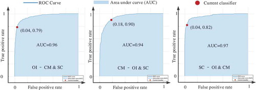
Figure 10. ROC and AUC of RUSBoost.

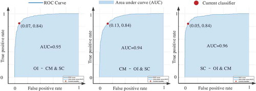
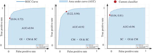
Figure 11. ROC and AUC of Weighted SVM with Gaussian kernel.

Spinel is a common kind of accessory minerals of mantle-derived xenolith. The researches of spinel can not only illustrate spinel’s characters but also reveal the genesis of its host mantle-derived rock (Arai et al., 2011). In the previous studies of using minerals to discriminating tectonic settings, spinel was often taken as the subjects (Arai, 1994; Ishwar-Kumar et al., 2016; Zhao, 2016; Zhou et al., 2011).

With the development of geochemistry, researchers find that there are many limitations in using discrimination diagrams (Li, Arndt, Tang, & Ripley, 2015; Luo et al., 2018; Zhang, 1990): (1) the samples used in the earlier discrimination diagrams were usually from a typical area, and the amount of them were small; (2) a discrimination diagram only contains 2–3 kinds of elements, which can only reflect a small amount of information; (3) the discrimination diagrams are always designed by experiments and the designing processes are subjective; and (4) oversimplifying the discrimination process goes against the in-depth study of magmatism.

With the rapid evolutions of computer techniques, machine learning algorithms begin to make its presence felt in every walk of life (Zhou et al., 2018; Zhou, Pan, Wang, & Vasilakos, 2017). Generally, machine learning can be divided into two categories: supervised learning and unsupervised learning (Ang et al., 2016). One important task can be solved by supervised learning is classification. Its main idea is to train a classifier with a set of labeled samples and then used the classifier to recognize unlabeled samples. In geochemistry, the process of discriminating among different tectonic settings is essentially a classification task. There are already some researchers who have focused on using classification algorithms to discriminate among tectonic settings. Vermeesch (2006) put forward a set of decision trees to discriminate among tectonic settings of volcanic rocks. Petrelli and Perugini (2016) proposed to use Support Vector Machines (SVM) to solve the same problem and acquire high classification scores. Ueki, Hino, and Kuwatani (2018) compared the performances of SVM, Random Forest (RF), and Sparse Multinomial Regression (SMR) algorithm in discriminating different basalt tectonic settings, pointing out that SVM and RF could reach a high accuracy and the SMR could provide more explanation. The results acquired by them show the effectiveness of intelligent algorithms in geochemistry. However, these researches were all based on basalt samples, the methods adopted in their experiments were only 1–3 of intelligent algorithms, and in the publications, the technical problems of the algorithms were not actually discussed enough. Moreover, they all just proposed a solution to discrimination, not a real tool like diagrams that can be used by others.

In this study, we focused on the using of classification algorithms in discriminating among tectonic settings, and spinel samples were taken as the subjects. To achieve a comprehensive study, 20 different classification algorithms were adopted for comparison. The result showed that the Bag Ensemble classifier had the best performance. Meanwhile, it indicates that using the chemistry of spinel to discriminate among tectonic setting is also feasible. In addition, based on our researches, a MATLAB application was developed, which can be a convenience tool for geochemistry analysis.

2. Data collection and pre-processing

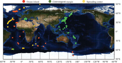
The spinel samples used in the research were obtained from the database of GEOROC (http://georoc.mpch-mainz.gwdg.de/georoc/) and PetDB (https://search.earthchem.org/). Totally 1898 pieces of spinel sample were collected. Some of them were derived from the in situ mantle, and the others are mantle rock inclusions. All the spinel samples had been labeled with their tectonic settings, and they were composed of 515 ocean island spinel (OIS) samples, 881 convergent margin spinel (CMS) samples, and 502 spreading center spinel (SCS) samples. The samples were collected from all over the world, including the Hawaiian Islands, Samoan Islands, Canary Islands, ST. Helena Chain, Tristan da Cunha Group, Galapagos Islands, Iceland, Juan Fernandez Islands, Austral-Cook Islands, Azores, Cape Verde Islands, Bouvet, Pitcairn-Gambier Chain, Caroline Islands, Marquesas, Jan Mayen, Mascarene Islands Incl. Reunion, Cameroon Line, Revillagigedo Archipelago, Trindade-Vitoria Rise, Amsterdam-ST. Paul, Balleny Islands, Hawaiian Arch Volcanic Fields, Ross Island, Crozet Islands, Scotia Arc, Aleutian Arc, Izu-Bonin Arc, Mariana Arc, Kamchatka Arc, Mariana Arc, Tonga Arc, Kurile Arc, Mariana Arc, Honshu Arc, Andean Arc, Luzon Arc, Mexican Volcanic Belts, New Hebrides Arc-Vanuatu Archipelago, Bismarck Arc-New Britain Arc, New Hebrides Arc, Central American Volcanic Arc, Aeolian Arc, New Zealand, Cascades, Yap Arc, Apenninic-Maghrebides Chain, Sulawesi Arc, Ryukyu Arc, Liguria-Sardo-Tyrrhenian Arc, Middle America Trench-Guatemala Trench, Mid-Atlantic Ridge, Southwest Indian Ridge, Galapagos Spreading Center, Parece Vela and West Philippine Basin, the Back-Arc East Scotia Ridge of South Atlantic Ocean, Juan De Fuca Ridge, and the East Pacific Rise. The distributions of them are shown in Figure 1.

Figure 1. Distribution of spinel samples.

The samples were collected by different researchers and research groups. Therefore, the test methods for the samples were different, and they were mainly detected through the fused disk X-ray fluorescence and the electron probe method. Each sample was composed of 14 kinds of major elements: SiO₂, TiO₂, Al₂O₃, Cr₂O₃, V₂O₃, Fe₂O₃, FeO, CaO, MgO, MnO, NiO, ZnO, K₂O, and Na₂O, and the unit was wt%. The types of rocks were also various, including basalt, tholeiite, diabase, andesitic, absarokite, trachy basalt, hornblende, picritic, olivine, dolerite, hawaiite, basanite, ankaramitic basalt, and nepheline. However, because the environments of the spinel samples had been clearly labeled, the rock type was not taken as a factor of our research. The data pre-processing consists of four parts: (1) for each sample, its Fe₂O₃ and FeO data were converted into FeO^T data; (2) considering that only 152/1898 samples had Na₂O data and only 134/1898 samples had K₂O data, the two major elements were not used in this experiment; (3) considering the loss of data of some samples, the samples whose total value of the major elements was less than 97 wt% were deleted. After that, there remained 1398 samples, including 366 OIS, 743 CMS, and 289 SCS.

3. Machine learning algorithms

3.1. Classification algorithms

In this study, five types of currently popular classification algorithms were adopted: Decision Trees, Discriminant Analysis, Support Vector Machines, Nearest Neighbor Classifiers, and Ensemble Classifiers. The descriptions of them are as follows:

1. Decision Trees (Gavankar & Sawarkar, 2015): The structure of a decision tree is like a tree that contains a root node, several internal nodes, and several leaf nodes. The leaf nodes correspond to classification results, and other nodes represent the tests on some attributes. According to the tests, test samples will be divided into different child nodes. Therefore, the root node contains all samples, and the route from the root node to an internal node, or child node, represents a determining sequence. Currently, there are several variants of Decision Tree. In this research, the Fine Tree, Medium Tree, Coarse Tree were adopted.

2. Discriminant Analysis (Welling, 2005): this type of classification algorithm is based on the assumption that the data of different classes obey different Gaussian distributions. The main process is firstly training a classifier to fit a function that can estimate the parameters of the distribution of each class, and then using the classifier to predict new samples. The most widely used Discriminant Analysis is the Linear Discriminant Analysis (LDA). In LDA, the key step is to find out a projection hyperplane in a k-dimensional space, then by projecting different classes of samples onto the hyperplane, maximizing the between-class distances and minimizing the within-class distances, as shown in Figure 2.

   Figure 2. Projection process of LDA.

   

   Another typical Discriminant Analysis is Quadratic Discriminant Analysis (QDA). The main difference between QDA and LDA is that a QDA is a classifier with a quadratic decision boundary. In our research, both QDA and LDA were adopted.

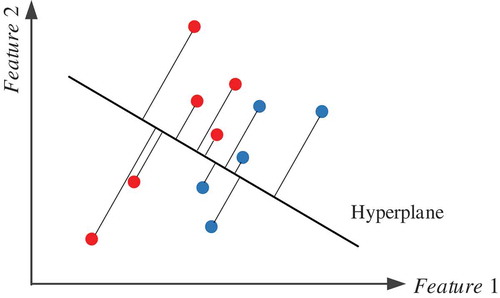
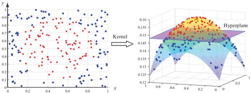
3. Support Vector Machines (SVMs) (Cortes & Vapnik, 1995; Li, Miao, & Shi, 2014): this type of algorithms are based on the theory of VC dimension and structure risk minimizing principle. The main task of SVM is to find out a hyperplane in the feature space of samples to maximize the distance between different classes, and the key of SVM is to design an effective kernel function, as shown in Figure 3. The common kernel functions include Gaussian kernel, linear kernel, quadratic kernel, and cubic kernel. In this study, all the four kernels were tried to find out which was the best one for the discrimination task.

   Figure 3. Classification process of SVM.

   

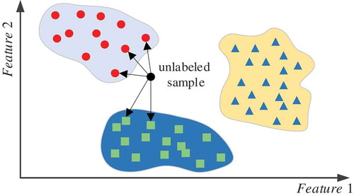
4. Nearest Neighbor Classifiers (Altman, 1992): this type of algorithms mainly includes the K-Nearest Neighbor (KNN) algorithm and its variants. KNN is one of the most simply classification algorithms. Its main idea is to find out k nearest samples of a new data in the feature space, and then classify it into a specific class according to the k neighbors, as shown in Figure 4. In this research, six Nearest Neighbor Classifiers including Fine KNN, Medium KNN, Coarse KNN, Cosine KNN, Cubic KNN, and Weighted KNN were adopted.

   Figure 4. Classification process of KNN.

   

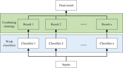
5. Ensemble Classifiers (Polikar, 2012): different from other types of classification algorithms that only contain one classifier, Ensemble Classifiers are proposed as using multiple classifiers to improve the final performance. Its strategy is to aggregate multiple weak learners into a strong learner, as shown in Figure 5. The weak learners can be Decision Trees, KNN, or other single classifiers. The main aggregation strategies include Bagging, Boosting, and Random Subspace method. In our experiment, the Bagged Trees, AdaBoosted Trees, RUSBoosted Trees, Subspace KNN, Subspace Discriminant algorithms were adopted.

   Figure 5. Basic framework of an Ensemble Classifier.

   

3.2. Assessment criteria

To assess the performance of a classifier, many criteria have been proposed. Generally, the main assessment criteria include validation accuracy, confusion matrix, receiver operating characteristic curve (ROC), and the area under the ROC curve (AUC).

1. Validation accuracy: When training a model, the whole samples will be divided into a training set and a validation set. The training set is used to determine the structure and the parameters of the classifier, and the validation set is used to test the classifier. Therefore, a good classifier has a high validation accuracy.

2. Confusion matrix: Confusion matrix is an n × n matrix that is used to visualize the performance of classifiers, where n is the number of classes. It can show the details of the classification result of a classifier by comprising the real classes and the prediction results.

3. ROC (Gönen, 2006): Considering that validation accuracy cannot really reflect the real performance of a classifier when the distribution of samples is not balanced, ROC was put forward as a new criterion. The x-axis of ROC is the false-positive rate (FPR), and the y-axis is the true-positive rate (TPR), or sensitivity, as shown in Figure 6. Generally speaking, the farther from the ROC to the reference line (red line in Figure 6), the better the performance of the classifier.

   Figure 6. Illustration of ROC and AUC.

   

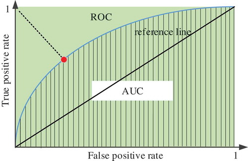
4. AUC (Swets, 1986): Although ROC can reflect the performance of a classifier intuitively, researchers always want to assess the performance with a simple number. Therefore, AUC was put forward. Just as its name implies, AUC is the area under the ROC curve. So a good classifier will have a high AUC value.

In this research, all the four criteria were used to evaluate the performances of different classifiers. The validation accuracy was first adopted to initially assess all the 20 classifiers mentioned in Section 3.1. After that, the confuse matrix, ROC, and AUC were used to assess the five classifiers that had the highest validation accuracies.

3.3. Classification learner of MATLAB

The classification learner application provided by MATLAB is a toolbox that allows users to interactively analysis data, training classifiers with several different types of machine learning algorithms, as shown in Figure 7.

Figure 7. The interface of the classification learner application of MATLAB.

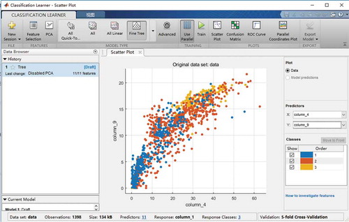
Through this application, users can select different algorithms, different features of samples, and different parameters to obtain an optimal classifier, and acquire the corresponding validation accuracy. After training, it can show the confusion matrix, ROC and AUC to the users, as well as the scatters of any two of the features of samples.

In this research, totally 20 classifiers mentioned in Section 3.1 were adopted, including Fine Tree, Medium Tree, Coarse Tree, LDA, QDA, SVM with Gaussian kernel, SVM with linear kernel, SVM with quadratic kernel, SVM with cubic kernel, Fine KNN, Coarse KNN, Cosine KNN, Cubic KNN, Weighted KNN, AdaBoost Ensemble Classifiers, Bag Ensemble Classifiers, RUSBoost Ensemble Classifiers, Subspace KNN, and Subspace Discriminant.

4. Experiment and analysis

4.1. Discrimination results

In the training process, the k-fold cross-validation method (Anguita, Ghelardoni, Ghio, Oneto, & Ridella, 2012) was adopted. In previous researches, the value of k was usually set as 10, meaning that the validation set occupies 10% of the samples. In our research, the k was set as 5 to make the validation set larger to sufficiently validate the classifiers. For each classifier, we changed the parameters manually several times to obtain the optimal parameters. The optimal parameters of different classifiers and their validation accuracy are shown in Table 1.

Table 1. Optimal parameters and validation accuracies of different classifiers.

	Classifier	Optimal parameters	Validation accuracy
Decision Trees	Fine Tree	Maximum number of splits = 150	78.20%
	Medium Tree	Maximum number of splits = 150	78.30%
	Coarse Tree	Maximum number of splits = 150	78.30%
Discriminant Analysis	LDA	Covariance structure: Full	69.00%
	QDA	Covariance structure: Full	67.70%
SVMs	SVM (Gaussian kernel)	Box constraint level = 5	84.70%
	SVM (Linear kernel)	Box constraint level = 1	73.70%
	SVM (Quadratic kernel)	Box constraint level = 3	80.90%
	SVM (Cubic kernel)	Box constraint level = 4	82.90%
Nearest Neighbor Classifiers	Fine KNN	Number of neighbors = 3	82.00%
	Medium KNN	Number of neighbors = 3	81.00%
	Coarse KNN	Number of neighbors = 3	81.60%
	Cosine KNN	Number of neighbors = 3	81.50%
	Cubic KNN	Number of neighbors = 3	82.50%
	Weighted KNN	Number of neighbors = 7–13	84.4%
Ensemble Classifiers	AdaBoost	Maximum number of splits = 100; Number of learners = 800	86.60%
	Bag	Maximum number of splits = 150; Number of learners = 1000	86.30%
	RUSBoost	Maximum number of splits = 100; Number of learners = 800	85.00%
	Subspace (Decision Tree)	Subspace dimension = 5; Number of learners = 800	80.70%
	Subspace (Discriminant)	Subspace dimension = 7; Number of learners = 800	68.00%

From Table 1, it can be seen that Ensemble classifiers and Nearest Neighbor Classifiers have better performance as a whole than the others. The five classifiers that have the highest validation accuracies are AdaBoost Ensemble Classifier (85.8%), Bag Ensemble Classifier (85.7%), RUSBoost Classifier (85.0%), SVM with Gaussian kernel (84.7%), and Weighted KNN (84.4%). After that, the ROC and AUC of the five classifiers were calculated as shown in Figures 8–12.

Figure 8. ROC and AUC of AdaBoost.

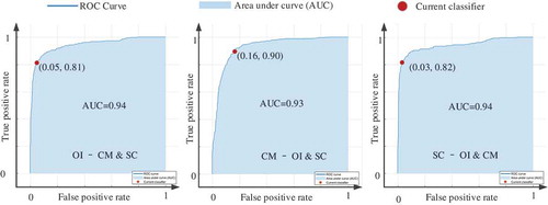
Figure 12. ROC and AUC of Weighted KNN.

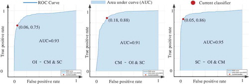
In Figures 8–12, the dark blue curves are ROCs, the light blue areas are the AUCs, and the red circles represent the status of the classifiers. For one classifier, there are three ROC curves. For example, in Figure 8, the first ROC is prediction effect of OIS and non-OIS (CMS and SCS), the second ROC reflects the prediction results of CMS and non-CMS (OIS and SCS), and the third ROC reflects the prediction results of SCS and non-SCS (OIS and CMS). Table 2 shows the AUCs of the five classifiers.

Table 2. AUCs of AdaBoost, Bag, RUSBoost, SVM with Gaussian kernel, and Weighted KNN.

Classifier	Validation accuracy	AUC (OI-CM & SC)	AUC (CM-OI & SC)	AUC (SC-OI & CM)	Average AUC
AdaBoost	86.60%	0.94	0.93	0.94	0.937
Bag	86.30%	0.96	0.94	0.97	0.957
RUSBoost	85.00%	0.95	0.94	0.96	0.950
SVM with Gaussian kernel	84.70%	0.94	0.92	0.96	0.940
Weighted KNN	84.40%	0.93	0.91	0.95	0.930
Average	85.12%	0.944	0.928	0.956	0.943

The last column of Table 2 shows that the Bag Ensemble Classifier has the highest average AUC, although it has a little less validation accuracy compared with the AdaBoost Ensemble classifier. Therefore, we took the Bag Ensemble Classifier as the best one in this experiment, and the second best is the AdaBoost. Figure 13 shows the confusion matrices of two classifiers.

Figure 13. Confusion matrix of Bag Ensemble classifier and AdaBoost Ensemble classifier.

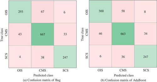
On another hand, the last row of Table 2 shows that the average AUC has the largest value at the status of SC-OI & CM, followed with OI-CM & SC and CM-OI & SC. This means that the classifiers do better in discriminating among SCS samples and non-SCS samples.

4.2. Importance of major elements

After the above assessment, we analyzed the importance of every major element. As mentioned above, the Bag Ensemble Classifier was regarded as the most suitable method. Therefore, this classifier was taken to evaluate the feature importance. In this part, 11 experiments were conducted. In each experiment, one major element was removed from the samples, and then the classifier was trained with the remaining data. For example, in the first experiment, SiO₂ data were not used for training, and the classifier was trained with the remained 10-dimension data. After training, the validation accuracy was 83.7%, and the average AUC is 0.95. The 11 results are shown in Figure 14.

Figure 14. Evaluations of the importance of major elements.

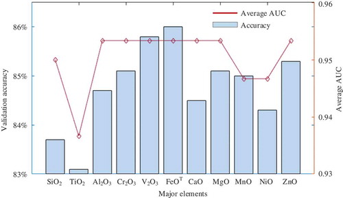
Figure 14 shows that when FeO^T, Al₂O₃, Cr₂O₃, MgO, MnO, or ZnO is not taken for training, the validation accuracy can still reach to 85%, and the average AUCs can still reach to 0.953. It means that these six major elements contribute less to discriminating among different tectonic settings. On the other hand, when TiO₂ is removed from the training samples, the validation accuracy and average AUC drop rapidly, meaning that TiO₂ contributes the most to discrimination.

4.3. Discrimination application design

From the results of Section 4.1, it can be seen that except for basalts, spinel can also be used to discriminate among different tectonic settings, and classification algorithms are effective methods for discrimination. In order to facilitate other researchers using our achievements and promote the study of machine learning in geochemistry, we developed a MATLAB application named Discriminator of Spinel Tectonic Settings (DSTS). The interface of DSTS is as Figure 15.

Figure 15. Interface of DSTS.

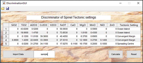
The underlying algorithm of DSTS is based on the Bag Ensemble Classifier, which has been determined as the most appropriate algorithm in Section 4.1. The main using flow is: (1) input the chemical elements into the table manually; (2) click “Calculate” button, then the application will give out the predicted tectonic settings, and show them in the last column of the table.

To improve efficiency, an “Import Data” button was designed to exchange data with the workspace of MATLAB. By inputting the name of the variable existed in the workspace into the right text box of “Import Data” button, the application can read the variable and display them on the table. Then, users can discriminate the corresponding tectonic settings by clicking the “Calculate” button.

The “Reset” button was designed to remove all the data existed in the application.

On the top of the application, there is a toolbar that contains an “Open” button and a “Save” button. The “Open” button can import excel files into MATALB, and the “Save” button is used to export the prediction results to the workspace of MATLAB.

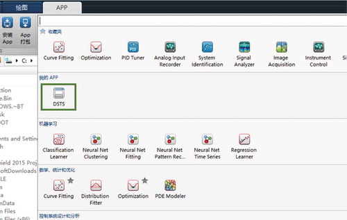
This application is now available at https://github.com/Rondapapa/DSTS/tree/dsts. The installation tutorial is in README.md. After installation, the DSTS can be found in the APP toolbox of MATLAB, as shown by the green rectangle in Figure 16.

Figure 16. Location of DSTS application.

4.4. Discussion

In the experiment, the chemical elements were all the major elements of spinel excluding Na₂O and K₂O. For each sample, the total amount was more than 97 wt%. Tables 1 and 2 show that the AdaBoost, Bag, and RUSBoost Ensemble classifier can reach a high validation accuracy of more than 85%, meaning that the 11 major elements of spinel sample can record the information of different tectonic settings. By calculating the ROCs and AUCs of the classifiers that had the highest validation accuracy, Bag Ensemble Classifiers was regarded as the most suitable algorithm for this discriminating task. By analyzing the average AUCs, it could be found that the classifiers do better in discriminating between SCS samples and non-SCS samples; the follows were discriminating between OIS samples and non-OIS sample, and the discriminating between CMS samples and non-CMS samples.

In the previous studies, spinel has been regarded as an effective indicator of the tectonic settings of basic–ultrabasic rocks. However, researchers are more inclined to use the content of Mg#, Cr#, Al₂O₃, and Fe₂O₃ for discriminating (Arai, 1994; Barnes & Roeder, 2001; Franz & Wirth, 2000; Ishwar-Kumar et al., 2016; Jan & Windley, 1990; Kamenetsky, Crawford, & Meffre, 2001; Maurel & Maurel, 1982; Oh, Seo, Choi, Rajesh, & Lee, 2012; Tamura & Arai, 2006). Only a few researchers think that TiO₂ is also a useful indicator (Dharma Rao, Santosh, Kim, & Li, 2013; Leterrier, Maury, Thonon, Girard, & Marchal, 1982). In feature analyzing of the study, it comes to a conclusion that TiO₂ had the best impact on discrimination, and FeO^T, Al₂O₃, Cr₂O₃, MgO, MnO, and ZnO were of less importance. However, the reason is not quite clear by now, and we will focus on it in the next work.

5. Conclusions

In this study, a machine learning-based analysis was carried out to discriminate among different tectonic settings with spinel samples. Totally 1898 pieces of spinel sample with 14-dimension elements were collected. After data filtering, 1398 samples with 11-dimension elements were selected for analyzing. All the spinel corresponded to three types of tectonic settings, including ocean island, convergent margin, and spreading center. The 11-dimension elements were: SiO₂, TiO₂, Al₂O₃, Cr₂O₃, V₂O₃, FeO^T, CaO, MgO, MnO, NiO, ZnO. In the experiment, totally 5 types, 20 classification algorithms were adopted for comparison, and the classification learner application provided by MATLAB was used to conduct the algorithms. The results showed that 13 classifiers can reach a high accuracy of more than 80%, and the Bag Ensemble Classifiers had the best performance on this task. Its validation accuracy was 86.3% and its average AUC was 0.957. The results prove that using spinel to discriminate among different tectonic settings is feasible, and machine learning is an effective solution for this task. In addition, the feature importance analysis proves that TiO₂ is the most important elements for discriminating, and FeO^T, Al₂O₃, Cr₂O₃, MgO, MnO, and ZnO do not have a significant impact on the performance of the classifier. And it can be a reference to further studies.

Based on these analyses, a MATLAB plug-in application was developed for the promotion of the using of machine learning in geochemistry and the convenience of other researchers using our achievements. The installation package can be downloaded from our Github repository, as well as the installation tutorial.

The shortcoming of this study is the number of spinel samples. In future work, more samples should be taken for training the classifiers. Moreover, trace elements may also contain the information about tectonic settings. As the accumulation of data, trace elements should also be taken into consideration to improve the performances of the classifiers.

Data availability statement

The data referred to in this paper are not publicly available at the current time. The DSTS application developed in this research and the installation tutorial can be downloaded from our Github repository: https://github.com/Rondapapa/DSTS/tree/dsts.

Disclosure statement

No potential conflict of interest was reported by the authors.

Additional information

Funding

This work was supported by the Tianjin Science Foundation for Distinguished Young Scientists of China [17JCJQJC44000] and the National Natural Science Foundation for Excellent Young Scientists of China [51622904].

References

- Altman, N. S. (1992). An introduction to kernel and nearest-neighbor nonparametric regression. The American Statistician, 46(3), 175–185.
- Ang, J. C., Mirzal, A., Haron, H., & Hamed, H. N. A. (2016). Supervised, unsupervised, and semi-supervised feature selection: A review on gene selection. IEEE/ACM Transactions on Computational Biology and Bioinformatics, 13(5), 971–989.
- Anguita, D., Ghelardoni, L., Ghio, A., Oneto, L., & Ridella, S. (2012). The K’in k-fold cross validation. ESANN 2012 proceedings, European Symposium on Artificial Neural Networks, Computational Intelligence and Machine Learning (pp. 441–446). Bruges, Belgium.
- Arai, S. (1994). Characterization of spinel peridotites by olivine-spinel compositional relationships: Review and interpretation. Chemical Geology, 113(3–4), 191–204.
- Arai, S., Okamura, H., Kadoshima, K., Tanaka, C., Suzuki, K., & Ishimaru, S. (2011). Chemical characteristics of chromian spinel in plutonic rocks: Implications for deep magma processes and discrimination of tectonic setting. Island Arc, 20(1), 125–137.
- Barnes, S. J., & Roeder, P. L. (2001). The range of spinel compositions in terrestrial mafic and ultramafic rocks. Journal of Petrology., 42(12), 2279–2302.
- Cortes, C., & Vapnik, V. (1995). Support-vector networks. Machine Learning, 20(3), 273–297.
- Dharma Rao, C. V., Santosh, M., Kim, S. W., & Li, S. (2013). Arc magmatism in the Delhi fold belt: Shrimp u-pb zircon ages of granitoids and implications for neoproterozoic convergent margin tectonics in nw India. Journal of Asian Earth Sciences, 78(12), 83–99.
- Franz, L., & Wirth, R. (2000). Spinel inclusions in olivine of peridotite xenoliths from TUBAF seamount (Bismarck Archipelago/Papua New Guinea): Evidence for the thermal and tectonic evolution of oceanic lithosphere. Contributions to Mineralogy and Petrology, 140, 283–295.
- Gavankar, S., & Sawarkar, S. (2015). Decision tree: Review of techniques for missing values at training, testing and compatibility. Artificial Intelligence, Modelling and Simulation (AIMS), 2015 3rd International Conference on Kota Kinabalu, State of Sabah, Island of Borneo, Malaysia.
- Gönen, M. (2006). Receiver operating characteristic (ROC) curves. SAS Users Group International, 31, 210–231.
- Ishwar-Kumar, C., Rajesh, V. J., Windley, B. F., Razakamanana, T., Itaya, T., Babu, E. V. S. S. K., & Sajeev, K. (2016). Petrogenesis and tectonic setting of the Bondla mafic-ultramafic complex, western India: Inferences from chromian spinel chemistry. Journal of Asian Earth Sciences, 130, 192–205.
- Jan, M. Q., & Windley, B. F. (1990). Chromian spinel-silicate chemistry in ultramafic rocks of the Jijal Complex, northwest Pakistan. Journal of Petrology, 31, 67–71.
- Kamenetsky, V., Crawford, A. J., & Meffre, S. (2001). Factors controlling chemistry of magmatic spinel: An empirical study of associated olivine, Cr-spinel and melt inclusions from primitive rocks. Journal of Petrology, 42, 655–671.
- Leterrier, J., Maury, R. C., Thonon, P., Girard, D., & Marchal, M. (1982). Clinopyroxene composition as a method of identification of the magmatic affinities of paleo-volcanic series. Earth and Planetary Science Letters, 59(1), 139–154.
- Li, C., Arndt, N. T., Tang, Q., & Ripley, E. M. (2015). Trace element indiscrimination diagrams. Lithos, 232, 76–83.
- Li, M. C., Miao, L., & Shi, J. (2014). Analyzing heating equipment’s operations based on measured data. Energy and Buildings, 82, 47–56.
- Luo, J. M., Wang, X. W., Song, B. T., Yang, Z. M., Zhang, Q., Zhao, Y. Q., & Liu, S. Y. (2018). Discussion on the method for quantitative classification of magmatic rocks: Taking it’s application in West Qinling of Gansu Province for example. Acta Petrologica Sinica, 34(2), 326–332.
- Maurel, C., & Maurel, P. (1982). Étude experimental de la distribution de l’aluminium entre bain silicate basique et spinel chromifère. Implications pétrogenetiques: Tenore en chrome des spinelles. Bull Minéral, 105, 197–202.
- Oh, C. W., Seo, J., Choi, S. G., Rajesh, V. J., & Lee, J. H. (2012). U-Pb SHRIMP zircon geochronology, petrogenesis, and tectonic setting of the Neoproterozoic Baekdong ultramafic rocks in the Hongseong Collision belt, South Korea. Lithos, 128(1), 100–112.
- Pearce, J., & Cann, J. (1971). Ophiolite origin investigated by discriminant analysis using Ti, Zr and Y. Earth and Planetary Science Letters, 12(3), 339–349.
- Pearce, J. A., & Cann, J. (1973). Tectonic setting of basic volcanic rocks determined using trace element analyses. Earth and Planetary Science Letters, 19(2), 290–300.
- Pearce, J. A., & Norry, M. J. (1979). Petrogenetic implications of Ti, Zr, Y, and Nb variations in volcanic rocks. Contributions to Mineralogy and Petrology, 69(1), 33–47.
- Petrelli, M., & Perugini, D. (2016). Solving petrological problems through machine learning: The study case of tectonic discrimination using geochemical and isotopic data. Contributions to Mineralogy and Petrology, 171(10), 81.
- Polikar, R. (2012). Ensemble learning. In C. Zhang & Y. Ma (Eds.), Ensemble machine learning (pp. 1–34). Springer.
- Swets, J. A. (1986). Indices of discrimination or diagnostic accuracy: Their ROCs and implied models. Psychological Bulletin, 99(1), 100–117.
- Tamura, A., & Arai, S. (2006). Harzburgite-dunite-orthopyroxenite suite as a record of supra-subduction zone setting for the Oman ophiolite mantle. Lithos, 90, 43–56.
- Ueki, K., Hino, H., & Kuwatani, T. (2018). Geochemical discrimination and characteristics of magmatic tectonic settings: A machine‐learning‐based approach. Geochemistry, Geophysics, Geosystems, 19(4), 1327–1347.
- Vermeesch, P. (2006). Tectonic discrimination of basalts with classification trees. Geochimica et Cosmochimica Acta, 70(7), 1839–1848.
- Wang, J. R., Chen, W. F., Zhang, Q., Jiao, S. T., Yang, J., Pan, Z., & Wang, S. (2017). Preliminary research on data mining of n-morb and e-morb: Discussion on method of the basalt discrimination diagrams and the character of MORB’s mantle source. Acta Petrologica Sinica, 33(3), 993–1005.
- Wang, J. R., Pan, Z. J., Zhang, Q., Chen, W. F., Yang, J., Jiao, S. T., & Wang, S. H. (2016). Intra-continental basalt data mining: The diversity of their constituents and the performance in basalt discrimination diagrams. Acta Petrologica Sinica, 32(7), 1919–1933.
- Wang, Y. (2001). Th/Hf-Ta/Hf identification of tectonic setting of basalts. Acta Petrologica Sinica, 17, 413–421.
- Welling, M. (2005). Fisher linear discriminant analysis. Department of Computer Science, University of Toronto . 3 (1)
- Zhang, Q. (1990). The correct use of the basalt discrimination diagram. Acta Petrologica Sinica, 2, 87–94.
- Zhao, Z. H. (2016). Discrimination of tectonic settings based on trace elements in igneous minerals. Geotectonica et Metallogenia, 40(5), 986–995.
- Zhou, E. B., Yang, Z. S., Jiang, W., Hou, Z. Q., Guo, F. S., & Hong, J. (2011). Study on mineralogy of Cr-spinel and genesis of Luobusha chromite deposit in South Tibet. Acta Petrologica Sinica, 27(7), 2060–2072.
- Zhou, L., Pan, S., Wang, J., & Vasilakos, A. V. (2017). Machine learning on big data: Opportunities and challenges. Neurocomputing, 237, 350–361.
- Zhou, Y. Z., Chen, S., Zhang, Q., Xiao, F., Wang, S. G., Liu, Y. P., & Jiao, S. T. (2018). Advances and prospects of big data and mathematical geoscience. Acta Petrologica Sinica, 34(2), 255–263.