Enhancing VGI application semantics by accounting for spatial bias

ABSTRACT

Volunteered geographic information (VGI) is becoming an important source of geospatial big data that support many applications. The application semantics of VGI, i.e. how well VGI reflects the real-world geographic phenomena of interest to the application, is essential for any VGI applications. VGI observations often are spatially biased (e.g. spatially clustered). Spatial bias poses challenges on VGI application semantics because it may impede the quality of inferences made from VGI. Using species distribution modeling (SDM) as an example application, this article argues that spatial bias impedes VGI application semantics, as gauged by SDM model performance, and accounting for bias enhances application semantics. VGI observations from eBird were used in a case study for modeling the distribution of the American Robin (Turdus migratorius) in U.S. T. migratorius observations from the North American Breeding Bird Survey were used as independent validation data for model performance evaluation. A grid-based strategy was adopted to filter eBird species observations to reduce spatial bias. Evaluations show that spatial bias in species observations degrades SDM model performance and filtering species observations improves model performance. This study demonstrates that VGI application semantics can be enhanced by accounting for the spatial bias in VGI observations.

KEYWORDS:

• Volunteered geographic information (VGI)
• application semantics
• spatial bias
• species distribution modeling (SDM)

1. Introduction

With the rapid development and popularization of enabling technologies (e.g. smart phones that are location-aware and interconnected to the Internet), average citizens nowadays are actively contributing voluminous geo-referenced observations of geographic phenomena around the world (See et al., 2016). Such geographic information was termed “volunteered geographic information” (VGI) (Goodchild, 2007). VGI broadly encompasses geographic information created through public participatory geographic information systems, citizen science, crowdsourcing, and social media, amongst other mechanisms; VGI has been revolutionizing the way geographic data, information, and knowledge are generated and disseminated (Sui, Elwood, & Goodchild, 2013). Moreover, VGI is an important source of geospatial big data that could potentially shift geographic research to a new “data-intensive” or “data-driven” paradigm (Kelling et al., 2009; Miller & Goodchild, 2014).

There are a wide range of VGI applications. Examples include mapping streets and roads across the globe (Haklay & Weber, 2008), documenting bird species around the world (Sullivan et al., 2009), mapping wildlife habitat (Zhu et al., 2015; Zhang et al., 2018), mapping and validating land use/cover (Fonte, Bastin, See, Foody, & Lupia, 2015; Arsanjani, Jamal, Bakillah, Hagenauer, & Zipf, 2013), supporting disaster relief (Zook, Graham, Shelton, & Gorman, 2010), studying human mobility patterns (Huang & Wong, 2015), etc.

For any meaningful VGI application, understanding the data semantics and application semantics of VGI is essential. Various definitions have been proposed for the notion of data semantics. For example, data semantics is defined as the “meaning and the use of data” (Wood, 1985), or as the “meaning of data” and “a reflection of the real world” (Sheth, 1997). Moreover, there is a distinction between “data application semantics” and “data semantics”, emphasizing that applications provide the context of the use of data (Sheth, 1997). It is thus important, for any VGI application, to fully understand the meaning of VGI observations and, more importantly, how well these VGI observations reflect the interested spatiotemporal dynamics of geographic phenomena in the real world.

Understanding the meaning of VGI observations falls within the extent of geospatial semantics (Kuhn, 2005). Geospatial semantics is the foundation and enabler of geospatial semantic web (Egenhofer, 2002), linked spatiotemporal data (Janowicz, Scheider, Pehle, & Hart, 2012), spatial data infrastructure and sharing (Janowicz et al., 2010; Zhang, Li, & Zhao, 2007), geospatial semantic search (Li, Goodchild, & Raskin, 2014), automatic composition of geospatial web service chains (Yue, Liping, Yang, Genong, & Zhao, 2007), etc. The meaning of VGI observations (i.e. what they are) is often clear and can be easily represented. For example, the meaning of VGI observations regarding a bird species is simply the occurrence time/locations of the bird. Such data semantics can be used to share, search, link the VGI dataset to other relevant data, or even automatically compose the VGI dataset an input to a species distribution modeling (SDM) web service to generate a distribution map of the bird species.

However, assessing the application semantics of VGI observations in terms of their ability to reflect the real-world geographic phenomena is more challenging. Unlike geographic samples collected following well designed spatial sampling scheme such as stratified random sampling (Jensen & Shumway, 2010), VGI observations are usually accumulated in an “opportunistic” manner (Zhu et al., 2015). That is, individual VGI contributor decides where to carry out observation at their own will without following a coordinated sampling plan. As a result, the spatial distribution of VGI observations is often biased. For example, most VGI observations tend to cluster in certain geographic areas such as cities and their vicinities, or areas with better accessibility (Zhang & Zhu, 2019). Or, the density of VGI observations differs across different areas (Beck, Böller, Erhardt, & Schwanghart, 2014) simply because some areas are more interesting to the observers. The implication is that the spatial distribution of the geographic phenomenon of interest to the application cannot be accurately inferred from the VGI observations (i.e. a spatially biased geographic sample) (Kadmon, Farber, & Danin, 2004). For instance, SDM requires species data that adequately represent the habitat use of the species (Franklin & Miller, 2009). Ideally, such species data should be collected following rigorous spatial sampling such as line transect sampling (Anderson, Laake, Crain, & Burnham, 1979) with a balanced spatial coverage of the study area. Yet volunteer-contributed species observations are subject to spatial bias and therefore may not meet the requirement of SDM. Spatial bias thus degrades the application semantics of VGI. The spatial bias in VGI observations need to be accounted for to enhance VGI application semantics.

This study argues that the spatial bias in VGI observations, spatial clustering in particular, adversely affects VGI application semantics and that accounting for the spatial bias can enhance VGI application semantics. Data from the eBird citizen science project (Sullivan et al., 2014) were used as an example of VGI. Spatial bias in the eBird data was investigated by comparing eBird data against the data from the North American Breeding Bird Survey (BBS), which can be conceived as being resulted from a stratified random sampling design (Robbins, Bystrak, & Geissler, 1986). Moreover, occurrence locations of the American Robin (Turdus migratorius) extracted from the eBird data were used for SDM. As a comparison, spatial bias in the occurrence data was reduced using a grid-based strategy. Performance of the model trained using the bias-reduced occurrences was compared to that of the model trained using the biased occurrences to examine whether accounting for spatial bias improves model performance (i.e. enhancing VGI application semantics).

2. Materials and methods

2.1. ebird data

2.1.1. Checklist locations

eBird data are freely available at www.ebird.org. eBird checklists represent sampling events, each containing information of a bird watching activity (e.g. geographic location, locality type, time, observer, observation protocol type, etc.) and the observed count or presence of bird species (Munson et al., 2012). Checklist locations within the contiguous U.S. were filtered by time, protocol type, and locality type. Records in June 2012 (matching the timeframe of the BBS data; see next section), with protocol types “stationary count” and “casual observation” and locality types “plot specific locations on a map” and “choose existing locations from a map” were selected from the eBird database. Filtering by protocol type and locality type intended to reduce positional uncertainty in the checklist locations. After removing duplicate locations, a set of 31767 checklist locations remained (Figure 1). Obviously, the checklist locations tend to cluster in populous regions in the contiguous U.S., such as the northeast, the west coast, and the vicinity of large cities in the mid-west. These locations represent the spatial pattern of observation efforts of the birders.

Figure 1. eBird checklist locations and occurrence locations of T. migratorius in June 2012.

2.1.2. Species occurrence locations

T. migratorius was reported at 8929 of the selected checklist locations (Figure 1). The occurrences were reviewed and approved by regional experts (Sullivan et al., 2009). T. migratorius was selected as the target species in this study because it is a migratory bird that is widely distributed throughout North America (Dewey & Middleton, 2002). Due to the biased spatial distribution of the checklist locations, the T. migratorius occurrence locations are also biased toward populous regions. It is more likely an artefact of the spatial bias in the observation efforts (as represented by the checklist locations) instead of a reflection of the true distribution of the species. These occurrence locations were used to training species distribution models to predict the geographic distribution of the species.

2.2. BBS data

2.2.1. BBS routes

The BBS project has been monitoring the status and trends of bird populations in North America since 1966 (Wikipedia, 2016). The BBS routes are 24.5 miles long and there are 50 stops at every 0.5 mile (800 m) along the route. The surveys take place during the peak of the nesting season, that is, June (or May in countries with warmer temperatures). At each stop, the observer records on prepared forms the total number of each bird species heard and seen within a radius of 0.25 mile (400 m). BBS routes are distributed following a stratified random design to ensure roughly uniform spatial coverage and to sample habitats representative of the entire region (Pardieck, Ziolkowski, Hudson, & Campbell, 2016; Robbins et al., 1986; Sauer et al., 2013). BBS 2012 survey data (Pardieck, Ziolkowski, Lutmerding, & Hudson, 2018) were downloaded from www.pwrc.usgs.gov/bbs/rawdata. Figure 2 shows the first stops of active 2012 BBS routes in the contiguous U.S. (3360 routes). These stop locations represent spatially balanced observation efforts of the surveyors, and thus they were used as a benchmark to assess spatial bias in the eBird checklist locations.

Figure 2. BBS routes and occurrence locations of T. migratorius in June 2012.

2.2.2. Species occurrence locations

Occurrences of T. migratorius were recorded on 1735 routes surveyed in June 2012. The species was recorded at multiple stops on each of the routes as it is a common species in North America. To avoid spatial clustering of occurrence locations along the routes, only one stop on each route was randomly selected as species occurrence location. Due to the stratified random design of the routes, the results of the bird survey along these routes are thus regarded as representative of the true distribution of bird species. Thus, these occurrence locations of T. migratorius (Figure 2) were used as validation data to evaluate the performance of species distribution models training using the species occurrence data extracted from eBird.

2.3. Environmental data

A set of 5 environmental variables representing terrain condition, landscape configuration, climatic variations, and human activity impact were used for modeling the geographic distribution of T. migratorius: elevation, land cover type, average temperature and precipitation in June, and population density. These variables are recommended by the eBird project for modeling bird distributions (Munson et al., 2012). Elevation data and land cover type data were downloaded from www.earthenv.org (Amatulli et al., 2018). Data for the two climatic variables were downloaded from worldclim.org (Fick & Hijmans, 2017). Population density data (Columbia University 2018) were obtained through earthdata.nasa.gov. All environmental data layers were in raster format at a spatial resolution of 1 km.

2.4. Point pattern analysis

To identify the spatial clustering (i.e. spatial bias) in the “opportunistic” eBird checklist locations, point pattern of the checklist locations was compared to the pattern of the stratified-random-design BBS routes using Ripley’s K function (Ripley, 1976) and kernel density estimation (KDE) (Brunsdon, 1995).

2.4.1. Ripley’s K function

Ripley’s K function is a widely used point pattern analysis method; It is defined as (Ripley, 1976):

(1) $K\left(h\right)=\frac{1}{\lambda }E\left(h\right)$(1)

where λ is the intensity of points and E(h) is the expected number of points within distance h. In practice, K function is estimated by:

(2) $K\left(h\right)=\frac{A}{n\cdot n}\sum {\sum }_{i\ne j}\frac{I_h\left(d_{ij}\right)}{w_{ij}}$(2)

where A is the area of the study area; n is the total number of points; d_ij is the distance between points i and point j; I_h(d_ij) = 1 if d_ij ≤ h, otherwise I_h(d_ij) = 0; w_ij is an edge effect correction weight. If a point pattern follows the property of complete spatial randomness (CSR) at the spatial scale h, $K\left(h\right)$ is expected to be πh². Equivalently, one can examine the corresponding L function:

(3) $L\left(h\right)=\sqrt{K\left(h\right)/\pi }$(3)

A point pattern is CSR at spatial scale h if $L\left(h\right)$ = h, clustered if $L\left(h\right)$ > h, and dispersed if $L\left(h\right)$ < h.

For statistical significance test, the points were repeatedly randomly resampled with replacement to generate bootstrap samples (e.g. 100 bootstrap samples). $L\left(h\right)$ is estimated on each bootstrap sample and confidence intervals of $L\left(h\right)$are then compared to h to determine whether the observed point pattern is statistically significantly different from CSR (i.e. whether $L\left(h\right)$ is statistically significantly different from h).

The K function implementation proposed by Zhang, Huang, Zhu, and Keel (2016) that enables K function estimation on a large number of points was adopted for analysing point patterns of the eBird checklist locations and the first stop locations of the BBS routes.

2.4.2. Kernel density estimation

KDE is a classical approach to spatial point pattern analysis that identified interesting “hotspots” of point events. KDE assumes that an event occurred at a given location X_i could occur at another location x at a probability that is inversely related to the distance from X_i to x. KDE estimates the occurrence probability density at any location x by summing up density contribution from all sample points (Brunsdon, 1995):

(4) $f\left(x\right)=\frac{1}{n}{\sum }_{i=1}^n\frac{1}{h^2}K\left(\frac{\left|x-X_i\right|}{h}\right)$(4)

where $f\left(x\right)$ is the estimated density at location $x$, h the bandwidth, $n$ the total number of sample points, and $K\left(\cdot \right)$ a kernel function.

The KDE algorithm with cross-validated optimal bandwidth based on the maximum likelihood principle (Zhang, Zhu, & Huang, 2017) was adopted for estimating probability density surfaces from the eBird checklist locations, the first stop locations of the BBS routes, T. migratorius occurrence locations from eBird, and T. migratorius occurrence locations from BBS to identify any spatial clustering (i.e. spatial bias) in the observation efforts and in the species occurrence locations.

2.5. Species distribution modeling

T. migratorius occurrence locations extracted from eBird were used for modeling the geographic distribution of the species using the Maxent method (Phillips, Anderson, & Schapire, 2006). Using model performance as an indication of application semantics, it investigates the adverse impacts of spatial bias on VGI application semantics.

2.5.1. Maxent

Maxent is the state-of-the-art SDM method which models species distribution from species presence-only data (Phillips et al., 2006). It generally performs better than other modeling methods (Elith et al., 2006). Maxent can take categorical and continuous environmental variables as predictors and make good predictions even on small-size samples (Phillips et al., 2006; Phillips & Dudík, 2008). The default parameter values of the Maxent software were fine-tuned using a large data set and thus users do not need to spend much effort on tuning model parameters (Phillips & Dudík, 2008). Thus, the recommended default values of Maxent software (version 3.4.0; biodiversityinformatics.amnh.org/open_source/maxent/) were used for SDM in this study.

2.5.2. Model performance evaluation

T. migratorius occurrence locations extracted from the BBS data were used as validation data to evaluate model performance. The area under the curve (AUC) was adopted as an accuracy measure of SDM model performance. AUC can be computed for a predicted distribution probability map based on the BBS T. migratorius occurrence locations and background locations chosen uniformly at random from the study area (Phillips & Dudík, 2008). The AUC is the probability that the predicted occurrence probability at a randomly chosen occurrence location will be higher than that at a randomly chosen background location (Phillips et al., 2006). The AUC ranges from 0.5 to 1, with AUC = 0.5 indicating random predictions and AUC = 1 indicating perfect prediction.

3. Accounting for spatial bias

A grid-based spatial filtering strategy (Boria, Olson, Goodman, & Anderson, 2014) was adopted to filter the eBird species occurrences to reduce spatial bias. A grid consisting of 50 km × 50 km squares was overlaid with the eBird T. migratorius occurrence locations over study area (contiguous U.S.) and only one species occurrence location was randomly selected within each square. Sampling by this filtering strategy resulted in 1311 T. migratorius occurrence locations (Figure 3) (out of the original 8929 occurrence locations). Spatial clustering of the original eBird T. migratorius occurrences was greatly reduced. These filtered species occurrences were used for SDM.

Figure 3. T. migratorius occurrence locations (eBird) filtered using a 50 km × 50 km grid.

Performance of the SDM model trained using the filtered species occurrences (bias reduced) was compared to that of the model trained using the original occurrences (biased) to examine whether accounting for spatial bias improves model performance (i.e. enhance VGI application semantics).

4. Results

4.1. Spatial bias in VGI observations

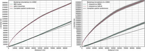
The spatial point pattern of the eBird checklist locations were heavily clustered at all spatial scales examined, whereas BBS routes was close to a complete spatial randomness at spatial scales (distance h) less than 50 km (Figure 4). It suggests that the observation efforts as represented by the eBird checklist locations were spatially clustered (i.e. biased), whilst there was not much spatial bias in the observation efforts of BBS surveyors. Unsurprisingly, T. migratorius occurrence locations from eBird were also spatially biased at all spatial scales examined, whereas the spatial point pattern of T. migratorius occurrence locations from BBS approximates a CSR at spatial scales less than 30 km. The spatial bias in the eBird T. migratorius occurrences was a result of the spatial bias in the eBird observation efforts.

Figure 4. L functions of the observation efforts and the T. migratorius occurrence locations.

The probability density surfaces estimated using KDE based on the eBird checklist locations and T. migratorius occurrence locations (eBird) showed a similar spatial pattern that closely resembles the spatial pattern of population density distribution (Columbia University 2018) (Figure 5). The areas with high probability densities are essentially large population canters. This again attests the observation that eBird observation efforts were subject to spatial bias, and it led to spatial bias in the T. migratorius occurrence locations extracted from eBird. The density surfaces estimated based on the BBS routes and T. migratorius occurrence locations also showed a similar spatial pattern with a high-density region in the northeast, indicating certain degree of spatial bias toward the populous region. Nonetheless, the magnitude of bias in the BBS data was much less significant compare to that in the eBird data.

Figure 5. Probability density surfaces of the observation efforts and the T. migratorius occurrence locations.

4.2. VGI application semantics enhancement

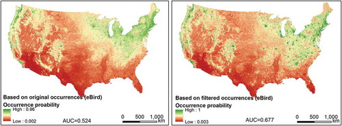
Reducing spatial bias in the eBird T. migratorius occurrence locations using the grid-based spatial filtering strategy improved SDM performance (Figure 6). Using the original unfiltered species occurrence for SDM, the model performance (AUC = 0.524) was not much better than that of a random model (AUC = 0.5). In contrast, AUC of SDM using the filtered species occurrences increased to 0.677. That is, the probability that the predicted occurrence probability at a randomly chosen BBS T. migratorius occurrence location being higher than that at a randomly chosen background location has improved from 52.4% to 67.7%.

Figure 6. Distribution maps of the T. migratorius predicted using Maxent based on the original occurrences and the filtered occurrences.

5. Discussion

5.1. Spatial bias and VGI application semantics

The performance of SDM using the spatially biased eBird T. migratorius occurrence locations resulted from the biased observation efforts was poor (AUC = 0.524). It indicates that the application semantics of the eBird data for SDM applications was weakened by spatial bias. It confirms that spatial bias in VGI observations would impede VGI application semantics.

The grid-based spatial filtering strategy randomly samples eBird T. migratorius occurrence locations with a minimum distance of 50 km between the sampled locations. This strategy effectively rarefies the original occurrence locations and thus reduces spatial bias (spatial clustering). The performance of SDM using the filtered eBird T. migratorius occurrence locations (AUC = 0.677) was significantly improved compared to SDM performance using the original occurrence locations. It indicates that the filtering strategy can effectively reduce spatial bias in VGI observations to enhance VGI application semantics.

5.2. Impact of filtering grid size

The size of the filtering grid determines the minimum distance between the filtered eBird T. migratorius occurrence locations. The filtered occurrences would generally be further away from each other as the grid size increases. Thus, the spatial bias in the species occurrences would be reduced more significantly. A larger grid size would also result in fewer squares over the study area and therefore a smaller number of occurrences will be sampled (because only one occurrence is sampled from each square). As a result, the filtering grid size may have an impact on the performance of SDM using the filtered species occurrences.

The grid-based spatial filtering strategy was applied on the eBird T. migratorius occurrence locations with grid sizes from 5 km × 5 km through 100 km × 100 km. The filtered species occurrences were then used for SDM to examine the impact of the filtering grid size on SDM performance. Results revealed that SDM performance using filtered species occurrences (AUC ≥ 0.568) was better than SDM performance using the original occurrences (AUC = 0.524) and SDM performance improved with increasing grid size although the sample size was reduced (AUC = 0.680 with a grid size of 100 km and a sample size of 555) (Table 1). It again suggests that the grid-based spatial filtering strategy was effective to reduce spatial bias in VGI observations to enhance VGI application semantics; The application semantics can be better enhanced with more spatial bias reduced.

Table 1. Impact of the filtering grid size on SDM model performance.

Grid size	5 km	10 km	20 km	50 km	100 km
Sample size	5469	4205	2848	1285	555
AUC	0.568	0.598	0.632	0.677	0.680

6. Conclusion

This article argues that the spatial bias in VGI observations impedes the application semantics of VGI and that accounting for spatial bias can enhances VGI application semantics. Species distribution modeling was adopted as an example of VGI application in this study. A case study of using VGI observations from eBird for modeling T. migratorius distribution in the contiguous U.S. demonstrates that spatial bias in VGI observations degrades SDM model performance (i.e. impeding VGI application semantics); Accounting for spatial bias by spatial filtering species observations improves SDM performance (i.e. enhancing VGI application semantics).

VGI is becoming an increasingly important source of geographic information that could be useful for many applications. However, data quality issues of VGI are widely acknowledged (Goodchild & Li, 2012). Spatial bias is one of the issues that may hinder the application semantics of VGI (Zhang & Zhu, 2018). Spatial bias or other data quality issues thus need to be properly accounted for in VGI applications in order to improve the quality of inferences made from VGI (i.e. to enhance application semantics) (Zhu et al., 2015; Zhang & Zhu, 2019). This study advocates the full use of VGI for applications and showcases VGI application semantics enhancement by accommodating its data quality issues.

Data availability statement

The data referred to in this paper is not publicly available at the current time.

Disclosure statement

No potential conflict of interest was reported by the author.

Additional information

Funding

The work reported here was supported by the Faculty Research Fund [grant number 84363-145015] and the Faculty Startup Fund at the University of Denver.

References

- Amatulli, G., Domisch, S., Tuanmu, M.-N., Parmentier, B., Ranipeta, A., Malczyk, J., & Jetz, W. (2018). A suite of global, cross-scale topographic variables for environmental and biodiversity modeling. Scientific Data, 5, 180040.
- Anderson, D. R., Laake, J. L., Crain, B. R., & Burnham, K. P. (1979). Guidelines for line transect sampling of biological populations. The Journal of Wildlife Management, 43(1), JSTOR: 70–78.
- Arsanjani, J., Jamal, M. H., Bakillah, M., Hagenauer, J., & Zipf, A. (2013). Toward mapping land-use patterns from volunteered geographic information. International Journal of Geographical Information Science, 27(12), 2264–2278.
- Beck, J., Böller, M., Erhardt, A., & Schwanghart, W. (2014). Spatial bias in the GBIF database and its effect on modeling species geographic distributions. Ecological Informatics, 19, 10–15.
- Boria, R. A., Olson, L. E., Goodman, S. M., & Anderson, R. P. (2014). Spatial filtering to reduce sampling bias can improve the performance of ecological niche models. Ecological Modelling, 275, 73–77.
- Brunsdon, C. (1995). Estimating probability surfaces for geographical point data: An adaptive kernel algorithm. Computers & Geosciences, 21(7), 877–894.
- Columbia University, Center for International Earth Science Information Network - CIESIN. (2018). Gridded population of the world, Version 4 (GPWv4): Population density, revision 11. Palisades, NY: NASA Socioeconomic Data and Applications Center (SEDAC).
- Dewey, T., & Middleton, C. (2002). Turdus Migratorius. Animal Diversity Web. Retrieved from https://animaldiversity.org/accounts/Turdus_migratorius/
- Egenhofer, M. J. (2002). Toward the semantic geospatial web. Proceedings of the 10th ACM International Symposium on Advances in Geographic Information Systems (pp. 1–4). McLean, Virginia: ACM.
- Elith, J., Graham, C. H., Anderson, R. P., Dudík, M., Ferrier, S., Guisan, A., … Zimmermann, N. (2006). Novel methods improve prediction of species’ distributions from occurrence data. Ecography, 29(2), 129–151.
- Fick, S., & Hijmans, R. (2017). WorldClim 2: New 1 Km Spatial resolution climate surfaces for global land areas. International Journal of Climatology, 37(12), 4302–4315.
- Fonte, C. C., Bastin, L., See, L., Foody, G., & Lupia, F. (2015). Usability of VGI for validation of land cover maps. International Journal of Geographical Information Science, 29(7), 1269–1291.
- Franklin, J., & Miller, J. A. (2009). Mapping species distributions: Spatial inference and prediction (Vol. 338). Cambridge: Cambridge University Press.
- Goodchild, M. F. (2007). Citizens as sensors: The world of volunteered geography. Geojournal, 69(4), 211–221.
- Goodchild, M. F., & Li, L. (2012). Assuring the quality of volunteered geographic information. Spatial Statistics, 1, 110–120.
- Haklay, M., & Weber, P. (2008). OpenStreetMap: User-generated street maps. Pervasive Computing, IEEE, 7(4), 12–18.
- Huang, Q., & Wong, D. W. S. (2015). Modeling and visualizing regular human mobility patterns with uncertainty: An example using twitter data. Annals of the Association of American Geographers, 105(6), 1179–1197.
- Janowicz, K., Schade, S., Bröring, A., Keßler, C., Maué, P., & Stasch, C. (2010). Semantic enablement for spatial data infrastructures. Transactions in GIS, 14(2), 111–129.
- Janowicz, K., Scheider, S., Pehle, T., & Hart, G. (2012). Geospatial semantics and linked spatiotemporal data-past, present, and future. Semantic Web, 3(4), 321–332.
- Jensen, R. R., & Shumway, J. M. (2010). Sampling our world. In B. Gomez & J. Paul Jones III (Eds.), Research methods in geography: A critical introduction (pp. 77–90). John Wiley & Sons.
- Kadmon, R., Farber, O., & Danin, A. (2004). Effect of roadside bias on the accuracy of predictive maps produced by bioclimatic models. Ecological Applications, 14(2), 401–413.
- Kelling, S., Hochachka, W. M., Fink, D., Riedewald, M., Caruana, R., Ballard, G., & Hooker, G. (2009). Data-intensive science: A new paradigm for biodiversity studies. Bioscience, 59(7), 613–620.
- Kuhn, W. (2005). Geospatial semantics: Why, of What, and How? Journal on Data Semantics, III, 1–24. Springer.
- Li, W., Goodchild, M. F., & Raskin, R. (2014). Towards geospatial semantic search: exploiting latent semantic relations in geospatial data. International Journal of Digital Earth, 7(1), 17–37.
- Miller, H. J., & Goodchild, M. F. (2014). Data-driven geography. GeoJournal, 80(4), 449–461.
- Munson, A. M., Webb, K., Sheldon, D., Fink, D., Hochachka, W. M., Iliff, M., … Kelling, S. (2012). The ebird reference dataset, version 4.0 (pp. 1–11). Ithaca, NY: Cornell Lab of Ornithology and National Audubon Society.
- Pardieck, K. L., Ziolkowski, D. J., Jr, Hudson, M.-A. R., & Campbell, K. (2016). North American Breeding Bird Survey Dataset 1966–2015, Version 2015.1. doi:10.5066/F7C53HZN
- Pardieck, K. L., Ziolkowski, D. J., Jr, Lutmerding, M., & Hudson, M.-A. R. (2018). North American breeding bird survey dataset 1966–2017, version 2017.0. U.S. Geological Survey, Patuxent Wildlife Research Center. doi:10.5066/F76972V8
- Phillips, S. J., Anderson, R. P., & Schapire, R. E. (2006). Maximum entropy modeling of species geographic distributions. Ecological Modelling, 190(3–4), 231–259.
- Phillips, S. J., & Dudík, M. (2008). Modeling of species distributions with maxent: New extensions and a comprehensive evaluation. Ecography, 31(2), 161–175.
- Ripley, B. D. (1976). The second-order analysis of stationary point processes. Journal of Applied Probability, 13(2), 255–266.
- Robbins, C. S., Bystrak, D., & Geissler, P. H. (1986). The breeding bird survey: Its first fifteen Years, 1965–1979 (No. FWS-PUB-157). Patuxent wildlife research center (Vol. 89). Laurel, MD: DTIC Document. doi:10.2307/1368666
- Sauer, J. R., Hines, J. E., Fallon, J. E., Link, W. A., Fallon, J. E., Pardieck, K. L., & Ziolkowski, D. J. (2013). The north american breeding bird survey 1966–2011: Summary analysis and species accounts. North American Fauna, 79(79), 1–32.
- See, L., Mooney, P., Foody, G., Bastin, L., Comber, A., Estima, J., … Rutzinger, M. (2016). Crowdsourcing, citizen science or volunteered geographic information? The current state of crowdsourced geographic information. ISPRS International Journal of Geo-Information, 5(5), 55.
- Sheth, A. (1997). Panel: Data semantics: What, where and how? Database Applications Semantics: Proceedings of the IFIP WG 2.6 Working Conference on Database Applications Semantics (DS-6) Stone Mountain (pp. 601–610), Atlanta, Georgia, U.S.A., May 30 - June 2, 1995: Springer.
- Sui, D., Elwood, S., & Goodchild, M. (eds). (2013). Crowdsourcing geographic knowledge: Volunteered geographic information (VGI) in theory and practice. Springer Science & Business Media.
- Sullivan, B. L., Aycrigg, J. L., Barry, J. H., Bonney, R. E., Bruns, N., Cooper, C. B., … Kelling, S. (2014). The EBird enterprise: An integrated approach to development and application of citizen science. Biological Conservation, 169, 31–40.
- Sullivan, B. L., Wood, C. L., Iliff, M. J., Bonney, R. E., Fink, D., & Kelling, S. (2009). EBird: A citizen-based bird observation network in the biological sciences. Biological Conservation, 142(10), 2282–2292.
- Wikipedia. (2016). Breeding Bird Survey. Author. Retrieved from https://en.wikipedia.org/wiki/Breeding_bird_survey
- Wood, J. (1985). What’s in a Link? Foundations for semantic networks. In R. J. Brachman & H. J. Levesque (Eds.), Readings in knowledge representation (pp. 35–82). Los Altos, California: Morgan Kaufmann Publishers, Inc.
- Yue, P., Liping, D., Yang, W., Genong, Y., & Zhao, P. (2007). Semantics-based automatic composition of geospatial web service chains. Computers & Geosciences, 33(5), 649–665.
- Zhang, C., Li, W., & Zhao, T. (2007). Geospatial data sharing based on geospatial semantic web technologies. Journal of Spatial Science, 52(2), 35–49.
- Zhang, G., Huang, Q., Zhu, A.-X., & Keel, J. (2016). Enabling point pattern analysis on spatial big data using cloud computing: optimizing and accelerating Ripley’s K function. International Journal of Geographical Information Science, 30(11), 2230–2252.
- Zhang, G., & Zhu, A.-X. (2018). The representativeness and spatial bias of volunteered geographic information: A review. Annals of GIS, 24(3), 151–162.
- Zhang, G., & Zhu, A.-X. (2019). A representativeness directed approach to spatial bias mitigation in VGI for predictive mapping. International Journal of Geographical Information Science, 33(9), 1873–1893.
- Zhang, G., Zhu, A.-X., & Huang, Q. (2017). A GPU-accelerated adaptive kernel density estimation approach for efficient point pattern analysis on spatial big data. International Journal of Geographical Information Science, 31(10), 2068–2097.
- Zhang, G., Zhu, A.-X., Huang, Z.-P., Ren, G., Qin, C.-Z., & Xiao, W. (2018). Validity of historical volunteered geographic information: evaluating citizen data for mapping historical geographic phenomena. Transactions in GIS, 22(1), 149–164.
- Zhu, A.-X., Zhang, G., Wang, W., Xiao, W., Huang, Z.-P., Dunzhu, G.-S., … Yang, S. (2015). A citizen data-based approach to predictive mapping of spatial variation of natural phenomena. International Journal of Geographical Information Science, 29(10), 1864–1886.
- Zook, M., Graham, M., Shelton, T., & Gorman, S. (2010). Volunteered geographic information and crowdsourcing disaster relief: A case study of the haitian earthquake. World Medical & Health Policy, 2(2), 6–32.