On the isolatitude property of the rHEALPix Discrete Global Grid System

ABSTRACT

Digital Earth frameworks provide a way to integrate, analyze, and visualize large volumes of geospatial data, and the foundation of such frameworks is the Discrete Global Grid System (DGGS). One approach in particular, the rHEALPix DGGS, has the rare property of distribution of cell nuclei along rings of constant latitude (or isolatitude rings). However, this property is yet to be explored. In this paper, we extend existing work on the rHEALPix DGGS by proposing a method to determine the isolatitude ring on which the nucleus of a given cell falls by converting a cell identifier to isolatitude ring without recourse to geodetic coordinates. In addition, we present an efficient method to calculate the geodetic latitude of a cell’s nucleus via its associated isolatitude ring. Lastly, we use the proposed methods to demonstrate how the isolatitude property of the rHEALPix DGGS can be utilized to facilitate latitudinal data analysis at multiple resolutions.

KEYWORDS:

• rHEALPix
• Discrete Global Grid System
• isolatitude property
• latitudinal data analysis
• Digital Earth
• geospatial big data

1. Introduction

In recent years, the volume and variety of geospatial data have exploded and we are firmly in the era of geospatial big data. Our challenge now is how to store, integrate, analyze, and visualize this massive amount of information on a global scale. Digital Earth frameworks have emerged to meet this challenge and the foundation of such frameworks is the Discrete Global Grid System (DGGS) (Mahdavi-Amiri, Alderson, & Samavati, 2015). A DGGS can be thought of as a discrete, multiresolution, digital framework for referencing geospatial information to the earth. For the last two decades, DGGSs have played an important role in Digital Earth research (Adams, 2017; Amiri, Bhojani, & Samavati, 2013; Amiri, Samavati, & Peterson, 2015; Goodchild, 2000; Lin, Zhou, Xu, Zhu, & Lu, 2018; Sherlock, 2017; Vince & Zheng, 2009) but they are now gaining attention in the big data community and have recently been suggested as a solution to IoT (Internet of Things) data integration (Purss et al., 2017), big spatial vector data management (Yao & Li, 2018), and as the de facto global reference system for geospatial big data (OGC, 2017a). In addition, they have recently been utilized in the design of a scalable crowdsensing platform for geospatial data (Birk, 2018), and in the study of massive point cloud handling (Sirdeshmukh, 2018).

DGGSs represent a class of spatial data structures that consist of a hierarchy of discrete global grids at multiple resolutions (Sahr & White, 1998). Although several methods exist to create a DGGS, the most popular approach is to partition the faces of a platonic solid into equal area cells (hexagons, triangles, or quadrilaterals) and then inversely project the result to the surface of the sphere (or ellipsoid) using an equal area projection (Sahr, White, & Kimerling, 2003). This approach is preferable because a uniform grid of equal area cells simplifies data sampling and analysis (OGC, 2017b; Sahr et al., 2003; White, Kimerling, & Overton, 1992), as well as providing a way to store, manage, and integrate geospatial big data (OGC, 2017a). In fact, this approach is the basis of the Open Geospatial Consortium (OGC) DGGS Abstract Specification (OGC, 2017b) which aims to standardize the DGGS model, increase usability of DGGSs, and increase interoperability between DGGSs.

The rHEALPix DGGS (Gibb, Raichev, & Speth, 2016) is a promising OGC conformant quadrilateral-based approach with several interesting properties that distinguish it from other DGGSs. Arguably, the most unique property is the distribution of cell nuclei along rings of constant latitude (often referred to as isolatitude distribution), whereby at each resolution, $k$ nuclei lie on $O\left(\sqrt{k}\right)$ isolatitude rings (or rings of constant latitude) (Gibb et al., 2016). This property is inherited from the DGGS on which rHEALPix is based, namely the Hierarchical Equal Area isoLatitude Pixelization (HEALPix) DGGS (Gorski et al., 2005) and to our knowledge, no other DGGSs share this property. Gorski et al. (2005) developed the HEALPix DGGS to enable efficient processing and analysis of large volumes of astronomical data distributed on a sphere, and the isolatitude property was specifically incorporated to support this. However, the isolatitude property on the rHEALPix DGGS is yet to be explored (Bowater & Stefanakis, 2019a).

In this paper, we explore the isolatitude property and extend existing theoretical work on the rHEALPix DGGS by proposing a method to determine the isolatitude ring on which the nucleus of a given cell falls. More specifically, we adopt the same indexing method, cell identifier (ID) notation, row notation, and column notation defined in Gibb et al. (2016) and Gibb (2016), to efficiently convert a unique cell ID to isolatitude ring without recourse to geodetic coordinates. In addition, we present a method to calculate the geodetic latitude of a cell’s nucleus via its associated isolatitude ring. Lastly, we consider latitudinal data analysis and move away from the traditional approach of using the geographic grid, by applying the proposed methods to demonstrate how we can utilize the isolatitude property of the rHEALPix DGGS at multiple resolutions.

The content of this paper is organized as follows. Section 2 provides relevant background information on the rHEALPix DGGS. Section 3 presents methods to (i) convert a unique cell ID to isolatitude ring and (ii) calculate the geodetic latitude associated with an isolatitude ring. Section 4 explores the application of the proposed methods for latitudinal data analysis on the rHEALPix DGGS. Section 5 concludes the paper and provides directions for future work.

2. The rHEALPix DGGS

The rHEALPix DGGS (Gibb et al., 2016) is a promising OGC conformant quadrilateral-based approach with several interesting properties that distinguish it from other DGGSs. For example, it has a hierarchical and congruent cell structure, an aligned cell structure for odd factors of refinement, equal area cells that completely cover the globe at every resolution, distribution of cell nuclei along rings of constant latitude, a planar projection consisting of horizontal-vertical aligned square grids with low average angular and linear distortion, and it is compatible with ellipsoids of revolution (Gibb, 2016). Arguably, the most unique property is the distribution of cell nuclei along rings of constant latitude (often referred to as isolatitude distribution), whereby at each resolution, $k$ nuclei lie on $O\left(\sqrt{k}\right)$ isolatitude rings (or rings of constant latitude) (Gibb et al., 2016). This property is inherited from the DGGS on which rHEALPix is based, namely the Hierarchical Equal Area isoLatitude Pixelization (HEALPix) DGGS (Gorski et al., 2005) and to our knowledge, no other DGGSs share this property.

The rHEALPix DGGS is constructed by projecting an ellipsoid of revolution (such as WGS84) onto the faces of a cube, subdividing each face into a grid of square cells, and then inversely projecting the result back onto the ellipsoid using the equal area rHEALPix projection. The definition of the rHEALPix DGGS describes a general class of DGGSs for any integer $N_{side}\ge 2$, where planar squares are divided into $N_{side}\times N_{side}$ sub-squares at successive resolutions. Figure 1 shows the planar grid and ellipsoidal grid of the rHEALPix DGGS with $N_{side}=3$ at resolution $i=0$ and $i=1$.

Figure 1. The planar grid and ellipsoidal grid of the rHEALPix DGGS with $N_{side}=3$ at (a) resolution $i=0$ and (b) resolution $i=1$ (based on the (0, 0)-rHEALPix projection) (Gibb, 2016).

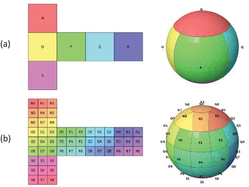
Each cell of the rHEALPix DGGS has a unique identifier (ID). Gibb et al. (2016) define a cell ID to be a string beginning with one of the letters $N,S,O,P,Q,R$ followed by a sequence of zero or more of the integers $0,1,2,\dots ,N_{side}^2-1$. The process of assigning a unique ID to each cell is as follows. First, assign the planar cells at resolution $i=0$ the IDs $N,O,P,Q,R,S$ from top to bottom and left to right. Then, for each resolution $i$ cell with ID $t$ assign its $N_{side}^2$ resolution $i+1$ sub-cells the IDs $t0,t1,\dots ,t\left(N_{side}^2-1\right)$ using a $Z$ space filling curve from top to bottom and left to right (Figure 1). As a result of this approach, the resolution of a cell can easily be determined from its ID by $\left|ID\right|-1$. Note that IDs of planar cells are shared with their corresponding ellipsoidal cells.

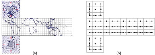
Each planar cell of the rHEALPix DGGS has a nucleus which is defined as its centroid. The nucleus of an ellipsoidal cell is simply the inverse projection of the nucleus of its corresponding planar cell. Given that parallels are projected to horizontal lines in the equatorial region and concentric squares in the polar region (Figure 2(a)), it is clear that planar cell nuclei coincide with projected parallels (Figure 2(b) shows an example of the rHEALPix DGGS with $N_{side}=3$ at resolution $i=1$). Consequently, ellipsoidal cell nuclei must also lie on rings of constant latitude. In the equatorial region, $4N_{side}^{2i}$ ellipsoidal cells lie on $N_{side}^i$ isolatitude rings. In the north polar region, there are $N_{side}^{2i}$ ellipsoidal cells if $N_{side}$ is even, and $N_{side}^{2i}-1$ ellipsoidal cells if $N_{side}$ is odd (excluding the cap cell whose nucleus coincides with the pole), which lie on $⌊N_{side}^i/2⌋$ isolatitude rings. The same can be said of the south polar region. In total, the nuclei of $k=6N_{side}^{2i}$ ellipsoidal cells lie on $2N_{side}^i-1$ (non-pole) isolatitude rings if $N_{side}$ is odd, or $2N_{side}^i$ isolatitude rings if $N_{side}$ is even. Therefore, $k$ cells lie on $O\left(\sqrt{k}\right)$ isolatitude rings (Gibb et al., 2016).

Figure 2. (a) The $\left(0,0\right)$-rHEALPix projection, grid lines represent parallels and meridians (derived from Gibb, 2016). (b) Cell nuclei distributed along the planar projection of parallels.

3. Extending the rHEALPix DGGS

In this section, we introduce a method to determine the isolatitude ring on which the nucleus of a given cell falls using only the cell ID. Importantly, this method is only applicable to the rHEALPix DGGS with $N_{side}=2$ and $N_{side}=3.$ We focus on these two values because (i) the $N_{side}=3$ approach is the smallest integer that produces aligned hierarchies and is the preferred approach in existing work (Bowater & Stefanakis, 2018, 2019b; Gibb, 2016) and (ii) the $N_{side}=2$ approach maximizes the number of resolution levels under a fixed number of cells (i.e. provides a smooth transition) and it can be exactly encoded using 2 bits.

It is important to mention that during our attempts to generalize the method for any $N_{side}$ value, it became clear that a fundamental problem exists with the definition of the rHEALPix DGGS when $N_{side}>3$. This is easily demonstrated by considering the case when $N_{side}=4$. At resolution $i=1$, each base cell with ID $t$ will have 16 sub-cells with IDs $t0,t1,t2,t3,t4,\dots ,t12,t13,t14,t15$. Because six of the cells have IDs consisting of two numerical digits, it is no longer possible to relate cell ID to resolution using the string length of the ID. Note that hexadecimal encoding could potentially solve this problem (when $N_{side}=4$) but such an approach is not considered in the current rHEALPix DGGS definition. More importantly however, cell IDs will no longer be unique across all resolutions. For example, at resolution $i=2$, a cell with ID $t1$ will have 16 sub-cells with IDs $t10,t11,t12,t13,t14,t15,\dots ,t113,t114,t115$ (recall that for each resolution $i$ cell with ID $t$, its $N_{side}^2$ resolution $i+1$ sub-cells have IDs $t0,t1,\dots ,t\left(N_{side}^2-1\right))$. Clearly, there are now cells at resolution $i=1$ and $i=2$ with the same ID. For example, cell ID $t15$ represents a resolution $i=1$ sub-cell of cell $t$, but it is also represents a resolution $i=2$ sub-cell of cell $t1$. This is a major issue because a fundamental requirement for any OGC conformant DGGS is the uniqueness of cell IDs across all resolutions (OGC, 2017b). Therefore, the definition of the rHEALPix DGGS should be amended to account for the issues that arise when $N_{side}>3$, or be constrained to the valid and perhaps most pertinent cases when $N_{side}=2$ and $N_{side}=3$.

In this method, isolatitude rings are expressed as integer values increasing from north to south and ranging from $1\to 2\left(3^i\right)-1$ (excluding the poles) when $N_{side}=3$, and $1\to 2\left(2^i\right)$ when $N_{side}=2$, where $i$ is the resolution of the grid. To ensure this method is compatible with previous work, we utilize the same cell ID notation, indexing method, row notation, and column notation defined in Gibb et al. (2016) and Gibb (2016). In addition, we present a method to convert an isolatitude ring value to its associated geodetic latitude, which ultimately provides a way to calculate the geodetic latitude of a cell’s nucleus via its associated isolatitude ring. We end this section by comparing the computation speed of the proposed methods when $N_{side}=3$ against the method described in Section 6 of Gibb et al. (2016) for calculating the geodetic latitude of a cell’s nucleus for all cell IDs at various resolutions.

To determine the isolatitude ring value associated with a given cell ID, we utilize the planar grid representation of the rHEALPix DGGS rather than the ellipsoidal grid representation because it has the advantage that all cells are squares uniformly positioned in rows and columns at every resolution. That being said, using the planar grid is not without challenges. The main one relates to how lines of constant latitude are represented. In the equatorial region, lines of constant latitude are projected as horizontal lines whereas in the polar region, lines of constant latitude are projected as concentric squares. As a result, this method addresses the equatorial region and polar region separately. Because the conversion process is simplest in the equatorial region, we will start there and then build on this approach for the polar region.

3.1. Equatorial region

First, let us define $M_{NP}^i$ to be the number of non-pole isolatitude rings in the north polar region at resolution $i$, where $M_{NP}^i=\lfloor N_{side}^i/2\rfloor$. Let $M_E^i$ be the number of isolatitude rings in the equatorial region at resolution $i$, where $M_E^i=N_{side}^i$. Also, given the ID of a cell, let the resolution $i$ of that cell be determined by $i=\left|ID\right|-1.$

Now let us consider cells in the equatorial region when $N_{side}=3$ at resolution $i=1$. If we convert the ID of every cell (Figure 3(a)) into row,column notation (as described in Section 4 of Gibb (2016)) and record just the rows (Figure 3(b)), it is clear that every column is identical in this notation. If we take only the digits in row notation to the right of the decimal point, let $r_3$ be the $bas{e}_3$ integer denoted by these digits (Figure 3(c)), and let $r$ be the $bas{e}_{10}$ integer equivalent to $r_3$ (Figure 3(d)), then as we move down the rows from top to bottom, values of $r$ increase from $0\to 2$. For cells at resolution $i=2$, values of $r$ increase from $0\to 8$ as we move down the rows from top to bottom. In general, we observe that for cells at any resolution $i$, values of $r$ increase from $0\to M_E^i-1.$ Knowing this, we can simply offset the values of $r$ by the number of non-pole isolatitude rings in the north polar region $M_{NP}^i$ to determine the isolatitude ring associated with any cell in the equatorial region.

Figure 3. Equatorial region cells at resolution $i=1$ when $N_{side}=3$ expressed using (a) cell IDs, (b) row notation, (c) $r_3$ notation, and (d) $r$ notation.

We can adopt a similar method for cells in the equatorial region when $N_{side}=2.$ However, rather than using $bas{e}_3$ in the construction of row,column notation, we use $bas{e}_2$. For example, at resolution $i=1$ the row notation of cells $P0,P1,P2,P3$, would be $1_3{.0}_2,1_3{.0}_2,1_3{.1}_2,1_3{.1}_2$, respectively. We then let $r_2$ be the $bas{e}_2$ integer denoted by the digits to the right of the decimal point in row notation, and let $r$ be the $bas{e}_{10}$ integer equivalent to $r_2$. Then, as we move down the rows from top to bottom, values of $r$ increase from $0\to M_E^i-1$. Therefore, we can generalize the method for either $N_{side}$ value if we use the relevant $bas{e}_{N_{side}}$ value in the construction of row,column notation and let $r$ be the $bas{e}_{10}$ integer equivalent to $r_{N_{side}}$. Thus, given the ID of an equatorial region cell, we can determine the isolatitude ring on which the nucleus of the cell falls, denoted $I_E$, using $I_E=M_{NP}^i+r+1$.

3.2. Polar region

Let us first consider the case when $N_{side}=3$. In the north polar region at resolution $i=1$, base cell $N$ has nine sub-cells with IDs $N0,N1,N2,\dots ,N8$. Knowing that the north pole is projected to the center of base cell $N$ and thus coincides with the nucleus of cell $N4$, it is clear that the eight remaining cells lie on the only isolatitude ring. In general, at resolution $i$ there are $M_{NP}^i$ non-pole isolatitude rings so it makes sense to assign the value of zero to the cell that covers the north pole. Figure 4 shows this scenario at resolution $i=1$ and $i=2$.

Figure 4. IDs and corresponding isolatitude ring values for (a) resolution $i=1$ cells and (b) resolution $i=2$ cells in cell $N$ when $N_{side}=3$.

At this point, let us define $c_3$ to be the $bas{e}_3$ integer denoted by the digits to the right of the decimal point of the column in row,column notation (as described in Section 4 of Gibb (2016)), and $c$ to be the $bas{e}_{10}$ integer equivalent to $c_3$. Furthermore, let us assign the values $r_0$ and $c_0$ to the cell covering the north pole at resolution $i$, where $r_0=c_0=\lfloor 3^i/2\rfloor =M_{NP}^i$. Then, given the ID of a cell in the north polar region when $N_{side}=3$ at resolution $i$, we can determine the isolatitude ring on which the nucleus of the cell falls, denoted $I_{N_3}$, using $I_{N_3}=max\left(abs\left(r-r_0\right),abs\left(c-c_0\right)\right).$

In the south polar region, the process to determine the isolatitude ring associated with a given cell is similar to the north polar region, with a slight difference. First, let us recall that in total, there are $2N_{side}^i-1$ (non-pole) isolatitude rings if $N_{side}$ is odd. Therefore, if we define $I_{SP}^i$ to be the isolatitude ring value assigned to the cell that covers the south pole at resolution $i$ where $I_{SP}^i=2\left(3^i\right)$, then given the ID of any cell in the south polar region at resolution $i$, we can determine the isolatitude ring on which the nucleus of the cell falls, denoted $I_{S_3}$, using $I_{S_3}=I_{SP}^i-max\left(abs\left(r-r_0\right),abs\left(c-c_0\right)\right).$

With a slight modification, the methods for the north and south polar regions can be extended for the case when $N_{side}=2$. In a similar manner to $r$, let us generalize $c$ by using the relevant $bas{e}_{N_{side}}$ value in the construction of row, column notation and let $c$ be the $bas{e}_{10}$ integer equivalent to $c_{N_{side}}$. Furthermore, if we let $r_0=c_0=\lfloor 2^i/2\rfloor =M_{NP}^i$, then given the ID of a cell in the north polar region when $N_{side}=2$ at resolution $i$, we can determine the isolatitude ring on which the nucleus of the cell falls, denoted $I_{N_2}$, using Equation (1).

(1) $I_{N_2}\left(ID\right)=\left\{\begin{array}{c}max\left(abs\left(r-r_0\right),abs\left(c-c_0\right)\right),r+c<2^i\\ max\left(abs\left(r-r_0\right),abs\left(c-c_0\right)\right)+1,else\end{array}\right.$(1)

For cells in the south polar region, recall there are a total of $2N_{side}^i$ isolatitude rings if $N_{side}$ is even. In addition, there is no sub-cell in base cell $S$ that covers the south pole. Therefore, if we use $2N_{side}^i$ rather than $I_{SP}^i$, then given the ID of a cell in the south polar region when $N_{side}=2$ at resolution $i$, we can determine the isolatitude ring on which the nucleus of the cell falls, denoted $I_{S_2}$, using Equation (2).

(2) $I_{S_2}\left(ID\right)=\left\{\begin{array}{c}2N_{side}^i-max\left(abs\left(r-r_0\right),abs\left(c-c_0\right)\right)+1,r+c<2^i\\ 2N_{side}^i-max\left(abs\left(r-r_0\right),abs\left(c-c_0\right)\right),else\end{array}\right.$(2)

3.3. Isolatitude ring to geodetic latitude conversion

Here we present a method to determine the geodetic latitude associated with an isolatitude ring value $I$ at resolution $i$ when $N_{side}=2$ and $N_{side}=3$.

Let us consider the $\left(0,0\right)$-rHEALPix projection of the unit sphere as a simple rearrangement of the $\left(1,2\right)$-rHEALPix projection presented in Gibb et al. (2016). In this projection, the $\left(x,y\right)$ coordinates of the north pole and south pole are $\left(-3\pi /4,\pi /2\right)$ and $\left(-3\pi /4,-\pi /2\right)$, respectively. In addition, we know from Gibb et al. (2016) that the width of a planar cell $w$ at resolution $i$ is $\left(\pi /2\right)N_{side}^{-i}$. Therefore, if we draw a vertical line between the north pole and south pole coordinates, we can conclude that cell nuclei are evenly spaced at intervals of $w$ along this line.

Now, if we consider the case where $N_{side}=3$, then for a given resolution $i$ there are $2\left(3^i\right)-1$ non-pole isolatitude rings which means there are an equivalent number of cell nuclei on the line between the north pole and south pole. Knowing that cell nuclei coincide with isolatitude rings, we can easily deduce that the first cell nucleus on the line represents the first isolatitude ring $I=1$, the second cell nucleus represents the second isolatitude ring $I=2$, and so on until the last cell nucleus represents isolatitude ring $I=2\left(3^i\right)-1$. Figure 5 shows this scenario at resolution $i=1$. Therefore, given a non-pole isolatitude ring value $I$ and resolution $i$, we can determine the $y$ coordinate of $I$ by $y=\left(\pi /2\right)-wI$ where $w=\left(\pi /2\right)3^{-i}$.

The case where $N_{side}=2$ follows a similar pattern except that for a given resolution $i$ there are $2\left(2^i\right)$ isolatitude rings, and the distance between the first isolatitude ring and the north pole is half the cell width $w$ (similarly for the last isolatitude ring and the south pole). Therefore, we simply need to add an offset to the formula presented above for $N_{side}=3$ to get $y=\left(\pi /2\right)+\left(w/2\right)-wI$ where $w=\left(\pi /2\right)2^{-i}$.

Figure 5. Determining the $y$ coordinate of non-pole isolatitude rings when $N_{side}=3$ at resolution $i=1$.

Lastly, we can use formulae from Appendix A in Gibb et al. (2016) to convert the $y$ coordinate to authalic latitude and then to geodetic latitude. Evidently, by using the methods described above, it is possible to calculate the geodetic latitude of a cell’s nucleus via its associated isolatitude ring by simply converting cell ID to isolatitude ring to geodetic latitude.

3.4. Performance comparison

To verify the simplicity of the proposed methods and to gain a better understanding of their efficiency, we compared the computation speed of the proposed methods for $N_{side}=3$ against the method described in Section 6 of Gibb et al. (2016) for calculating the geodetic latitude of a cell’s nucleus for all cell IDs at various resolutions. Tests were performed using the Python programming language on a 64-bit Windows 10 machine with an Intel Core i7-4800MQ CPU and 8 GB of RAM. Tables 1 and 2 show the average computation speeds in the equatorial region and polar region, respectively.

Table 1. Cell ID to geodetic latitude computation speeds in the equatorial region when $N_{side}=3$.

Resolution	Cells	Proposed method (s)	Gibb et al. (2016) method (s)	Time ratio
3	2916	0.062	0.062	1.00
4	26244	0.512	0.613	1.20
5	236196	4.687	5.675	1.21
6	2125764	42.488	54.138	1.27

Table 2. Cell ID to geodetic latitude computation speeds in the polar region when $N_{side}=3$.

Resolution	Cells	Proposed method (s)	Gibb et al. (2016) method (s)	Time ratio
3	1458	0.034	0.103	3.03
4	13122	0.306	0.897	2.93
5	118098	2.762	8.274	3.00
6	1062882	25.264	76.888	3.04

As shown in Table 2, the average computation speed of the proposed method is approximately three times faster in the polar region. The difference in computation speeds is predominantly because the Gibb et al. (2016) method converts a cell ID to $\left(x,y\right)$ coordinates in the rHEALPix projection followed by a costly matrix-based conversion to $\left(x,y\right)$ coordinates in the HEALPix projection. In contrast, the proposed method converts a cell ID to isolatitude ring and then to a $y$ coordinate in the HEALPix projection using basic arithmetic. As a result, the proposed method avoids the costly conversion, is less computationally complex, and takes less time as a result. Note that both methods use the same formulae to convert the $y$ coordinate in the HEALPix projection to geodetic latitude.

In the equatorial region, both methods have similar computation speeds, as shown in Table 1. Although the proposed method follows the same computational process as for the polar region, the Gibb et al. (2016) method is computationally simpler for the equatorial region. This is evident by noticing that computation speeds in the equatorial region are significantly less than the polar region even though the equatorial region has double the amount of cells at each resolution. The main reason for this is because $\left(x,y\right)$ coordinates are equivalent in both rHEALPix and HEALPix projections which means costly conversions are avoided. In addition, similar to the proposed approach, the $x$ coordinate can be ignored in the computations (unlike in polar region formulae). As a result, both methods have similar complexity and therefore similar speeds.

4. Application of proposed methods for latitudinal data analysis

As mentioned earlier, a DGGS can be thought of as a discrete, multiresolution, digital framework that allows us to store, integrate, analyze, and visualize geospatial big data on a global scale. In this section, we consider latitudinal data analysis and move away from the traditional approach of using the geographic grid, by applying the methods proposed thus far to demonstrate how we can utilize the isolatitude property of the rHEALPix DGGS.

The benefits of analyzing data using a latitudinal approach are clearly emphasized in Kummu and Varis (2011) which to our knowledge, is the most recent and comprehensive paper dedicated to latitudinal data analysis. In this paper, the authors state that although it is common to analyze population, environment, social, and economic development data using administrative boundaries, it can be argued that distance to the equator is one of the key factors affecting the living conditions of human societies. As a result, they use a latitudinal approach based on equal degree latitudinal bands to analyze such data on a global scale to provide an alternative viewpoint that complements administrative boundary-based analyses. In fact, the authors point out that their analyses reveal interesting latitudinal patterns relating to economic development and CO₂ emissions for example, that are not evident in cross-country analyses.

Recall that in the DGGS model, geospatial data (be it vector, raster, or point cloud data) is quantized into cells which can subsequently be retrieved using a cell’s unique ID. In addition, the OGC DGGS Abstract Specification states that a DGGS must include encoding methods to perform algebraic operations on cells and data assigned to them (OGC, 2017b). In fact, this prompted Gibb (2016) to show how cell adjacency and topological relationships (such as contains and touches) can be efficiently computed on the rHEALPix DGGS using cell IDs directly rather than geodetic coordinates. Therefore, once data is embedded into the rHEALPix DGGS, the proposed method of converting a cell ID directly to isolatitude ring without recourse to geodetic coordinates, enables the isolatitude property to be utilized for latitudinal data analysis in such a way that it builds on the work by Gibb (2016) and supports the OGC specification.

To demonstrate the feasibility of the proposed approach, we use the rHEALPix DGGS when $N_{side}=3$ to explore how population changes over Canada in 2015 at different resolutions. The dataset that we use is published by NASA Socioeconomic Data and Applications Center (Center for International Earth Science Information Network-CIESIN-Columbia University, 2018) and includes population estimates (among many other attributes) for administrative units across Canada from 2000 to 2020 (at 5-year intervals). Administrative units are represented as point locations using WGS84 centroid coordinates. In total, the vector dataset includes information for 493193 locations across Canada.

Despite the large volume of points in the dataset, which we found GIS software has difficulty opening, processing the data using the proposed methods is straightforward. First, we need to determine which cell (at a desired resolution) each point location falls in. This can be achieved using formulae described in Gibb et al. (2016) that converts WGS84 geodetic coordinates to cell ID. To accomplish this task, we utilized the coordinate conversion functionality of the open-source web service described in Bowater and Stefanakis (2019b). Second, we must convert the cell ID associated with each point location to isolatitude ring using the proposed methods. This allows us to then aggregate the data based on a simple integer attribute (i.e. isolatitude ring) rather than using costly spatial functions on point geometries. This task was programmed in Python and made use of the pandas Python package because it is fast, flexible, and well suited for performing data analysis on large datasets (see https://pypi.org/project/pandas/).

Figure 6 shows how population changes with isolatitude ring over Canada in 2015 at two different resolutions. Note that a resolution 4 grid ($\sim 114$ km ellipsoidal cell width) corresponds to roughly a $1^{\circ }$ geographic grid ($\sim 111$ km at equator), and a resolution 6 grid ($\sim 13$ km ellipsoidal cell width) corresponds to roughly a $6^{\prime }$ geographic grid ($\sim 11$ km at equator). Both plots show the same general trend of having the majority of the population in the south (corresponding to high isolatitude ring values). This is expected because the bulk of the population live near the US border. Furthermore, on both plots we can identify peaks in the population and the corresponding isolatitude rings at which they occur. The resolution 4 grid provides this information at a small scale ($\sim 114$ km isolatitude ring width), whereas the resolution 6 grid provides a larger scale view ($\sim 13$ km isolatitude ring width). The benefit of the larger scale view is a more fine-grained representation of the change in population which allows us to better identify the main peaks, but also sub-peaks that are lost in the small scale view.

Figure 6. Population change with respect to isolatitude ring at resolution 4 (top) and resolution 6 (bottom).

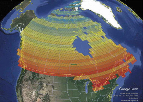
Even though it is clear to see in Figure 6 how the Canadian population changes along the north-south axis, isolatitude ring values by themselves provide no geospatial reference. Therefore, if there is a need to extract geospatial information from the data, for instance the geodetic latitudes associated with population peaks, we could use the simple conversion method proposed in Section 3.3 to convert an isolatitude ring value to geodetic latitude for the peaks of interest. Alternatively, we could convert every isolatitude ring value to geodetic latitude and plot these values against population instead. For example, Figure 7 shows the latitudinal change in the 2015 population at resolution 4 where the two largest peaks can be seen at approximately ${49}^{\circ }$ N and ${44}^{\circ }$ N. To go further, we could take advantage of the inherent nature of a DGGS and visualize the data directly on the earth’s surface using a virtual globe such as ArcGIS Earth or Google Earth. This approach would allow us to rotate the globe and zoom in/out on different areas, thereby providing a more interactive environment in which to explore the data compared to that of a static map visualization. Thus, Figure 8 shows the latitudinal change in the 2015 population at resolution 4 in Google Earth, where isolatitude rings are colored by population ranging from blue (lowest) to red (highest). To create Figure 8, we first utilized the open-source web service from Bowater and Stefanakis (2019b) along with polygon data from Natural Earth (https://www.naturalearthdata.com/) to create a resolution 4 grid over Canada. Then, we used the GeoPandas Python package (http://geopandas.org/) to join the vector grid data with isolatitude ring and population attribute data. Lastly, we used GIS software to color the cells based on population and to create a Keyhole Markup Language (KML) file suitable for Google Earth.

Figure 7. Latitudinal change in population at resolution 4.

Figure 8. A globe-based visualization showing latitudinal change in population at resolution 4 (isolatitude rings are colored by population ranging from blue (lowest) to red (highest)) (©2018 Google).

As we have shown, the isolatitude property of the rHEALPix DGGS can be utilized to facilitate latitudinal data analysis at multiple resolutions. Although we have only considered Canadian population data in our examples, the process could easily be applied to other data sets and at a global scale. Of course, massive global data sets would require more memory and more time to process which may be problematic using current software. However, it is possible to envisage a mature implementation of the rHEALPix DGGS that is capable of efficiently handling data sets of any size and any spatial extent. In such a computing environment, isolatitude ring values could easily be stored as integer attributes for all cell IDs at every resolution. Thus, utilizing the isolatitude property to perform latitudinal data analysis at regional or global scale would be straightforward.

5. Conclusion

Arguably, the most unique property of the rHEALPix DGGS is distribution of $k$ cell nuclei along $O\left(\sqrt{k}\right)$ rings of constant latitude. In this paper, we have explored this isolatitude property. Firstly, we presented a method to determine the isolatitude ring on which the nucleus of a given cell falls. Importantly, the method extends existing work on the rHEALPix DGGS to convert any cell ID to isolatitude ring without recourse to geodetic coordinates. Secondly, we presented a method to convert isolatitude ring to geodetic latitude. Combining these two methods provides a way to determine the geodetic latitude associated with the nucleus of any cell ID. In the polar region especially, this approach shows advantages in terms of computation speed. Lastly, we used the proposed methods to demonstrate how the isolatitude property of the rHEALPix DGGS can be utilized to facilitate latitudinal data analysis at multiple resolutions.

The methods introduced in this paper focus on the rHEALPix DGGS when $N_{side}=3$ and $N_{side}=2$. We focused on these two values because the $N_{side}=3$ approach is the smallest integer that produces aligned hierarchies and is the preferred approach in existing work, while the $N_{side}=2$ approach maximizes the number of resolution levels under a fixed number of cells and can be exactly encoded using 2 bits. Moreover, a fundamental problem exists with the definition of the rHEALPix DGGS when $N_{side}>3$, namely cell IDs are not unique across all resolutions. Therefore, a solution to this issue should be explored in future work.

Finally, the application of the isolatitude property toward harmonic analysis remains to be investigated (Bowater & Stefanakis, 2019a). In their work on the HEALPix DGGS, Gorski et al. (2005) state that the isolatitude property is essential for computational speed in operations involving spherical harmonics, which suggests the rHEALPix DGGS is a good choice for geospatial applications (such as gravitational field modelling) involving harmonic analysis (Gibb et al., 2016). Although the methods presented here could facilitate such work, a thorough investigation on the potential advantages of this approach is yet to be carried out.

Acknowledgments

We would like to thank the anonymous reviewers for their insightful comments that helped to improve the manuscript. This work was funded by the Natural Sciences and Engineering Research Council of Canada (NSERC).

Data availability statement

The data that support the findings of this study are openly available at https://doi.org/10.7927/h4bc3wmt.

Disclosure statement

No potential conflict of interest was reported by the authors.

Additional information

Funding

This work was supported by the Natural Sciences and Engineering Research Council of Canada.

References

- Adams, B. (2017). Wāhi, a discrete global grid gazetteer built using linked open data. International Journal of Digital Earth, 10(5), 490–503.
- Amiri, A., Samavati, F., & Peterson, P. (2015). Categorization and conversions for indexing methods of Discrete Global Grid Systems. ISPRS International Journal of Geo-Information, 4(1), 320–336.
- Amiri, A. M., Bhojani, F., & Samavati, F. (2013). One-to-two digital earth. In G. Bebis et al. (Ed.), Advances in visual computing. ISVC 2013. Lecture notes in computer science (Vol. 8034, pp. 681–692). Berlin, Heidelberg: Springer. doi:10.1007/978-3-642-41939-3_67
- Birk, F. (2018). Design and Implementation of a Scalable Crowdsensing Platform for Geospatial Data ( Master’s Thesis). Ulm University.
- Bowater, D., & Stefanakis, E. (2018). The rHEALPix Discrete Global Grid System: considerations for Canada. Geomatica, 72(1), 27–37.
- Bowater, D., & Stefanakis, E. (2019a, February 22–23). Research directions for the rHEALPix Discrete Global Grid System. Proceedings of the Conference on Spatial Knowledge and Information Canada (SKI 2019), (Vol. 2323). Banff, Alberta, Canada: CEUR-WS.org. [Online]. Retrieved from http://ceur-ws.org/Vol-323/SKI-Canada-2019-7-6-2.pdf.
- Bowater, D., & Stefanakis, E. (2019b). An open-source web service for creating quadrilateral grids based on the rHEALPix Discrete Global Grid System. International Journal of Digital Earth. doi:10.1080/17538947.2019.1645893
- Center for International Earth Science Information Network-CIESIN-Columbia University. (2018). Gridded Population of the World, Version 4 (GPWv4): Administrative Unit Center Points with Population Estimates, Revision 11 [Data set]. Palisades, NY: NASA Socioeconomic Data and Applications Center (SEDAC). doi:10.7927/h4bc3wmt.
- Gibb, R., Raichev, A., & Speth, M. (2016). The rHEALPix Discrete Global Grid System. Retrieved from https://datastore.landcareresearch.co.nz/dataset/rhealpix-discrete-global-grid-system
- Gibb, R. G. (2016). The rHEALPix Discrete Global Grid System. IOP Conference Series: Earth and Environmental Science, 34. doi:10.1088/1755-1315/34/1/012012
- Goodchild, M. F. (2000, March 26–28). Discrete Global Grids for Digital Earth. Proceedings of the 1st International Conference on Discrete Global Grids, Santa Barbara, CA, USA.
- Gorski, K. M., Hivon, E., Banday, A. J., Wandelt, B. D., Hansen, F. K., Reinecke, M., & Bartelman, M. (2005). HEALPix – A framework for high resolution discretization, and fast analysis of data distributed on the sphere. The Astrophysical Journal, 622(2), 759–771.
- Kummu, M., & Varis, O. (2011). The world by latitudes: A global analysis of human population, development level and environment across the north-south axis over the past half century. Applied Geography, 31(2), 495–507.
- Lin, B., Zhou, L., Xu, D., Zhu, A. X., & Lu, G. (2018). A discrete global grid system for earth system modelling. International Journal of Geographical Information Science, 32(4), 711–737.
- Mahdavi-Amiri, A., Alderson, T., & Samavati, F. (2015). A survey of Digital Earth. Computers and Graphics, 53, 95–117.
- OGC (2017a). OGC announces a new standard that improves the way information is referenced to the earth. Retrieved from http://www.opengeospatial.org/pressroom/pressreleases/2656
- OGC (2017b). Topic 21: Discrete Global Grid Systems abstract specification. Retrieved from http://docs.opengeospatial.org/as/15-104r5/15-104r5.html
- Purss, M. B. J., Liang, S., Gibb, R., Samavati, F., Peterson, P., Ben, J., … Saeedi, S. (2017). Applying discrete global grid systems to sensor networks and the Internet of things. IEEE International Geoscience and Remote Sensing Symposium (IGARSS) (pp. 5581–5583). Fort Worth, TX.doi:10.1109/IGARSS.2017.8128269
- Sahr, K., & White, D. (1998). Discrete Global Grid Systems. Proceedings of the 30th Symposium on the Interface, Computing Science and Statistics (pp. 269–278), Minneapolis, Minnesota.
- Sahr, K., White, D., & Kimerling, A. J. (2003). Geodesic Discrete Global Grid Systems. Cartography and Geographic Information Science, 30(2), 121–134.
- Sherlock, M. (2017). Visualisations on a Web-Based View-Aware Digital Earth ( Master’s Thesis). University of Calgary.
- Sirdeshmukh, N. (2018). Utilizing a Discrete Global Grid System For Handling Point Clouds With Varying Locations, Times, and Levels of Detail ( Master’s Thesis). Delft University of Technology.
- Vince, A., & Zheng, X. (2009). Arithmetic and fourier transform for the PYXIS multi-resolution digital earth model. International Journal of Digital Earth, 2(1), 59–79.
- White, D., Kimerling, J. A., & Overton, S. W. (1992). Cartographic and geometric components of a global sampling design for environmental monitoring. Cartography and Geographic Information Systems, 19(1), 5–22.
- Yao, X., & Li, G. (2018). Big spatial vector data management: a review. Big Earth Data, 2(1), 108–129.