A global land cover map produced through integrating multi-source datasets

ABSTRACT

In the past decades, global land cover datasets have been produced but also been criticized for their low accuracies, which have been affecting the applications of these datasets. Producing a new global dataset requires a tremendous amount of efforts; however, it is also possible to improve the accuracy of global land cover mapping by fusing the existing datasets. A decision-fuse method was developed based on fuzzy logic to quantify the consistencies and uncertainties of the existing datasets and then aggregated to provide the most certain estimation. The method was applied to produce a 1-km global land cover map (SYNLCover) by integrating five global land cover datasets and three global datasets of tree cover and croplands. Efforts were carried out to assess the quality: 1) inter-comparison of the datasets revealed that the SYNLCover dataset had higher consistency than these input global land cover datasets, suggesting that the data fusion method reduced the disagreement among the input datasets; 2) quality assessment using the human-interpreted reference dataset reported the highest accuracy in the fused SYNLCover dataset, which had an overall accuracy of 71.1%, in contrast to the overall accuracy between 48.6% and 68.9% for the other global land cover datasets.

KEYWORDS:

• Global land cover
• data integration
• accuracy evaluation

1. Introduction

Land cover represents the understanding of complex interactions between human activities and the environment (Running, 2008). It is an essential variable for land surface, ecological and hydrological modeling (Cramer et al., 1999; DeFries, Townshend, & Hansen, 1999b; Foley et al., 2005; Jung, Henkel, Herold, & Churkina, 2006; Tucker, Townshend, & Goff, 1985), carbon and water cycling (Alcamo, Flörke, & Märker, 2007; Friedlingstein et al., 2006; Ito & Oikawa, 2002; Liu et al., 2011; Oki & Kanae, 2006; Sitch et al., 2008), and climate change studies (Bounoua, DeFries, Collatz, Sellers, & Khan, 2002; Hibbard et al., 2010; Imaoka et al., 2010; Sellers et al., 1997). Global land cover maps have been produced using satellite images (Bartholomé & Belward, 2005; Bicheron et al., 2008; Chen et al., 2015; Friedl et al., 2002; Gong et al., 2013; Hansen, Defries, Townshend, & Sohlberg, 2000; Loveland et al., 2000; Tateishi et al., 2011), and widely used in a variety of applications (DeFries, Field, Fung, Collatz, & Bounoua, 1999a; Giri, 2005; Quaife et al., 2008; Ramankutty, Foley, Norman, & McSweeney, 2002; Verburg, Neumann, & Nol, 2011; You, Wood, & Wood-Sichra, 2009). However, their validation efforts revealed considerable errors and inconsistencies in the land cover maps at the global or continental scales, and further inter-comparison exposed significant disagreements among the maps particularly in the forest and cropland domains (Bai, 2010; DeFries, Hansen, Townshend, Janetos, & Loveland, 2000; Fritz & See, 2008, 2005; Fritz, See, & Rembold, 2010; Giri, 2005; Herold, Mayaux, Woodcock, Baccini, & Schmullius, 2008; Kaptué Tchuenté, Roujean, & De Jong, 2011; Latifovic & Olthof, 2004; Mccallum, Obersteiner, Nilsson, & Shvidenko, 2006; Neumann, Herold, Hartley, & Schmullius, 2007; Quaife et al., 2008; Ran, Li, & Lu, 2010; See & Steffen, 2006; Wu et al., 2008). The errors and disagreements within the maps make it difficult for users to select the proper map for their research, and the uncertainties in the maps will be further transferred and exaggerated to the downstream applications.

However, it is always expensive to improve the quality of the global land cover datasets (Loveland et al., 2000). Another option is to quantify the uncertainty associated with individual land cover dataset and develop a harmonized land cover from these existing datasets. Initiatives like Global Observation of Forest and Land Cover Dynamics (GOFC-GOLD) in conjunction with the Food and Agricultural Organizations (FAO) and the Global Terrestrial Observing Systems (GTOS) have fostered harmonization and strategies for interoperability and synergy of all existing and upcoming global land cover maps (Herold et al., 2006). See and Steffen (2006) present a methodology based on fuzzy logic to generate an improved hybrid land cover map for Northern Europe by taking individual similarities and differences of only two global land cover maps into account. Jung et al. (2006) defined a new land cover classification scheme and used a fuzzy lookup table to integrate existing maps to generate a new global land cover map (SYNMAP). Iwao et al. (2011) created a global land cover map by integrating three land cover maps based on the principle that the majority view prevails, but its accuracy was not significantly higher than that of original maps. Ran et al. (2010) developed a new land cover map using multi-source information based on the Dempster–Shafer evidence theory, but it was limited to China. Schepaschenko et al. (2015) develop a global forest mask through the synergy of remote sensing, crowdsourcing and FAO statistics.

Here we propose a method of fusing multi-source land cover information for land cover datasets. The approach integrates not only land cover datasets but also datasets representing the quantitative attributes of specific land cover types. A new global land cover map was produced by applying the method to fuse existing land cover datasets and global tree-cover and crop-cover datasets. Quality of the new datasets were assessed by examining the consistency among the land cover datasets and the accuracy evaluated using human-interpreted points in China.

2. Data

Eight widely used and publicly available global datasets (Table 1) were selected to produce the fused land cover dataset. These datasets were all produced using coarse resolution (250 m ~ 1 km) satellite imagery, e.g. AVHRR, MODIS, SPOT-4 and MERIS.

Table 1. Global datasets used for producing the fused land cover dataset.

Data set	Sensor	Date	Resolution	Classification approach
GLCC	AVHRR	April 1992-March 1993	1 km	Unsupervised classification with post-classification refinement
UMd	AVHRR	April 1992-March 1993	1 km	Supervised classification decision tree
MODIS LC	MODIS	January 2001-December 2002	500 m	Supervised decision tree, neural networks
GLC2000	SPOT-4	November 1999-December 2000	1 km	Unsupervised classification
GlobCover	MERIS	December 2004-June 2006	300 m	Unsupervised classification
MODIS VCF	MODIS	2000	250 m	Regression tree
MODIS Cropland Probability	MODIS	2000	250 m	Decision tree
AVHRR CFTC	AVHRR	April 1992-March 1993	1 km	Spectral unmixing

2.1. Global land cover maps

The majority (5 out 8) of the selected datasets are land cover maps, describing the distribution of cover types over the global land surface. The datasets and their classifications are described below:

1. Global Land Cover Characterization (GLCC), produced by United States Geological Survey (USGS) to provide land cover in several land cover classification, and GLCC in International Geosphere-Biosphere Programme (IGBP) classification (17 classes) is adopted in the analysis to better matching the other selected land cover datasets (Loveland et al., 1999).

2. University of Maryland land cover product (UMD) is one of the earliest global land cover datasets, which provides land global cover with a simplified version of IGBP classification system, which has 14 classes (Hansen et al., 2000).

3. Moderate Resolution Imaging Spectro-radiometer annual land cover product (MODIS LC) provides global maps of land cover at annual time steps and 500-m spatial resolution for 2001-present (Friedl et al., 2010; Sulla-Menashe & Friedl, 2018). It is one of the standard MODIS data products (Justice et al., 2002), and it supports multiple land cover classification systems, and the dataset with IGBP classification was selected in the analysis.

4. Global Land Cover 2000 (GLC2000) was produced by European Commission’s Joint Research Center (EC-JRC) to provide regional land cover maps for each continent with a flexible classification system based the Land Cover Classification System (LCCS) developed by FAO and UNEP (Di Gregorio & Jansen, 2005). The global map was created by combining those regional land cover maps with converted LCCS code to a less thematically detailed classification LCCS (Bartholomé & Belward, 2005).

5. GLOBCOVER Land Cover Product (GlobCover) is a global land cover dataset produced by European Space Agency (ESA) (Arino et al., 2007; Bicheron et al., 2011). It was produced using the ENVISAT satellite mission’s MERIS (Medium Resolution Image Spectrometer) sensor Level 1B data with a spatial resolution of 300 m. The GlobCover products include a map produced for global land cover in 2005–2006 and another map for 2009. The two maps adopted the FAO LCCS classification system, which has 22 classes, allowing change analysis between the two representing periods.

Efforts have been carried out for validating these global land cover maps. Most of the datasets (i.e. GLCC, UMD, GLC2000 and GlobCover) were validated using sample collected from a designed sampling method and visually interpreted after examining higher resolution corresponding satellite images, i.e. Landsat TM (Thematic Mapper), SPOT (Systeme Probatoire d’Observation dela Tarre), MERIS (Medium Resolution Imaging Spectrometer Instrument) and Google Maps (DeFries, Hansen, Townshend, & Sohlberg, 1998; Friedl et al., 2010; Mayaux et al., 2006; Scepan, Menz, & Hansen, 1999). The MODIS LC dataset was validated based on a cross-validation using subsets of the training data that not been used for the training (Friedl et al., 2010). The reported overall area-weighted accuracies were 66.9% for GLCC (Scepan et al., 1999), 69% for UMD (DeFries et al., 1998), 75% MODIS LC (Friedl et al., 2010), 68.6 ± 5% for GLC2000 (Mayaux et al., 2006) and 67.1% for GlobCover (Mayaux et al., 2006). However, since different approaches and reference databases were used in the evaluation, the reported accuracies are not comparable and should not be considered as truly robust quantitative estimate (Jung et al., 2006).

2.2. Other global datasets

In addition to the land cover datasets, 3 global datasets were selected in the analysis:

1. MODIS Vegetation Continuous Fields (VCF) (MOD44B), which is a collection of annual estimates of several continuous vegetation measurements at 250 m resolution. It provides a global representation of the Earth’s surface as gradations of three components, i.e. tree cover, non-tree vegetation and bare land (Hansen et al., 2003, 2011; Townshend et al., 2011). The percent tree cover estimate is used in the analysis. The MODIS VCF Collection 5 was downloaded from the Global Land Cover Facility (GLCF) at the University of Maryland (http://glcf.umd.edu/data/vcf/).

2. MODIS cropland extent dataset provides estimates of probability of cropland at each 250 m resolution, and it includes two layers, i.e. cropland probability and cropland/non-cropland mask (Pittman, Hansen, Becker-Reshef, Potapov, & Justice, 2010). The MODIS cropland probability layer was derived from a set of multi-year MODIS metrics with incorporating 4 MODIS land bands, NDVI and thermal data, as well as a set of training data like FAO AfriCover and United States National Land Cover Database (NLCD), using classification tree method provided by S-Plus statistical package (Pittman et al., 2010). The probability product was then thresholded to create a discrete cropland/non-cropland indicator map (MODIS Cropland/Non-Cropland), using the data from US Department of Agriculture-Foreign Agricultural Service (USDA-FAS) Production, Supply and Distribution (PSD) database describing per-country acreage of production field crops. MODIS cropland extent probability/mask products over the period 2000–2008 were downloaded from the South Dakota State University (SDSU) (http://globalmonitoring.sdstate.edu/projects/croplands/globalindex.html).

3. AVHRR CFTC (Continuous Fields of Tree Cover) product, which provides estimates of leaf type/leaf longevity for tree classes at 1 km resolution. It was derived from monthly Advanced Very High Resolution Radiometer (AVHRR) NDVI composites over 1992–1993 period using spectral unmixing method (DeFries et al., 2000). The dataset provides fractional estimate of leaf attributes for each pixel, including two layers representing leaf type (broadleaf/needleleaf) and leaf longevity (evergreen/deciduous) separately; while each pair sums up to percentage tree cover. AVHRR CFTC products at 1 km resolution were downloaded from GLCF (http://glcf.umd.edu/data/treecover/).

3. Methodology

The global datasets were released in different formats, structures, spatiotemporal reference systems and semantical classifications. To facilitate data fusion and comparison, these selected global datasets are processed to a uniform geospatial reference system (section 3.1) and translated to comparable semantical variables (section 3.2). Another set of methods are applied to the integration of multi-source datasets (section 3.3), and the evaluation of fused dataset (section 3.4).

3.1. Geographic reference system

MODIS Sinusoidal projection (Seong, Mulcahy, & Usery, 2002) was chosen as the base geographic reference system. The spatial extent is between 180°W ~ 180°E and 55°S ~ 90°N, with a spatial resolution of 1 km. Firstly, the datasets were reprojected to the base spatial reference system with a resolution of 250 m using nearest neighbor resampling. The finer 250 m resolution was selected to reduce precision loss during the re-projecting. The re-projected data are then aggregated to 1 km resolution by selecting the most dominated land cover type within the extent of each 1 km pixel. GeoTIFF format was adopted for storing the output layers.

3.2. Translating semantical definition

3.2.1. Classification scheme

A land cover classification scheme is defined as the target for translating the classes of the input land cover datasets. In order to coordinate the existing land cover types, the target classification scheme was defined upon parameters of classification standard for Plant Functional Types (PFTs) (Diaz & Cabido, 1997; Milchunas & Lauenroth, 1993), i.e. the occurrence of life forms and leaf attributes (leaf type/leaf longevity), which are common classifiers for land cover classification (Neumann et al., 2007). Twelve major classes were defined in the target classification scheme (Table 2), including 8 life forms categories, and 9 classes with leaf type and longevity associated with “Trees”.

Table 2. Target classification scheme defined to adapt major life forms and leaf attributes.

Life form	Leaf type	Leaf longevity	Target classification scheme
Trees	Needleleaf	Evergreen	Evergreen Needleleaf Forest
	Broadleaf	Evergreen	Evergreen Broadleaf Forest
	Needleleaf	Deciduous	Deciduous Needleleaf Forest
	Broadleaf	Deciduous	Deciduous Broadleaf Forest
	Needleleaf	Mixed	Mixed Forest
	Broadleaf	Mixed	Mixed Forest
	Mixed	Evergreen	Mixed Forest
	Mixed	Deciduous	Mixed Forest
	Mixed	Mixed	Mixed Forest
Grassland	–	–	Grassland
Cropland	–	–	Cropland
Shrubland	–	–	Shrubland
Wetland	–	–	Wetland
Water	–	–	Water
Urban and built-up	–	–	Urban and built-up
Others	–	–	Others

3.2.2. Affinity scores

Affinity score measures the fuzzy relationship between a land cover class in the input dataset and its corresponding classes in the target land cover classification scheme. The scores are assigned to the metrics of life form, leaf type and leaf longevity separately. In addition to the land cover datasets, the MODIS VCF and Cropland Probability layers also contribute additional information on trees and cropland classes. The affinity scores for “Trees” and “Cropland” were assigned using different rules individually compared with the other 6 life forms and leaf attributes.

Taking “Tree” as an example, the affinity score for a land cover class in the input datasets is assigned a score between 0 and 100 in terms of the percent canopy cover and sematic definition of the class (see Table 3). For example, assuming C is a class in an input land cover dataset:

1. If the class C matches “Trees” semantically, the score is assigned as the median of canopy cover for C, otherwise the score is assigned 0 if C and “Trees” are independent from each other. For example, the percent tree cover for ‘evergreen needle leaf forest’ in GLCC is >60%, the affinity score of tree cover for this class is set to 80.

2. If the class C is defined as a mosaic type of forest and other vegetation types, and its percent canopy cover is >15%, then the affinity score between C and “Trees” is assigned to the value between the minimum and the median of canopy cover flexibly using expert knowledge, according to forest percent of mosaic class and its semantic relation with “Trees”. Otherwise, if the defined percent canopy cover of C is <10%, then 0 is given to the affinity score between C and “Trees”. For instance, the percent canopy cover for “mosaic: cropland/tree cover/other natural vegetation” in GLC2000 is 15-100%, the affinity score between this class and “Trees” is assigned to 35.

Table 3. Definition example of affinity scores for input class and “Trees”.

Input land cover class	Canopy cover	Affinity score	Life form
Bare ground	0	0	Trees
Grassland	<10%	0	Trees
Tree cover, burnt	>15%	30	Trees
Woodlands	40–60%	50	Trees
Wooded grasslands	10–40%	25	Trees
Evergreen needleleaf forest	>60%	80	Trees

According to the five semantic rules shown in Tables 4 and 5, the affinity score for each input class is assigned a score between 0 and 100 to represent its likelihood to cropland or other classes.

Table 4. Definition example of affinity scores for input classes and “cropland”.

Input land cover class	Semantic rules	Affinity score	Life form
Savannas	Is not	0	Cropland
Mosaic vegetation (grassland/shrubland/forest) (50-70%)/cropland (20-50%)	Has minor parts of	35	Cropland
Cropland/Natural vegetation mosaic	Has parts of	50	Cropland
Mosaic: Cropland/Shrub and/or Herbaceous cover	Has major parts of	50	Cropland
Cultivated and managed areas	Is	100	Cropland

Table 5. Definition example of affinity scores for input classes and target class than are not “Trees” nor “Cropland”.

Input land cover class	Semantic rules	Affinity score	Life form
Barren or sparsely vegetated	Is not	0	Wetland
Woodland	Has minor parts of	25	Grassland
Savannas	Has parts of	50	Grassland
Open shrublands	Has major parts of	75	Shrubland
Urban and built-up	Is	100	Urban and built-up

All affinity scores between the source input class and target class are shown in Appendix 1.

3.3. Data integration

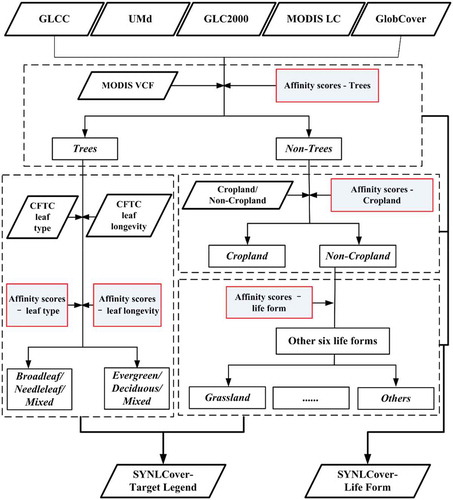
The fused land cover dataset is processed by integrating the input global datasets following four key steps (Figure 1):

1. Fused dataset of Trees and Non-Trees classes are created by combing the tree cover layer from MODIS VCF and tree cover scores produced by applying the affinity scores of “Trees” to the five original global land cover datasets.

2. If a location is identified as high probably of “Trees” at the previous step, the final forest class with leaf type and left longevity in SYNLCover is estimated by combining the MODIS CFTC information.

3. Otherwise, the location is considered as Non-Trees, its likeness of “Cropland” is investigated by combining the MODIS Cropland/Non-Cropland layer and crop scores estimated by applying the affinity scores of “Cropland” to the five global land cover datasets.

4. For location with low likeness of “Cropland”, they are further investigated by examining the affinity scores of the other six life forms calculated from the input global land cover datasets.

Figure 1. Principle of a decision-fuse method used in this study.

Two life form classes including “Trees” and “Cropland” in the fused dataset are determined according to following Equation (1) that calculates the mean score for each life form (Lf) for grid cell with coordinates i and j of SYNLCover:

(1) $S_{Mean}^{Lf}(i,j)=\left(\sum _{M=1}^6{S}_M^{Lf}(i,j)\right)/6$(1)

where:

$S_{Mean}^{Lf}(i,j)$ is the mean score for “Trees” or “Cropland” of SYNLCover;

$S_M^{Lf}(i,j)$ is affinity score for “Trees” or “Cropland” in the pixel (i, j) of the input global dataset M (Appendix 1.1);

M is one of the five input global land cover datasets or MODIS VCF, MODIS Cropland/Non-Cropland;

i and j is current row and column of pixels, respectively.

For the estimation of Trees/Non-Trees, consulting to the threshold for forest classes defined by IGBP, if $S_{Mean}^{Lf}(i,j)$≥ 30, the estimate of life form in pixel (i, j) is “Trees”. Otherwise, if $S_{Mean}^{Lf}(i,j)$< 30, the life form in pixel (i, j) is “Non-Trees”. Similarly, estimation of Cropland/Non-Cropland is made referring to the global threshold that discrete MODIS Cropland Probability into Cropland/Non-Cropland, if $S_{Mean}^{Lf}(i,j)$≥ 43, the estimate of Non-Trees life form in pixel (i, j) is “Cropland”, while if $S_{Mean}^{Lf}(i,j)$< 43, the Non-Trees life form in pixel (i, j) is “Non-Cropland”.

The choice of other six life forms and leaf attributes is made according to Equations (2) and (3), respectively, which calculates total score for other life form (OLf) and leaf attributes (LA) for grid cell with coordinates i and j of SYNLCover:

(2) $S_{Total}^{OLf}\left(i,j\right)=\sum _{M=1}^5{S}_M^{OLf}\left(i,j\right)$(2)

(3) $S_{Total}^{LA}(i,j)=\sum _{N=1}^6{S}_N^{LA}(i,j)$(3)

where:

$S_{Total}^{OLf}(i,j)$ is the total score for life form except “Trees” and “Cropland” (OLf) of SYNLCover;

$S_{Total}^{LA}(i,j)$ is the total score for leaf attributes of “Trees” in SYNLCover;

$S_M^{OLf}(i,j)$is affinity score for OLf in the pixel (i, j) of input global land cover dataset M (Appendix 1.1);

$S_N^{LA}(i,j)$ is affinity score for leaf attributes in the pixel (i, j) of input dataset N (Appendix 1.2);

OLf is each life form of SYNLCover except “Trees” and “Cropland” (Table 2);

LA is leaf attributes including leaf type and leaf longevity of SYNLCover;

M is the five global land cover datasets, N is five input land cover datasets and MODIS CFTC;

i and j is current row and column of pixels, respectively.

The maximum total score of $S_M^{OLf}(i,j)$ and $S_N^{LA}(i,j)$ is chosen as the best estimate of the life form OLf and leaf attributes LA in pixel (i, j) of SYNLCover, respectively. The calculation example for estimate of other life forms is illustrated in Table 6, and the life form class with the highest score wins, here “Grassland”.

Table 6. Calculation example for the best estimate of other life forms.

Dataset	Original land cover class	Life forms
		Grassland	Shrubland	Wetland
GLCC	Open shrubland	50	75	0
UMd	Grassland	100	0	0
GLC2000	Herbaceous cover	100	0	0
MODIS LC	Woody savanna	25	25	0
GlobCover	Mosaic forest or shrubland/grassland	25	75	0
Total score		300	175	0

In case two or more life forms except “Trees” and “Cropland” get the same maximum total score, the decision which life form class wins is made by a random choice. If more than one leaf attributes receive the same maximum score, a decision matrix shown in Table 7 defines the winning leaf attributes. However, if the maximum score for leaf attributes is 0, both leaf type and leaf longevity are set to “Mixed”. This compromise introduces uncertainty, which is fortunately small since this case is very rare and applies only to “Trees” class, so that only part of the leaf attributes of “Trees” is biased.

Table 7. Decision matrix for leaf type (below diagonal) and leaf longevity (above diagonal) in case two leaf classes receive the same maximal score.

Leaf longevity/Leaf type	Mixed	Deciduous/Broadleaf	Evergreen/Needleleaf
Mixed	-	Deciduous	Evergreen
Deciduous/broadleaf	Broadleaf	-	Mixed
Evergreen/needleleaf	Needleleaf	Mixed	-

3.4. Quality assessment

Quality of the fused land cover dataset and the global land cover datasets were assessed using two methods: 1) inter-comparison to evaluate their consistency, and 2) validating the datasets using human-interpreted points in China.

3.4.1. Consistency analysis

The five global land cover datasets are translated to life form and the target class scheme to allow comparison (Appendix 2). The fused SYNLCover is compared to the global land cover datasets by calculating the pixel-based confusion matrices to evaluate its consistency with these global datasets. From the confusion matrices the mean overall consistency is estimated by averaging overall accuracies from comparing datasets to provide a general consistency between SYNLCover and the input datasets:

(4) $Mean{C}_a=(C_{ab}+C_{ac}+{\mathrm{C}}_{ad}+{\mathrm{C}}_{ae}+{\mathrm{C}}_{af})/5$(4)

Where:

C_a* separately denotes the overall consistency between pairs of dataset a and another dataset *;

Indices a-e are SYNLCover, GLCC, UMD, GLC2000, MODIS LC and GlobCover, respectively.

3.4.2. Accuracy assessment

In addition to inter-comparison between these datasets, independently reference dataset is collected by human interpreting land cover types at randomly collected points to provide a comprehensive accuracy evaluation of the fused datasets.

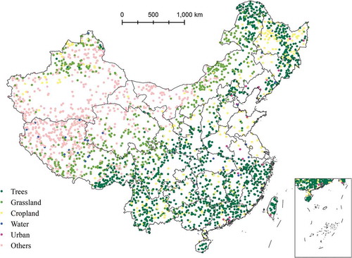
A total of 3000 points were randomly collected in China (Figure 2). Because of the complex of land cover spatial distribution in China, the MODIS land cover dataset was aggregate to six classes (trees, grassland, cropland, water, urban and others) and then used as the stratification for collecting the points to increase the efficiency on representing the various of land covers in China.

Figure 2. Points randomly collected in China through stratified random sampling using the land cover aggregated from MODIS land cover dataset.

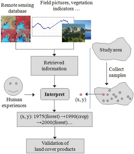
The collected points were visually interpreted by experts in a Web-based tool (Figure 3) (Feng et al., 2012). To help the interpreters on identifying the land cover types, the tool presents maps and charts created from various sources, including: 1) Landsat images from the four epochs (1970s, 1990, 2000 and 2005) provided by the Global Land Survey (GLS) (Gutman et al., 2008; Gutman, Huang, Chander, Noojipady, & Masek, 2013, p. 2) NDVI profile derived from the 8-day composited MODIS Surface Reflectance products (MOD09A1) after cloud and shadow masking; 3) geo-tagged ground photos provided by Google Maps. Eighteen image analysts who have experience in land cover participated in the interpretation task.

Figure 3. Interpreting land cover types at samples collected in a given area (Feng et al., 2012).

Confusion matrix, including overall accuracy (OA), user’s accuracy (UA) and producer’s accuracy (PA), is then calculated between SYNLCover and each of input global land cover datasets using interpreted samples.

4. Results and discussion

4.1. Synlcover fused dataset

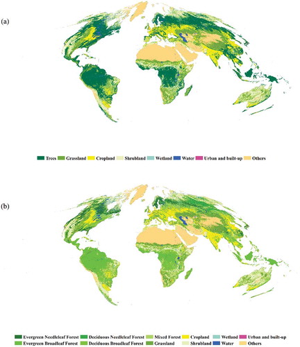
The global SYNLCover life form (Figure 4(a)) and SYNLCover target classification scheme (Figure 4(b)) datasets were produced from the multi-source datasets using the proposed data fused method. They provide distribution of land cover types globally at 1 km resolution. Most of the input datasets presented the global land cover in circa-2000. Although the GLCC and UMD land cover datasets were produced using satellite data in the early 1990s and GlobCover was produced for circa-2005, which are less than a decade away from 2000. Considering their temporal closeness and the insensitivity to temporal changes at the coarse resolution (Fritz et al., 2011), the produced SYNLCover datasets are considered to delineate the global land cover in 2000. Besides the fused global land cover dataset, the affinity scores for each class is outputted, which represent the probability of the class at each pixel. These layers make it possible for applications to explore the mixture of multiple classes within the extent of a pixel extent.

Figure 4. The SYNLCover data sets: (a) SYNLCover-Life Form and (b) SYNLCover-target classification scheme.

4.2. Consistency comparison between the fused dataset and input datasets

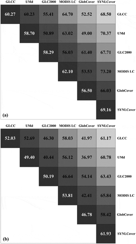
After comparing the SYNLCover and the land cover datasets (Figure 5), the SYNLCover had the highest average overall accuracy for both life form (69.16%) and land cover (61.93%) classes, suggesting improved consistency in the fused dataset over the input land cover datasets. The life form datasets had higher consistency than the land cover datasets, likely due to the higher disagreements among the datasets in the detailed classes introduced in the land cover classes (Jung et al., 2006). Relatively lower consistency was found in MODIS LC, GLCC, UMD and GLC2000. GlobCover get the lowest average overall accuracy for both life forms and land cover dataset.

Figure 5. Overall consistencies between SYNLCover, GLCC, UMd, GLC2000, MODIS LC and GlobCover based on (a) life forms and (b) target classification schemes. Map-specific consistency of each map is given along the diagonal.

4.3. Accuracy validation using interpreted points in china

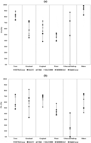
After comparing the fused SYNLCover and the other land cover datasets to the human interpreted dataset in China, it reported an overall accuracy of 71.1% for the SYNLCover-Life Form, which is higher than 68.9% for MODIS LC, 65.2% for GLC20000, and significantly higher than the other three global land cover datasets (57.7% for GlobCover, 57.2% for GLCC and 48.6% for UMD). Also, there were obvious differences across both UA and PA of each life form in the new and the original land cover maps (Figure 6). The UA and PA were between 33.3% and 98.4% for the major land covers except “urban and built-up”, which had lower UA and PA for the three 1-km native resolution (i.e. GLCC, UMD and GLC2000). Preliminary checking suggested that the low accuracy of “urban and built-up” class was mainly due to the poor capacity of delineating the small and fractional urban and built-up by the kilometer resolution coarse spatial scale datasets. Compared with the five original land cover maps, the UA of “Trees”, “Cropland” and “Urban and built-up”, as well as the PA of “Grassland” and “Water” in SYNLCover-Life Form are improved significantly. Figure 6 also presented a general pattern of class accuracy of SYNLCover-Life Form and five input land cover maps. “Trees”, “Grassland”, “Cropland” and “Others” are described with higher accuracy, whereas “Water” and “Urban and built-up” with lower accuracy.

Figure 6. Comparison of (a) user’s and (b) producer’s accuracy of SYNLCover and the five input maps with life forms in China.

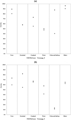
In addition to accuracy comparisons between individual maps, we also compare the accuracy of SYNLCover with the averaged accuracy of five input land cover maps (Figure 7). Result shows that the OA, UA and PA of six life forms of SYNLCover-Life Form, especially for “Trees” and “Grassland”, are higher than the respective average OA, UA and PA of corresponding classes of the five input maps. Obviously, the SYNLCover synthesizes information about the basic appearance of vegetation (forest, shrubland, cropland, herbaceous vegetation), the leaf types (broadleaf and needleleaf), the leaf longevities (evergreen and deciduous), and also other types from the original five land cover maps, VCF, Cropland Probability and CFTC data sets.

Figure 7. Comparison of (a) user’s and (b) producer’s accuracy of life forms in SYNLCover and its corresponding average accuracy of five input maps over China.

5. Conclusions

The existing global land cover datasets provide great value to the land cover user communities, but the low accuracy and inconsistency among the datasets have been affecting the applications of these datasets, especially in land surface process modeling research. We proposed an integration method to produce a global land cover dataset with improved accuracy by synthesizing multi-source global land cover data products using fuzzy logic method. A global 1 km land cover dataset, SYNLCover, was produced using the method with two sets of classification systems to address the need for land cover data regarding delineation of both life forms and land covers. Although these datasets are overlapping between the two classification systems, the life form classes are more generalized than the land cover classes, which further delineated the tree class into forests with different leaf attributes.

The fused SYNLCover was produced by integrating eight global datasets, including five global land cover datasets and three datasets that representing quantitative attributes of specific land cover types. To our knowledge, this effort has been the most comprehensive integration of global land cover datasets. The quality of the fused land cover datasets was evaluated by inter-comparing with the land cover datasets and a reference data produced by human interpretation of 3000 points collected in China. The validation is limited in China, but it was a rigorous assessment of the quality of the datasets because China is considered as one of difficult area for land cover mapping due to its vast geographical extent, highly diverse and fragmental geography (Ran et al., 2010). The validation could also be considered as a representation of the quality of these datasets in larger extent. Both inter-comparison and accuracy assessment suggested that the fused land cover dataset had higher accuracy and consistency than the input global land cover datasets. The life form dataset had higher consistency than the land cover classes, mainly because its classes are more general and the reduced the disagreements between the sub-classes of forests in the land cover classification system. Higher consistencies were found in most of the classes, except in cropland, wetland and urban, which are more difficult to delineate at 1 km resolution. It will likely require land cover mapping at finer spatial scale to be able to capture the fragmentations of these classes. Although eight datasets were used to produce the SYNLCover dataset, more global land cover or related datasets have become available recently (Tuanmu & Jetz, 2014) or will be produced in future, and the presented method could be applied to integrate these datasets to further improve the quality of global land cover datasets.

Data availability statement

The data that support the findings of this study area available from the corresponding author upon request.

Disclosure statement

No potential conflict of interest was reported by the authors.

Additional information

Funding

Funding support for this work were provided by the following programs: the Strategic Priority Research Program of the Chinese Academy of Sciences [Grant No. XDA20100104]; the Basic Resources Investigation of Science and Technology [Grant No.2017FY100900]; and the National Earth System Science Data Sharing Infrastructure, National Science & Technology Infrastructure of China [Grant No.2005DKA32300].

Appendix 1.

Lookup tables of affinity scores

1.1. Affinity scores for life forms

Table

	Trees	Cropland	Grassland	Shrubland	Wetland	Water	Urban	Others
GLCC-IGBP
Evergreen needleleaf forest	80	0	0	0	0	0	0	0
Evergreen broadleaf forest	80	0	0	0	0	0	0	0
Deciduous needleleaf forest	80	0	0	0	0	0	0	0
Deciduous broadleaf forest	80	0	0	0	0	0	0	0
Mixed forest	80	0	0	0	0	0	0	0
Closed shrublands	0	0	0	100	0	0	0	0
Open shrublands	0	0	50	75	0	0	0	0
Woody savannas	45	0	25	25	0	0	0	0
Savannas	20	0	50	50	0	0	0	0
Grasslands	0	0	100	0	0	0	0	0
Permanent wetlands	0	0	0	0	100	0	0	0
Croplands	0	100	0	0	0	0	0	0
Urban and built-up	0	0	0	0	0	0	100	0
Cropland/natural vegetation mosaic	25	50	50	50	0	0	0	0
Snow and ice	0	0	0	0	0	0	0	100
Barren or sparsely vegetated	0	0	25	25	0	0	0	100
Water	0	0	0	0	0	100	0	0
MODIS LC-IGBP
Evergreen needleleaf forest	80	0	0	0	0	0	0	0
Evergreen broadleaf forest	80	0	0	0	0	0	0	0
Deciduous needleleaf forest	80	0	0	0	0	0	0	0
Deciduous broadleaf forest	80	0	0	0	0	0	0	0
Mixed forest	80	0	0	0	0	0	0	0
Closed shrublands	0	0	0	100	0	0	0	0
Open shrublands	0	0	50	75	0	0	0	0
Woody savannas	45	0	25	25	0	0	0	0
Savannas	20	0	50	50	0	0	0	0
Grasslands	0	0	100	0	0	0	0	0
Permanent wetlands	0	0	0	0	100	0	0	0
Croplands	0	100	0	0	0	0	0	0
Urban and built-up	0	0	0	0	0	0	100	0
Cropland/natural vegetation mosaic	25	50	50	50	0	0	0	0
Snow and ice	0	0	0	0	0	0	0	100
Barren or sparsely vegetated	0	0	25	25	0	0	0	100
Water	0	0	0	0	0	100	0	0
UMd-Simplified IGBP
Evergreen needleleaf forest	80	0	0	0	0	0	0	0
Evergreen broadleaf forest	80	0	0	0	0	0	0	0
Deciduous needleleaf forest	80	0	0	0	0	0	0	0
Deciduous broadleaf forest	80	0	0	0	0	0	0	0
Mixed forest	80	0	0	0	0	0	0	0
Woodland	50	0	25	25	0	0	0	0
Wooded grassland	25	0	75	0	0	0	0	0
Closed shrublands	0	0	0	100	0	0	0	0
Open shrublands	0	0	50	75	0	0	0	0
Grassland	0	0	100	0	0	0	0	0
Cropland	0	100	0	0	0	0	0	0
Bare ground	0	0	0	0	0	0	0	100
Urban and built-up	0	0	0	0	0	0	100	0
Water	0	0	0	0	0	100	0	0
GLC2000-FAO LCCS
Tree Cover, broadleaved, evergreen	60	0	0	0	0	0	0	0
Tree Cover, broadleaved, deciduous, closed	70	0	0	0	0	0	0	0
Tree Cover, broadleaved, deciduous, open	30	0	25	25	0	0	0	0
Tree Cover, needleleaved, evergreen	60	0	0	0	0	0	0	0
Tree Cover, needleleaved, deciduous	60	0	0	0	0	0	0	0
Tree Cover, mixed leaf type	60	0	0	0	0	0	0	0
Tree Cover, regularly flooded, fresh water	20	0	0	0	100	0	0	0
Tree Cover, regularly flooded, saline water	20	0	0	0	100	0	0	0
Mosaic: Tree cover/Other natural vegetation	50	0	50	50	0	0	0	0
Tree Cover, burnt(mainly boreal forests)	30	0	0	0	0	0	0	0
Shrub Cover, closed-open, evergreen	0	0	0	100	0	0	0	0
Shrub Cover, closed-open, deciduous	0	0	0	100	0	0	0	0
Herbaceous Cover, closed-open	0	0	100	0	0	0	0	0
Sparse Herbaceous or sparse shrub cover	0	0	50	50	0	0	0	0
Regularly flooded shrub and/or herbaceous cover	0	0	50	50	100	0	0	0
Cultivated and managed areas	0	100	0	0	0	0	0	0
Mosaic: Cropland/Tree Cover/Other Natural Vegetation	35	45	25	25	0	0	0	0
Mosaic: Cropland/Shrub and/or Herbaceous cover	0	45	50	50	0	0	0	0
Bare Areas	0	0	0	0	0	0	0	100
Water Bodies	0	0	0	0	0	100	0	0
Snow and Ice	0	0	0	0	0	0	0	100
Artificial surfaces and associated areas	0	0	0	0	0	0	100	0
GlobCover-FAO LCCS
Post-flooding or irrigated croplands (or aquatic)	0	100	0	0	0	0	0	0
Rainfed croplands	0	100	0	0	0	0	0	0
Mosaic cropland (50-70%)/vegetation (grassland/shrubland/forest) (20-50%)	35	60	50	50	0	0	0	0
Mosaic vegetation (grassland/ shrubland/forest) (50-70%)/cropland (20-50%)	55	40	75	75	0	0	0	0
Closed to open (>15%) broadleaved evergreen or semi-deciduous forest (>5m)	65	0	0	0	0	0	0	0
Closed (>40%) broadleaved deciduous forest (>5m)	70	0	0	0	0	0	0	0
Open (15-40%) broadleaved deciduous forest/woodland (>5m)	30	0	0	0	0	0	0	0
Closed (>40%) needleleaved evergreen forest (>5m)	70	0	0	0	0	0	0	0
Open (15-40%) needleleaved deciduous or evergreen forest (>5m)	35	0	0	0	0	0	0	0
Closed to open (>15%) mixed broadleaved and needleleaved forest (>5m)	65	0	0	0	0	0	0	0
Mosaic forest or shrubland (50-70%)/grassland (20-50%)	55	0	50	75	0	0	0	0
Mosaic grassland (50-70%)/forest or shrubland (20-50%)	35	0	75	50	0	0	0	0
Closed to open (>15%) (broadleaved or needleleaved, evergreen or deciduous) shrubland (<5m)	0	0	0	100	0	0	0	0
Closed to open (>15%) herbaceous vegetation (grassland, savannas or lichens/mosses)	0	0	100	0	0	0	0	0
Sparse (<15%) vegetation	0	0	25	25	0	0	0	0
Closed to open (>15%) broadleaved forest regularly flooded (semi-permanently or temporarily)	20	0	0	0	100	0	0	0
Closed (>40%) broadleaved forest or shrubland permanently flooded – Saline or brackish water	40	0	0	50	100	0	0	0
Closed to open (>15%) grassland or woody vegetation on regularly flooded or waterlogged soil -Fresh, brackish or saline water	25	0	50	50	100	0	0	0
Artificial surfaces and associated areas (Urban areas >50%)	0	0	0	0	0	0	100	0
Bare areas	0	0	0	0	0	0	0	100
Water bodies	0	0	0	0	0	100	0	0
Permanent snow and ice	0	0	0	0	0	0	0	100

1.2. Affinity scores for leaf attributes

Table

	Needleleaf	Broadleaf	Mixed leaf type	Evergreen	Deciduous	Mixed leaf longevity
GLCC-IGBP
Evergreen needleleaf forest	100	0	50	100	0	50
Evergreen broadleaf forest	0	100	50	100	0	50
Deciduous needleleaf forest	100	0	50	0	100	50
Deciduous broadleaf forest	0	100	50	0	100	50
Mixed forest	50	50	100	50	50	100
Closed shrublands	0	0	0	0	0	0
Open shrublands	0	0	0	0	0	0
Woody savannas	0	0	0	0	0	0
Savannas	0	0	0	0	0	0
Grasslands	0	0	0	0	0	0
Permanent wetlands	0	0	0	0	0	0
Croplands	0	0	0	0	0	0
Urban and built-up	0	0	0	0	0	0
Cropland/natural vegetation mosaic	0	0	0	0	0	0
Snow and ice	0	0	0	0	0	0
Barren or sparsely vegetated	0	0	0	0	0	0
Water	0	0	0	0	0	0
MODIS LC-IGBP
Evergreen needleleaf forest	100	0	50	100	0	50
Evergreen broadleaf forest	0	100	50	100	0	50
Deciduous needleleaf forest	100	0	50	0	100	50
Deciduous broadleaf forest	0	100	50	0	100	50
Mixed forest	50	50	100	50	50	100
Closed shrublands	0	0	0	0	0	0
Open shrublands	0	0	0	0	0	0
Woody savannas	0	0	0	0	0	0
Savannas	0	0	0	0	0	0
Grasslands	0	0	0	0	0	0
Permanent wetlands	0	0	0	0	0	0
Croplands	0	0	0	0	0	0
Urban and built-up	0	0	0	0	0	0
Cropland/natural vegetation mosaic	0	0	0	0	0	0
Snow and ice	0	0	0	0	0	0
Barren or sparsely vegetated	0	0	0	0	0	0
Water	0	0	0	0	0	0
UMd-Simplified IGBP
Evergreen needleleaf forest	100	0	50	100	0	50
Evergreen broadleaf forest	0	100	50	100	0	50
Deciduous needleleaf forest	100	0	50	0	100	50
Deciduous broadleaf forest	0	100	50	0	100	50
Mixed forest	50	50	100	50	50	100
Woodland	0	0	0	0	0	0
Wooded grassland	0	0	0	0	0	0
Closed shrublands	0	0	0	0	0	0
Open shrublands	0	0	0	0	0	0
Grassland	0	0	0	0	0	0
Cropland	0	0	0	0	0	0
Bare ground	0	0	0	0	0	0
Urban and built-up	0	0	0	0	0	0
Water	0	0	0	0	0	0
GLC2000-FAO LCCS
Tree Cover, broadleaved, evergreen	0	100	50	100	0	50
Tree Cover, broadleaved, deciduous, closed	0	100	50	0	100	50
Tree Cover, broadleaved, deciduous, open	0	100	50	0	100	50
Tree Cover, needleleaved, evergreen	100	0	50	100	0	50
Tree Cover, needleleaved, deciduous	100	0	50	0	100	50
Tree Cover, mixed leaf type	50	50	100	50	50	100
Tree Cover, regularly flooded, fresh water	0	0	0	0	0	0
Tree Cover, regularly flooded, saline water	0	0	0	0	0	0
Mosaic: Tree cover/Other natural vegetation	0	0	0	0	0	0
Tree Cover, burnt(mainly boreal forests)	0	0	0	0	0	0
Shrub Cover, closed-open, evergreen	0	0	0	50	0	25
Shrub Cover, closed-open, deciduous	0	0	0	0	50	25
Herbaceous Cover, closed-open	0	0	0	0	0	0
Sparse Herbaceous or sparse shrub cover	0	0	0	0	0	0
Regularly flooded shrub and/or herbaceous cover	0	0	0	0	0	0
Cultivated and managed areas	0	0	0	0	0	0
Mosaic: Cropland/Tree Cover/Other Natural Vegetation	0	0	0	0	0	0
Mosaic: Cropland/Shrub and/or Herbaceous cover	0	0	0	0	0	0
Bare Areas	0	0	0	0	0	0
Water Bodies	0	0	0	0	0	0
Snow and Ice	0	0	0	0	0	0
Artificial surfaces and associated areas	0	0	0	0	0	0
GlobCover-FAO LCCS
Post-flooding or irrigated croplands (or aquatic)	0	0	0	0	0	0
Rainfed croplands	0	0	0	0	0	0
Mosaic cropland (50-70%)/vegetation (grassland/shrubland/forest) (20-50%)	0	0	0	0	0	0
Mosaic vegetation (grassland/ shrubland/forest) (50-70%)/cropland (20-50%)	0	0	0	0	0	0
Closed to open (>15%) broadleaved evergreen or semi-deciduous forest (>5m)	0	100	50	100	50	50
Closed (>40%) broadleaved deciduous forest (>5m)	0	100	50	0	100	50
Open (15-40%) broadleaved deciduous forest/woodland (>5m)	0	100	50	0	100	50
Closed (>40%) needleleaved evergreen forest (>5m)	100	0	50	100	0	50
Open (15-40%) needleleaved deciduous or evergreen forest (>5m)	100	0	50	50	50	50
Closed to open (>15%) mixed broadleaved and needleleaved forest (>5m)	50	50	100	50	50	100
Mosaic forest or shrubland (50-70%)/grassland (20-50%)	0	0	0	0	0	0
Mosaic grassland (50-70%)/forest or shrubland (20-50%)	0	0	0	0	0	0
Closed to open (>15%) (broadleaved or needleleaved, evergreen or deciduous) shrubland (<5m)	50	50	50	50	50	50
Closed to open (>15%) herbaceous vegetation (grassland, savannas or lichens/mosses)	0	0	0	0	0	0
Sparse (<15%) vegetation	0	0	0	0	0	0
Closed to open (>15%) broadleaved forest regularly flooded	0	100	50	0	0	0
Closed (>40%) broadleaved forest or shrubland permanently flooded – Saline or brackish water	0	100	50	0	0	0
Closed to open (>15%) grassland or woody vegetation on regularly flooded or waterlogged soil -Fresh, brackish or saline water	0	0	0	0	0	0
Artificial surfaces and associated areas (Urban areas >50%)	0	0	0	0	0	0
Bare areas	0	0	0	0	0	0
Water bodies	0	0	0	0	0	0
Permanent snow and ice	0	0	0	0	0	0
CFTC Leaf Type
Needleleaf (>66%)	100	0	50	0	0	0
Broadleaf (>66%)	0	100	50	0	0	0
Mixed (33-66%)	50	50	100	0	0	0
CFTC Leaf Longevity
Evergreen (>66%)	0	0	0	100	0	50
Deciduous (>66%)	0	0	0	0	100	50
Mixed (33-66%)	0	0	0	50	50	100

Appendix 2.

Conversion table of map classification schemes

Table

Life forms	Target classification schemes	GLCC/MODIS LC	UMd	GLC2000	GlobCover
Trees	Evergreen Needleleaf Forest	Evergreen Needleleaf Forest	Evergreen Needleleaf Forest	Tree Cover, needle-leaved, evergreen	Closed (>40%) needleleaved evergreen forest (>5m)
	Evergreen Broadleaf Forest	Evergreen Broadleaf Forest	Evergreen Broadleaf Forest	Tree Cover, broadleaved, evergreen	Closed to open (>15%) broadleaved evergreen or semi-deciduous forest (>5m)
	Deciduous Needleleaf Forest	Deciduous Needleleaf Forest	Deciduous Needleleaf Forest	Tree Cover, needle-leaved, deciduous	Open (15-40%) needleleaved deciduous or evergreen forest (>5m)
	Deciduous Broadleaf Forest	Deciduous Broadleaf Forest	Deciduous Broadleaf Forest	Tree Cover, broadleaved, deciduous, closed Tree Cover, broadleaved, deciduous, open	Closed (>40%) broadleaved deciduous forest (>5m) Open (15-40%) broadleaved deciduous forest/woodland (>5m)
	Mixed Forest	Mixed Forest Woody Savannas	Mixed Forests Woodland	Tree Cover, mixed leaf type Mosaic: Tree cover/Other natural vegetation Tree Cover, burnt(mainly boreal forests)	Closed to open (>15%) mixed broadleaved and needleleaved forest (>5m)
Grassland	Grassland	Savannas Grasslands	Wooded Grassland Grassland	Herbaceous Cover, closed-open	Mosaic grassland (50-70%)/forest or shrubland (20-50%) Closed to open (>15%) herbaceous vegetation (grassland, savannas or lichens/mosses) Sparse (<15%) vegetation
Cropland	Cropland	Croplands Cropland/Natural Vegetation Mosaic	Cropland	Cultivated and managed areas Mosaic: Cropland/Tree Cover/Other Natural Vegetation Mosaic: Cropland/Shrub and/or Herbaceous cover	Post-flooding or irrigated croplands (or aquatic) Rainfed croplands Mosaic cropland (50-70%)/vegetation (grassland/shrubland/forest) (20-50%) Mosaic vegetation (grassland/shrubland/forest) (50-70%)/cropland (20-50%)
Shrubland	Shrubland	Closed Shrublands Open Shrubland	Closed Shrubland Open Shrubland	Shrub Cover, closed-open, evergreen (with or without sparse tree layer) Shrub Cover, closed-open, deciduous (with or without sparse tree layer)	Mosaic forest or shrubland (50-70%)/grassland (20-50%) Closed to open (>15%) (broadleaved or needleleaved, evergreen or deciduous) shrubland (<5m)
Wetland	Wetland	Permanent Wetlands	–	Tree Cover, regularly flooded, fresh Tree Cover, regularly flooded, saline, (daily variation) Regularly flooded shrub and/or herbaceous cover	Closed to open (>15%) broadleaved forest regularly flooded (semi-permanently or temporarily) – Fresh or brackish water Closed (>40%) broadleaved forest or shrubland permanently flooded – Saline or brackish water Closed to open (>15%) grassland or woody vegetation on regularly flooded or waterlogged soil – Fresh, brackish or saline water
Water	Water	Water Bodies	Water	Water Bodies (natural & artificial)	Water bodies
Urban and built-up	Urban and built-up	Urban and Built-up	Urban and Built-up	Artificial surfaces and associated areas	Artificial surfaces and associated areas (Urban areas >50%)
Others	Others	Snow and Ice Barren or Sparsely Vegetated	Bare ground	Sparse Herbaceous or sparse shrub cover Bare Areas Snow and Ice (natural & artificial)	Bare areas Permanent snow and ice

References

- Alcamo, J., Flörke, M., & Märker, M. (2007). Future long-term changes in global water resources driven by socio-economic and climatic changes. Hydrological Sciences Journal, 52, 247–275.
- Arino, O., Gross, D., Ranera, F., Leroy, M., Bicheron, P., Brockman, C., … Weber, J. L. (2007). GlobCover: ESA service for global land cover from MERIS. International Geoscience and Remote Sensing Symposium (IGARSS) (pp. 2412–2415). doi:10.1109/IGARSS.2007.4423328
- Bai, L., (2010). Comparison and validation of five land cover products over the African continent. Univ. Lund, Sweden, Lund University. Retrieved from https://doi.org/1969905
- Bartholomé, E., & Belward, A. S. (2005). GLC2000: A new approach to global land cover mapping from Earth observation data. International Journal of Remote Sensing, 26, 1959–1977.
- Bicheron, P., Amberg, V., Bourg, L., Petit, D., Huc, M., Miras, B., … Arino, O. (2011). Geolocation assessment of MERIS GlobCover orthorectified products. IEEE Transactions on Geoscience and Remote Sensing, 49, 2972–2982.
- Bicheron, P., Defourny, P., Defourny, P., Brockmann, C., Brockmann, C., Schouten, L., … Arino, O. (2008). GLOBCOVER - Products description and validation report. Levallois-Perret: MEDIAS-France.
- Bounoua, L., DeFries, R., Collatz, G. J., Sellers, P., & Khan, H. (2002). Effects of land cover conversion on surface climate. Climatic Change, 52, 29–64.
- Chen, J., Chen, J., Liao, A., Cao, X., Chen, L., Chen, X., … Mills, J. (2015). Global land cover mapping at 30m resolution: A POK-based operational approach. ISPRS Journal of Photogrammetry and Remote Sensing, 103, 7–27.
- Cramer, W., Kicklighter, D. W., Bondeau, A., Iii, B. M., Churkina, G., Nemry, B., … Schloss, A. L.; Intercomparison, T.P.O.T.P.. (1999). Comparing global models of terrestrial net primary productivity (NPP): Overview and key results. Global Change Biology, 5, 1–15.
- DeFries, R. S., Field, C. B., Fung, I., Collatz, G. J., & Bounoua, L. (1999a). Combining satellite data and biogeochemical models to estimate global effects of human-induced land cover change on carbon emissions and primary productivity. Global Biogeochemical Cycles, 13, 803–815.
- DeFries, R. S., Hansen, M., Townshend, J. R. G., & Sohlberg, R. (1998). Global land cover classifications at 8 km spatial resolution: The use of training data derived from Landsat imagery in decision tree classifiers. International Journal of Remote Sensing, 19, 3141–3168.
- DeFries, R. S., Hansen, M. C., Townshend, J. R. G., Janetos, A. C., & Loveland, T. R. (2000). A new global 1-km dataset of percentage tree cover derived from remote sensing. Global Change Biology, 6, 247–254.
- DeFries, R. S., Townshend, J. R., & Hansen, M. C. (1999b). Continuous fields of vegetation characteristics at the global scale at 1-km resolution. Journal of Geophysical Research, 104, 16911–16923.
- Di Gregorio, A., & Jansen, L. J. M. (2005). Land Cover Classification System (LCCS): Classification Concepts and User Manual. Food and Agriculture Organization of the United Nations. doi:10.1017/CBO9781107415324.004
- Diaz, S., & Cabido, M. (1997). Plant functional types and ecosystem function in relation to global change. Journal of Vegetation Science, 8, 463–474.
- Feng, M., Huang, C., Sexton, J. O., Channan, S., Narasimhan, R., & Townshend, J. R. (2012). An approach for quickly labeling land cover types for multiple epochs at globally selected locations. IEEE International Geoscience and Remote Sensing Symposium, 2012, 6203–6206.
- Foley, J. A., DeFries, R., Asner, G. P., Barford, C., Bonan, G., Carpenter, S. R., … Snyder, P. K. (2005). Global consequences of land use. Science, 80-. doi:10.1126/science.1111772
- Friedl, M. A., McIver, D. K., Hodges, J. C. C. F. F., Zhang, X. Y., Muchoney, D., Strahler, A. H., … Schaaf, C. (2002). Global land cover mapping from MODIS: Algorithms and early results. Remote Sensing of Environment, 83, 287–302.
- Friedl, M. A., Sulla-Menashe, D., Tan, B., Schneider, A., Ramankutty, N., Sibley, A., & Huang, X. (2010). MODIS Collection 5 global land cover: Algorithm refinements and characterization of new datasets. Remote Sensing of Environment, 114, 168–182.
- Friedlingstein, P., Cox, P., Betts, R., Bopp, L., von Bloh, W., Brovkin, V., … Zeng, N. (2006). Climate-carbon cycle feedback analysis: Results from the C 4 MIP model intercomparison. Journal of Climate, 19, 3337–3353.
- Fritz, S., & See, L. (2005). Comparison of land cover maps using fuzzy agreement. International Journal of Geographical Information Science, 19, 787–807.
- Fritz, S., & See, L. (2008). Identifying and quantifying uncertainty and spatial disagreement in the comparison of global land cover for different applications. Global Change Biology, 14, 1057–1075.
- Fritz, S., See, L., McCallum, I., Schill, C., Obersteiner, M., van der Velde, M., … Achard, F. (2011). Highlighting continued uncertainty in global land cover maps for the user community. Environmental Research Letters, 6, 044005.
- Fritz, S., See, L., & Rembold, F. (2010). Comparison of global and regional land cover maps with statistical information for the agricultural domain in Africa. International Journal of Remote Sensing, 31, 2237–2256.
- Giri, C. (2005). Global land cover mapping and characterization: Present situation and future research priorities. Geocarto International, 20, 35–42.
- Gong, P., Wang, J., Yu Le, L. L., Zhao, Y. Y. Y. Y. Y. Y., Zhao, Y. Y. Y. Y. Y. Y., Liang, L., … Chen, J. J. J. (2013). Finer resolution observation and monitoring of global land cover: First mapping results with Landsat TM and ETM+ data. International Journal of Remote Sensing, 34, 2607–2654.
- Gutman, G., Byrnes, R., Masek, J., Covington, S., Justice, C., Franks, S., & Headley, R. (2008). Towards monitoring land-cover and land-use changes at a global scale: The global land survey 2005. Photogrammetric Engineering and Remote Sensing, 74, 6–10.
- Gutman, G., Huang, C., Chander, G., Noojipady, P., & Masek, J. G. (2013). Assessment of the NASA-USGS Global Land Survey (GLS) datasets. Remote Sensing of Environment, 134, 249–265.
- Hansen, M. C., Defries, R. S., Townshend, J. R., & Sohlberg, R. (2000). Global land cover classification at 1 km spatial resolution using a classification tree approach. International Journal of Remote Sensing, 21, 1331–1364.
- Hansen, M. C., DeFries, R. S., Townshend, J. R. G., Carroll, M., Dimiceli, C., & Sohlberg, R. A. (2003). Global percent tree cover at a spatial resolution of 500 meters: First results of the MODIS Vegetation Continuous Fields algorithm. Earth Interact, 7, 1–15.
- Hansen, M. C., Egorov, A., Roy, D. P., Potapov, P., Ju, J., Turubanova, S., … Loveland, T. R. (2011). Continuous fields of land cover for the conterminous United States using Landsat data: First results from the Web-Enabled Landsat Data (WELD) project. Remote Sensing Letters, 2, 279–288.
- Herold, M., Mayaux, P., Woodcock, C. E., Baccini, A., & Schmullius, C. (2008). Some challenges in global land cover mapping: An assessment of agreement and accuracy in existing 1 km datasets. Remote Sensing of Environment, 112, 2538–2556.
- Herold, M., Woodcock, C. E., Di Gregorio, A., Mayaux, P., Belward, A. S., Latham, J., & Schmullius, C. C. (2006). A joint initiative for harmonization and validation of land cover datasets. IEEE Transactions on Geoscience and Remote Sensing, 44, 1719–1727.
- Hibbard, K., Janetos, A., Van Vuuren, D. P., Pongratz, J., Rose, S. K., Betts, R., … Feddema, J. J. (2010). Research priorities in land use and land-cover change for the Earth system and integrated assessment modelling. International Journal of Climatology, 30, 2118–2128.
- Imaoka, K., Kachi, M., Fujii, H., Murakami, H., Hori, M., Ono, A., … Shimoda, H. (2010). Global change observation mission (GCOM) for monitoring carbon, water cycles, and climate change. Proceedings IEEE, 98, 717–734.
- Ito, A., & Oikawa, T. (2002). A simulation model of the carbon cycle in land ecosystems (Sim-CYCLE): A description based on dry-matter production theory and plot-scale validation. Ecological Modelling, 151, 143–176.
- Iwao, K., Nasahara, K. N., Kinoshita, T., Yamagata, Y., Patton, D., & Tsuchida, S. (2011). Creation of new global land cover map with map integration. Journal of Geographical Information Systems, 03, 160–165.
- Jung, M., Henkel, K., Herold, M., & Churkina, G. (2006). Exploiting synergies of global land cover products for carbon cycle modeling. Remote Sensing of Environment, 101, 534–553.
- Justice, C. O., Townshend, J. R., Vermote, E. F., Masuoka, E., Wolfe, R. E., Saleous, N., … Morisette, J. T. (2002). An overview of MODIS land data processing and product status. Remote Sensing of Environment, 83, 3–15.
- Kaptué Tchuenté, A. T., Roujean, J.-L., & De Jong, S. M. (2011). Comparison and relative quality assessment of the GLC2000, GLOBCOVER, MODIS and ECOCLIMAP land cover data sets at the African continental scale. International Journal of Applied Earth Observation and Geoinformation, 13, 207–219.
- Latifovic, R., & Olthof, I. (2004). Accuracy assessment using sub-pixel fractional error matrices of global land cover products derived from satellite data. Remote Sensing of Environment, 90, 153–165.
- Liu, J., Vogelmann, J. E., Zhu, Z., Key, C. H., Sleeter, B. M., Price, D. T., … Jiang, H. (2011). Estimating California ecosystem carbon change using process model and land cover disturbance data: 1951-2000. Ecological Modelling, 222, 2333–2341.
- Loveland, T. R., Reed, B. C., Brown, J. F., Merchant, J. W., Yang, L., Zhu, Z., … Zhu, Z. (2000). Development of a global land cover characteristics database and IGBP DISCover from 1km AVHRR data. International Journal of Remote Sensing, 21, 1303–1330.
- Loveland, T. R., Zhu, Z. L., Ohlen, D. O., Brown, J. F., Reed, B. C., & Yang, L. M. (1999). An analysis of the IGBP global land-cover characterization process. Photogrammetric Engineering and Remote Sensing, 65, 1021–1032.
- Mayaux, P., Eva, H., Gallego, J., Strahler, A. H., Herold, M., Member, S., … Roy, Y. (2006). Validation of the global land cover 2000 map. IEEE Transactions on Geoscience and Remote Sensing, 44, 1728–1739.
- Mccallum, I., Obersteiner, M., Nilsson, S., & Shvidenko, A. (2006). A spatial comparison of four satellite derived 1km global land cover datasets. International Journal of Applied Earth Observation and Geoinformation, 8, 246–255.
- Milchunas, D. G., & Lauenroth, W. K. (1993). Quantitative effects of grazing on vegetation and soils over a global range of environments. Ecological Monographs, 63, 327–366.
- Neumann, K., Herold, M., Hartley, A., & Schmullius, C. (2007). Comparative assessment of CORINE2000 and GLC2000: Spatial analysis of land cover data for Europe. International Journal of Applied Earth Observation and Geoinformation, 9, 425–437.
- Oki, T., & Kanae, S. (2006). Global hydrological cycles and world water resources. Science, 80. doi:10.1126/science.1128845
- Pittman, K., Hansen, M. C., Becker-Reshef, I., Potapov, P. V., & Justice, C. O. (2010). Estimating global cropland extent with multi-year MODIS data. Remote Sensing, 2, 1844–1863.
- Quaife, T., Quegan, S., Disney, M., Lewis, P., Lomas, M., & Woodward, F. I. (2008). Impact of land cover uncertainties on estimates of biospheric carbon fluxes. Global Biogeochemical Cycles, 22. doi:10.1029/2007GB003097
- Ramankutty, N., Foley, J. A., Norman, J., & McSweeney, K. (2002). The global distribution of cultivable lands: Current patterns and sensitivity to possible climate change. Global Ecology and Biogeography, 11, 377–392.
- Ran, Y., Li, X., & Lu, L. (2010). Evaluation of four remote sensing based land cover products over China. International Journal of Remote Sensing, 31, 391–401.
- Running, S. W. (2008). Climate change: Ecosystem disturbance, carbon, and climate. Science, 80. doi:10.1126/science.1159607
- Scepan, J., Menz, G., & Hansen, M. C. (1999). The DlsGover validation lnterpretation lmage process. Photogrammetric Engineering and Remote Sensing, 65, 1075–1081.
- Schepaschenko, D., See, L., Lesiv, M., McCallum, I., Fritz, S., Salk, C., … Ontikov, P. (2015). Development of a global hybrid forest mask through the synergy of remote sensing, crowdsourcing and FAO statistics. Remote Sensing of Environment, 162, 208–220.
- See, L. M., & Steffen, F. (2006). A method to compare and improve land cover datasets: Application to the GLC-2000 and MODIS land cover products. IEEE Transactions on Geoscience and Remote Sensing, 44, 1740–1746.
- Sellers, P. J., Dickinson, R. E., Randall, D. A., Betts, A. K., Hall, F. G., Berry, J. A., … Henderson-Sellers, A. (1997). Modeling the exchanges of energy, water, and carbon between continents and the atmosphere. Science, 275(80), 502–509.
- Seong, J. C., Mulcahy, K. A., & Usery, E. L. (2002). The sinusoidal projection: A new importance in relation to global image data. The Professional Geographer, 54, 218–225.
- Sitch, S., Huntingford, C., Gedney, N., Levy, P. E., Lomas, M., Piao, S. L., … Woodward, F. I. (2008). Evaluation of the terrestrial carbon cycle, future plant geography and climate-carbon cycle feedbacks using five Dynamic Global Vegetation Models (DGVMs). Global Change Biology, 14, 2015–2039.
- Sulla-Menashe, D., & Friedl, M. A. (2018). User guide to collection 6 MODIS land cover (MCD12Q1 and MCD12C1) Product 1–18. doi:10.5067/MODIS/MCD12Q1
- Tateishi, R., Uriyangqai, B., Al-Bilbisi, H., Ghar, M. A., Tsend-Ayush, J., Kobayashi, T., … Sato, H. P. (2011). Production of global land cover data – GLCNMO. International Journal of Digital Earth, 4, 22–49.
- Townshend, J. R., Hansen, M. C., Carroll, M., DiMiceli, C., Sohlberg, R., & Huang, C. (2011). Vegetation continuous fields MOD44B, 2010 percent tree cover [WWW document]. Collect, 5. Univ. Maryland, Coll. Park. Maryl. Retrieved from http://glcf.umiacs.umd.edu/data/vcf/
- Tuanmu, M. N., & Jetz, W. (2014). A global 1-km consensus land-cover product for biodiversity and ecosystem modelling. Global Ecology and Biogeography. doi:10.1111/geb.12182
- Tucker, C. J., Townshend, J. R. G., & Goff, T. E. (1985). African land-cover classification using satellite data. Science, 80-. 227, 369–375.
- Verburg, P. H., Neumann, K., & Nol, L. (2011). Challenges in using land use and land cover data for global change studies. Global Change Biology. doi:10.1111/j.1365-2486.2010.02307.x
- Wu, W., Shibasaki, R., Yang, P., Ongaro, L., Zhou, Q., & Tang, H. (2008). Validation and comparison of 1 km global land cover products in China. International Journal of Remote Sensing, 29, 3769–3785.
- You, L., Wood, S., & Wood-Sichra, U. (2009). Generating plausible crop distribution maps for Sub-Saharan Africa using a spatially disaggregated data fusion and optimization approach. Agricultural Systems, 99, 126–140.