Linking observation, modelling and satellite-based estimation of global land evapotranspiration

ABSTRACT

Evapotranspiration (ET) is a pivotal process for ecosystem water budgets and accounts for a substantial portion of the global energy balance. In this paper, the exited actual ET main datasets in global scale, and the global ET modeling and estimates were focused on discussion. The Source energy balance (SEB) models, empirical models and other process-based models are summarized. Accuracy for ET estimates by SEB models highly depends on accurate surface temperature retrieval, and SEB models are hard to apply in large heterogeneous surface. The Penman–Monteith (PM) equations are thought to be with considerable sound mechanism. However, it involves large number of parameters, which are not all global available. A simplified PM equation by Priestley and Taylor (PT) is found to perform well on well-watered surface. For both PM and PT equations in estimating ET, the key is to consider the constraint from surface resistance primarily water stress. Empirical models are simple but the accuracy of which highly depends on training samples. Coupling satellite data into ET models can improve ET estimates with higher resolution spatiotemporal information inputs; However, finding the most proper way to estimate global ET remains problematic. Several reasons for this issue are also analyzed in this review.

KEYWORDS:

• Evapotranspiration
• FLUXNET
• remote sensing
• estimation model
• global scale

1. Introduction

Terrestrial evapotranspiration (ET), defined as the return of water vapour to the atmosphere by evaporation from land and water surfaces and by the transpiration of vegetation, is an important biophysical process and a critical component of land-atmosphere hydrological cycle (Badgley, Fisher, Jiménez, Tu, & Vinukollu, 2015; Bai et al., 2017; Fisher et al., 2017; Fisher, Tu, & Baldocchi, 2008; Fisher, Whittaker, & Malhi, 2011; Yan et al., 2012; Zhang, Fu, & Wang, 2000) (Figure 1).

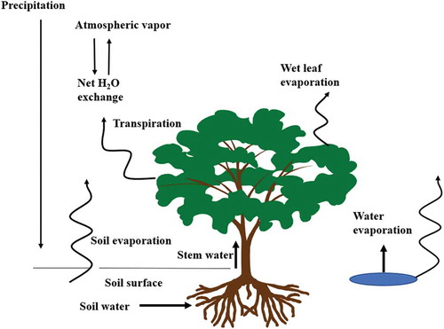
Generally, over the land, the evaporation (E) process includes water evaporating from water body, wet soil and wet vegetation layer above the soil surface, while transpiration (T) is a process of water up-taking via the leaf stoma coupled with carbon emission during photosynthesis process (Bai, Zhang, Zhang, Yao, & Magliulo, 2018; Fisher et al., 2011; Wang & Dickinson, 2012), and is the dominating water fluxes (Jasechko et al., 2013) (Figure 2). Evapotranspiration (ET) is a biophysical process surface energy cycle involved (Yan et al., 2012, 2013), it accounts for about half of the land surface energy consuming and returning about 60% of the land precipitation into the atmosphere on global scale (Jung et al., 2010), which help cooling the land surface. The energy living land surface with vapor is called the latent heat $\lambda E$. So the process of ET has great impact on global climate and meteorology (Fisher et al., 2017; Mu, Zhao, & Running, 2011), and to obtain accurate global ET in long terms can help us in understanding climate change and the water cycle (Fisher et al., 2011; Yan et al., 2013). This issue still remains problematic (Chen et al., 2014; Fisher et al., 2011), even though many methods have been proposed.

Figure 1. Evapotranspiration includes plant transpiration, canopy interception evaporation, and soil evaporation (downloaded from https://science.nasa.gov/earth-science/oceanography/ocean-earth-system/ocean-water-cycle/).

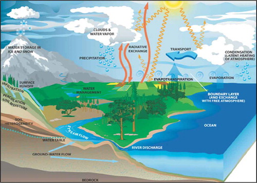
Figure 2. Land evapotranspiration consists of transpiration from vegetation and evaporation from water day, wet leaf, and soil.

The components of ET may affect long-term plant evolution and groundwater stores (Miralles, De Jeu, Gash, Holmes, & Dolman, 2011). Accounting for the ET components across different biomes is essential for the evaluation of the impacts of carbon dioxide enrichment and land-use changes (Fisher et al., 2017; Schlesinger & Jasechko, 2014). Even drought assessment requires considering not only precipitation but also the other meteorological parameters such as an ET, so ET generally acts as an indicator of drought severity over regional or global scale (Shao, Yao, Zhang, & Li, 2013). Thus, observation and estimated methods of global land ET are necessary for more accurately understand the distribution and dynamic in spatiotemporal scales. For agriculturalists, accurate estimates of ET can provide knowledge of how much irrigation may be required (Fisher et al., 2011).

A large variety of evapotranspiration (ET) models and measurements have been reported in the literature (Ershadi, McCabe, Evans, Chaney, & Wood, 2014; Fisher et al., 2011; McCabe, Miralles, Holmes, & Fisher, 2019; Mueller et al., 2013; Stoy et al., 2019; Wang & Dickinson, 2012). However, ET estimation over extended areas including different biomes and climate zones is still subject to significant uncertainties (Fisher et al., 2017; Hssaine et al., 2018; Mueller et al., 2011 &, 2013). One of the main reasons is that in modeling ET lies in a lack of relevant input data available at the desired space and time scales (Bai et al., 2018, 2017; Fisher et al., 2011; Hssaine et al., 2018; Pereira, Allen, Smith, & Raes, 2015). The sensitivity of the model to different input parameters may change with spatial scale (Fisher et al., 2011, 2017). The accuracy of ET estimates at a given scale thus currently represents a trade-off between model complexity and realism, which is usually related to the number of model parameters and forcing variables, and the availability of data that generally decreases at the spatial extent (Allen, Pereira, Howell, & Jensen, 2011; Gharsallah, Facchi, & Gandolf, 2013; Hssaine et al., 2018). In recently, the satellite remote sensors provide very relevant information to feed ET models such as vegetation indices (VI), leaf area index (LAI), land-surface temperature (T_s), relative humidity (RH), and soil moisture (SM), etc. (Bai et al., 2018; Fisher et al., 2008; 2011; Polhamus, Fisher, & Tu, 2013; Purdy et al., 2018; Yan et al., 2012), so as to provide a channel for developing the satellite-based estimation model of global land ET.

The objective of this paper is to review the observation, modelling and satellite-based estimation of global terrestrial ET. To address this issue, firstly, we discuss the exited global actual evapotranspiration main datasets which widely used for the climate research recently, then the overview of global ET models derived from satellite is presented, and our new developed model focusing on ET estimation in Mediterranean climate region considering vertical root distribution, and satellite-retrieved vegetation information, and a new comprehensive model coupled temporal dynamics of optimum stomatal conductance with ET model were also presented for modeling of daily ET of C₃ and C₄ crops. In the last, the global ET estimates and its dynamics, and uncertainty were given.

2. Exited main global actual evapotranspiration (AET) datasets

2.1. Field observation of AET

Field observation of global ET or $\lambda E$ and its distribution is still suspense, but some down-scale methods have been proposed. These methods have been reviewed (Fisher et al., 2011; Wang & Dickinson, 2012). Generally, Eddy covariance (EC), Pan evaporation, Sap flow, Bowen ratio, Lysimeter, Large-aperture scintillometers (LAS), surface water balance, and atmospheric water balance were used to measure or calculate ET in field and landscape scales (French, Hunsaker, & Thorp, 2015; Gebler et al., 2015; Pastorello et al., 2017; Valayamkunnath, Sridhara, Zhao, & Allen, 2018). Among othem, the EC method is widely used.

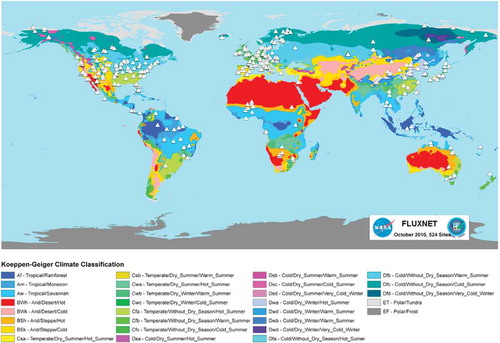
FLUXNET is a global network of micrometeorological tower sites that use EC methods to measure the exchanges of carbon dioxide, water vapor, and energy between terrestrial ecosystems and the atmosphere. More than 500 tower sites around the world are operating on a long-term basis (https://daac.ornl.gov/). The global FLUXT network is working with EC systems (Wang & Dickinson, 2012) (Figure 3), which has 683 sites all over the world by 2014 (Center, 2013).

Figure 3. A map of FLUXNET sites and climate (Koppen-Geiger classification) (Figure is adopted from Wang & Dickinson (2012), i.e. downloaded from http://www.fluxnet.ornl.gov/fluxnet/graphics.cfm).

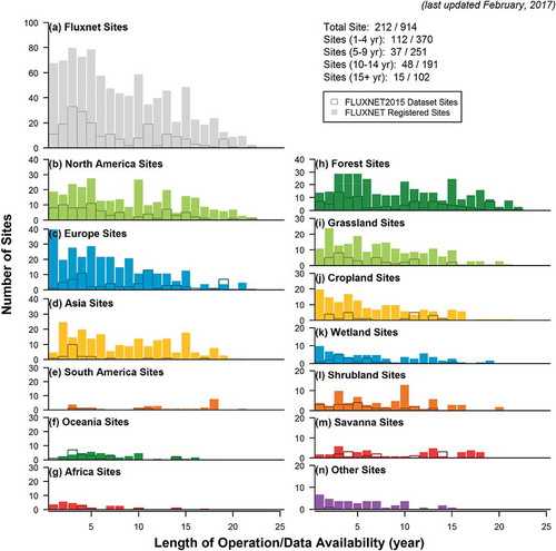
Figure 4 summarizes the tower sites registered in FLUXNET (closed bars) and included in the FLUXNET2015 Dataset (open bars). “Registered sites” represent sites that have been registered in fluxdata.org, FLUXNET-ORNL, AmeriFlux, ICOS, AsiaFlux, OzFlux, or ChinaFlux. Sites are grouped by regions (b-g) and vegetation classification (h-n) (IGBP: International Geosphere–Biosphere Programme). Forest: ENF+DBF+EBF+MF, Grassland: GRA, Cropland: CRO+CVM, Wetland: WET, Shrubland: OSH+CSH, Savanna: SAV+WSA, Other: BSV+URB+WAT+SNO (last updated in February 2017) (https://fluxnet.fluxdata.org/sites/site-summary/).

Figure 4. Summary of tower sites that are registered in FLUXNET (closed bars) and included in the FLUXNET2015 Dataset (open bars). “Registered sites” represent sites that have been registered in fluxdata.org, FLUXNET-ORNL, AmeriFlux, ICOS, AsiaFlux, OzFlux, or ChinaFlux. Sites are grouped by regions (b-g) and vegetation classification (h-n) (IGBP: International Geosphere–Biosphere Programme). Forest: ENF+DBF+EBF+MF, Grassland: GRA, Cropland: CRO+CVM, Wetland: WET, Shrubland: OSH+CSH, Savanna: SAV+WSA, Other: BSV+URB+WAT+SNO (last updated in February 2017) (figure downloaded from https://fluxnet.fluxdata.org/sites/site-summary/).

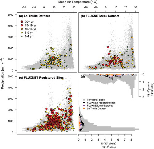
Figure 5 presents the distribution of FLUXNET sites across temperature and precipitation ranges (under Whittaker’s biome classification), compared to land surface from the terrestrial globe. The length of the record of sites is represented in the circle sizes and colors (a-c). Panel (a) shows the sites included in the La Thuile 2007 Dataset; panel (b) shows the sites included in the FLUXNET2015 Dataset; panel (c) shows all sites present in FLUXNET; and, panel (d) compares the distribution of land surface, FLUXNET sites, and sites in the FLUXNET2015 Dataset across these temperature-precipitation ranges (Pastorello et al., 2017, EOS). (https://fluxnet.fluxdata.org/about/)

Figure 5. Distribution of FLUXNET sites across temperature and precipitation ranges (a.k.a., Whittaker’s biome classification), compared to land surface from the terrestrial globe. The length of the record of sites is represented in the circle sizes and colors (a-c). Panel (a) shows the sites included in the La Thuile 2007 Dataset; panel (b) shows the sites included in the FLUXNET2015 Dataset; panel (c) shows all sites present in FLUXNET; and, panel (d) compares the distribution of land surface, FLUXNET sites, and sites in the FLUXNET2015 Dataset across these temperature-precipitation ranges. (Pastorello et al., 2017, EOS) (Figure downloaded from https://fluxnet.fluxdata.org/about/).

The EC system measures wind speed in both vertical and horizontal directions, the carbon dioxide concentration, latent heat flux ($\lambda E$), sensible heat flux ($H$), precipitation, speed of sound used to derive air temperature ($T_a$) (Wang & Dickinson, 2012; Yan et al., 2012). The observation precision for $\lambda E$ of the flux site is relatively high about 5–20% (Foken, 2008; Wang & Dickinson, 2012). However, it has long been known that the EC method has the problem of energy unbalance and enclosure (Jiang & Islam, 2001; Masseroni, Corbari, & Mancini, 2014; Wang & Liang, 2008), i.e., the measured energy flux components $\lambda E$, $H$ and $G$ (ground heat flux) do not meet the energy balance equation (see Equation (1)(1) $\lambda E=R_n-H-G$(1) ).

(1) $\lambda E=R_n-H-G$(1)

where $R_n$ is the surface net radiation. This energy balance equation is the basis for many $\lambda E$ retrieval models. Methods are proposed for addressing this problem (Masseroni et al., 2014; Twine et al., 2000). A simple correction of $\lambda E$ ($\lambda E_C$) (see Equation (2)(2) $\lambda E_C=\frac{\lambda E}{R_C}$(2) ) was proposed by Twine et al. (2000) and applied in Yao et al. (2015), where $R_c$ is the ration for the sum of original $\lambda E$ and $H$ to $R_n-G$.

(2) $\lambda E_C=\frac{\lambda E}{R_C}$(2)

From a global view, a flux site is just a point measuring a limited region within several hundred meters (Yao et al., 2015), these sites cannot represent for the global land (Wang, Dickinson, Wild, & Liang, 2010a).

The data of flux sites are used to validate satellite-based retrieval models, which could be used to retrieval the distribution of $\lambda E$ on regional, continental and global scales (Fisher et al., 2017, 2008; Hao, Zhang, & Yao, 2015; Jin, Randerson, & Goulden, 2011; Mu et al., 2011; Nagler et al., 2005; Yan et al., 2012; Yao et al., 2017).

2.2. MTE AET dataset

The MTE (the model tree ensemble) AET data are an upscaled FLUXNET dataset with a monthly timescale and in 0.5° spatial resolution from 1982 to 2011 (Jung, Reichstein, & Bondeau, 2009; Jung et al., 2010, 2011). The MTE datasets are a machine-learning approach to establish a statistical relationship (linear regression) between the EC observations (the La Thuile dataset) and 29 explanatory variables (including fraction of absorbed photosynthetically active radiation (fAPAR), temperature, precipitation, potential radiation, global land cover datasets (SYNMAP)). This approach is data-driven and largely independent of theoretical model assumptions. Hence, as a proxy for the FLUXNET observations, the MTE datasets have been widely used as a reference in global carbon and water cycle studies.

2.3. BESS AET dataset

The Breathing Earth System Simulator (BESS) is a simplified process-based model that couples atmosphere and canopy radiative transfers, canopy photosynthesis, transpiration, and energy balance (Jiang & Ryu, 2016; Ryu et al., 2011). In the model, BESS AET is estimated based on the quadratic Penman–Monteith equation. The input datasets of the BESS model are MODIS (Moderate Resolution Imaging Spectroradiometer) atmosphere and land products (including MCD12Q1, MOD04 aerosol, MOD06 cloud, MOD07 atmosphere profile, MOD11A1 land-surface temperature (T_s), MOD15A2 LAI (Leaf Area Index), and MCD43B3 albedo), wind speed data from the National Center for Environmental Prediction/National Center for Atmospheric Research (NCEP/NCAR) reanalysis datasets, global clumping index map derived from MODIS BRDF (Bidirectional reflectance distribution function) product, global forest canopy height product from the Geoscience Laser Altimeter System (GLAS) aboard ICESat (Ice, Cloud, and land Elevation Satellite), and global C₃ and C₄ distribution map. The BESS AET data with monthly scale in 1–5 km resolution and 0.5° resolution are available at http://environment.snu.ac.kr/.

2.4. MODIS AET dataset

The MODIS retrieved AET algorithm is based on the Penman–Monteith equation to estimate global AET (Cleugh, Leuning, Mu, & Running, 2007; Mu, Heinsch, Zhao, & Running, 2007), which has been further improved by Mu et al. (2011). In the improved algorithm, MODIS AET is calculated as the sum of the daytime and nighttime evapotranspiration. The improved algorithm also simplifies the calculation of vegetation cover fraction and improves the estimation of stomatal conductance (g_st), aerodynamic resistance ($r_0$), and boundary layer resistance ($r_{bl}$). Moreover, the improved algorithm separates the dry canopy surface from the wet and divides the soil surface into a saturated wet surface and a moist surface (Mu et al., 2011). The datasets used in the MODIS AET algorithm include daily meteorological data from the Global Modeling and Assimilation Office (GMAO-MERRA), MOD12Q1. Here, we used annual MODIS AET (MOD16A3) with 1-km spatial resolution for mapping AET. The MODIS AET data are downloaded from the Numerical Terra dynamic Simulation Group (NTSG) of the University of Montana (http://files.ntsg.umt.edu/data/NTSG _Products/).

2.5. ECOSTRESS ET product

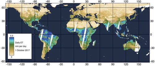
The ECOsystem Spaceborne Thermal Radiometer Experiment on Space Station (ECOSTRESS) was launched on June 29, 2018. The ECOSTRESS mission measures the temperature of plants to better understand how much water plants need and how they respond to stress (Fisher, 2015, 2018; Fisher et al., 2020). ECOSTRESS is attached to the International Space Station (ISS) and collects data over the conterminous United States (CONUS) as well as key biomes and agricultural zones around the world and selected FLUXNET (http://fluxnet.fluxdata.org/about/) validation sites. A map of the acquisition coverage can be found on the ECOSTRESS website (https://ecostress.jpl.nasa.gov/science). The ECOSTRESS standard products will include evapotranspiration (i.e., PT-JPL, described in Section 3.2.4) as well as evaporative stress index and water use efficiency (Fisher, 2015, 2018; Fisher et al., 2020). These products can be used to assess vegetation water stress over managed (such as agricultural) and natural landscapes and have the potential to support management decisions. The ECO3ETPTJPL Version 1 is a Level 3 (L3) product that provides ET generated from data acquired by the ECOSTRESS radiometer instrument according to the Priestly-Taylor Jet Propulsion Laboratory (PT-JPL) algorithm described in the Algorithm Theoretical Basis Document (ATBD) (Fisher, 2015, Figure 6). The ECO3ETPTJPL Version 1 data product contains layers of instantaneous ET, daily ET, canopy transpiration, soil evaporation, ET uncertainty, and interception evaporation (Fisher, 2018).

Figure 6. Global evapotranspiration (mm d⁻²) for a single day at 1 km resolution for PT-JPL from MODIS (Fisher, 2018).

2.6. The spatial distribution of AET over the globe

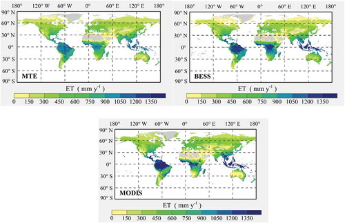
Figure 7 shows the spatial distribution of AET over the globe, the evergreen broadleaf forest areas in tropical region have the highest mean annual AET values, exceeding to 1200 mmyr⁻¹. Additionally, the southeast of all continents between latitudes 25° and 40°, such as southeastern China, southeastern United States, southeastern Brazil, southeastern Africa, and southeastern Australia where corresponding to humid subtropical climate, also have the relatively high AET values. Low mean annual AET values (<150 mmyr⁻¹) are observed in high latitudes and arid regions in the center of Eurasia and the southwest of all continents between latitudes 20° and 40°.

Figure 7. The spatial patterns of the mean annual AET with MTE observation, BESS and MODIS estimates over 2001–2011.

3. Global Evapotranspiration (ET) models

Retrieval models for ET (i.e., $\lambda E)$ established on global scale are all based on basic evapotranspiration theories, which have been reviewed (Fisher, Whittaker, & Malhi, 2011; McCabe et al., 2019; Ren, Yang, Li, & Zhang, 2013; Stoy et al., 2019; Wang & Dickinson, 2012). Models in different spatial scale for ET or $\lambda E$ include Penman-Montieth model (Allen, Pereira, Raes, & Smith, 1998; Penman, 1956), its simplified form Priestley–Taylor model (1972), and modified Priestley–Taylor (PT-JPL) (Fisher et al., 2008, 2011); energy balance models based on Equation (1)(1) $\lambda E=R_n-H-G$(1) , which include one source layer models (SEB), e.g., SEBAL (Bastiaanssen, Menentia, Feddesb, & Holtslagc, 1998a, 1998b), two source layers models (TSEB) (Colaizzi et al., 2012) and multi-source layers models (Merlin et al., 2014); empirical models (Jung et al., 2009, 2010), and integrated models (Bai et al., 2017, 2018). Some research efforts have been made for the ET comparisons and validations (Ershadi et al., 2014; McCabe et al., 2016, 2019; Michel et al., 2016; Miralles et al., 2016; Vinukollu, Wood, Ferguson, & Fisher, 2011). This review is going to keep an eye on the advanced development of these models in ET estimation on global scale, analyze their advantage and disadvantage and give suggestions for further advancement.

Most studies about ET modeling by now are on regional scale, and estimates for regional ET are quite different from the globe. The estimate of ET involves a lot of factors including the landscape, land cover, climate, soil properties (Chen et al., 2014; Fisher et al., 2017, 2011; Purdy et al., 2018; Vinukollu et al., 2011; Wallace et al., 2013; Zhang et al., 2015). Some of the relevant factors are often generalized on the regional scale. Water supply determines the value of ET but not in moist regions where ET is mainly determined by available energy (Wang & Dickinson, 2012; Yan et al., 2013). In subtropical or tropical region (Jiang et al., 2009; Nassif, Marin, & Costa, 2014), snow and water stress hardly exist and their effect on ET could be ignored in models. The canopy resistance affects the transpiration in large extent depends on the land cover types, LAI, and stomatal resistance, etc., which are retrieved from satellite images. However, the RS-models for LAI are always regionally available because of the large spatial heterogeneity of the land surface of the earth. Uncertainties still exist in even the LAI product produced from the MODIS images using the synergistic LAI algorithm that considered to be substantially advanced to old ones (Hill et al., 2006), and the further validations for MODIS LAI were applied (Fang, Wei, & Liang, 2012; Hill et al., 2006). Thus, how to consider the spatial heterogeneity of these factors when calculating the ET on global scale are the main problems (Fisher et al., 2011; Jiménez et al., 2011). Objectively, remotely sensed satellite data provide continuous observations of main land surface parameters, i.e., albedo, R_n, vegetation index & fraction, LAI, land cover and land use, T_s, land-surface emissivity, soil properties on global scale. The various parameters derived from satellite have been adopted for the estimation of global land ET (Bai et al., 2018; Fisher et al., 2011; Mu et al., 2007, 2011; Purdy et al., 2018; Vinukollu et al., 2011; Wang & Liang, 2008; Yan et al., 2012).

3.1. Source energy balance models based on satellite-retrieved temperature

As the name suggests that source energy balance models are all based on the theory of surface energy balance (see Equation (1)(1) $\lambda E=R_n-H-G$(1) ), and they are typically of the one-source model and two-source model. Yet, a multi sources model are also proposed by recent study a four-sources models (SEB-4 S) (Merlin et al., 2014). There are two one-source models widely used, which are the Surface Energy Balance System (SEBS) (Su, 2001, 2002) and the Surface Energy Balance Algorithm for Land (SEBAL) (Bastiaanssen et al., 1998a, 1998b). The earlier studies on two-sources models and the improvement are revived in relevant literatures (Li & Shen, 2014; Wang & Dickinson, 2012), and later attention for two-sources models will be mainly on recent improvement.

3.1.1. One-source models

The process of ET is typically considered to come from two layers above the earth surface, the soil layer and the vegetation canopy layer. ET from the two layers are integrated calculated in one-source models. One-source models actually are a group of algorithms for calculating each energy partition in Equation (1)(1) $\lambda E=R_n-H-G$(1) including $H$, $G$ and factors involved in calculating the former two factors. One-source models, SEBAL and SEBS both are satellite-based, in which the algorithms for estimating energy variables G presented are Equation (3)(3) $G=R_n\cdot \frac{T_s}{r_0}\cdot C\cdot \left(a+bNDV{I}^4\right)$(3) (Bastiaanssen et al., 1998a) for SEBAL and Equation (4)(4) $G=R_n\left(K_c+\left(1-f_c\right)\cdot \left(K_s-K_c\right)\right)$(4) (Su, 2001, 2002) for SEBS. The algorithms for estimating energy variables H in both models are presented as Equation (5)(5) $H=\frac{\rho c_p}{r_a}\cdot \left(T_0-T_a\right)$(5) the Monin-Obukhov Similarity Theory (MOST). Relevant variables and their meanings are list in Table A1.

(3) $G=R_n\cdot \frac{T_s}{r_0}\cdot C\cdot \left(a+bNDV{I}^4\right)$(3)

(4) $G=R_n\left(K_c+\left(1-f_c\right)\cdot \left(K_s-K_c\right)\right)$(4)

(5) $H=\frac{\rho c_p}{r_a}\cdot \left(T_0-T_a\right)$(5)

The basic structures for calculating G are different while that for H are the same, but the real differences between the two models are the algorithms for estimating the factors in Equation (5)(5) $H=\frac{\rho c_p}{r_a}\cdot \left(T_0-T_a\right)$(5) . Studies show that the ratio of G to R_n is relatively small with measurement support (Su, 2002), especially in ET estimating on daily scale G is always eliminated (Cleugh et al., 2007; Yan et al., 2012), different methods for G estimates produce relatively low absolute errors. Variable G is decreased by increasing fractional vegetation cover, the simplified methods based on vegetation index (VI) for G estimates have been put forward, see Equation (6)(6) $G=R_n\cdot \left(a+bVI\right)$(6) (Halliwell & Rouse, 1987; Yao et al., 2015; Zhang et al., 2009).

(6) $G=R_n\cdot \left(a+bVI\right)$(6)

The strategies for estimating $H$ are different for the two models above. Estimations for vertical temperature difference $T_0-T_a$ in Equation (5)(5) $H=\frac{\rho c_p}{r_a}\cdot \left(T_0-T_a\right)$(5) are different in SEBAL and SEBS but both using the satellite retrieved surface temperature $T_0$. $T_0-T_a$is defined as the difference between potential surface temperature ${\theta }_0$ and potential air temperature ${\theta }_a$: ${\theta }_0-{\theta }_a$. In SEBAL, $T_0-T_a$ is calculated as a liner function of a satellite derived data surface temperature $T_s$ (Bastiaanssen et al., 1998a, 1998b), and SEBS uses ${\theta }_0-{\theta }_a$, where ${\theta }_0$ and ${\theta }_a$ are replaced by satellite retrieved $T_0$ and measured air temperature $T_a$ (Su, 2002). A parameter $k{B}^{-1}$ is defined for calculating air resistance to heat transport (details see Su, 2002). Parameter $k{B}^{-1}$ is an exponential function of surface roughness length ($Z_{0m}$) for momentum transport and surface roughness length for heat transport ($Z_{0h}$) (Bastiaanssen et al., 1998a). It is used as an constant in SEBAL for watershed application (Bastiaanssen et al., 1998a) and Su (2002) proposed a method based on satellite data for dealing with the spatial-temporal variation of the surface. The use of a fixed $k{B}^{-1}$ may contribute large uncertainties in estimating $H$. Further improvement for $k{B}^{-1}$ calculation under water stress condition is introduced (Gokmen et al., 2012).

But be careful when using SEBS to produce the latent heat flux using a variable ${\wedge }_r$ (Su, 2002) since there is a priori assumption when doing so, which is that the soil heat flux will keep the same for different soil property. The latent heat flux was calculated as follow (Su, 2002):

(7) $\lambda E={\mathrm{\Lambda }}_r\cdot \lambda E_{wet}$(7)

where $\lambda E_{wet}$ is the latent heat without water stress. Actually, the effect of soil property on soil heat flux is not explicit in most models, but energy balance similar models are sensitive to parameter precise, such effect needs to be evaluated. Uncertainty in G means that evaluation of the other terms in the surface energy balance (e.g., $\lambda E$ and H) also remains problematic (Purdy, Fisher, Goulden, & Famiglietti, 2016).

3.1.2. Two-source and multi-source model

The two-source models are firstly designed for more accuracy estimates in arid or semi-arid regions with sparse vegetation (Norman, Kustas, & Humes, 1995; Shuttleworth & Wallace, 1985). The basic equation for two-source models could be presented as follows:

(8) $\lambda E=\lambda E_c+\lambda E_s$(8)

where $\lambda {\mathrm{E}}_{\mathrm{c}}$ and $\lambda {\mathrm{E}}_{\mathrm{s}}$ represent for $\lambda \mathrm{E}$ from the vegetation canopy and the soil surface, respectively. The first two-source model (TSM) was introduced by Shuttleworth and Wallace (1985), which is a “connection” model of the PM-similar with a complex structure. A simplified TSM with a “parallel” structure based on $T_s$ retrieval was proposed by Norman, Kustas, and Humes (1995), and this model has been further developed and widely used (Anderson, Norman, Diak, Kustas, & Mecikalski, 1997; Anderson et al., 2008; Wang & Dickinson, 2012). In connection models, water evaporate from soil to atmosphere will encounter 4 resistances, which are the substrate, air from substrate to canopy height, the canopy and the boundary layer. While in parallel models, the transfer of vapor from soil and vapor from canopy stoma are two parallel processes. A view support by Norman et al. (1995) is that soil vapor transferring to atmosphere is slightly influenced by the canopy at moderate wind speed, especially for sparse surface.

In TSM, canopy temperature ($T_c)$ and land surface or soil temperature ($T_s)$ derived from satellite retrieved $T_0$ coupling with Priestley–Taylor formulation (Priestley & Taylor, 1972) are used for retrieving $H$ from canopy and that from soil, respectively. In this way, the difficulty that the absence of measurement for one position by satellite at two view angles is addressed. However, water stress effect is not included. Jackson, Idso, Reginato, and Pinter (1981) proposed a crop water stress index (CWSI) combining air temperature and canopy temperature for indicating the water stress effect on canopy transpiration. This index could also be applied to soil surface by replacing canopy temperature for soil temperature (Yang, Su, Zhang, Tian, & Li, 2015). Since canopy temperature, which measured by satellite instantaneous, is involved, the CWSI may produce poor prediction of soil water condition on days with inconstant weather (Jackson et al., 1981).

Shortages for source models are obvious. As the need of satellite retrieved temperature, models are only appreciated in cloud free day, and for moderate or high-resolution satellite retrieved $T_0$ are continuous, which may contribute uncertainties to models. Failures have been reported in estimating $H$ using satellite retrieved $T_0$ (Cleugh et al., 2007); however, since large errors for both $H$ and ET are induced by relatively small error ($3-4\mathrm{K}$) in $T_0$ (Cleugh et al., 2007; Wang & Dickinson, 2012). The error in $T_0$ retrieval is inevitable for the current due to the bidirectional reflectance of the earth surface. Bidirectional reflectance distribution functions (BRDF) are defined to simulate such reflectance character for surface parameters retrieve for example $T_0$. The BRDF varies among different land cover types, and it is always used for relatively homogeneous surface. The use of $T_0$ to estimate $H$ is typically used in agriculture land (French, Hunsaker, Thorp, & Clarke, 2009), grassland (Li et al., 2013) and wetland (Elhag, Psilovikos, Manakos, & Perakis, 2011; Li et al., 2013; Yao, Han, & Xu, 2010).

3.2. Penman-Monteith similar models

3.2.1. Penman-Monteith similar equations

The Penman-Monteith (PM) equation combines a collection of typically available meteorological parameters, energy, relative humidity, wind speed and air temperature (Allen et al., 1998; Monteith, 1965, 1995) to calculate the crop ET or surface latent heat. This model is a modified version by Monteith (1965) from an ET model for open surface by Penman (1948). The modified models, i.e. PM model is used for ET estimate from crop covered surface. Resistance factors that influence water vapor transferring are added in PM model compared with the old version (Penman, 1948), the PM model (Allen et al., 1998) is presented as follow:

(9) $\lambda E=\frac{\mathrm{\Delta }\left(R_n-G\right)+{\rho }_a{c}_p\frac{\left(e_s-e_a\right)}{r_a}}{\mathrm{\Delta }+\gamma \left(1+\frac{r_s}{r_a}\right)}$(9)

Variables in PM equation (Equation (9)(9) $\lambda E=\frac{\mathrm{\Delta }\left(R_n-G\right)+{\rho }_a{c}_p\frac{\left(e_s-e_a\right)}{r_a}}{\mathrm{\Delta }+\gamma \left(1+\frac{r_s}{r_a}\right)}$(9) ) are list in Table A1. PM equation is the FAO standard method (Allen et al., 1998) for calculating reference ET of the crop land.

The PM equation is mainly driven by the available energy of the surface (Wang et al., 2010a) and relatively insensitive to $r_a$(Cleugh et al., 2007). Many efforts for the improvement of PM equation have been put on $r_s$ (Mu et al., 2011; Yan et al., 2012). And also a simplified equation Priestley-Taylor equation (Priestley & Taylor, 1972; Yan & Shugart, 2010; Yao et al., 2015) from PM equation was proposed by Priestley and Taylor (1972), which is presented as following equation:

(10) $\lambda E=\alpha \frac{\mathrm{\Delta }}{\mathrm{\Delta }+\gamma }\left(R_n-G\right)$(10)

where $\alpha$ is the Priestley–Taylor coefficient controlled by surface water condition varying from 0 ~ 1.26 with surface condition from totally dry to water unstressed. For a well-watered surface $\alpha$ is always set to be 1.26, while for water stress surface another variable $f\left(C\right)$, which is a function of $C$ a set of ecophysiological constraint factors (Fisher et al., 2008; Yao et al., 2013, 2015), is multiplied to the right side of Equation (10)(10) $\lambda E=\alpha \frac{\mathrm{\Delta }}{\mathrm{\Delta }+\gamma }\left(R_n-G\right)$(10) . The modified equation is as:

(11) $\lambda E=\alpha \frac{\mathrm{\Delta }}{\mathrm{\Delta }+\gamma }\left(R_n-G\right)\cdot f\left(C\right)$(11)

In fact, the variable $f\left(C\right)$ is similar to $r_s$, both vary over the land surface. For regional or global application, the two factors are appreciated to obtain from satellite images. Another issue for the regional and global application of PM model is to produce ET under water stressed condition, which will be summarized later.

3.2.2. Global models based on Penman–Monteith equations

The PM equation has great potential in estimating global ET since it is not that sensitive to the uncertainty of its inputs (Cleugh et al., 2007) compared with source energy models which are based on satellite retrieved T_s. An approach with a basic frame of PM equation (RS-PM) was proposed by Cleugh et al. (2007). Some parameters essential for PM model are not directly available, but from the directly obtained routine regional or global meteorological data like GMAO (Global Modeling and Assimilation Office) and AMSR-E dataset, necessary parameters could be modeled (Cleugh et al., 2007). First modeled regional $r_s$ with MODIS LAI is as following:

(12) $g_s=\frac{1}{r_s}=c_L\cdot LAI+g_{s,min}$(12)

where ${\mathrm{g}}_s$ is the surface conductance, ${\mathrm{c}}_L$ and ${\mathrm{g}}_{s,min}$ are the mean surface conductance per unit leaf area index and the surface conductance controlling soil evaporation and the conductance through the leaf cuticle, respectively (Cleugh et al., 2007). $c_L$ varies from 0.0019 ~ 0.0025 under extremely different climate types, and ${\mathrm{g}}_{s,min}$ was given 0. $c_L$ was calibrated by Cleugh et al. (2007) in Australia, which may not represent the biomass throughout the world. The implement should be after test in other regions. With a relatively low LAI like a sparse surface soil evaporation, ${\mathrm{g}}_{s,min}$could also contribute a substantial amount to the total evapotranspiration (Eleanor & John, 2011; Mu et al., 2007). An improvement for ${\mathrm{g}}_s$ was given by Mu et al. (2007), in which the impact of temperature and VPD (vapor pressure deficit) on stomata conductance was considered. The RS-PM models failed to consider the water stress condition. Mu et al. (2007), Wang et al. (2010a), and Yan and Shugart (2010) proposed solutions that use relative humidity (RH) as a correction. That for Wang et al. (2010a) is an empirical method, and it was successful in diagnosing the annual and monthly anomalies of ET.

(13) $g_s=a_1+a_2\cdot VI+RH\cdot \left(a_3+a_4\cdot VI\right)$(13)

However, for surface with frequent advection such methods will result in errors. Yan et al. (2012) used a water balance model to address such issues and it worked well in dry regions in the ARTS (air-relative-humidity-based two-source) ET model. Overall, underestimates are reported (Yan et al., 2012), however, which may result from the ignorance of canopy interception for rainfall leading to an overestimates of surface runoff when applying the water balance model. Studies showed that annual rainfall interception by canopy could account for about ~25% of the gross rainfall (Komatsu, Shinohara, Kume, & Otsuki, 2008; Masukata, Ando, & Ogawa, 1990; Silva & Okumura, 1996). The ignorance of interception may add additional uncertainty to evapotranspiration models as the evaporation (E) process are different from transpiration (T) on wet canopy (Mu et al., 2011). An solution for this issue is to use air humidity as an substitution (Fisher et al., 2008; Mu et al., 2011). Additionally, the water balance model could only be only applied to soil surface evaporation as well since green canopy will not stop up-taking vapor even the top-soil has dried out. The ARTS ET model proposed by Yan et al. (2012) is an parallel two-source model based on the PM equation. As a global model, a connection structure may be more proper, since the density canopy cover will substantially impact the vapor transfer from soil.

3.2.3. Global models based on Priestley–Taylor equations

The Priestley–Taylor equation is appreciated due to its simple structure and a semi-empirical equation. Improvement for the equation is focused on the correction for coefficient$\alpha$. One is to define an additional correction function ($f\left(C\right)$ in Equation (11)(11) $\lambda E=\alpha \frac{\mathrm{\Delta }}{\mathrm{\Delta }+\gamma }\left(R_n-G\right)\cdot f\left(C\right)$(11) ) while $\alpha$ is set as an constant 1.26 represent for sufficient water condition (Priestley & Taylor, 1972; Yao et al., 2013, 2015), examples of $f\left(C\right)$ were proposed by Yao et al. (2013) and Yao et al. (2015), which are empirical functions of factors such as soil moisture (SM), vegetation indices (VI), air relative humidity (RH), and air temperature (T_a), etc. Similar methods are simple but underestimate and low determine coefficients are reported (Yao et al., 2015), which may result from that factors considered are not sufficient to represent the heterogeneity of the land surface. Wang et al. (2010a) used an empirical equation combining SM, VPD, RH and VI to replace $\alpha$, the PT equation integrated with this empirical equation could capture the annual variation of ET. The averaged correlation coefficient between the predicted and estimated 16-day averaged ET for 64 sites primarily located in North America and East Asia was 0.94.

Another way to correct coefficient $\alpha$ is using the $T_s-VI$ space method. Commonly in this method, several assumptions were made (Jiang & Islam, 2001; Tang, Li, & Tang, 2010; Wang, Li, & Cribb, 2006): 1) pixels with no water stress condition have the similar lowest temperature or temperature gradient over time, which form the wet edge of the $T_s-VI$ plot; 2) under water stress condition $\alpha$ linearly changes with the decreasing of VI and the increasing of $T_s$, the trail of $\alpha$ forms the dry edge and 3) the driest bare land has the highest surface temperature. However, for arid and semi-arid region the wet edge is hard to set due to the lack of well-watered surface. An automatic edge determination methods are proposed by Tang et al. (2010) to address this issue, but the process of which is complicated. The method is hard to be applied to regional scale and it assumed that when VI reached the maximum value $\alpha$ will not change with soil water condition, i.e., $\alpha$ equals 1. Assumptions made above worked only in a very limited region, for macro application, $T_s-VI$ triangle method is questionable. Wang et al. (2006) proposed that use $\mathrm{\Delta }{T}_s-VI$ space instead of $T_s-VI$ space. $\mathrm{\Delta }{T}_s$ (i.e., day–night T_s difference) could reflect the thermal inertia of the surface and avoids the influence of atmosphere factors like solar radiation, it is of great potential for global application. Low determine coefficients are found when compared with ground measurement. The determination for $T_s-VI$ space directly affects ET estimate and $T_s-VI$ space is controlled by the spatial domain size. A theoretical $VFC/\left(T_s-T_a\right)$ space (VFC, vegetation fractional cover), independent from the spatial scale, for individual pixel was used by Yang et al. (2015), and it produced more accurate H and ET for both canopy and soil, respectively, compared with previous methods. Since surface temperature is the important input, it only results instantaneous estimate, temporal extrapolating for this method is imperative (Yang et al., 2015).

3.2.4. Modified Priestley–Taylor, PT-JPL

The Priestley–Taylor Jet Propulsion Laboratory (PT-JPL) model by Fisher et al. (2008) is a relatively simple algorithm to derive ET (Fisher, 2015; Fisher et al., 2008, 2011). It uses the Priestley and Taylor (1972) approach to estimate potential ET and then applies a series of stress factors to reduce from potential to actual ET. The land ET is partitioned first into soil evaporation, transpiration, and interception loss by distributing the net radiation to the soil and vegetation components. The stress factors in PT-JPL are based on atmospheric moisture (VPD and RH), vegetation indices (VI), and soil adjusted vegetation index (SAVI) to constrain the atmospheric demand for water. The partitioning between transpiration and interception loss is done using a threshold based on relative humidity (Jiménez et al., 2018). The PT-JPL model has been employed in a number of studies to estimate regional- and global-scale flux responses (Badgley et al., 2015; Fisher et al., 2008, 2011; Jiménez et al., 2018; McCabe et al., 2016, 2019; Purdy et al., 2018; Vinukollu et al., 2011).

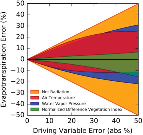
The analysis showed that the greatest disagreement between input forcing arises from choice of net radiation dataset (Badgley et al., 2015; Fisher et al., 2017, 2008). The solar radiation, humidity, air temperature, wind speed, and soil moisture regulate the transfer of water from the land into the air. Information on phenology and vegetation cover is necessary for seasonal dynamics and relative magnitudes of ET fluxes. The evaporative flux in turn modifies the land surface temperature. Fisher et al. (2017) pointed that at the global annual averaged scale, error in ET for the PT-JPL model was highly sensitive to error in radiative (net radiation) and meteorological (water vapor pressure, air temperature) drivers, and somewhat sensitive to vegetation cover and phenology drivers (e.g., NDVI). This sensitivity varies widely in space and time, as well as with the model (see Figure 8).

Figure 8. The error in ET estimates for the PT-JPL model is sensitive to driving variable errors, adopted from Fisher et al., 2017).

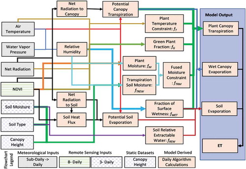
The soil moisture (SM) is an important source of atmospheric water vapor through the ET process, including plant transpiration (T) and bare soil evaporation (E) (see Figure 2). A rich theoretical literature has predicted that SM feedbacks should be more prominent in soil-moisture-limited (Anderegg, Trugman, Bowling, Salvucci, & Tuttle, 2019). The PT-JPL ET model derived from several remote sensing retrieval parameters has outperformed many models for the majority of globally distributed eddy covariance towers within model inter-comparison studies achieving both high explanation of variance and low error (Ershadi et al., 2014; Michel et al., 2016; Vinukollu et al., 2011). However, the PT-JPL algorithm lacks soil moisture control and is restricted by its dependence on a combination of atmospheric conditions and vegetation characteristics to represent surface conditions (Purdy et al., 2018). A PT-JPL_SM algorithm was proposed by Purdy et al. (2018) with incorporating explicit surface soil moisture constraint from SMAP (Soil Moisture Active and Passive, https://smap.jpl.nasa.gov/) satellite to model ET globally. To address previous model parameterization limitations, they use integrated in situ observations of soil moisture and ET to implement soil moisture control within the PT-JPL mode. Figure 9 shows the data processing stream for running PT-JPL _SM model (Purdy et al., 2018).

Figure 9. Flow chart showing data processing stream for the PT-JPL _SM model (Purdy et al., 2018).

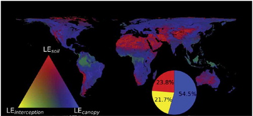
The PT-JPL_SM model improved ET estimates by reducing bias and RMSE by 29.9% and 22.7%, respectively (Purdy et al., 2018). Based on PT-JPL_SM ET estimates, Figure 10 illustrates the fraction of transpiration (T), interception, and soil evaporation (E) globally and each component contribution to mean annual ET. The top map presents the percent contribution from each component and reveals expected global patterns of dominant ET components (e.g. soil E is greatest in deserts, T is dominant in forested regions, and interception is a large fraction in rainforests) (Purdy et al., 2018).

Figure 10. Evapotranspiration components as expressed as a percentage of total ET. Red indicates more soil evaporation, blue indicates more transpiration, yellow indicates more canopy interception evaporation. Below, total contribution to annual ET from transpiration, soil evaporation, and interception (Modified from Purdy et al., 2018).

3.3. Empirical models

The Empirical models are appreciated for their simple construct but limited by its inexplicit physical meaning. Empirical models are always regionally validated. Wang, Wang, Li, Cribb, and Sparrow (2007) proposed a model combining temperature (T₀ or T_s), R_n and VI with a simple construct, such that Equation (14)(14) $ET=R_n\cdot \left(a_0+a_1\cdot VI+a_2\cdot T\right)$(14) :

(14) $ET=R_n\cdot \left(a_0+a_1\cdot VI+a_2\cdot T\right)$(14)

where VI can be EVI (enhanced vegetation index) or NDVI, and T can be daytime-averaged (or daytime maximum) air temperature or T_s (Wang et al., 2007). Equation (14)(14) $ET=R_n\cdot \left(a_0+a_1\cdot VI+a_2\cdot T\right)$(14) is validated on Southern Great Plains, where the main driven forces for ET are available energy, NDVI and air or surface temperature (Wang et al., 2007). But this model would overestimate ET on water deficit surface as it failed to consider the impact of soil moisture (Wang & Liang, 2008; Wang et al., 2007). The SM can substantially affect ET (Gu et al., 2006; Jung et al., 2010; Purdy et al., 2018; Wang et al., 2006), but there is no continuous and reliable daily SM dataset at the resolution consistence with other available RS dataset, e.g., MODIS and AVHRR products (Wang & Liang, 2008). Diurnal land surface or air temperature range (DTsR), by which Equation (14)(14) $ET=R_n\cdot \left(a_0+a_1\cdot VI+a_2\cdot T\right)$(14) is supplemented, was regarded as the substitution for SM on global scale.

Such improvement has significantly reduced the overall RMSE from 34.1$\mathrm{W}/{\mathrm{m}}^2$ produced by the old version to 29.6 $\mathrm{W}/{\mathrm{m}}^2$ produced by the revised version (Wang & Liang, 2008). The reason that DTsR can reflect the soil moisture condition is that dry surface is more easily to be heated, while wet surface is versus. But one should be careful when using DTsR as the substitution of SM. Actually, the DTsR is mainly controlled by both SM and surface global solar radiation $R_g$. To illustrate, assume that there are two positions on the earth with the same underlying surface but with different atmospheric meteorological conditions (sunny day and cloudy day for them, respectively), they will get different $R_g$, which are likely leading to different DTsR for either of the positions. Without considering the impact of SM, for an area limiting region, a simplified relationship between daily $R_g$ and DTsR is found (Allen, 1997; Wu, Liu, & Wang, 2007):

(15) $DTsR=a\cdot {\left(\frac{R_g}{R_e}\right)}^2$(15)

where $R_e$ represents the extra solar radiation for a given day and a given position on the earth. For more accurately reflecting the temporal and spatial variation of SM, DTsR assembly should be normalized by Equation (15)(15) $DTsR=a\cdot {\left(\frac{R_g}{R_e}\right)}^2$(15) before being used. Note that this suggestion is still untested.

Some factors are generalized in empirical models, which will produce certain uncertainties in regional and global applications. Land ET is dominated by transpiration (Cleugh et al., 2007; Jasechko et al., 2013), this sub-component of ET is substantially effected by stomatal conductance ($g_{st}$), which equals the canopy conductance ($G_c$) after multiplying LAI and a coefficient. The modified Penman equation, i.e., PM equation is implemented with$G_c$. For canopies with similar canopy structures, the $G_c$ would differ due to the difference of $g_{st}$. But for empirical models, the canopy conductance is merely related to VI, which may fail in detecting the difference of ET from surface with difference $g_{st}$ value. Empirical models are suggested applying in regional scale, for global scale more factors should be considered.

3.4. Integrated models

Consequently, recent studies have shown that global Penman–Monteith equation-based (PM-based) models poorly simulate water stress when estimating ET in the areas having a Mediterranean climate (AMC). To address this issue, we proposed an integrated approach using precipitation, vertical root distribution (VRD), and satellite-retrieved vegetation information to simulate water stress in a PM-based model (namely, RS-WBPM) (Bai et al., 2017). A multilayer water balance module is employed to simulate the soil water stress factor (SWSF) of multiple soil layers at different depths. The water stress factor (WSF) for surface ET is determined by VRD information and SWSF in each layer.

Additionally, four older PM-based models (PMOV) are evaluated at 27 flux sites in AMC. Results showed that RS-WBPM model can successfully estimate the magnitude or captured the variation of ET in summer at most sites of AMC regions. The RS-WBPM model is also found to outperform other ET models that also incorporate a soil water balance module. As all inputs of RS-WBPM are globally available, the results from RS-WBPM are encouraging and imply the potential of its implementation on a regional or global scale.

Physiologically, in particular, the canopy conductance (G_c), as up-scaled from stomatal conductance (g_st), plays a significant role in regulating ET and photosynthesis (Flexas, Bota, Galmes, Medrano, & Ribas-Carbo, 2006). ET is even directly determined by G_c in arid/semi-arid regions (Zhang, Kadota, Ohata, & Oyunbaatar, 2007), and G_c is an essential input in multiple Earth system models (ESMs) for water (e.g., Yan et al. (2012) and Bai et al. (2017)). Thus, the accurate estimation of G_c is highly important. However, the temporal dynamics of optimum stomatal conductance (g_smax), as well differences between C₃ and C₄ crops, have rarely been considered in previous remote sensing (RS)-based Jarvis-type canopy conductance (G_c) models. Recently, we reported a new RS-based two-leaf Jarvis-type G_c model, RST-G_c, was optimized and validated for C₃ and C₄ crops using 19 crop flux sites across Europe, North America, and China (Bai et al., 2018). The RST- G_c included restrictive functions for T₀, VPD, and soil water deficit, and it used satellite-retrieved NDVI to formulate the temporal variation of g_smax defined at a photosynthetic photon flux density (PPFD) of 2000 μmol m⁻² s⁻¹ (g_{sm, 2000}) (see Figure 11).

Figure 11. Water budget processes of cropland in the RS-WBPM2 model, where F⁽¹⁾ denotes the water infiltrated from the soil surface to soil layer (1), F⁽²⁾ and F⁽³⁾ denote the water percolated from the upper layer to soil layers (2) and (3), respectively, and swl_a ⁽¹⁾, swl_a ⁽²⁾, and swl_a ⁽³⁾ denote the water loss of soil layers (1), (2), and (3), respectively, by transpiration (E_dry ^c) (Bai et al., 2018).

The RST- G_c results indicated that the parameters of RST- G_c differed between C₃ and C₄ crops. The RST- G_c successfully simulated variations in Penman–Monteith (PM)-derived daytime G_c with higher correlations for both C₃ and C₄ crops. Furthermore, the RST- G_c was incorporated into a revised ET model. Hereby, the efforts were made in the revised ET model (denoted as RS-WBPM2), which was modified from the water balance-based RSPM (RS-WBPM) model of Bai et al. (2017). The photosynthesis-based stomatal conductance model, developed by Ball, Woodrow, and Berry (1987). The optimized RST-G_c model was coupled with the RS-WBPM2 model for estimating ET on a daily basis at 19 crop flux sites. The cross validation showed that the modeled daily and 16-day ET of both C₃ and C₄ crops agree well with flux tower data. Inter-site variations in ET were also successfully reproduced by the models. The results implied that the RS-WBPM2 is useful tool for modeling regional or global ET (Bai et al., 2018).

4. Global evapotranspiration estimates and analysis

4.1. Global ET estimation and uncertainty

Estimation of global ET is of great importance for meteorology and climate studies (Fisher et al., 2017, 2011). As mentioned, many efforts have been made to derive this factor with limited meteorological measurement. Some process-based models (including energy balance and Penman–Monteith methods) are appreciated for their global availability without validating, while advantages for empirical models lie in their simplified structure or low requirement for inputs. For recent, some studies global ET produced by various models are summarized in Table 1. Note that not all global ET estimates are included in this summery, for example that derived by LSM (land surface model) (Alton, Fisher, Los, & Williams, 2009; Chen, 2005), since ET models are sub-models in LSMs. But more physiological processes are considered in LSMs, for which LSMs simulation is more close to the work of the true world, so further review is needed.

Table 1. Summarize for the global ET estimates.

No.	Models	Period	Annual $ET$ (${10}^3\mathrm{k}{\mathrm{m}}^3$)	Trend$(\mathrm{m}\mathrm{m}/\mathrm{a})$	Reference
1	Empirical Eq.	1986–1995	47.5$\mathrm{W}/{\mathrm{m}}^2$	-	(Wang & Liang, 2008)
2	MTE	1982–2008	65$\pm$3	1982–1997: 0.71 1998–2008: -0.16 Overall: 0.41	(Jung et al., 2010)
3	Two-Source PM	1984–1998	58.4	1.55	(Yan et al., 2012)
4	Two-Source PM	1982–2011	64.8$\pm$0.8	1982–1997: 0.4 1998–2008: -0.2 Overall: 0.46	(Yan et al., 2013)
5	Semi-Empirical TP	2003–2005	41.7$\mathrm{W}/{\mathrm{m}}^2$	-	(Yao et al., 2015)
6	Two-Source PM	2000–2006	62.8	-	(Mu et al., 2011)
7	Corrected PT	1986–1993	-	$\uparrow$	(Fisher et al., 2008)

Estimate for Global ET varies significantly over different models, several studies made similar reports, e.g., Chen et al. (2014), Mueller et al. (2011), Miralles et al. (2016), Wang and Dickson (2012), Yan et al. (2013). Four results (record No.3-No.6) from process-based models and two (record No.1 & No.2) from empirical models are summarized in Table 1. Two main issues are found: 1) results from the same model driven by different forces datasets are different; Differences exist between meteorological data measured by the tower and that from grid datasets of land meteorology (e.g., ISLSCP-II and GMAO), which lead to different model parameterizations using the kinds of data (Wang & Liang, 2008; Yao et al., 2015). But there are also uncertainties among various meteorological datasets (Talsma et al., 2018a, 2018b).

Yan et al. (2013) estimated global ET from 1982 to 2011 with 6 different precipitation datasets. The slope of each trend line for annual ET anomalies by each precipitation dataset varies from 0.30 to 0.59, while the averaged trend slope is 0.46. Results from different process-based models are different (see Table 1). Large number of factors are evolved in evapotranspiration (Chen et al., 2014; Fisher et al., 2011; Mu et al., 2011), and not all are globally available. Uncertainties among models are largely due to model mechanisms (Fisher et al., 2011). For the first implement of PM model on continental scale, the surface conductance was only related to physical structure of canopy, which lead to overestimate for water stress area (Cleugh et al., 2007). Strategies (records No.3 to 6 in Table 1) are proposed for this issue (Mu et al., 2007, 2011; Yan et al., 2012), but these ways only provide substituting solutions for real required factors since these requirements are not global feasibly, e.g., soil moisture and stomata conductance for different types of plants. Difference between substitutions will introduce more uncertainties to ET estimates.

Empirical models may be good methods for global ET estimates in data limitation era. As shown in Table 1, significant differences are found between global annual ET values by two different empirical models. A comparison study among five empirical models in China shows another problem that the accuracy of empirical models highly depend on the quantity of training samples (Chen et al., 2014). The validated models only explain 55%-averaged variation with 40% data used in training and 61% variation with 80% data for 3 empirical models. So only when enough validating data covering considerable various of ecosystems is available could empirical model be best capable.

4.2. Global ET dynamic

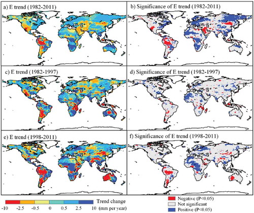
Essentially, land ET, linking atmosphere, vegetation, and soil cycles, is an important component of land water and energy cycles. Global ET consumes more than half of absorbed solar energy and returns about 60% of annual land precipitation to the atmosphere (Oki & Kanae, 2006). To reveal the global ET dynamic is critical for the climate change. Some studies have reported the global ET various in different time periods. Yan et al. (2012) reported that for the global annual ET and ratio of annual ET to annual precipitation averaged from 1984 to 1998, in the major deserts of North Africa, Middle East, Middle Asia, and Australia, almost all precipitation evaporated into the atmosphere. In vegetated regions, annual ET is less than annual precipitation, i.e., precipitation is partly converted into ET, with the residual going to runoff and leakage flow (Yan et al., 2012). During 1982–2011, the ARTS ensemble average ET had an overall increasing trend for most of the global land area while significant decreasing trend still existed in western North America, Amazon, Middle East, Northeast of China, etc. (Figure 12(a,b)). However, during the first period of 1982–1997, most land area shows an insignificant trend of ET (Figure 12(c,d)). Conversely, during the second period of 1998–2011, more land areas (e.g., Australia and Amazon) had a decreasing trend of ET while tropical Africa showed an increasing trend of ET (Figure 12(e,f)) (Yan et al., 2013).

Figure 12. Distribution of global trend of ARTS ensemble average ET and its significance of linear trend for period of (a, b) 1982–2011, (c, d) 1982–1997, and (e, f) 1998–2011, respectively (Yan et al., 2013).

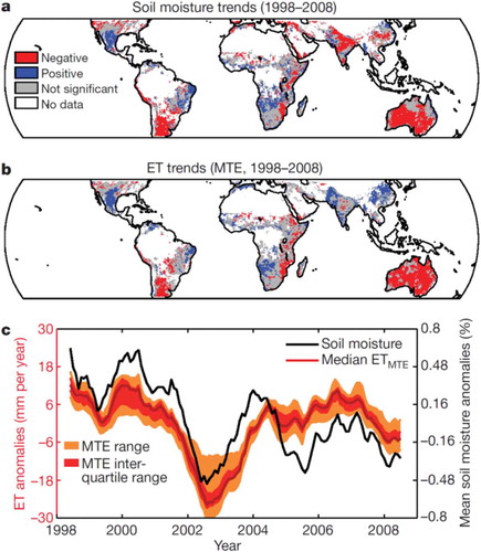
Jung et al. (2010) provided a data-driven estimate of global land ET from 1982 to 2008, compiled using a global monitoring network, meteorological and remote sensing observations, and a machine-learning algorithm. Also, this study assessed ET variations over the same time period using an ensemble of process-based land-surface models. The results suggest that global annual ET increased on average by 7.1+- 1.0 mm per year per decade from1982 to 1997. After that, coincident with the last major El Nin˜o event in 1998, the global ET increase seems to have ceased until 2008 (Figure 13). This change was driven primarily by moisture limitation in the Southern Hemisphere, particularly Africa and Australia. In these regions, microwave satellite observations indicate that soil moisture decreased from 1998 to 2008. Hence, increasing soil-moisture limitations on ET largely explain the recent decline of the global land ET trend. Whether the changing behavior of ET is representative of natural climate variability or reflects a more permanent reorganization of the land water cycle is a key question for earth system science (Jung et al., 2010).

Figure 13. Soil-moisture and ET trends. Significant (P,0.1) soil-moisture trends derived from TRMM (a), significant (P,0.1) ET trends from MTE (b) and mean ET and soil-moisture anomalies (seasonal cycle subtracted and filtered with an 11-month running mean) of all valid pixels of the TRMM domain (c). For consistency and improved comparability, regions without data in either MTE (non-vegetated areas) or TRMM soil-moisture data (very dense vegetation) are blanked in the trend maps of a and b. (Jung et al., 2010).

5. Discussion and conclusion

Modeling evapotranspiration (ET) is of great significant (Fisher et al., 2011; McCabe et al., 2019). The knowledge of ET with spatial scale from field to globe and temporal scale from day to year is essential for water resources management, climatic variations, natural disaster monitoring, and agricultural irrigations (Fisher et al., 2017; Miralles et al., 2011, 2013; Mueller et al., 2011; Tang et al., 2010; Wang et al., 2006; Yao, Liang, Qin, Wang, & Zhao, 2011).

Many field measurement instruments were built to collect this information like the FLUXNET introduced. It is, however, neither economically or logistically possible to build an observation network capable enough to capture global ET (Jiang & Islam, 2001). Coupling which RS information provides alternative ways. The ET models using available RS datasets, which are able to represent the distribution of primary factors (e.g., Albedo, R_n, LAI, VI, fAPAR, SM, and $T_s$) impacting ET, can derive ET pattern globally (Fisher et al., 2008, 2011; Jiménez et al., 2011). We could not construct models as complex as the true world at present, but only find a best one to meet both accurate simulation and data limitation. Various ET models are proposed with different data requirements and mechanisms, and they are of success of different degrees (Badgley et al., 2015; Fisher et al., 2011; Jiménez et al., 2011; McCabe et al., 2019; Stoy et al., 2019).

Source energy balance (SEB) models use surface temperature $T_s$ retrieved from satellites and ground measured meteorology factors to derived energy fluxes of the earth surface. Similar models could be applied without field calibration and are of great potential for regional application due to their physical basis. The SEB models use Monin–Obukhov Similarity Theory (MOST) to calculate$H$, while ET is calculated as the residue of the surface energy budget according to Equation (1)(1) $\lambda E=R_n-H-G$(1) . However, accuracy of satellite retrieved $T_s$ is limited, for which large uncertainties in $H$ estimates are found (Cleugh et al., 2007; Jiang & Islam, 2001; Wang & Dickinson, 2012; Wang & Liang, 2008). Inaccuracy of $T_s$ retrieval is primarily induced by the heterogeneity of the underlying surface. This issue has limited the application of SEB similar methods; it is commonly utilized in homogenous lands.

Compared to the limitation of the SEB model, Penman–Monteith equation and similar ones are more appreciated for its insensitivity to the uncertainty of the input. It is considered to have considerable sound mechanism for ET estimates, and many factors are evolved in PM equation. Surface conductance is a key factor directly related to leaf stomata conductance, which varies among different biomass and is not globally available. Another parameter aerodynamic conductance, which includes the effects of atmosphere condition, is also hard to accurately estimate in global scale (Fisher et al., 2008). Fortunately, studies show that annual variation of global ET is slightly effected by this parameter (Jiang & Islam, 2001). A simplified one for PM equation was the PT equation (Equation (10)(10) $\lambda E=\alpha \frac{\mathrm{\Delta }}{\mathrm{\Delta }+\gamma }\left(R_n-G\right)$(10) ) (Priestley & Taylor, 1972). Though it considers no constrains from the surface and atmosphere, Eichinger, Parlange, and Stricker (1996) showed that PT coefficient $\alpha$ given 1.26 was quite reasonable for equilibrium evaporation wet surface. To reduce equilibrium evaporation to actual evaporation for typical surfaces is the primary work for both PM and PT equations in global application. For recent, several methods to manage this goal have been proposed, but which one could work best on global scale is still unknown. Among them, the $T^{\ast }-VI$ space method is of great potential for its low requirement for inputs; however, several issues should be addressed in global application, such that: 1) The effect of $R_n$ on $T^{\ast }-VI$ space could not be eliminated; 2) Manual determining the cold edge and warm edge is not operational for long-term estimating; 3) This method uses surface $T^{\ast }$ as input, which is an instantaneous parameter, in practice estimated ET should be upscaled to daily value; 4) Application of this method for mix terrain types has not been tested.

Empirical models are embraced for its simplification but its shortage is also obvious. 1) without physical or process basis, temporal and spatial uncertainties are hard to control for empirical models; 2) representativeness of the calibrated model highly depend on the training samples. Semi-empirical models maybe more proper for practice. Methods based on PT equations coupling with empirical corrections are summarized in section 3.2.3. Corrections focused on the atmosphere and surface constraint to evaporation, and constraint factors are core issues.

Nonetheless, to find the most proper way to estimate global ET remains problematic, though many methods have been proposed (Bai et al., 2018; Badgley et al., 2015; Fisher et al., 2008 &, 2011; Mueller et al., 2011; McCabe et al., 2019; Stoy et al., 2019; Yan et al., 2013; Yao et al., 2017). Different results have been reported as shown in Table 1. For regional applications, these models produce even larger differences (Chen et al., 2014). Several reasons have led to the uncertainty among models, such that: 1) Model mechanisms are different, it is impossible for a model to consider all that happen to affect ET, only some key processes are included, and different models are with different considerations. 2) Uncertainties exist in observation data for model validating (McCabe et al., 2019). The flux tower represents a vague domain size, while the pixel on the RS image represents for a typical spatial size. Fluxes observations also have energy unclosed problem for EC towers and observation error less than 20%. 3) Uncertainties exist among different global meteorology datasets. Global distribution datasets of meteorology factors are found to significant different from tower data, also different distribution datasets are different from each other; 4) The limitation of RS techniques has induced considerable uncertainty in underlying surface factors. Due to heterogeneity and BRDF effect of the underlying surface, large uncertainties exist in MODIS global VI and LAI products, which are widely used in macro estimation of ET. These issues need to be addressed, especially the fist one, more processes should be considered but not all. Nevertheless, the similar annual variation trend of global ET is captured by different models (Jung et al., 2010; Wang, Dickinson, Wild, & Liang, 2010b; Yan et al., 2013), which is also of significant meaning for climate change research.

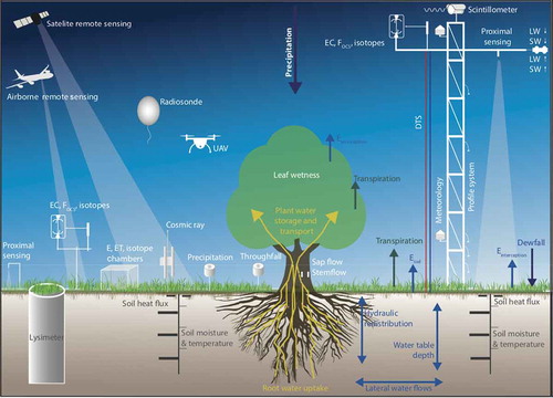
The partitioning of evapotranspiration (ET) is a critical factor in the terrestrial water balance, and understanding the partitioning across terrestrial biomes and the relationships between ET partitions and potential influencing factors is important for predicting future ecosystem feedbacks (Gu et al., 2018). The partitioning of ET in a model between evaporation (E) and transpiration (T) influences its sensitivity to environmental factors. Properly, remote sensing algorithms rely on a process-based understanding of E and T to estimate ET, but it is not clear how to guide their improvement without accurate ground-based E and T observations at spatial scales on the order of a few kilometers or less (Talsma et al., 2018a, 2018b; Stoy et al., 2019), the E and T respond differently to ongoing changes in climate, atmospheric composition, and land use. It is difficult to partition ecosystem-scale ET measurements into E and T, which makes it difficult to validate satellite data (Stoy et al., 2019). Recently, a new measurement technique and analytical approaches for partitioning E and T at the ecosystem scale were proposed by Stoy et al. (2019). The outline of the basics of an ecosystem-scale experiment designed to address uncertainties in E and T measurements is shown in Figure 14 (details see Stoy et al., 2019).

Overall, we have made an overview about the observation, modelling and satellite-based estimation of global terrestrial ET; however, there still insufficient, more aspects related to ET estimates, and the realities, trends, behaviors and constraints of global terrestrial ET that need to be involved in further work.

Figure 14. A schematic of an ecosystem experiment designed to measure transpiration and evaporation from soil and intercepted water using multiple complementary measurement approaches (Stoy et al., 2019).

Acknowledgments

This work was funded by the CAS Strategic Priority Research Program (No. XDA19030402) and the National Natural Science Foundation of China (No. 31671585, 41871253). We are very grateful to the editor and anonymous reviewers for their valuable comments and suggestions.

Disclosure statement

No potential conflict of interest was reported by the authors.

Additional information

Funding

This work was supported by the CAS Strategic Priority Research CAS [No. XDA19030402]; National Natural Science Foundation of China [31671585, 41871253].

Appendix

Table A1. Variables symbol list in this paper.

Variables Symbol	Meanings
ET	Evapotranspiration
AET	Actual evapotranspiration
$\lambda E$	Latent heat flux
$\lambda E_{wet}$	Latent heat without water stress
$\lambda E_c$	Latent heat flux from the vegetation canopy
$\lambda E_s$	Latent heat flux from the soil surface
H	sensible heat flux
G	Ground heat flux
Rn	Surface net radiation
$R_g$	Surface global solar radiation
$R_e$	Extra solar radiation for a given day and a given position on the earth
E	Evaporation
T	Transpiration
Ta	Air temperature
$\mathrm{\Delta }{T}_a$	Vertical air temperature difference
T0	Aerodynamic temperature
Ts	Land surface temperature
$\mathrm{\Delta }{T}_s$	day–night Ts difference
Tc	canopy temperature
$T^{\ast }$	Temperature scale
DTsR	Diurnal land surface or air temperature range
$r_0$	Fractional hemispheric surface reflectance
$r_a$	Aerodynamic resistance
$r_s$	Surface resistance
$r_{bl}$	Boundary layer resistance
$\rho$	Air density
$c_p$	Air constant pressure specific heat
$C$	Regression coefficient related with soil condition
$a$	Regression coefficient
$a_i,i=0,1,\mathrm{2..}n$	Regression coefficient
$b$	Regression coefficient
$K_c$	Ratio of soil heat flux to net radiation for full canopy
$K_s$	Ratio of soil heat flux to net radiation with bare soil
$k{B}^{-1}$	Calculating air resistance to heat transport
$\mathrm{\Delta }$	Water vapor pressure gradient
$\gamma$	Psychrometric constant
${\mathrm{e}}_s$	Saturation vapour pressure
${\mathrm{e}}_a$	Actual water vapor pressure
$\alpha$	Priestley-Taylor coefficient controlled by surface water condition
${\mathrm{g}}_s$	Surface conductance
${\mathrm{c}}_L$	Mean surface conductance per unit leaf area index
${\mathrm{g}}_{s,min}$	Surface conductance controlling soil evaporation and the conductance through the leaf cuticle (Cleugh et al., 2007)
gst	Stomatal conductance
gsmax	Optimum stomatal conductance
$G_c$	Canopy conductance
VPD	Vapor pressure deficit
VI	Vegetation index
$NDVI$	Normalized difference vegetation index
EVI	Enhanced vegetation index
CWSI	Crop water stress index
SAVI	Soil adjusted vegetation index
LAI	Leaf area index
$f\left(C\right)$	Fractional canopy cover
VFC	Vegetation fractional cover
fAPAR	Fraction of Absorbed Photosynthetically Active Radiation
BRDF	Bidirectional Reflectance Distribution Function
RH	Relative humidity
SM	Soil moisture

References

- Allen, R. G. (1997). Self-calibrating method for estimating solar radiation from air temperature. Journal of Hydrological Engineer -ASCE, 2(2), 56–67.
- Allen, R. G., Pereira, L. S., Howell, T. A., & Jensen, M. E. (2011). Evapotranspiration information reporting: I. Factors governing measurement accuracy. Agricultural Water Management, 98(6), 899–920.
- Allen, R. G., Pereira, L. S., Raes, D., & Smith, M. (1998). Crop evapotranspiration-guidelines for computing crop water requirements. FAO Irrigation and Drainage Paper No. 56. Food and Agric. Organ. of the United Nations, Rome. 300 (9), D05109.
- Alton, P., Fisher, R., Los, S., & Williams, M. (2009). Simulations of global evapotranspiration using semiempirical and mechanistic schemes of plant hydrology. Global Biogeochemical Cycles, 23(4). doi:10.1029/2009GB003540
- Anderegg, W. R. L., Trugman, A. T., Bowling, D. R., Salvucci, G., & Tuttle, S. E. (2019). Plant functional traits and climate influence drought intensification and land–atmosphere feedbacks. Proceedings of the National Academy of Sciences, 116(28), 14071–14076.
- Anderson, M. C., Norman, J. M., Diak, G. R., Kustas, W. P., & Mecikalski, J. R. (1997). A two-source time-integrated model for estimating surface fluxes using thermal infrared remote sensing. Remote Sensing of Environment, 60(2), 195–216.
- Anderson, M. C., Norman, J. M., Kustas, W. P., Houborg, R., Starks, P., & Agam, N. (2008). A thermal-based remote sensing technique for routine mapping of land-surface carbon, water and energy fluxes from field to regional scales. Remote Sensing of Environment, 112(12), 4227–4241.
- Badgley, G., Fisher, J. B., Jiménez, C., Tu, K. P., & Vinukollu, R. K. (2015). On uncertainty in global evapotranspiration estimates from choice of input forcing datasets. Journal of Hydrometeorology, 16(4), 1449–1455.
- Bai, Y., Zhang, J., Zhang, S., Koju, U. A., Yao, F., & Igbawua, T. (2017). Using precipitation, vertical root distribution and satellite‐retrieved vegetation information to parameterize water stress in a Penman‐Monteith approach to evapotranspiration modeling under Mediterranean climate. Journal of Advances in Modeling Earth Systems, 9(1), 168–192.
- Bai, Y., Zhang, J., Zhang, S., Yao, F., & Magliulo, V. (2018). A remote sensing-based two-leaf canopy conductance model: Global optimization and applications in modeling gross primary productivity and evapotranspiration of crops. Remote Sensing of Environment, 215, 411–437.
- Ball, J.T., Woodrow, I., & Berry, J. (1987). A model predicting stomatal conductance and its contribution to the control of photosynthesis under different environmental conditions. In J. Biggins (Ed.), Progress in photosynthesis research (pp. 221–224). Netherlands: Springer.
- Bastiaanssen, W. G. M., Menentia, M., Feddesb, R. A., & Holtslagc, A. A. M. (1998a). A remote sensing surface energy balance algorithm for land (SEBAL) 1. Formulation. Journal of Hydrology, 212–213(1–4), 198–212.
- Bastiaanssen, W. G. M., Pelgrum, H., Wang, J. S., Ma, Y. M., Moreno, J. F., Roerink, G. J., & van der Wal, T. (1998b). A remote sensing Surface Energy Balance Algorithm for Land (SEBAL) −2. Validation. Journal of Hydrology, 212–213(1–4), 213–229.
- Center, Oak. (2013). Ridge national laboratory distributed active archive. FLUXNET Maps & Graphics Web Page. Retrieved from http://www.fluxnet.ornl.gov/maps-graphics
- Chen, F. (2005). Variability in global land surface energy budgets during 1987–1988 simulated by an off-line land surface model. Climate Dynamics, 24(7–8), 667–684.
- Chen, Y., Xia, J., Liang, S., Feng, J., Fisher, J. B., Li, X., … Yuan, W. (2014). Comparison of satellite-based evapotranspiration models over terrestrial ecosystems in China. Remote Sensing of Environment, 140, 279–293.
- Cleugh, H. A., Leuning, R., Mu, Q., & Running, S. W. (2007). Regional evaporation estimates from flux tower and MODIS satellite data. Remote Sensing of Environment, 106(3), 285–304.
- Colaizzi, P. D., Kustas, W. P., Anderson, M. C., Agam, N., Tolk, J. A., Evett, S. R., … O’Shaughnessy, S. A. (2012). Two-source energy balance model estimates of evapotranspiration using component and composite surface temperatures. Advances in Water Resources, 50, 134–151.
- Eichinger, W. E., Parlange, M. B., & Stricker, H. (1996). On the concept of equilibrium evaporation and the value of the Priestley-Taylor coefficient. Water Resources Research, 32(1), 161–164.
- Eleanor, B., & John, H. R. (2011). Methods to separate observed global evapotranspiration into the interception, transpiration and soil surface evaporation components. Hydrological Processes, 26, 4063–4068.
- Elhag, M., Psilovikos, A., Manakos, I., & Perakis, K. (2011). Application of the Sebs water balance model in estimating daily evapotranspiration and evaporative fraction from remote sensing data over the Nile Delta. Water Resources Management, 25(11), 2731–2742.
- Ershadi, A., McCabe, M. F., Evans, J. P., Chaney, N. W., & Wood, E. F. (2014). Multi-site evaluation of terrestrial evaporation models using FLUXNET data. Agricultural and Forest Meteorology, 187, 46–61.
- Fang, H., Wei, S., & Liang, S. (2012). Validation of MODIS and CYCLOPES LAI products using global field measurement data. Remote Sensing of Environment, 119, 43–54.
- Fisher, J. B., and ECOSTRESS Algorithm Development Team. (2015). ECOsystem Spaceborne Thermal Radiometer Experiment on Space Station (ECOSTRESS): Level-3 Evapotranspiration LE(ET_PT-JPL) Algorithm Theoretical Basis Document (ATBD) Rep. Pasadena: Jet Propulsion Laboratory, p. 24.
- Fisher, J. B., and ECOSTRESS Algorithm Development Team (2018). ECOsystem Spaceborne Thermal Radiometer Experiment on Space Station (ECOSTRESS): Level-3 Evapotranspiration LE(ET_PT-JPL) Algorithm Theoretical Basis Document (ATBD). ECOSTRESS Science Document no. D-94645. Jet Propulsion Laboratory, Pasadena.
- Fisher, J. B., Lee, B., Purdy, A. J., Halverson, G. H., Cawse-Nicholson, K., Wang, A., & Hook, S. (2020). ECOSTRESS: NASA’s next generation mission to measure evapotranspiration from the International Space Station. Water Resources Research. in press.
- Fisher, J. B., Melton, F., Middleton, E., Hain, C., Anderson, M., Allen, R., & Wood, E. F. (2017). The future of evapotranspiration: Global requirements for ecosystem functioning, carbon and climate feedbacks, agricultural management, and water resources. Water Resources Research, 53(4), 2618–2626.
- Fisher, J. B., Tu, K. P., & Baldocchi, D. D. (2008). Global estimates of the land–atmosphere water flux based on monthly AVHRR and ISLSCP-II data, validated at 16 FLUXNET sites. Remote Sensing of Environment, 112(3), 901–919.
- Fisher, J. B., Whittaker, R. H., & Malhi, Y. (2011). ET Come Home: A critical evaluation of the use of evapotranspiration in geographical ecology. Global Ecology and Biogeography, 20(1), 1–18.
- Flexas, J., Bota, J., Galmes, J., Medrano, H. L., & Ribas-Carbo, M. (2006). Keeping a positive carbon balance under adverse conditions: Responses of photosynthesis and respiration to water stress. Physiologia Plantarum, 127(3), 343–352.
- Foken, T. (2008). The energy balance closure problem: An overview. Ecological Applications, 18(6), 1351–1367.
- French, A. N., Hunsaker, D., Thorp, K., & Clarke, T. (2009). Evapotranspiration over a camelina crop at Maricopa, Arizona. Industrial Crops and Products, 29(2–3), 289–300.
- French, A. N., Hunsaker, D. J., & Thorp, K. R. (2015). Remote sensing of evapotranspiration over cotton using the TSEB and METRIC energy balance models. Remote Sensing of Environment, 158, 281–294.
- Gebler, S., Franssen, H.-J. H., Pütz, T., Post, H., Schmidt, M., & Vereecken, H. (2015). Actual evapotranspiration and precipitation measured by lysimeters: A comparison with eddy covariance and tipping bucket. Hydrology and Earth System Sciences, 19(5), 2145–2161.
- Gharsallah, O., Facchi, A., & Gandolf, C. (2013). Comparison of six evapotranspiration models for a surface irrigated maize agro-ecosystem in Northern Italy. Agricultural Water Management, 130, 119–130.
- Gokmen, M., Vekerdy, Z., Verhoef, A., Verhoef, W., Batelaan, O., & van der Tol, C. (2012). Integration of soil moisture in SEBS for improving evapotranspiration estimation under water stress conditions. Remote Sensing of Environment, 121, 261–274.
- Gu, C., Ma, J., Zhu, G., Yang, H., Zhang, K., Wang, Y., & Gu, C. (2018). Partitioning evapotranspiration using an optimized satellite-based ET model across biomes. Agricultural and Forest Meteorology, 259, 355–363.
- Gu, L., Meyers, T., Pallardy, S. G., Hanson, P. J., Yang, B., Heuer, M., & Wullschleger, S. D. (2006). Direct and indirect effects of atmospheric conditions and soil moisture on surface energy partitioning revealed by a prolonged drought at a temperate forest site. Journal of Geophysical Research, 111(D16). doi:10.1029/2006jd007161
- Halliwell, D. H., & Rouse, W. R. (1987). Soil heat flux in permafrost: Characteristics and accuracy of measurement. Journal of Climatology, 7(6), 571–584.
- Hao, C., Zhang, J., & Yao, F. (2015). Combination of multi-sensor remote sensing data for drought monitoring over Southwest China. International Journal of Applied Earth Observation and Geoinformation, 35, 270–283.
- Hill, M. J., Senarath, U., Lee, A., Zeppel, M., Nightingale, J. M., Williams, R. J., & McVicar, T. R. (2006). Assessment of the MODIS LAI product for Australian ecosystems. Remote Sensing of Environment, 101(4), 495–518.
- Hssaine, B. A., Merlin, O., Rafi, Z., Ezzahar, J., Jarlan, L., Khabba, S., & Er-Raki, S. (2018). Calibrating an evapotranspiration model using radiometric surface temperature, vegetation cover fraction and near-surface soil moisture data. Agricultural and Forest Meteorology, 256–257, 104–115.
- Jackson, R. D., Idso, S. B., Reginato, R. J., & Pinter, P. J. (1981). Canopy temperature as a crop water stress indicator. Water Resources Research, 17(4), 1133–1138.
- Jasechko, S., Sharp, Z. D., Gibson, J. J., Birks, S. J., Yi, Y., & Fawcett, P. J. (2013). Terrestrial water fluxes dominated by transpiration. Nature, 496(7445), 347–350.
- Jiang, C., & Ryu, Y. (2016). Multi-scale evaluation of global gross primary productivity and evapotranspiration products derived from Breathing Earth System Simulator (BESS). Remote Sensing of Environment, 186, 528–547.
- Jiang, L., & Islam, S. (2001). Estimation of surface evaporation map over Southern Great Plains using remote sensing data. Water Resources Research, 37(2), 329–340.
- Jiang, L., Islam, S., Guo, W., Singh, J., Antarpreet, S., Sharika, U. S., … Eltahir, E. (2009). A satellite-based Daily Actual Evapotranspiration estimation algorithm over South Florida. Global and Planetary Change, 67(1–2), 62–77.
- Jiménez, C., Martens, B., Miralles, D. G., Fisher, J. B., Beck, H. E., & Fernández-Prieto, D. (2018). Exploring the merging of the global land evaporation WACMOS-ET products based on local tower measurements. Hydrology and Earth System Sciences, 22(8), 4513–4533.
- Jiménez, C., Prigent, C., Mueller, B., Seneviratne, S. I., McCabe, M. F., Wood, E. F., … Wang, K. (2011). Global inter-comparison of 12 land surface heat flux estimates. Journal of Geophysical Research, 116(D2). doi:10.1029/2010JD014545
- Jin, Y., Randerson, J. T., & Goulden, M. L. (2011). Continental-scale net radiation and evapotranspiration estimated using MODIS satellite observations. Remote Sensing of Environment, 115(9), 2302–2319.
- Jung, M., Reichstein, M., & Bondeau, A. (2009). Towards global empirical upscaling of FLUXNET eddy covariance observations: Validation of a model tree ensemble approach using a biosphere model. Biogeosciences, 6(10), 2001–2013.
- Jung, M., Reichstein, M., Ciais, P., Seneviratne, S. I., Sheffield, J., Goulden, M. L., … Zhang, K. (2010). Recent decline in the global land evapotranspiration trend due to limited moisture supply. Nature, 467(7318), 951–954.
- Jung, M., Reichstein, M., Margolis, H. A., Cescatti, A., Richardson, A. D., Arain, M. A., … Williams, C. (2011). Global patterns of land-atmosphere fluxes of carbon dioxide, latent heat, and sensible heat derived from eddy covariance, satellite, and meteorological observations. Journal of Geophysical Research: Biogeosciences, 116(3), 1–16.
- Komatsu, H., Shinohara, Y., Kume, T., & Otsuki, K. (2008). Relationship between annual rainfall and interception ratio for forests across Japan. Forest Ecology and Management, 256(5), 1189–1197.
- Li, F., & Shen, Y. (2014). Progress in remote sensing-based models for surface heat and water Fluxes. Resources Science, 36(7), 1478–1488. (in Chinese).
- Li, Z., Liu, X., Ma, T., Kejia, D., Zhou, Q., Yao, B., & Niu, T. (2013). Retrieval of the surface evapotranspiration patterns in the alpine grassland–wetland ecosystem applying SEBAL model in the source region of the Yellow River, China. Ecological Modelling, 270, 64–75.
- Masseroni, D., Corbari, C., & Mancini, M. (2014). Limitations and improvements of the energy balance closure with reference to experimental data measured over a maize field. Atmósfera, 27(4), 335–352.
- Masukata, H., Ando, M., & Ogawa, H. (1990). Throughfall, stemflow and interception of rainwater in an evergreen broadleaved forest. Ecological Research, 5(3), 303–316.
- McCabe, M. F., Ershadi, A., Jimenez, C., Miralles, D. G., Michel, D., & Wood, E. F. (2016). The GEWEX LandFlux project: Evaluation of model evaporation using tower-based and globally gridded forcing data. Geoscientific Model Development, 9(1), 283–305.
- McCabe, M. F., Miralles, D. G., Holmes, T. R., & Fisher, J. B. (2019). Advances in the remote sensing of terrestrial evaporation. Remote Sensing, 11(9), 1138. doi:10.3390/rs11091138.
- Merlin, O., Chirouze, J., Olioso, A. T., Jarlan, L., Chehbouni, G., & Boulet, G. (2014). An image-based four-source surface energy balance model to estimate crop evapotranspiration from solar reflectance/thermal emission data (SEB-4S). Agricultural and Forest Meteorology, 184, 188–203.
- Michel, D., Jiménez, C., Miralles, D. G., Jung, M., Hirschi, M., Ershadi, A., … Fernández-Prieto, D. (2016). The WACMOS-ET project–Part 1: Tower-scale evaluation of four remote-sensing-based evapotranspiration algorithms. Hydrology and Earth System Sciences, 20(2), 803–822.
- Miralles, D. G., De Jeu, R. A. M., Gash, J. H., Holmes, T. R. H., & Dolman, A. J. (2011). Magnitude and variability of land evaporation and its components at the global scale. Hydrology and Earth System Sciences, 15(3), 967–981.
- Miralles, D. G., Jiménez, C., Jung, M., Michel, D., Ershadi, A., McCabe, M. F., … Fisher, J. B. (2016). The WACMOS-ET project, part 2: Evaluation of global terrestrial evaporation data sets. Hydrology and Earth System Sciences, 20(2), 823–842.
- Monteith, J. L. (1965). Evaporation and environment. Symposia of the Society for Experimental Biology, 19, 205–224.
- Monteith, J. L. (1995). Accommodation between transpiring vegetation and the convective boundary layer. Journal of Hydrology, 166(3–4), 251–263.
- Mu, Q., Heinsch, F. A., Zhao, M., & Running, S. W. (2007). Development of a global evapotranspiration algorithm based on MODIS and global meteorology data. Remote Sensing of Environment, 111(4), 519–536.
- Mu, Q., Zhao, M., & Running, S. W. (2011). Improvements to a MODIS global terrestrial evapotranspiration algorithm. Remote Sensing of Environment, 115(8), 1781–1800.
- Mueller, B., Hirschi, M., Jimenez, C., Ciais, P., Dirmeyer, P. A., Dolman, A. J., … Seneviratne, S. I. (2013). Benchmark products for land evapotranspiration: LandFlux-EVAL multi-dataset synthesis. Hydrology and Earth System Sciences, 17(10), 3707–3720.
- Mueller, B., Seneviratne, S. I., Jiménez, C., Corti, T., Hirschi, M., Balsamo, G., … Zhang, Y. (2011). Evaluation of global observations-based evapotranspiration datasets and IPCC AR4 simulations. Geophysical Research Letters, 38(6). doi:10.1029/2010GL046230
- Nagler, P. L., Scott, R. L., Westenburg, C., Cleverly, J. R., Glenn, E. P., & Huete, A. R. (2005). Evapotranspiration on western U.S. rivers estimated using the Enhanced Vegetation Index from MODIS and data from eddy covariance and Bowen ratio flux towers. Remote Sensing of Environment, 97(3), 337–351.
- Nassif, D. S. P., Marin, F. R., & Costa, L. G. (2014). Evapotranspiration and transpiration coupling to the atmosphere of Sugarcane in Southern Brazil: Scaling up from leaf to field. Sugar Tech, 16(3), 250–254.
- Norman, J. M., Kustas, W. P., & Humes, K. S. (1995). Source approach for estimating soil and vegetation energy fluxes in observations of directional radiometric surface temperature. Agricultural and Forest Meteorology, 80(2–4), 297.
- Oki, T., & Kanae, S. (2006). Global hydrological cycles and world water resources. Science, 313(5790), 1068–1072.
- Pastorello, G. Z., Papale, D., Chu, H., Trotta, C., Agarwal, D., Canfora, E., … Torn, M. (2017). A new data set to keep a sharper eye on land-air exchanges. EOS, Transactions American Geophysical Union, 98. doi:10.1029/2017EO071597
- Penman, H. L. (1948). Natural evaporation from open water, hare soil and grass. Proceedings of the Royal Society of London. Series A, Mathematical and Physical Sciences, 193(1032), 120–145.
- Penman, H. L. (1956). Evaporation: An introductory survey. Netherlands Journal of Agricultural Science, 4, 7–29.
- Pereira, L. S., Allen, R. G., Smith, M., & Raes, D. (2015). Crop evapotranspiration estimation with FAO56: Past and future. Agricultural Water Management, 147, 4–20.
- Polhamus, A., Fisher, J. B., & Tu, K. P. (2013). What controls the error structure in evapotranspiration models? Agricultural and Forest Meteorology, 169, 12–24.
- Priestley, C. H. B., & Taylor, R. J. (1972). On the assessment of surface heat flux and evaporation using large-scale parameters. Monthly Weather Review, 100(2), 81–92.
- Purdy, A., Fisher, J. B., Goulden, M. L., & Famiglietti, J. S. (2016). Ground heat flux: An analytical review of 6 models evaluated at 88 sites and globally. Journal of Geophysical Research: Biogeosciences, 121(12), 3045–3059.
- Purdy, A. J., Fisher, J. B., Goulden, M. L., Colliander, A., Halverson, G., Tu, K., & Famiglietti, J. S. (2018). SMAP soil moisture improves global evapotranspiration. Remote Sensing of Environment, 219, 1–14.
- Ren, Q., Yang, Z., Li, C., & Zhang, T. (2013). Advances in the study of crop evapotranspiration in changing environment. Advanced Earth Science, 28(11), 1227–1238. (in Chinese).
- Ryu, Y., Baldocchi, D. D., Kobayashi, H., Van Ingen, C., Li, J., Black, T. A., … Roupsard, O. (2011). Integration of MODIS land and atmosphere products with a coupled-process model to estimate gross primary productivity and evapotranspiration from 1 km to global scales. Global Biogeochemical Cycles, 25(4), 1–24.
- Schlesinger, W. H., & Jasechko, S. (2014). Transpiration in the global water cycle. Agricultural and Forest Meteorology, 189–190, 115–117.
- Shao, X., Yao, F., Zhang, J., & Li, X. (2013). Analysis of drought in North China based on evapotranspiration drought index. Meteorological Monthly, 39, 1154–1162.
- Shuttleworth, W. J., & Wallace, J. S. (1985). Evaporation from sparse crops-an energy combination theory. Quarterly Journal of the Royal Meteorological Society, 111(469), 839–855. 551.573:551.584.4:556.132.6.
- Silva, I. C., & Okumura, T. (1996). Throughfall, stemflow and interception loss in a mixed white oak forest (Quercus serrata Thunb.). Journal of Forest Research, 1(3), 123–129.
- Stoy, P. C., El-Madany, T. S., Fisher, J. B., Gentine, P., Gerken, T., Good, S. P., … Wolf, S. (2019). Reviews and syntheses: Turning the challenges of partitioning ecosystem evaporation and transpiration into opportunities. Biogeosciences, 16(19), 3747–3775.
- Su, Z. (2001). A surface energy balance model for estimation of turbulent heat fluxes from point to continental scale. In Su & Jacobs (Eds.), Advanced Earth observation-land surface climate (Vol. UPS-2, pp. 184). Netherlands: Publications of the National Remote Sensing Board (BCRS).
- Su, Z. (2002). The Surface Energy Balance System (SEBS) for estimation of turbulent heat fluxes. Hydrology and Earth System Sciences, 6(1), 85–100.
- Talsma, C. J., Good, S. P., Jimenez, C., Martens, B., Fisher, J. B., Miralles, D. G., & Purdy, A. J. (2018b). Partitioning of evapotranspiration in remote sensing-based models. Agricultural and Forest Meteorology, 260–261, 131–143.
- Talsma, C. J., Good, S. P., Miralles, D. G., Fisher, J. B., Martens, B., Jimenez, C., & Purdy, A. J. (2018a). Sensitivity of evapotranspiration components in remote sensing-based models. Remote Sensing, 10(10), 1601.
- Tang, R., Li, Z., & Tang, B. (2010). An application of the Ts–VI triangle method with enhanced edges determination for evapotranspiration estimation from MODIS data in arid and semi-arid regions: Implementation and validation. Remote Sensing of Environment, 114(3), 540–551.
- Twine, T. E., Kustas, W. P., Norman, J. M., Cook, D. R., Houser, P. R., Meyers, T. P., … Wesely, M. L. (2000). Correcting eddy-covariance flux underestimates over a grassland. Agricultural and Forest Meteorology, 103(3), 279–300.
- Valayamkunnath, P., Sridhara, V., Zhao, W., & Allen, R. G. (2018). Intercomparison of surface energy fluxes, soil moisture, and evapotranspiration from eddy covariance, large-aperture scintillometer, and modeling across three ecosystems in a semiarid climate. Agricultural and Forest Meteorology, 248, 22–47.
- Vinukollu, R. K., Wood, E. F., Ferguson, C. R., & Fisher, J. B. (2011). Global estimates of evapotranspiration for climate studies using multi-sensor remote sensing data: Evaluation of three process-based approaches. Remote Sensing of Environment, 115(3), 801–823.
- Wallace, J., Macfarlane, C., McJannet, D. E., Ellis, T., Grigg, A., & van Dijk, A. (2013). Evaluation of forest interception estimation in the continental scale Australian Water Resources Assessment – Landscape (AWRA-L) model. Journal of Hydrology, 499, 210–223.
- Wang, K., & Dickinson, R. E. (2012). A review of global terrestrial evapotranspiration: Observation, modeling, climatology, and climatic variability. Reviews of Geophysics, 50(2). doi:10.1029/2011rg000373
- Wang, K., Dickinson, R. E., Wild, M., & Liang, S. (2010a). Evidence for decadal variation in global terrestrial evapotranspiration between 1982 and 2002: 1. Model development. Journal of Geophysical Research, 115(D20). doi:10.1029/2009jd013671
- Wang, K., Dickinson, R. E., Wild, M., & Liang, S. (2010b). Evidence for decadal variation in global terrestrial evapotranspiration between 1982 and 2002: 2. Result. Journal of Geophysical Research. doi:10.1029/2010JD013847
- Wang, K., Li, Z., & Cribb, M. (2006). Estimation of evaporative fraction from a combination of day and night land surface temperatures and NDVI: A new method to determine the Priestley–Taylor parameter. Remote Sensing of Environment, 102(3–4), 293–305.
- Wang, K., & Liang, S. (2008). An improved method for estimating global evapotranspiration based on satellite determination of surface net radiation, vegetation index, temperature, and soil moisture. Journal of Hydrometeorology, 9(4), 712–727.
- Wang, K., Wang, P., Li, Z., Cribb, M., & Sparrow, M. (2007). A simple method to estimate actual evapotranspiration from a combination of net radiation, vegetation index, and temperature. Journal of Geophysical Research, 112(D15). doi:10.1029/2006jd008351
- Wu, G., Liu, Y., & Wang, T. (2007). Methods and strategy for modeling daily global solar radiation with measured meteorological data – A case study in Nanchang station, China. Energy Conversion and Management, 48(9), 2447–2452.
- Yan, H., & Shugart, H. H. (2010). An air relative-humidity-based evapotranspiration model from eddy covariance data. Journal of Geophysical Research-Atmospheres, 115(D16), D16106.
- Yan, H., Wang, S. Q., Billesbach, D., Oechel, W., Zhang, J. H., Meyers, T., … Scott, R. (2012). Global estimation of evapotranspiration using a leaf area index-based surface energy and water balance model. Remote Sensing of Environment, 124, 581–595.
- Yan, H., Yu, Q., Zhu, Z., Myneni, R. B., Yan, H., Wang, S., & Shugart, H. H. (2013). Diagnostic analysis of interannual variation of global land evapotranspiration over 1982–2011: Assessing the impact of ENSO. Journal of Geophysical Research: Atmospheres, 118(16), 8969–8983.
- Yang, Y., Su, H., Zhang, R., Tian, J., & Li, L. (2015). An enhanced two-source evapotranspiration model for land (ETEML): Algorithm and evaluation. Remote Sensing of Environment, 168, 54–65.
- Yao, W., Han, M., & Xu, S. (2010). Estimating the regional evapotranspiration in Zhalong wetland with the Two-Source Energy Balance (TSEB) model and Landsat7/ETM+ images. Ecological Informatics, 5(5), 348–358.
- Yao, Y., Liang, S., Cheng, J., Liu, S., Fisher, J. B., Zhang, X., … Zhao, S. (2013). MODIS-driven estimation of terrestrial latent heat flux in China based on a modified Priestley–Taylor algorithm. Agricultural and Forest Meteorology, 171–172(187–202). doi:10.1016/j.agrformet.2012.11.016
- Yao, Y., Liang, S., Li, X., Chen, J., Liu, S., Jia, K., … Roupsar, O. (2017). Improving global terrestrial evapotranspiration estimation using support vector machine by integrating three process-based algorithms. Agricultural and Forest Meteorology, 242, 55–74.
- Yao, Y., Liang, S., Li, X., Chen, J., Wang, K., Jia, K., … Roupsard, O. (2015). A satellite-based hybrid algorithm to determine the Priestley–Taylor parameter for global terrestrial latent heat flux estimation across multiple biomes. Remote Sensing of Environment, 165, 216–233.
- Yao, Y., Liang, S., Qin, Q., Wang, K., & Zhao, S. (2011). Monitoring global land surface drought based on a hybrid evapotranspiration model. International Journal of Applied Earth Observation and Geoinformation, 13(3), 447–457.
- Zhang, J., Fu, C., & Wang, C. (2000). A study of region crop yield model influenced by water deficit based on remote sensing information and crop photosynthetic physiological characteristic. Chinese Journal of Atmospheric Sciences, 24(5), 683–693.
- Zhang, K., Kimball, J. S., Mu, Q., Jones, L. A., Goetz, S. J., & Running, S. W. (2009). Satellite based analysis of northern ET trends and associated changes in the regional water balance from 1983 to 2005. Journal of Hydrology, 379(1–2), 92–110.
- Zhang, K., Pan, S., Zhang, W., Xu, Y., Cao, L., Hao, Y., & Wang, Y. (2015). Influence of climate change on reference evapotranspiration and aridity index and their temporal-spatial variations in the Yellow River Basin, China, from 1961 to 2012. Quaternary International, 380–381, 75–82.
- Zhang, Y., Kadota, T., Ohata, T., & Oyunbaatar, D. (2007). Environmental controls on evapotranspiration from sparse grassland in Mongolia. Hydrological Processes, 21(15), 2016–2027.