
 ?Mathematical formulae have been encoded as MathML and are displayed in this HTML version using MathJax in order to improve their display. Uncheck the box to turn MathJax off. This feature requires Javascript. Click on a formula to zoom.
ABSTRACT
This paper describes how a validated semi-empirical, but physiologically based, remote sensing model – Ensemble_all – was up-scaled using MODIS land surface temperature data (MOD11C2), enhanced vegetation indices (MOD13C1) and land-cover data (MCD12C1) to produce a global terrestrial ecosystem respiration data set (Reco) for January 2001–December 2010. The temporal resolution of this data set is 1 month, the spatial resolution is 0.05°, and the range is from 55°S to 65°N and 180°W to 180°E (crop and natural vegetation mosaic is not included). After cross-validating our data set using in-situ observations as well as Reco outputs from an empirical variable_Q10 model, a LPJ_S1 process model and a machine learning method model, we found that our data set performed well in detecting both temporal and spatial patterns in Reco’s simulation in most ecosystems across the world. This data set can be found at http://www.dx.doi.org/10.11922/sciencedb.934.
1. Introduction
Terrestrial ecosystem respiration (Reco) is an important contributor to climate change (Le Quéré et al., Citation2009). However, the temporal and spatial patterns of Reco are so far poorly understood due to the complex interactions between physical, chemical, and biological factors during the process of respiration (Cramer et al., Citation2001).
MODIS products with weekly 1 km resolution backed by FLUXNET data form an important approach for up-scaling site in situ observations to the global scale. The feasibility of semi-empirical models for simulating FLUXNET Reco at the site scale has been proven (Migliavacca et al., Citation2011; Reichstein et al., Citation2007). Besides, readily available MODIS products showed strong correlations with Reco (Huang & Niu, Citation2013). Reco was often linked to temperature only, without accounting for plant productivity or soil moisture limitations (Schubert, Eklundh, Lund, & Nilsson, Citation2010). Other studies advanced Reco estimates by additional account for plant productivity through vegetation indices (Loranty et al., Citation2011). In addition, Kimball et al. (Citation2009) estimated net carbon fluxes with a process model using satellite microwave temperature and moisture data. Jung, Reichstein, and Bondeau (Citation2009) trained a model tree ensemble to operationally predict GPP and Reco at the global scale, which greatly advanced Reco estimates at global scale by FLUXNET up-scaling. Jägermeyr et al. (Citation2014) proposed a simple RECO model which is capable of up-scaling flux site observations to continental scale based only on MODIS enhanced vegetation indices (EVI) and land surface temperature (LST), but this is mostly an empirical method which lacks physiological basis, especially in the process of simulating reference respiration.
Using flux observations from 171 flux sites (a total of 812 site-years), Ai, Jia, and Epstein et al. (Citation2018) compared six models and found that the Global Polynomial Model (GPM) and Extended Arrhenius model (ETA) were better able to detect the seasonal patterns in Reco. Using MODIS variables and in-situ Reco data, Ai et al. (Citation2018) found that two variables (EVI_LSTnight_mean – the EVI data corresponding to the mean annual night-time LST, LSTnight_min – minimum annual night-time LST), were highly correlated with Rref at the annual mean night-time land surface temperature (Rref, Tref = LSTnight_mean). By also incorporating an EVI_scalar to represent the effect of vegetation change on Reco, these researchers finally developed a semi-empirical, physiologically based remote sensing model – Ensemble_all – which proved to be successful at representing the seasonal and spatial dynamics of Reco.
Up-scaling field-measured respiration data using remote sensing information is an important way of enriching large-scale Reco data sets so that temporal and spatial patterns in the data can be cross-validated (Boulton, Citation2018). Using the above-mentioned Ensemble_all and its corresponding parameters, we up-scaled Ensemble_all using MODIS land surface temperature data (MOD11C2), enhanced vegetation index data (MOD13C1) and land-cover data (MCD12C1_IGBP) and produced a global, terrestrial Reco data set for the period January 2001–December 2010 (Reco_2001_2010_data_set). The temporal resolution of this data set was 1 month and the spatial resolution was 0.05°. The data set covered the ranges 55°S to 65°N and 180°W to 180°E; it did not include the class “crop and natural vegetation mosaic”.
We conducted cross-validation of our data set using in-situ observations and the Reco outputs from the variable_Q10 model proposed by Yuan, Luo, and Li et al. (Citation2011), from the process model LPJ_S1 and from a machine learning data set proposed by Jung et al. (Citation2019) so as to: (1) see if our data set could detect the main temporal and spatial dynamics of Reco in all major ecosystems; and (2) find the regions where our data set and the other three data sets diverge and to explore the reasons behind this divergence.
2. Methods
In the Ensemble_all model, the most efficient model for ecosystems ENF, MF, OSH, GRA, Wet and CRO is ETA-based (EquationEquation 1(1)
(1) ), and the most efficient model for ecosystems EBF, DNF, DBF, CSH, SAV and WSA is GPM-based (EquationEquation 2
(2)
(2) ).
In EquationEquation 1(1)
(1) and EquationEquation 2
(2)
(2) , P1, P2, P3, P4, B and C are parameters, LSTnight_min is the annual minimum night-time land surface temperature, EVI_LSTnight_mean is the EVI value corresponding to the annual mean night-time land surface temperature, and the reference temperature is the annual mean night-time land surface temperature (for more details, see Ai et al. (Citation2018)).
MODIS land surface temperature (MOD11C2), enhanced vegetation index (MOD13C1) and land-cover data (MCD12C1) for 2001 to 2010 were downloaded from the NASA’s Earth Observing System Data and Information System (https://search.earthdata.nasa.gov). In making the global estimates of Reco, quality control flags were examined to screen and reject data that were of insufficient quality. For example, night-time LST data that had an average error >3 K were removed. The land-cover data were filtered using the quality assessment flag (confidence >50%). EVI data that were covered with snow, ice, or clouds were removed; all data that had values outside of valid ranges were also removed. Using these pre-processed data together with the Ensemble_all model, the Reco_2001_2010_data_set was produced.
Using the Reco_2001_2010_data_set, we analyzed the spatial and temporal patterns in Reco. We compared the temporal patterns with site in situ observations (167 sites, a total of 755 site-years) for the major ecosystems (for site information, please check in Ai et al. (Citation2018)); we also explored the seasonal dynamics of the spatial distribution of Reco and the annual global distribution of Reco.
Table 1. Values of the parameters in the Ensemble_all model for each ecosystem.
LPJ_S1 is a widely used and validated process model suitable for the simulation of Reco; it is based on soil parameters and climate inputs only (Sitch et al., Citation2003). Directly coupled with the dynamics of vegetation, temperature and water, the Reco in LPJ_S1 is represented mechanistically (Sitch et al., Citation2008).
Using 276 site-years of eddy co-variance data, Yuan et al. (Citation2011) found that respiration rates at the mean annual temperature (Rref) were closely correlated with mean annual gross primary production (GPP). By using a global annual GPP product and a variable Q10 map derived from a process-based terrestrial model (Zhou, Shi, Hui, & Luo, Citation2009), they estimated the global spatial pattern of Reco for 2000 to 2003.
Jung et al. (Citation2009) proposed a model tree ensemble based on machine learning method (MLM). This method makes extensive use of various meteorological data, remote sensing data, and flux data to optimally integrate model branches and weights. Using this model tree ensemble, they estimated the global energy, carbon and water fluxes from 2001 to 2015 (Jung et al., Citation2019, Citation2020). At present the respiration-controlling mechanism is not yet clear; however, the MLM does not need it, so the MLM could incorporate as much information inside as possible.
We downloaded the Reco outputs from LPJ_S1, from Yuan et al. (Citation2011) and Jung et al. (Citation2019) and compared the annual Reco distributions from the Reco_2001_2010_data_set with the outputs from the three sources. In the areas where the annual Reco patterns in these four sources are highly divergent, we used typical site observations from within these areas and compared them with Reco from the Reco_2001_2010_data_set. The purpose of the comparison was to gain confidence in the approach for regions where the data agree, and also to identify regions of uncertainty.
Finally, we compared the Reco data from these four sources across different latitudes and ecosystems. From the latitudinal distributions, we found out in which latitudinal ranges the values of Reco from the four sources were consistent and for which the uncertainty was low and, conversely, in which latitudinal ranges the data diverged and the uncertainty was large. We obtained similar information from the comparison across different ecosystems.
Statistics include the coefficient of determination (R2), root mean square error (RMSE), modeling efficiency (EF), and mean bias error (MBE):
where the xi are the observed data, yi are the simulated data, and x- and y- are the averages of the observed and simulated data, respectively. R2 represents the fraction of the variation in the observed data that can be explained by these models. RMSE values are used to measure the biases that cause the simulated data to differ from the observations. EF represents the consistency of the observed values with the simulated values and is sensitive to the systematic deviation. EF can range from -∞ to 1. An efficiency of 1 (EF = 1) corresponds to a perfect match between the simulated data and the observed data; the larger the EF value, the better the model. MBE is a bias index; the smaller the MBE, the better the model.
3. Data records
This data set is deposited at http://www.dx.doi.org/10.11922/sciencedb.934. There is a total of 10 zip files, which are named ‘result2001ʹ, ‘result2002ʹ, ‘result2003ʹ, ‘result2004ʹ, ‘result2005ʹ, ‘result2006ʹ, ‘result2007ʹ, ‘result2008ʹ, ‘result2009ʹ and ‘result2010ʹ, and correspond to the terrestrial ecosystem respiration data for 2001 to 2010. Each zip file contains 12 tiff files, one for each month from January to December, each with a spatial resolution of 0.05°. For example, in the zip file ‘result2001ʹ, tiff file number 0 corresponds to the Reco map for January 2001, tiff file number 1 corresponds to the Reco map for February 2001, and so on with the final tiff file (number 11) corresponding to the Reco map for December 2001. The spatial range of each tiff file is from 55°S to 65°N and 180°W to 180°E (the crop and natural vegetation mosaic is not included). The unit used for the data in these tiff files is gCm−2.
4. Technical validation
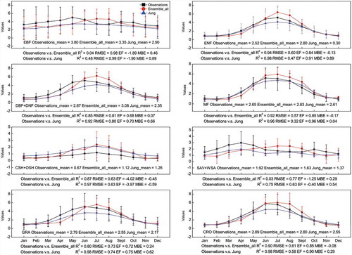
By comparing our data set with the site observations and with the output of Jung et al. (Citation2019), we found that our data set showed high consistency with the site observations, and that our data set was also very similar with the result of Jung et al. (Citation2019) (see ). Although the Reco data in Ensemble_all and Jung et al. (Citation2019) exhibited certain differences in some ecosystems such as the ever-green broad leaved forest (EBF), the closed shrubland and the open shrubland (CSH+OSH) (15 sites, 50 site-years), the savannah and the woody savannah (SAV+WSA) (5 sites, 23 site-years), Reco from our data set and Jung’s both successfully depicted the seasonal patterns in most major ecosystems, especially in the ecosystems such as the evergreen needle-leaved forest (ENF) (39 sites, 185 site-years), the deciduous needle-leaved forest and the deciduous broad-leaved forest (DNF+DBF) (25 sites, 120 site-years), the mixed forest (MF) (6 sites, 31 site-years), the grassland (GRA) (39 sites, 172 site-years), and the cropland (CRO) (27 sites, 105 site-years). Besides, the result from Jung et al. (Citation2019) generally showed a slightly higher consistency with the site observations than our data did. The result from our data set is generally higher than the site observations, while that from Jung et al. (Citation2019) is generally lower than the site observations.
Figure 1. Comparison of Reco data from Reco_2001_2010_data_set, from Jung et al. (Citation2019) and site observations for major ecosystems; unit: gCm−2d−1.
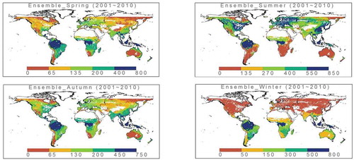
The spatial–seasonal patterns in Reco seen in the Reco_2001_2010_data_set showed that the major seasonal change occurs mainly in the higher-latitude regions of the northern hemisphere, where the highest respiration rate in the summer season is several times higher than that in the winter season (see ). Generally speaking, the seasonality in the northern hemisphere is stronger than that in the southern hemisphere, and it is especially obvious in western Europe, southeastern China and southeastern America, where monsoon forests dominate. In most parts of the southern hemisphere, Reco is high all year round, especially in the rainforest regions; however, in arid central Australia, Reco is low all year round. These findings suggest that this global Reco data set successfully depicts the large-scale spatial seasonality.
Figure 2. Seasonal Reco patterns from Reco_2001_2010_data_set (unit: gCm−2). Spring: March, April and May; Summer: June, July and August; Autumn: September, October and November; Winter: December, January and February. The largest seasonal change occurs in the northern hemisphere.
From 2001 to 2010, the annual average value of global Reco obtained from our data set is 95.38 ± 0.6 PgCa−1: the minimum value is 94.39 Pg, and the maximum value is 96.30 Pg (crop and natural vegetation mosaic is not included). The annual patterns in the Reco_2001_2010_data_set and the other three sources are very similar (see ). The highest annual Reco occurs mainly in the rainforest regions near the equator, followed by western Europe, southeastern China, and southeastern America. The lowest annual Reco occurs mainly in cold regions (high-latitude and high-altitude areas) and arid areas (such as deserts).
After comparing our data set with the outputs of Yuan et al. (Citation2011), LPJ_S1 and Jung et al. (Citation2019), we found that, in most parts of the world, the differences between these four different sources of Reco were relatively small, especially in the arid or cold regions of the northern hemisphere. And especially, our result was very similar with those of Jung et al. (Citation2019) and LPJ_S1.
Figure 3. Annual ecosystem respiration patterns from Reco_2001_2010_data_set, from process model LPJ_S1 and from Jung et al. (Citation2019) (unit: gCm−2a−1); differences in annual ecosystem respiration patterns between Reco_2001_2010_data_set and Yuan et al. (Yuan et al., Citation2011) (Unit: gCm−2a−1); differences in annual ecosystem respiration patterns between Reco_2001_2010_data_set and LPJ_S1 (Unit: gCm−2a−1); differences in annual ecosystem respiration patterns between Reco_2001_2010_data_set and Jung et al. (Jung et al., Citation2019) (Unit: gCm−2a−1).
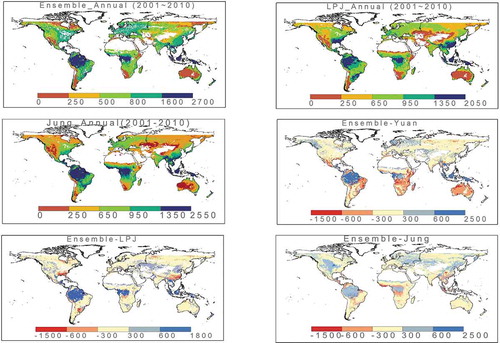
However, in some regions, the differences between the three data sets were large. For example, compared with the other three results, the Reco values in our Reco_2001_2010_data_set were higher in tropical rainforests near the equator, in Mediterranean regions such as central Europe, and in CRO ecosystems such as central and northeast China. Below we listed the regions that exhibited large differences between our result and the other three sources, and we also conducted the comparison between the site in situ observations and our data set (see ). Result showed that in almost all those places where the differences were large, the deviations between the values in the other three data sets and the observed data were greater than the deviations between our data set and the observed ones.
Table 2. The difference between the annual total amount of Reco from Reco_2001_2010_data_set and the flux-measured data at the sites where the difference between the four data sets was the largest (The values in Reco_2001_2010_data_set were closer to the observations than those in the other three data sets (LPJ_S1, Yuan et al. (Citation2011)) and Jung et al. (Citation2019)) were.
The distribution of Reco in each ecosystem from these four data sets was explored (see ). Generally speaking, the patterns in these data sets were very similar: in the ecosystems where the other three data sets exhibited high values, the values in our data set were also high, and in the ecosystems where the other three data sets exhibited low values, our data set had low values, too. However, there were large differences between the values of various ecosystems. For example, the average value of these four data sets in EBF was 4.91, whereas the average value of these four data sets in OSH was 0.82. Among the four data sets, we found that different ecosystems also showed distinct levels of differences. For instance, in EBF, the difference between the four data sets was rather large, while in DBF, the difference between the four data sets was quite small. In addition, we found that in CSH, SAV, MF and ENF, the difference among the four data sets was also large.
Figure 4. Comparison between Reco values for different ecosystems according to the four different data sets (upper); comparisons between the latitudinal distribution of Reco according to the four sources (lower) (negative sign means the North Hemisphere, positive sign means the South Hemisphere).
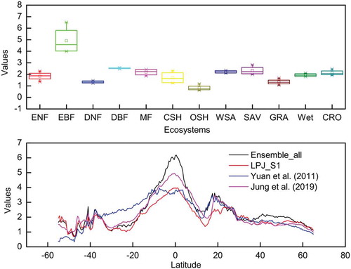
The latitudinal distribution of Reco in these four data sets was also investigated (). In general, the results showed that the latitudinal patterns of Reco in the different data sets were very similar: in low-latitude regions, the values in all three data sets were high and showed a gradual decrease towards higher latitudes. The smallest differences between the data sets occurred between 22°N and 38°N, 1°N and 8°N, and 38°S and 52°S.
At low latitudes (from 5°N to 5°S), the values of Reco in our data set were much higher than those in the other three data sets. In other latitudes – such as between 38°N and 52°N, between 15°N and 28°N, between 35°S and 15°S, below 43°S, and above 53°N – these four data sets were quite different. This reminds us that these places deserve special attention.
5. Data set values
The comparison with the other three data sets showed that the data set produced in this study can powerfully reflect the spatio-temporal dynamics of ecosystem respiration. The distribution pattern of ecosystem respiration in most areas was very similar to the other three data sets, which suggested that the consistency between these models was high in most regions. However, in some regions, the four models differed greatly, especially in EBF and arid areas. This reminds us that in the future, more in-depth research will be needed in these places.
This data set has the following advantages: (1) This data set was developed on the basis of physical processes, and it could powerfully depict the spatial and temporal changes of ecosystem respiration in most ecosystems in the world; (2) This data set used MODIS remote sensing data, thus it was convenient for us to combine with MODIS_GPP data to explore the NEE or NEP process; (3) This data set was an interim result of RECO remote sensing estimation, which could provide valuable information for the future exploration, such as mechanism exploration of Reco in arid regions and EBF ecosystems.
This data sets has the following disadvantages: (1) The accuracy of respiration simulation in arid regions and in EBF needs to be improved; (2) The respiration products provided by the FLUXNET database did not take the photo-respiration and light inhibition process (Keenan et al., Citation2019) into account, which may bias our Reco data set.
Possible application scenarios for this data set include: (1) a combination with MODIS_GPP products to obtain a MODIS_NEE data set (Merritt, Bi, Davis, Windmill, & Xue, Citation2018); and (2) a comprehensive comparison with other ecosystem respiration data sets to reduce the uncertainty in measures of Reco.
Acknowledgments
We are grateful for the freely available MODIS data at https://modis.gsfc.nasa.gov/data/and the flux data at http://www.fluxdata.org/.
Disclosure statement
No potential conflict of interest was reported by the authors.
Data availability statement
The data set is openly available from the Science Data Bank at http://www.dx.doi.org/10.11922/sciencedb.934.
Additional information
Funding
References
- Ai, J., Jia, G., Epstein, H. E., Wang, H., Zhang, A., & Hu, Y. (2018). MODIS-based estimates of global terrestrial ecosystem respiration. Journal of Geophysical Research: Biogeosciences, 123(2), 326–352.
- Boulton, G. (2018). The challenges of a big data earth. Big Earth Data, 2(1), 1–7.
- Cramer, W., Bondeau, A., Woodward, F. I., Prentice, I. C., Betts, R. A., Brovkin, V., … Young-Molling, C. (2001). Global response of terrestrial ecosystem structure and function to CO 2 and climate change: Results from six dynamic global vegetation models. Global Change Biology, 7(4), 357–373.
- Huang, N., & Niu, Z. (2013). Estimating soil respiration using spectral vegetation indices and abiotic factors in irrigated and rainfed agroecosystems. Plant and Soil, 367(1–2), 535–550.
- Jägermeyr, J., Gerten, D., Lucht, W., Hostert, P., Migliavacca, M., & Nemani, R. (2014). A high-resolution approach to estimating ecosystem respiration at continental scales using operational satellite data. Global Change Biology, 20(4), 1191–1210.
- Jung, M., Koirala, S., Weber, U., Ichii, K., Gans, F., Camps-Valls, G., … Reichstein, M. (2019). The FLUXCOM ensemble of global land-atmosphere energy fluxes. Scientific Data, 6(1), 1–14.
- Jung, M., Reichstein, M., & Bondeau, A. (2009). Towards global empirical upscaling of FLUXNET eddy covariance observations: Validation of a model tree ensemble approach using a biosphere model. Biogeosciences, 6(10), 2001–2013.
- Jung, M., Schwalm, C., Migliavacca, M., Walther, S., Camps-Valls, G., Koirala, S., … Reichstein, M. (2020). Scaling carbon fluxes from eddy covariance sites to globe: Synthesis and evaluation of the FLUXCOM approach. Biogeosciences, 17(5), 1343–1365.
- Keenan, T. F., Migliavacca, M., Papale, D., Baldocchi, D., Reichstein, M., Torn, M., & Wutzler, T. (2019). Widespread inhibition of daytime ecosystem respiration. Nature Ecology & Evolution, 3(3), 407–415.
- Kimball, J. S., Jones, L. A., Member, S., Heinsch, F. A., McDonald, K. C., & Oechel, W. C. (2009). A satellite approach to estimate land–atmosphere CO2 exchange for boreal and arctic biomes using MODIS and AMSR-E. Transactions on Geoscience and Remote Sensing, 47(2), 569–587.
- Le Quéré, C., Raupach, M. R., Canadell, J. G., Marland, G., Bopp, L., Ciais, P., & Woodward, F. I. (2009). Trends in the sources and sinks of carbon dioxide. Nature Geoscience, 2(12), 831–836.
- Loranty, M. M., Goetz, S. J., Rastetter, E. B., Rocha, A. V., Shaver, G. R., Humphreys, E. R., & Lafleur, P. M. (2011). Scaling an instantaneous model of tundra NEE to the arctic landscape. Ecosystems, 14(1), 76–93.
- Merritt, P., Bi, H., Davis, B., Windmill, C., & Xue, Y. (2018). Big earth data: A comprehensive analysis of visualization analytics issues. Big Earth Data, 2(4), 321–350.
- Migliavacca, M., Reichstein, M., Richardson, A. D., COLOMBO, R., SUTTON, M. A., LASSLOP, G., & Van Der MOLEN, M. K. (2011). Semiempirical modeling of abiotic and biotic factors controlling ecosystem respiration across eddy covariance sites. Global Change Biology, 17(1), 390–409.
- Reichstein, M., Ciais, P., Papale, D., VALENTINI, R., RUNNING, S., VIOVY, N., … ZHAO, M. (2007). Reduction of ecosystem productivity and respiration during the European summer 2003 climate anomaly: A joint flux tower, remote sensing and modelling analysis. Global Change Biology, 13(3), 634–651.
- Schubert, P., Eklundh, L., Lund, M., & Nilsson, M. (2010). Estimating northern peatland CO2 exchange from MODIS time series data. Remote Sensing of Environment, 114(6), 1178–1189.
- Sitch, S., Huntingford, C., Gedney, N., LEVY, P. E., LOMAS, M., PIAO, S. L., & WOODWARD, F. I. (2008). Evaluation of the terrestrial carbon cycle, future plant geography and climate-carbon cycle feedbacks using five Dynamic Global Vegetation Models (DGVMs). Global Change Biology, 14(9), 2015–2039.
- Sitch, S., Smith, B., Prentice, I. C., Arneth, A., Bondeau, A., Cramer, W., … Venevsky, S. (2003). Evaluation of ecosystem dynamics, plant geography and terrestrial carbon cycling in the LPJ dynamic global vegetation model. Global Change Biology, 9(2), 161–185.
- Yuan, W., Luo, Y., Li, X., Yu, G., Zhou, T., Bahn, M., ... Stoy P. (2011). Redefinition and global estimation of basal ecosystem respiration rate. Global Biogeochemical Cycles, 25(4), GB4002.
- Zhou, T., Shi, P., Hui, D., & Luo, Y. (2009). Global pattern of temperature sensitivity of soil heterotrophic respiration (Q10) and its implications for carbon-climate feedback. Journal of Geophysical Research, 114(G2), G02016.