A 100 m population grid in the CONUS by disaggregating census data with open-source Microsoft building footprints

ABSTRACT

In the Big Data era, Earth observation is becoming a complex process integrating physical and social sectors. This study presents an approach to generating a 100 m population grid in the Contiguous United States (CONUS) by disaggregating the US census records using 125 million of building footprints released by Microsoft in 2018. Land-use data from the OpenStreetMap (OSM), a crowdsourcing platform, was applied to trim original footprints by removing the non-residential buildings. After trimming, several metrics of building measurements such as building size and building count in a census tract were used as weighting scenarios, with which a dasymetric model was applied to disaggregate the American Community Survey (ACS) 5-year estimates (2013–2017) into a 100 m population grid product. The results confirm that the OSM trimming process removes non-residential buildings and thus provides a better representation of population distribution within complicated urban fabrics. The building size in the census tract is found in the optimal weighting scenario. The product is 2.5Gb in size containing 800 million populated grids and is currently hosted by ESRI (http://arcg.is/19S4qK) for visualization. The data can be accessed via https://doi.org/10.7910/DVN/DLGP7Y. With the accelerated acquisition of high-resolution spatial data, the product could be easily updated for spatial and temporal continuity.

KEYWORDS:

• Population census
• high resolution population grid
• microsoft building footprints
• OpenStreetMap
• dasymetric mapping
• CONUS

1. Introduction

Knowing where people live at the local level is essential for a broad range of studies such as disaster responses and damage assessments (Nadim, Kjekstad, Peduzzi, Herold, & Jaedicke, 2006), humanitarian relief operations (Ahola, Virrantaus, Krisp, & Hunter, 2007), public health (Linard, Alegana, Noor, Snow, & Tatem, 2010), resource management, and urban planning (Smith, Nogle, & Cody, 2002). In the United States, official population data is repetitively released by the US Census Bureau. The decennial census records and the American Community Survey (ACS) estimates, for example, have been commonly utilized at different geographical levels and temporal intervals. Population, as a fundamental agent in urban and suburban ecosystems, is distributed with great heterogeneity on Earth surfaces (Li & Zhou, 2018). When utilizing the census data, however, we have to assume a uniform distribution of population within the predefined unit such as census block, block group, and census tract (Wardrop et al., 2018). The spatial dynamics of population within the unit are thus lost, especially in large polygons such as rural areas. In addition, the discontinuity caused by the artifact of underlying statutory boundaries often raises the Modifiable Areal Unit Problem (MAUP) (Fotheringham & Wong, 1991). Boundaries of survey units may also change in different years (Li & Zhou, 2018), which introduces further uncertainties when population data from different survey periods are applied.

To overcome the limitations of the aggregated census data, studies have been conducted to generate spatially continuous population representation, that is, population grid. Dasymetric mapping is the most commonly adopted method to obtain population in each grid cell (Eicher & Brewer, 2001), in which thematic layers at finer scales are used to refine the geographical representation of a quantitative variable at coarse scales. Leyk et al. (2019) recently reviewed a number of large-scale population grid products developed in past years. As summarized in Table 1, the Gridded Population of the World (GPW) is merely based on an areal-weighting approach in population disaggregation. The Global Human Settlement-Population (GHS-POP) uses Landsat-extracted urban areas to disaggregate population in a binary dasymetric method. The LandScan Global Population takes advantage of multiple environmental variables such as land cover/use, slope, settlement locations, and distance to roads to build the weighting layer for disaggregation. The Global Rural-Urban Mapping Project (GRUMP) utilizes nighttime light data in the disaggregating process thanks to their high correlation with human activity. Other variables that are closely related to population patterns have also been explored. For example, the History Database of the Global Environment (HYDE) collects historical population and agricultural data. More detailed methods and references of these products are listed in Table 1.

Table 1. Summary of existing population grid products in different geographic regions

Grid population datasets	Grid size	Location(s) and year(s) represented	Input variable(s)	Methods	Source
History Database of the Global Environment (HYDE) Population Grids, version 3.1 (Klein Goldewijk, Beusen, Van Drecht, & De Vos, 2011)	5 arc-minutes (10 km)	Global, 10,000 BC to 2000 AD	Historical population, croplands, and pasture	Spatially explicit allocation mapping.	Netherlands Environmental Assessment Agency (PBL)
Gridded Population of the World (GPW), version 4 (latest version) (Doxsey-Whitfield et al., 2015)	30 arc-seconds (1 km)	Global, 2000, 2005, 2010, 2015, 2020	Census population, protected areas, water bodies	Areal weighting method that assumes population is uniformly distributed for habitable cells covering census units.	Center for International Earth Science Information Network (CIESIN), Columbia University
Global Rural Urban Mapping Project (GRUMP) (Balk et al., 2006)	30 arc-seconds (1 km)	Global, 1990, 1995, 2000	Census population, protected area, water bodies, urban boundaries, nighttime lights (DMSP)	Binary dasymetric method that uses nighttime lights to allocate population in urban areas.	CIESIN, Columbia University
Global Human Settlement – Population (GHS-POP) (Freire & Pesaresi, 2015)	30 arc-seconds (1 km) and 9 arc-seconds (250 m)	Global 1975, 1990, 2000, 2015	Census population, urban areas from Landsat imagery	Binary dasymetric method that uses Landsat imagery to allocate population in urban areas.	European Commission Joint Research Centre (JRC) and CIESIN, Columbia University
LandScan Global Population Database (Dobson, Bright, Coleman, Durfee, & Worley, 2000)	30 arc-seconds (1 km)	Global, Annual release from 2000–2017 (current)	Census population, roads, land cover, urban areas, environmental variables, water bodies	Dasymetric method that uses land cover, imagery-derived urban areas, and multiple environmental variables to allocate population inhabitable cells.	Oak Ridge National Laboratory (ORNL)
World Population Estimate (WPE) (Frye et al., 2018)	5 arc-seconds (150 m) after 2016, 8 arc-seconds (250 m) before 2016	Global, 2013, 2015, 2016 (current)	Census population, land cover, road, water bodies	Dasymetric method that uses land cover, road density to allocate population inhabitable cells.	ESRI
WorldPop (Tatem, 2017)	30 arc-seconds (1 km) for global mosaic, 3 arc-second (100 m) for all countries in the world	Selected countries (the US excluded), represented year is country-specific	Census population, land cover, roads, urban area, nighttime lights, environment variables, protected areas, water bodies	Dasymetric mapping method that uses statistical weighting layer derived from machine learning approach (Random Forest) to allocate population inhabitable cells	WorldPop
Gridded Population Mapping (Demobase) (Azar, Engstrom, Graesser, & Comenetz, 2013)	3 arc-second (100 m)	Selected countries (Haiti, Pakistan, and Rwanda), represented year is country-specific	Census population, environmental variables, impervious surface from Landsat imagery	Dasymetric mapping method that uses Landsat-derived impervious surface and other environmental variables to allocate population inhabitable cells.	US Census Bureau
High Resolution Settlement Layer (HRSL) (Tiecke et al., 2017)	1 arc-second (30 m)	Selected countries (33 in total, US excluded), 2015	Census population, high resolution imagery (0.5 m) from DigitalGlobe	Binary dasymetric method that uses image-derived building footprints to allocate population in cells with building footprints.	Facebook Connectivity Lab and CIESIN
WSF-POP (Palacios-Lopez et al., 2019)	10 m	Global 2015	Census data, WSF-2015 Layer (binary human settlement layer), WSF-2015-Density (percent impervious surface layer)	Dasymetric mapping method that uses binary human settlement or percent impervious surface to allocate population in habitable cells.	German Aerospace Center (DLR)
OpenPopGrid (Murdock, Harfoot, Martin, Cockings, & Hill, 2015)	10 m	England, UK and Wales, UK, 2011	Census postcode headcounts, postcode centroids, building footprints	Binary dasymetric method that uses building footprints classified by postcode centroid to allocate population in cells with building footprints.	GeoData, University of Southampton

Most of these population products have a grid unit of 30 arc-seconds (approximately 1 km at the equator). Their global coverage provides great efficiency, especially in population studies at regional and global levels. With the growing need for a higher level of geographic precision in population distribution (Frye, Wright, Nordstrand, Terborgh, & Foust, 2018), population grids at sub-km resolution in selected regions and countries started to emerge in recent years (also listed in Table 1). However, similar weighting variables are still in use. For example, the 100 m WorldPop product derives a machine learning-based statistical weighting layer from multiple sources including land cover, roads, nighttime lights, and environmental variables. The 1 km and 150 m World Population Estimate (WPE) products incorporate the distance to road network or identified facilities. Reed, Gaughan, Stevens, and Yetman (2018) compared the population mapping with three high-resolution Built Area products: the 10 m World Settlement Footprint (WSF), 38 m GHS, and 0.5 m HRS. However, the study resampled the fine-scale settlement data into 100 m upon the presence/non-presence of buildings, then established a similar weighting layer by interacting with other environmental variables. Dmowska and Stepinkski (2017) extracted a 30 m population grid for the conterminous United States using the same weighting strategy of Landsat-extracted land use/cover data in the 2011 National Land Cover Database (NLCD) product (Homer et al. 2011). Those methods and variables may not well summarize the population distribution in the grid cell because greater heterogeneity is likely to manifest at a finer scale. It is especially the case in rural areas with low population. Consequently, significant accuracy decay in rural areas has been noted in those products (Tiecke et al., 2017).

To extract population grids at finer scales, there is an urgent need of better weighting variables in large geographic extents to optimally characterize the heterogeneity of population within census units. In the Big Data era, Earth observations have experienced unprecedented advancement in data format, scale, and volume beyond petabyte and exabyte levels across disciplines (Guo, 2017). The WSF-POP is a good example of global mapping in a big data perspective (Palacios-Lopez, Bachofer, Esch, & Heldens, 2019), which utilizes radar and optical imagery (TerraSAR-X/TanDEM-X, Landsat8, and Sentinel) at higher resolutions to deliver the 10 m settlement footprint and population grids. Better accessibility of very high-resolution (VHR, sub-meter) satellite imagery and the surge in research on computer vision have enabled the extraction of individual buildings in a large geographic extent (Yuan, 2018). In June 2018, the Microsoft Bing Maps team released more than 125 million computer-generated building footprints covering all US states from Bing VHR imagery (Microsoft, 2019).

Building footprints could outperform the commonly used weighting variables in population disaggregation. People live in buildings. The distribution of building footprints effectively summarizes the population patterns in both urban and rural areas. More specifically, building statistics such as count and size have stronger linkage to population than other weighting variables such as urban land uses, light intensity, and distance to roads (Small & Nicholls, 2003). The building footprint data has been tested to disaggregate population and proved efficient in capturing the heterogeneity of population patterns at fine scale, for example, the 30 m High-Resolution Settlement Layer (HRSL) and the 10mOpenPopGridextracted from the VHR imagery in selected areas (as listed in Table 1). However, those studies were conducted in small geographical areas. At the time of writing, the Microsoft building footprint product, released in June 2018 and contained a total of 125 million footprints, is believed to be the newest and the most comprehensive building footprints for the entire Contiguous United States (CONUS), which makes it possible to extract high-resolution population grid at a national level.

This study aims to explore the potential of the recently released Microsoft building footprints to create high-resolution population grid for the entire CONUS. As the dwelling unit, building footprints approximate where people live and therefore, are used to disaggregate census tract population in ACS 5-year estimates (2013–2017). This study provides valuable experience of Big Earth Data for studying human settlement with interactive Earth observations in social (census survey) and physical (satellite) sectors. The 100 m population grid delivered in this study could benefit a wide range of studies relying on spatially explicit population data.

2. Datasets

The CONUS covers the 48 contiguous US states and District of Columbia (DC). Three datasets within this region were used in this study: 1) the open-source Microsoft building footprints dataset released in 2018, aiming to generate weighting layers for population disaggregation; 2) the crowdsourced OSM land-use dataset, aiming to trim building footprints to be more relevant to residential population; and 3) the 5-year ACS population estimates (2013–2017) from the US Census Bureau in two unit scales: census tracts and block group. The census tract population is used for the disaggregation process. The block group is the smallest geographical unit of the ACS data. Its population records serve as truthing data to evaluate the extracted population grid.

2.1. Microsoft building footprints

Relying on the open-source Microsoft Cognitive Toolkit (CNTK), in 2018 the Microsoft Bing Maps team released the computer-generated building footprints extracted from Bing imagery within the United States. Trained by 5 million labeled images, the output of building footprints reaches 0.7% commission error and 6.5% omission error (Microsoft, 2019). Given that Bing imagery is a composite of multiple sources, the exact dates of the extracted building footprints are undetermined.

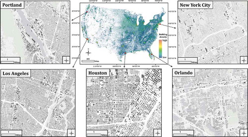
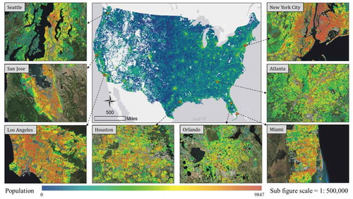
The building footprints used in this study cover the entire CONUS region with a total of 124,828,547 building footprints. We projected the layer into the US Albers equal-area conic projection so that building size can be properly extracted. Individual buildings in five example cities are demonstrated in Figure 1. To acquire a general understanding of their distribution pattern, building density was derived by counting building numbers in each 100 m grid cell within the CONUS (the color map in Figure 1). As expected, urban areas exhibit clusters with higher building count, indicating dense population in urban. A vast building footprint desert is clearly observed in the less populated Mountain States, e.g., Arizona, Colorado, Idaho, Montana, Nevada, New Mexico, Utah, and Wyoming.

Figure 1. Distribution of microsoft building footprints and example sites (grey polygons) in the CONUS

2.2. OSM land use

OpenStreetMap (OSM) is a collaborative project that consists of a very detailed, dynamically updated spatial database of land surface features all over the world from millions of voluntary contributors within an open-source environment (Ramm et al., 2014). The OSM data hosted at GEOFABRIK (https://www.geofabrik.de/geofabrik/) are updated on a daily basis. With the merit of massive, voluntary public participation at a local level, it provides a more detailed and extensive representation of land use on the globe than satellite-based classification (Fonte et al., 2017). The OSM data covering the entire CONUS was downloaded on March 1^st, 2019, which contains a total of 1,714,072 polygons with 19 unique land-use classes (Table 2).

Table 2. OSM land-use statistics in the CONUS

Land-use class	Total records	Total size ($k{m}^2$)	Land-use class	Total records	Total size ($k{m}^2$)
Allotments	1,681	4.52	Industrial	52,537	9,079.45
Commercial	64,216	2,949.86	Meadow	42,615	23,430.72
Farm	186,297	73,989.69	Military	3,124	112,921.92
Forest	358,426	274,690.80	Natural reserve	27,215	683,926.68
Grass	262,348	2,356.47	Orchard	18,259	3583.34
Park	124,472	34,573.64	Quarry	7119	4,197.45
Recreation Ground	21,545	3,238.34	Residential	373,261	42,348.51
Retail	42,913	2,164.11	Scrub	62,416	13,940.30
Vineyard	15,137	1,847.07	Cemetery	45,904	1,529.74
Health	4,587	16,063.60

Note. OSM data used in this study was downloaded on March 1^st, 2019.

2.3. Population dataset

The population dataset was derived from the ACS 5-year estimates by US Census Bureau. The 2013–2017 ACS population data was collected through a 60-month period from Jan 1^st, 2013 to Dec 31^st, 2017. Thanks to its long sampling period, it provides data for the whole CONUS and is believed more reliable compared with those 1-year and 3-year estimates due to the increased statistical reliability, especially when examining very small population within a census unit (ACS, When to Use 1-year, 3-year, or 5-year Estimates, 2018). The CONUS covers 72,538 census tracts and 266,330 block groups in the ACS 5-year product.

3. Methods

3.1. Building footprint trimming

Microsoft building footprints not relevant to the residential population are trimmed in this study. Due to the incomprehensiveness of the residential type in OSM dataset, we did not solely select buildings with a residential type (as shown in Table 2). Instead, building footprints were removed if they were within OSM polygons designated as non-residential types, including allotments, commercial, farm, forest, grass, park, recreation ground, retail, vineyard, health, industrial, meadow, military, natural reserve, orchard, quarry, scrub, and cemetery. Moreover, we observed a wide existence of small footprints that are not likely to be habitable buildings (e.g., garages and trailers) but denoted as “buildings” in the footprints. To remove those small polygons, we set a minimal footprint size of 50 $m^2$. Occasionally, some extra-large footprints such as those associated with commercial and industrial are misclassified as residential in the OSM. We set a maximal footprint size of 5,000 $m^2$. These empirical thresholds are used per our general sense of the abovementioned non-residential units on Google Earth. The trimmed building footprints are then used in the following sections to disaggregate population into finer scales.

3.2. Dasymetric mapping

Dasymetric mapping employs a series of spatial partitions to introduce a higher resolution into a dataset captured at a lower level (Eicher & Brewer, 2001). For population disaggregation, given the known population at source zone $t$($P_t$), the disaggregation process in the whole study region ($R^t)$ follows:

(1) $P_i^e=P_t\times \frac{A_i\times W_i}{{\sum }_i{A}_i\times W_i}\left(iϵR^t\right)$(1)

where $P_i^e$ refers to the estimated population in the target zone$i$. $A_i$ and $W_i$ respectively denote the size of the target zone and the corresponding weight assigned to this zone. The target zone $i$ is within source zone $t$ spatially ($iϵR^t$).

In this study, the source zone is a census tract while the target zone is a 100 m grid cell within the census tract. A centroid rule is applied if a cell is split by two or more tract boundaries, that is, its population is derived from the tract where the cell’s centroid falls. Eq.1(1) $P_i^e=P_t\times \frac{A_i\times W_i}{{\sum }_i{A}_i\times W_i}\left(iϵR^t\right)$(1) partitions the population of a census tract into 100 m cells based on the weighting layer while the sum preserves the original population, i.e., $P_t={\sum }_{iϵR^t}{P}_i^e$. Here, the geospatial layers derived from building footprint statistics define a set of weighting scenarios to disaggregate the ACS population data. The weighting procedure is described in the next section.

3.3. Weighting scenarios

Building footprint-based weighting algorithms were designed to explore its potential in population disaggregation. Positive relationships were assumed between the estimated population and building footprint statistics. Given all trimmed building footprints ($b{f}^{\prime }$) within cell $i$, we calculated three statistics and designed four weighting scenarios:

1. building footprint size (scenario noted as $B{F}_s^{\prime }$), where $W_i=\sum b{f}_s^{\prime }$

2. building footprint count (scenario noted as $B{F}_c^{\prime }$), where $W_i=\sum b{f}_c^{\prime }$

3. building footprint size * count (scenario noted as $B{F}_{sc}^{\prime }$), where $W_i=\sum b{f}_{sc}^{\prime }$

4. a baseline scenario (noted as UNIF) by assuming a uniform distribution of population across each census tract. The population assigned to each cell is proportional to its percentage of coverage in each census tract, i.e., $W_i=\frac{A_i}{{\sum }_i{A}_i}$.

The four weighting scenarios differ in the designated weight of each target cell $i$ (the $W_i$ in Eq.1(1) $P_i^e=P_t\times \frac{A_i\times W_i}{{\sum }_i{A}_i\times W_i}\left(iϵR^t\right)$(1) ). With these scenarios, a total of four 100 m population grid products were extracted with the dasymetric mapping approach.

3.4. Evaluation metrics

Block group is the finest unit of the ACS dataset and its population is assumed ground truth for accuracy assessment. The CONUS population grid in this study is produced by disaggregating population counts at the census tract level. The 100 m grid cells in a census tract are further aggregated to a block group scale to be compared against the ACS population.

Six commonly applied quantitative measurements of accuracy were used to measure the discrepancy between the ACS block group population and the extracted population in the same scale: 1) Root Mean Square Error (RMSE); 2) Mean Absolute Error (MAE); 3) Overall Relative Error (ORE); 4) Coefficient of Efficiency (CoE); 5) Systematic Error (SE) and 6) Modified Index of Agreement (MIoA). RMSE has been widely used to measure the differences between estimated and observed values. MAE is believed to be more robust to outliers than RMSE (Chai & Draxler, 2014). Unlike RMSE and MAE that measure the absolute difference, ORE sheds light on the error rate as its calculation involves percentage difference in each block group. SE calculates the average of all the biases between the estimated and observed values and therefore reveals the existence of systematic bias in the disaggregating method; SE = 0 indicates a perfect disaggregating method without any systematic bias.

Different from the abovementioned error metrics, CoE and MIoA represent an improved agreement evaluation of the commonly used coefficient of determination ($R^2$), which has been criticized by its insensitivity to the proportional difference (Lu, Carbone, & Gao, 2017). Ranging from minus infinity to 1.0, CoE is the proportion of initial variance accounted for by a model (Nash & Sutcliffe, 1970). The higher the CoE value, the better agreement it reaches. MIoA is a modified version of the Index of Agreement (IoA) proposed by Willmott et al. (1985). It ranges from 0 to 1.0 with higher values indicating better agreement. The equations of the six measurements mentioned above are presented in Table 3.

Table 3. Six metrics of statistical measures used for accuracy assessment

Name and abbreviation	Equation
Root mean square error (RMSE)	$RMSE=\sqrt{\frac{{\sum }_{j=1}^n{\left(P_j^e-P_j^g\right)}^2}{n}}$
Mean absolute error (MAE)	$MAE=\frac{{\sum }_{j=1}^n\left|P_j^e-P_j^g\right|}{n}$
Overall relative error (ORE)	$ORE=\frac{{\sum }_{j=1}^n\left|\frac{P_j^e-P_j^g}{P_j^g}\right|}{n}\times 100\mathrm{\%}$
Coefficient of efficiency (CoE)	$CoE=1-\frac{{\sum }_{j=1}^n{\left(P_j^g-P_j^e\right)}^2}{{\sum }_{j=1}^n{\left(P_j^g-\overline{P_j^g}\right)}^2}$
Systematic error (SE)	$SE=\frac{{\sum }_{j=1}^n{P}_j^e-P_j^g}{n}$
Modified index of agreement (IoA)	$MIoA=1-\frac{{\sum }_{j=1}^n|P_j^g-P_j^e|}{{\sum }_{j=1}^n\left(\left|P_j^e-\overline{P_j^g}\right|+\left|P_j^g-\overline{P_j^g}\right|\right)}$

Note. $P_j^e$ and $P_j^g$ denote the extracted population and ACS ground population in block group $j,$ respectively. $\overline{P_j^g}$ denotes the mean true population in all block groups.

4. Results

4.1. Building footprints before and after trimming

After trimming, a noticeable decrease in the average building footprint count/size per census tract can be observed. Overall, building count and building size in the entire CONUS have decreased by 6.7% and 18.1%, respectively. This huge decrease is mainly due to the removal of massive potentially commercial and industrial buildings (usually in large size) identified by the OSM polygons.

The effect of footprint trimming is significant for population disaggregation. An example site in Addison, TX, is presented in Figure 2, where population disaggregation was conducted using original building footprints (Figure 2a) and the trimmed building footprints (Figure 2c), respectively. From the downloaded OSM data (Figure 2b), there are a total of seven land-use types in this site, e.g., “Retail,” “Recreation,” “Park,” “Industrial,” “Grass,” “Forest,” and “Commercial.” The “Commercial” class is obviously dominant in downtown Addison. Since all of these land uses are not for residence, building footprints in these areas were removed (Figure 2c). Using building size as the weighting scenario of the dasymetric approach, Figures 2d-e display the disaggregated population grids from original and trimmed building footprints, respectively. For visual comparison, three major commercial zones are highlighted (in black dashed polygons) in the figure. The grid before trimming (Figure 2d) mistakenly assigns population in these blocks. In comparison, the population grid after trimming (Figure 2e) excludes these zones and reasonably allocates population to residential areas. Note that buildings within commercial and industrial zones are generally much larger than the buildings in residential zones located in the southwest of Figure 2a. This explains the AVE size drop in all states in Table 4; the trimming process removed massive non-residential buildings that are generally large in size. Figure 2a also demonstrates the incompleteness of the crowdsourced OSM land-use data. It is apparently unreasonable that only one residential zone (the dark brown polygon in the southeast) was built in this urban subset of Addison city. The impact of OSM imperfectness is further discussed in Section 5.1.

Figure 2. Example population grids before and after trimming in Addison, TX. (a) Original building footprints; (b) OSM crowdsourced land-use types; (c) trimmed building footprints; (d) population grid weighted with original building footprint size; (e) population grid weighted with trimmed building footprint size

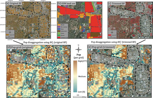
Table 4. Performance evaluation of the four weighting scenarios

Scenarios	RMSE	MAE	ORE	SE	CoE	MIoA
$B{F}_c^{\prime }$	480.96	313.53	26.24%	3.52	0.75	0.75
$B{F}_s^{\prime }$	444.43	298.74	25.55%	3.51	0.79	0.76
$B{F}_{sc}^{\prime }$	490.06	320.38	26.44%	3.54	0.74	0.75
UNIF	1102.57	606.75	52.08%	37.96	−0.32	0.58

Note. The best performance for each individual assessment metric is highlighted in bold.

4.2. Relationships between building footprints and ACS population

Linear correlation analysis was conducted to shed light on the state-level relationships between building footprint statistics and the ACS population. At a state level, all three building statistics are significantly correlated with population regardless of the trimming process (Figure 3a-3b). The strong correlation (Pearson’s r) reveals the validity of utilizing building footprints for population disaggregation. The statewide correlation between population and building count remains almost the same in both figures before and after trimming. In census survey units, however, the effectiveness of building footprint trimming should be recognized (as demonstrated in Figure 2).

Figure 3. The state-level correlation analysis: population and building count (a); population and building size (b); and the correlation between the two building statistics (c)

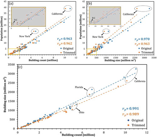
In Figure 3a-3b, New York state (NY), California (CA), and DC are highlighted using dashed ellipses as they are far away from the regression lines. These phenomena can be explained by their much higher urbanization levels than other states. High-rise apartments are common in these big cities. Their population distributions cannot be sufficiently summarized using two-dimensional building statistics (size and count), which leads to the underestimation of the population, thus resulting in their outlying positions above the regression lines in both original and trimmed cases in the two figures. Additional vertical dimension is necessary in highly urbanized areas in order to take building holding capacity (volume) into consideration (discussed in Section 5.2).

The ratio of building size and building count defines the average size of the individual buildings (AVE) in a census tract. Figure 3c indicates a strong positive correlation between building size and building count. The slope of the regression line, or the AVE, has an obvious drop after the trimming process. As shown in Figure 3a-3b, California has the highest population, building size, and count among all states. It shows the largest disparity in size and count and an apparent AVE drop after trimming (Figure 3c). Similar features are also observed in other states such as Florida that are intensely urbanized. Although not marked in the figure, the individual building size of DC drops from 433.5 $m^2$ to 295.5 $m^2$. Ohio is an example state with both AVE values (before and after trimming) below the regression lines, indicating its smaller individual building size than more urbanized states. Nevertheless, all states reveal apparent AVE drop after trimming, which proves the effectiveness of removing non-residential buildings in this study. Therefore, we only used the trimmed building footprints for the following process.

4.3. Performance of different weighting scenarios

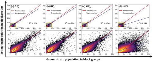
The population grids disaggregated with different weighting scenarios ($B{F}_s^{\prime }$, $B{F}_c^{\prime },B{F}_{sc}^{\prime }$ and UNIF) were evaluated at the block group level. Figure 4 presents the scatter plots for all 266,330 block groups within the CONUS. In general, population disaggregation using the three scenarios of building footprint statistics after trimming (Figure 4a-c) tends to have a much higher coefficient of determination with $R^2$(in a range of 0.761–0.794) than UNIF ($R^2$ = 0.344), indicating that building footprint statistics are relevant to population distribution at the finer unit level. Notable disagreement was observed in the UNIF scenario where population was assumed uniformly distributed within each census tract (Figure 4d). The poor performance of the UNIF scenario proved the ubiquitous existence of heterogeneity within a rather small geographic unit. Among the three building footprint scenarios, $B{F}_s^{\prime }$ (building size) has the highest $R^2$ ($R^2=0.794$), followed by and $B{F}_{sc}^{\prime }$ (building size*count) and $B{F}_c^{\prime }$ (building count).

Figure 4. Performances of the four weighting scenarios in CONUS evaluated at the block group level. (a) building count; (b) building size; (c) building size*count; (d) uniform distribution in census tracts. Only trimmed building footprints are used in a-c

The six assessment metrics for all weighting scenarios are presented in Table 4. Similarly, the building footprint-weighted population disaggregation is apparently superior to the UNIF method. For example, the ORE values for three building footprint scenarios are all lower than 30% while that for UNIF reaches 52.08%. Across the CONUS, all three footprint weighting scenarios achieve RMSE < 500 (persons) while the uniform assumption leads to RMSE > 1000 (persons). Better performance can also be found in other statistics (Table 4). Ranging from minus infinity to 1, CoE of all footprint scenarios is above 0.7, proving a better agreement of estimated population and ground-truth population. The CoE of −0.32 for the UNIF scenario confirmed that, even at a small geographic level like census tract, uniform distribution should not be assumed.

Agreeing with Figure 4, $B{F}_s^{\prime }$ achieves the best performances in all assessment metrics. It is reasonable that building size transcends building count by incorporating additional information on building holding capacity. Despite the lack of vertical dimension, the attribute of two-dimensional building size proved superior in partitioning population to each grid cell. Therefore, we adopted the building size scenario to extract the final population grid product of this study.

4.4. Disaggregating population using $\mathit{B}{F}_s^{\prime }$

Figure 5 presents the extracted 100 m population grid in the CONUS. This raster layer is about 2.5Gb in size containing approximately 800 million grid cells. The value in each cell represents the disaggregated population ranging from 0 to 9847. The product is currently hosted by ESRI (http://arcg.is/19S4qK) for visualization. Overall, the distribution of population follows the urban patterns in the CONUS, with dense population in urban and sparse population in rural areas. Population deserts, or cell clusters with extremely low population, can also be found in the Mountain States. Eight example sites in big cities of Seattle, San Jose, Los Angeles, Houston, Orlando, Miami, Atlanta, and New York City are presented in Figure 5. The exhibited heterogeneity of population within those urban fabrics primarily comes from the varying land-use patterns. With the removal of non-residential buildings tagged by OSM, it is obvious that some areas with a dense concentration of buildings are actually population deserts.

Figure 5. The 100 m population grid extracted using the $B{F}_s^{\prime }$ scenario.

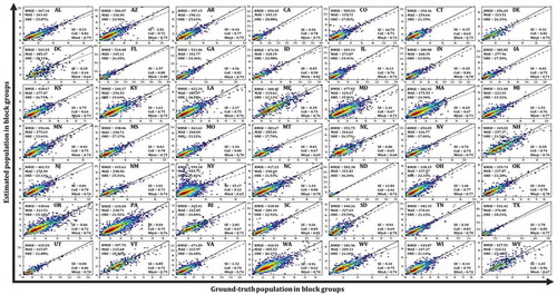
Statistics for all CONUS states are summarized in Figure 6. In general, the population grid well captured the heterogeneity of population distribution at the block group level. Forty-five out of 49 states (including DC) have ORE<30%. Vermont (VT), Wisconsin (WI), and Tennessee (TN) are the top three states with the lowest ORE values (20.95%, 21.14%, and 21.25%, respectively) while North Dakota (ND), Maryland (MD), and New York (NY) with the highest OREs (36.32%, 35.91%, and 31.81%, respectively). For CoE and MIoA, larger values represent better performance with 1.0 indicating a perfect agreement. Among the 49 CONUS states (including DC), the CoE of 37 states and MIoA of 44 states are beyond 0.7, suggesting good model performance.

Figure 6. Scatter plot heatmap of the ground-truth population against the estimated population in block groups for 49 states (DC included) of the CONUS (dashed line represents regression line, and solid line represents the 1:1 reference line)

To assess the spatial dynamics of model performance, the six accuracy assessment metrics were mapped at the state level using four-category quantile, with blue indicating good performance and red indicating bad performance (Figure 7). Overall the estimated population grids show an increased agreement from the west to east of the CONUS. The Southeast region has the best results especially with the CoE (Figure 7e) and MIoA (Figure 6f) metrics. Exceptionally, GA and FL in the Southeast are in the worst quantile in the RMSE (Figure 7a) and MAE (Figure 7b). This could be partly explained by their larger average population per block group compared with other states (GA: 1,845 and FL: 1,777), resulting in higher absolute discrepancies given their mediocre OREs (Figure 7c). In this case, CoE and MIoA reduced the outlier effects and provided a better assessment.

Figure 7. Six accuracy assessment metrics in the CONUS at the state level. RMSE (a); MAE (b); ORE (c); SE (d); CoE (e); and MIoA (f)

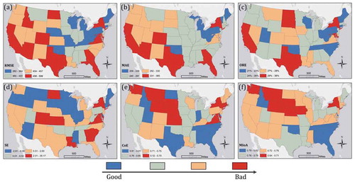
Noticeably, all six metrics for NY fall in the worst quantile. Its bad performance is presumably due to the existence of megacity of New York City (NYC). The NYC has the highest population density among all major cities in the United States (NYC Planning, 2020). Upon the ACS data of 2013–2017, its population density reaches 9,516 people per square kilometer (24,647 per square mile). High-rise dwelling units are popular, especially in urban areas. The Microsoft building footprint dataset, however, lacks a vertical dimension (building height). Therefore, population grid cells in urban areas could be underestimated while other areas in the same census tract are overestimated, resulting in higher uncertainty within the city. The NYC boundary is within five counties. Table 5 compares the six metrics between the NYC and the NY state. Averaged in five counties, the NYC always has higher RMSE, MAE, ORE, and SE, and lower CoE and MIoA than the statewide metrics, indicating worse performance within the city. The New York County where Manhattan is located has the worst performance.

Table 5. Comparison of model performance between NYC and NY state. The metric values of the state and NYC (averaged in five counties) are highlighted in bold

Counties	# of BG*	RMSE	MAE	ORE	SE	COE	MIOA
NYC
Bronx	1,154	848.30	553.72	62.67%	37.95	−0.46	0.50
Kings	2,062	599.41	423.14	40.45%	22.18	−0.17	0.54
New York	1,167	1397.79	981.97	68.62%	138.05	−3.14	0.36
Queens	1,739	515.68	353.79	30.80%	5.17	0.36	0.64
Richmond	324	442.54	308.71	24.93%	−2.41	0.63	0.72
Averages above	/	760.74	524.27	45.49%	40.19	−0.55	0.55
NY State	15,405	599.18	345.71	31.81%	35.17	0.12	0.65

*BG represents the block group.

5. Discussion

5.1. Uncertainties in trimming building footprints

This study used the crowdsourced OSM land-use dataset to eliminate non-residential buildings. Its large spatial coverage, detailed tagging of land-use types, and frequent updates (daily) make OSM a great source for this purpose. The trimming process effectively enhanced the spatial heterogeneity of population distribution, especially within complicated urban fabrics. Table 6 shows a comparison of population disaggregating results between the weighting scenario using original building footprint size ($B{F}_s$) and weighting scenario using trimmed building footprint size ($B{F}_s^{\prime }$). Each metric in the table is an average of all states in the CONUS. Again, the statistical result proves the improvement of the trimming process as $B{F}_s^{\prime }$outperforms $B{F}_s$ in RMSE, MAE, ORE, CoE, and MIoA.

Table 6. Before and after building footprint trimming

Scenarios	RMSE	MAE	ORE	SE	CoE	MIoA
$B{F}_s$ (original)	462.40	316.27	27.74%	1.27	0.77	0.75
$B{F}_s^{\prime }$ (trimmed)	444.43	298.74	25.55%	3.51	0.79	0.76

Despite the improvement in assessment statistics, its intrinsic limitations should not be overlooked. Due to the nonprofessional, voluntary public participation of the OSM project, concerns regarding the data quality have been raised. Estima and Painho (2013) explored the classification accuracy of the OSM land-use dataset in Continental Portugal and reported a global accuracy around 76%. Arsanjani, Mooney, Zipf, and Schauss (2015) reported an overall accuracy of 87% in Berlin, 90.6% in Frankfurt, 88.9% in Hamburg, and 86.2% in Munich. To our best knowledge, the quality of the OSM landuse dataset has not been thoroughly evaluated in the CONUS. The wrong tags (misclassification) and inaccurate boundaries of OSM land-use polygons might propagate uncertainties towards the final population grid. Another limitation is the incompleteness of OSM product. As reported by Haklay (2010), OSM data tend to be more complete in urban than in rural areas and in developed countries than in developing countries. This inevitably creates spatial biases across space. In this study, the incompleteness of OSM land-use data results in partial removal of non-residential buildings, thus leading to the wrong partition of population into land-use types such as commercial, grocery, industrial, and institutional lands.

Nevertheless, it needs to be stated that the OSM is a long-term project and is updating its dataset on a daily basis. New efforts have also been made to collect open-sourced map data all over the globe. For example, the Humanitarian OpenStreetMap Team (HOT), is an international team to create open map data in support of global humanitarian action such as disaster management (www.hotosm.org). The POPGRID Data Collaborative (www.popgrid.org), established in 2020, expands the international community of data providers, users, and stakeholders to share high-quality data grids on population, human settlements, and infrastructure. With more land-use classes updated in the future, it will be able to play a more trustful role in extracting and updating population grids.

5.2. Intrinsic problems of microsoft building footprints

While Microsoft building footprints have proved a promising source for population disaggregation, cautions should be advised for future studies as the data itself exhibited intrinsic problems as observed in this study.

5.2.1. Data deficiencies

Several notable deficiencies in Microsoft building footprints have been observed. Despite that this dataset is the most current and comprehensive building footprints dataset in the CONUS, the problem of its incomprehensiveness still exists. Occasionally in a densely populated urban area, there exist some strips of missing buildings. Clusters of missing buildings in a certain block group potentially result in the underestimation of population in this unit and therefore the overestimation in other units within the same census tract (the disaggregation method preserves the total population in each tract).

Additionally, Microsoft footprint dataset contains a large number of small-size polygons that are not buildings. Visual interpretation on Google Earth imagery shows that those small-size polygons often represent false detections including garages, trailers, temporal awnings, etc. In this study, a 50 $m^2$ threshold was empirically selected and proved effective in eliminating most of them. The threshold, however, is subjective and may not remove all of these small-size nonresidential polygons.

The building footprint product sometimes mistakenly merged multiple buildings to one polygon, particularly in densely urbanized areas where individual buildings lie close to each other. In this case, the population grid disaggregated using building footprint size is less affected than using building footprint count. It may explain why footprint size slightly outperforms footprint count in the disaggregation process as shown in this study (Table 4). Finally, some shape distortions and location displacements have been noted in both rural and urban areas, although they are not substantial in determining population distribution.

5.2.2. Lack of vertical dimension of buildings

The Microsoft building footprints do not contain any building height information. The lack of vertical dimension of buildings introduces great uncertainty in estimating building holding capacity, causing significant population underestimation for highly urbanized areas with high-rise buildings. Even though the OSM data removed a majority of high-rise commercial use buildings in urban areas, the existence of high-rise mixed-use and residential buildings gives a great challenge in population estimation when building vertical information is missing. In this study, the underestimation of population has been observed for many block groups in large cities that predominantly contain high-rise condominiums, holding unexpectedly larger population than their building footprint size has reflected. To better disaggregate population in cities, building height information should be considered in the future analysis.

5.2.3. Temporal uncertainty

Released in June 2018, the Microsoft building footprint dataset is the most up-to-date open-source building footprints in the CONUS. However, its vintage depends on the underlying Bing Imagery, which is a composite of multiple imaging sources in various temporal periods. It is difficult to know the exact dates for individual pieces of data (Microsoft, 2019). Despite its full geographic coverage over the CONUS, the temporal uncertainty in the dataset might cause problems for studies that require certain temporal restrictions. Although the change of buildings is slow in developed countries like the US, the mismatch in building footprints resulting from data latency still hampers the extracted population grids in terms of timeliness. With the advance of deep learning algorithms and the emergence of commercialized high-resolution images, this dataset could be gradually updated with improved quality.

5.3. Future directions

Given the limitations aforementioned, future work is needed to provide better population grid products with improved spatial and temporal explicit. For example, analysis could be done to incorporate an additional dimension of buildings (height). Studies have been conducted to extract the vertical dimension of buildings from LiDAR and aerial photogrammetry (Stal, Tack, De Maeyer, De Wulf, & Goossens, 2013). The building height information contributes to a better estimation of building volume, significantly improving population estimation for densely populated urban areas.

In light of numerous limitations of the OSM land-use dataset, a better strategy for categorizing building usage is needed. Attempts have been made to generate better land-use map via Earth observations (Yang, Fu, Smith, & Yu, 2017), auxiliary government databases (Theobald, 2014) and mobile phones (Pei et al., 2014). Although the robustness of those products and proposed methods awaits further exploration, they offer new ways to identify buildings that are likely to be residential, thus contributing to improved trimming process of building footprints.

Besides building footprints in this study, other sources of weighting variables could be explored in population disaggregation. However, cautions need to be advised when coarse-resolution (e.g. sub-km level) variables are incorporated. The lack of heterogeneity at this level possibly introduces more uncertainties, thus undermining the accuracy of the derived population grid. Here, we recommend two high spatially explicit layers that can be potentially incorporated to improve the population grid. Launched in June 2017 by China, the Luojia 1–01 satellite complements the existing nighttime light data with a high spatial resolution of 130 m (Jiang et al., 2018), significantly improving the 5 km DMSP-OLS (Defense Meteorological Program Operational Line-Scan System) and 742 m VIIRS (Visible Infrared Imaging Radiometer Suite) imagery. Given the high correlation between light intensity and population density, the improved artificial light observation with such high spatial resolution renders a new aspect to model population distribution and therefore can be integrated with building footprints. Transportation network has proved strongly relevant to population distribution. Given the completeness of opensource road network data provided by the US Census Bureau, its derivatives (e.g., road density and distance to the road) could be a valuable indicator of population distribution at a national scale.

Finally, future work is needed on updating those building footprints for a temporal continuation of the high-resolution population grid. The emergence of very high-resolution imagery from commercial satellites and SmallSat systems largely facilitates this process. Imagery captured by Quick Bird (60 cm), GeoEye-1 (50 cm), WorldView-1 (50 cm), WorldView-2 (46 cm), and WorldView-3 (31 cm) provides sufficient details for building footprint detection using well-trained deep learning models. Assisted by the advance of computation capabilities (e.g., the improvement of Graphics Processing Unit) and detecting algorithms, updating existing building footprints within a fixed temporal period becomes possible. Derived from constantly updated building footprints, the high spatial- and temporal-resolution population grids can greatly contribute to a variety of studies including public health, disaster assessment, humanitarian relief operations, and planning.

6. Conclusion

This study explores the feasibility and best practices of utilizing the open-source Microsoft building footprints to disaggregate the ACS census surveyed population (2013–2017) and presents a 100 m population grid in the CONUS. The crowdsourced OSM land-use data was used to trim the non-residential areas out of the building footprints. The building size was found in the most suitable weighting scenario in a dasymetric method because it provides optimal information of building holding capacity. The increased heterogeneity after footprint trimming led to improved population distribution, especially within complicated urban fabrics. Overall, the population grids in the US Southeast reached the best agreement although the six metrics had varying performance in different states, especially in states with the megacities such as New York. The results suggest that building footprints alone can summarize the heterogeneity of population at the census unit level and therefore, provides better population estimates with higher spatial details across the CONUS.

This study earns valuable experience in integrating census survey and open-source satellite-based building footprints and crowdsourced land uses to create high-resolution population grid in a large geographic context. Our product can benefit a wide range of studies that require spatially explicit population data. It is currently hosted by ESRI (http://arcg.is/19S4qK) for visualization and can be accessed via for visualization and can be accessed via https://doi.org/10.7910/DVN/DLGP7Y. Future work will focus on incorporating the vertical dimension of buildings, designing a better building categorization strategy, and integrating other data sources of weighting layers. With the exploding evolution of Big Earth Data, the approach tested in this study and the preliminary population grid product could be easily updated and improved for both spatial and temporal continuation on the globe.

Disclosure statement

No potential conflict of interest was reported by the authors.

Data availability statement

The product can be visualized at http://arcg.is/19S4qK. To download the data, please visit https://doi.org/10.7910/DVN/DLGP7Y.

References

- ACS, When to Use 1-year, 3-year, or 5-year Estimates. (2018). https://www.census.gov/programs-surveys/acs/guidance/estimates.html
- Ahola, T., Virrantaus, K., Krisp, J. M., & Hunter, G. J. (2007). A spatio‐temporal population model to support risk assessment and damage analysis for decision‐making. International Journal of Geographical Information Science, 21(8), 935–953.
- Arsanjani, J. J., Mooney, P., Zipf, A., & Schauss, A. (2015). Quality assessment of the contributed land use information from OpenStreetMap versus authoritative datasets. In J. J. Arsanjani, A. Zips, P. Mooney & M. Helbich (Eds.), OpenStreetMap in GIScience (pp. 37–58). Cham: Springer.
- Azar, D., Engstrom, R., Graesser, J., & Comenetz, J. (2013). Generation of fine-scale population layers using multi-resolution satellite imagery and geospatial data. Remote Sensing of Environment, 130, 219–232.
- Balk, D., Deichmann, U., Yetman, G., Pozzi, F., Hay, S. I., & Nelson, A. (2006). Determining global population distribution: Methods, applications and data. Advances in parasitology, 62, 119–156.
- Chai, T., & Draxler, R. R. (2014). Root mean square error (RMSE) or mean absolute error (MAE)?–Arguments against avoiding RMSE in the literature. Geoscientific Model Development, 7(3), 1247–1250.
- Dmowska, A., & Stepinkski, T. F. (2017). A high resolution population grid for the conterminous United States: The 2010 edition. Computers, Environment and Urban Systems, 61, 13–23.
- Dobson, J. E., Bright, E. A., Coleman, P. R., Durfee, R. C., & Worley, B. A. (2000). LandScan: A global population database for estimating populations at risk. Photogrammetric Engineering and Remote Sensing, 66(7), 849–857.
- Doxsey-Whitfield, E., MacManus, K., Adamo, S. B., Pistolesi, L., Squires, J., Borkovska, O., & Baptista, S. R. (2015). Taking advantage of the improved availability of census data: A first look at the gridded population of the world, version 4. Papers in Applied Geography, 1(3), 226–234.
- Eicher, C. L., & Brewer, C. A. (2001). Dasymetric mapping and aerial interpolation: Implementation and evaluation. Cartography and Geographic Information Science, 28(2), 125–128.
- Estima, J., & Painho, M. (2013). Exploratory analysis of OpenStreetMap for land use classification. In Proceedings of the Second ACM SIGSPATIAL International Workshop on Crowdsourced and Volunteered Geographic Information (Vol. 1, pp. 39–46). November 5, 2013.
- Fonte, C., Minghini, M., Patriarca, J., Antoniou, V., See, L., & Skopeliti, A. (2017). Generating up-to-date and detailed land use and land cover maps using OpenStreetMap and GlobeLand30. ISPRS International Journal of Geo-Information, 6(4), 125.
- Fotheringham, A. S., & Wong, D. W. (1991). The modifiable areal unit problem in multivariate statistical analysis. Environment & Planning A, 23(7), 1025–1044.
- Freire, S., & Pesaresi, M. (2015). GHS population grid, derived from GPW4, multitemporal (1975, 1990, 2000, 2015). European Commission, Joint Research Centre (JRC). PID: http://data. europa.eu/89h/jrcghsl-ghs_pop_gpw4_globe_r2015a
- Frye, C., Wright, D. J., Nordstrand, E., Terborgh, C., & Foust, J. (2018). Using classified and unclassified land cover data to estimate the footprint of human settlement. Data Science Journal, 17(20), 1–12.
- Guo. (2017). Big earth data: A new frontier in Earth and information sciences. Big Earth Data, 1(1–2), 4–20.
- Haklay, M. (2010). How good is volunteered geographical information? A comparative study of OpenStreetMap and Ordnance Survey datasets. Environment and Planning. B, Planning & Design, 37(4), 682–703.
- Homer, C. G., Dewitz, J. A., Yang, L., Jin, S., Danielson, P., Xian, G., … Megown, K. (2011). Completion of the 2011 National Land Cover Database for the conterminous United States—Representing a decade of land cover change information. Photogrammetric Engineering and Remote Sensing, 81(5), 345–354.
- Jiang, W., He, G., Long, T., Guo, H., Yin, R., Leng, W., … Wang, G. (2018). Potentiality of using Luojia 1-01 nighttime light imagery to investigate artificial light pollution. Sensors, 18(9), 2900.
- Klein Goldewijk, K., Beusen, A., Van Drecht, G., & De Vos, M. (2011). The HYDE 3.1 spatially explicit database of human‐induced global land‐use change over the past 12,000 years. Global Ecology and Biogeography, 20(1), 73–86.
- Leyk, S., Gaughan, A. E., Adamo, S. B., de Sherbinin, A., Balk, D., Freire, S., … Pesaresi, M. (2019). The spatial allocation of population: A review of large-scale gridded population data products and their fitness for use. Earth Syst. Sci. Data, 11(3), 1385–1409.
- Li, X., & Zhou, W. (2018). Dasymetric mapping of urban population in China based on radiance corrected DMSP-OLS nighttime light and land cover data. Science of the Total Environment, 643, 1248–1256.
- Linard, C., Alegana, V. A., Noor, A. M., Snow, R. W., & Tatem, A. J. (2010). A high resolution spatial population database of Somalia for disease risk mapping. International Journal of Health Geographics, 9(1), 45.
- Lu, J., Carbone, G. J., & Gao, P. (2017). Detrending crop yield data for spatial visualization of drought impacts in the United States, 1895–2014. Agricultural and Forest Meteorology, 237, 196–208.
- Microsoft. (2019). Microsoft/USBuildingFootprints. March 04 https://github.com/Microsoft/USBuildingFootprints
- Murdock, A. P., Harfoot, A. J. P., Martin, D., Cockings, S., & Hill, C. (2015). OpenPopGrid: An open gridded population dataset for England and Wales. GeoData, University of Southampton. http://openpopgrid.geodata.soton.ac.uk/
- Nadim, F., Kjekstad, O., Peduzzi, P., Herold, C., & Jaedicke, C. (2006). Global landslide and avalanche hotspots. Landslides, 3(2), 159–173.
- Nash, J. E., & Sutcliffe, J. V. (1970). River flow forecasting through conceptual models part I—A discussion of principles. Journal of Hydrology, 10(3), 282–290.
- NYC Planning (2020). Population – New York City population. accessed March 27, 2020. Department of City Planning, New York City. https://www1.nyc.gov/site/planning/planning-level/nyc-population/population-facts.page
- Palacios-Lopez, D., Bachofer, F., Esch, T., & Heldens, W. (2019). New perspectives for mapping global population distribution using world settlement footprint products. Sustainability, 11(21), 6056.
- Pei, T., Sobolevsky, S., Ratti, C., Shaw, S. L., Li, T., & Zhou, C. (2014). A new insight into land use classification based on aggregated mobile phone data. International Journal of Geographical Information Science, 28(9), 1988–2007.
- Ramm, F., Names, I., Files, S. S., Catalogue, F., Features, P., Features, N., & Cars, C. (2014). OpenStreetMap data in layered GIS format. Version, 6, 7.
- Reed, F. J., Gaughan, A. E., Stevens, F. R., & Yetman, G. (2018). Gridded population maps informed by different built settlement products. Data, 3(3), 33.
- Small, C., & Nicholls, R. J. (2003). A global analysis of human settlement in coastal zones. Journal of Coastal Research, 19(3), 584–599.
- Smith, S. K., Nogle, J., & Cody, S. (2002). A regression approach to estimating the average number of persons per household. Demography, 39(4), 697–712.
- Stal, C., Tack, F., De Maeyer, P., De Wulf, A., & Goossens, R. (2013). Airborne photogrammetry and lidar for DSM extraction and 3D change detection over an urban area–a comparative study. International Journal of Remote Sensing, 34(4), 1087–1110.
- Tatem, A. (2017). WorldPop, open data for spatial demography. Sci Data, 4(1), 2017.
- Theobald, D. M. (2014). Development and applications of a comprehensive land use classification and map for the US. PloS One, 9(4), e94628.
- Tiecke, T. G., Liu, X., Zhang, A., Gros, A., Li, N., Yetman, G., … Dang, H. A. H. (2017). Mapping the world population one building at a time. arXiv, 1712, 05839.
- Wardrop, N. A., Jochem, W. C., Bird, T. J., Chamberlain, H. R., Clarke, D., Kerr, D., … Tatem, A. J. (2018). Spatially disaggregated population estimates in the absence of national population and housing census data. Proceedings of the National Academy of Sciences, 115(14), 3529–3537.
- Willmott, C. J., Ackleson, S. G., Davis, R. E., Feddema, J. J., Klink, K. M., Legates, D. R., … Rowe, C. M. (1985). Statistics for the evaluation and comparison of models. Journal of Geophysical Research: Oceans, 90(C5), 8995–9005.
- Yang, D., Fu, C. S., Smith, A. C., & Yu, Q. (2017). Open land-use map: A regional land-use mapping strategy for incorporating OpenStreetMap with earth observations. Geo-spatial Information Science, 20(3), 269–281.
- Yuan, J. (2018). Learning building extraction in aerial scenes with convolutional networks. IEEE Transactions on Pattern Analysis and Machine Intelligence, 40(11), 2793–2798.