Understanding satellite images: a data mining module for Sentinel images

ABSTRACT

The increased number of free and open Sentinel satellite images has led to new applications of these data. Among them is the systematic classification of land cover/use types based on patterns of settlements or agriculture recorded by these images, in particular, the identification and quantification of their temporal changes. In this paper, we will present guidelines and practical examples of how to obtain rapid and reliable image patch labelling results and their validation based on data mining techniques for detecting these temporal changes, and presenting these as classification maps and/or statistical analytics. This represents a new systematic validation approach for semantic image content verification. We will focus on a number of different scenarios proposed by the user community using Sentinel data. From a large number of potential use cases, we selected three main cases, namely forest monitoring, flood monitoring, and macro-economics/urban monitoring.

KEYWORDS:

• Data mining
• Earth observation
• Sentinel-1
• Sentinel-2
• image semantics
• classification maps
• analytics
• third party mission data

1. Introduction

The Copernicus Access Platform Intermediate Layers Small Scale Demonstrator (CANDELA) project is a European Horizon 2020 research and innovation project for easy interactive analysis of satellite images on a web platform. Among its objectives are the development of efficient data retrieval and image mining methods augmented with machine learning techniques as well as interoperability capabilities in order to fully benefit from the available assets, the creation of additional value, and subsequently economic growth and development in the European member states (Candela, 2019).

The potential target groups of users of the CANDELA platform are: space industries and data professionals, data scientists, end users (e.g., governmental and local authorities), and researchers in the areas covered by the project use cases (e.g., urban expansion and agriculture, forest and vineyard monitoring, and assessment of natural disasters) (Candela, 2019).

When it comes to image analysis and interpretation, the main objectives of our application-oriented data mining CANDELA platform can be grouped into five activities (Candela, 2019):

• Activity 1: A Big Data analytics building block allowing the analysis of large volumes of Earth observation (EO) data.

In our case, this activity will generate a large geographical and temporal volume of EO data to be ingested into the data analytics building blocks.

• Activity 2: Tools for the fusion of various multi-sensor Earth observation satellite data (comprising, besides Sentinel, also several other contributing missions) with in-situ data and additional information from the web such as social networks or Open Data, in order to pave the way for new applications and services.

Our achievements will be measured by the capability to ingest data from various and heterogeneous sources (EO data and non-EO data).

• Activity 3: Compatibility of the analytics building blocks with any cloud computing back-office layers in order to run our applications on a distributed architecture with complete scalability and elasticity, and eventually to be deployed on top of our Sentinel data interface (DIAS) (2020).

  Our goal is the compatibility between the CANDELA platform, other existing European assets, and future DIAS developments.

• Activity 4: Analytics tools developed for the platform that will have state-of-the-art performance, and allow us to obtain optimal veracity.

This can be verified by checking the attainable accuracy of our results.

• Activity 5: Development of realistic reference scenarios that demonstrate the platform capabilities and use cases, and their functionality to new external users.

This can be checked by validation of the given use cases.

The focus of this paper is the definition of real scenarios/use cases (cf. Activity 5) using as much Earth observation data as possible being available for each use case (cf. Activity 1). Our project uses the data provided by Sentinel-1 and Sentinel-2.

Until the date of the submission of this paper [June 2020], the Copernicus Sentinels generated more than 27 million Earth observation (EO) products. More than 300,000 users have downloaded this Big EO data. Due to their high spatial resolution, Sentinel-1 and Sentinel-2 data represent ca. 90% of the total Copernicus EO data volume. The data are free and the access is open. Systems as the European Space Agency (ESA) Copernicus Open Access Hub (Candela, 2019; Sentinel-1, 2019), the Thematic Exploitation Platforms (TEPs) (Thematic Exploitation Platforms, 2020) or the Copernicus Data and Information Access Services (DIAS) (DIAS platform, 2020) provide access to the data.

The very recent Machine Learning advent as a general-purpose methodology is presently converting the entire landscape of technology in any field. In this context, we based the Data Mining component in CANDELA on Active Machine Learning for EO, in a hybrid paradigm with parameter estimation, information retrieval, and specific aspects of EO image semantics, including elements of ontology focused on Sentinel-1 and Sentinel-2 observations. The Data Mining is changing the “data access” into “information and knowledge” extraction. The fast and adaptive operation of the Data Mining component is one of the assets to increase the valorisation of the Sentinel-1 and Sentinel-2 data and broadening their application areas.

The paper is organized as follows: Section 2 presents the proposed use cases, and the targeted data together with their characteristics. Section 3 explains the scientific background of our approach, and the CANDELA platform. Typical validation results are presented in Section 4, followed by some conclusions, and future work in Section 5.

2. Presentation of the use cases

In this section, we start by explaining the characteristics of the data set, and by introducing the selected use cases.

2.1. Characteristics of sentinel data

The Sentinel-1 mission comprises a constellation of two satellites (called A and B), operating in C-band for synthetic aperture radar (SAR) imaging. Sentinel-1A has been launched on April 1st, 2014, while Sentinel-1B has been launched two years later on April 25th, 2016 (Sentinel-1, 2019). The repeat period of each Sentinel-1 satellite is 12 days, which means that every 6 days, there may be an image acquisition of the same site by one of the two satellites. As SAR has the advantage of operating at wavelengths not impeded by thin cloud cover or a lack of solar illumination, one can acquire data over large areas during day or night time with almost no restrictions due to weather conditions.

From the multitude of product options that exist, we selected Level-1 Ground Range Detected (GRD) products with high resolution (HR) taken routinely in Interferometric Wide swath (IW) mode (Sentinel-1, 2019). These data are produced (prior to geo-coding) with a pixel spacing of 10 × 10 m and correspond to about 5 looks and a resolution (range × azimuth) of 20 × 22 m. For these products, the data are provided in dual polarization, namely VV and VH in WGS 84 geometry. For rapid and efficient high-resolution feature extraction with a good signal-to-noise ratio, we simply used the VV polarization data.

In contrast, the Sentinel-2 mission also comprises a constellation of two satellites (also called A and B), but collects multispectral (optical) data being affected by the actual weather conditions (e.g., cloud cover). The Sentinel-2A satellite has been launched on June 23rd, 2015, while Sentinel-2B has been launched on March 7th, 2017 (Sentinel-2, 2019). Both Sentinel-2 instruments have 13 spectral channels (in the visible/near infrared, and in the short wave infrared spectral range). The repeat period of each Sentinel-2 satellite is 10 days. That means every 5 days there can be an image acquisition of the same site by one of the two satellites.

In this case, we selected Level-1 C products which were radiometrically and geometrically corrected WGS 84 images with ortho-rectification and spatial registration on a global reference system with sub-pixel accuracy (Sentinel-2, 2019). For visualization, the RGB bands of Sentinel-2 (B04, B03, and B02) were used to generate quick-look quadrant images. For feature extraction, the user can choose different band combinations. In this paper, we selected the four high-resolution 10 m bands of Sentinel-2 mages with man-made infrastructures content and all 13 bands (at 10 m, 20 m and 60 m) for Sentinel-2 images with natural vegetation content. This selection was made based on our experience/validation and the observations seen during the analysis of Sentinel-2 data.

This selection of Sentinel products mostly will result in a larger number of semantic labels for Sentinel-2 data, in contrast with Sentinel-1 data. This is due to the higher resolution of the Sentinel-2 and the capability to identify more classes from the image content.

2.2. Selected use cases

Based on different European user workshops, we selected half a dozen use cases for Sentinel images. The presented use cases in this paper are grouped in three main categories and are linked to Activity 5 of the project. Each category is divided into sub-categories in order to demonstrate the complexity of the problem and the diversity of cases that we may encounter. These use cases are: monitoring of forests (fires, windstorms and deforestation), monitoring of floods (river, sea, and ocean), and monitoring of urban areas.

For each use case (see Table 1), the user communities provided us with objectives and their requirements, consolidated solution approaches, and typical image examples.

Table 1. Selected use cases and their parameters

Use case	Objectives	Image criteria	Processing steps		Selected images	Validation
Forest Monitoring	Burnt forest areas	Comparison of pre- and post-event images		Target area selection Classification Labelling Comp. of percentages	Amazon Rainforest Sentinel-1 Sentinel-2	Comparison with other publications
	Windstorm effects	Comparison of pre- and post-event images		Target area selection Classification Labelling Comp. of percentages	National Park in Poland Sentinel-1 Sentinel-2	Done by the user community
	Deforestation	Comparison of pre- and post-event images		Target area selection Classification Labelling Comp. of percentages	Romania Sentinel-1	International NGO and local press reports
Flood monitoring	River floods	Comparison of pre- and post-event images		Target area selection Classification Labelling Comparison of percentages	Mississippi River in Nebraska Sentinel-2	Local press reports
	Ocean floods	Post-event image		Classification Labelling	Mozambique coastline Sentinel-1 Sentinel-2	Single press report
Urban monitoring	Discernible urban categories	Single images		Target area selection Classification Labelling	One image per continent Sentinel-1 Sentinel-2	Google Earth, hackathon, and other publications

2.2.1. Forest monitoring

The objective of the forest use case aims to present how Earth observation satellite data collection can be used for the monitoring of the forests in different conditions such as fires, windstorms, deforestations, etc.

2.2.1.1. Fires in the Amazon rainforest area

In August 2019, many fires affected the Amazon rainforest. Based on a report by the European Space Agency (ESA), the numbers of fires were four times higher than in the year 2018. The fires that occurred together with some (legal or illegal) deforestation left the land for future agricultural use but may result in rising global temperatures (ESA: Fires ravage the Amazon, 2019).

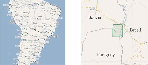
In this use case, we focused on the area between Brazil, Bolivia, and Paraguay. For the fire period in August 2019, we were able to acquire both Sentinel-1 and Sentinel-2 satellite images. As for Sentinel-1, the selected images were acquired on August 2nd, August 26th, and September 7th, 2019, while for Sentinel-2, the selected images were acquired on August 5th, August 20th, August 25th, and September 9th, 2019.

The location of the affected area is shown in Figure 1.

Figure 1. Location of our Amazonian target area marked on Google Maps (Google Maps, 2019)

2.2.1.2. Windstorms in Poland

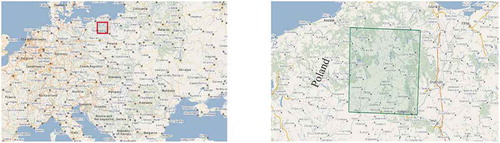
In mid-August 2017, a large area of forest near the Bory Tucholskie National Park in Poland was affected by windthrow. The location of the affected area is outlined in Figure 2.

Initially, the park was created in July of 1996 and now covers an area of 46 km² of forests, lakes, meadows, and peatlands. The park is located in the northern part of Poland in the heart of the Tuchola Forest, the largest woodland in Poland. In 2010, this park was included in the UNESCO Tuchola Forest Biosphere Reserve.

Also for this area, both Sentinel-1 and Sentinel-2 images were available during several intervals that could be used for investigation. Based on the available data, we selected Sentinel-1 images that were acquired (prior to the windstorm) on July 30th, 2017, and (after the windstorm) on August 29th, 2017, while the Sentinel-2 images were acquired (prior to the windstorm) on July 30th, 2017, and (after the windstorm) on September 28th, 2017.

Figure 2. Location of our target area in Poland marked on Google Maps (Google Maps, 2019)

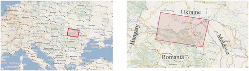
2.2.1.3. Deforestation in Romania

From 2005 to 2009, more than 1,000 hectares of forest around Tarnita Balasanii were illegally decimated, although the whole area is a fully protected area of the Maramures Natural Park Mountains. In 2016, 220 hectares of forest were cut in this area. As a consequence, a number of natural disasters took place (e.g., landslides and floods), and many houses and agricultural crops were destroyed.

For this area, only Sentinel-1 images were available. Thus, we chose an image taken on June 27th, 2015 before the deforestation, and an image acquired on September 1st, 2016 after the deforestation was discovered.

The location of the deforested area is shown in Figure 3.

Figure 3. Location of our target area in Romania marked on Google Maps (Google Maps, 2019)

2.2.2. Flood monitoring

The objective of the second use case aims to show the use of the Earth observation satellite data for monitoring the area affected by floods and how this is evolving over the time.

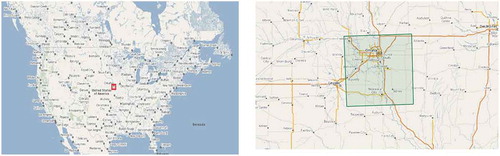
2.2.2.1. Floods in Omaha, Nebraska

In March 2019, floods occurred in and around the city of Omaha, Nebraska (United States of America) near the Missouri river. A large area of the city and of its surroundings were affected by the floods.

From the available Sentinel images, we only selected some multispectral Sentinel-2 images as they provide the only complete coverage of the affected area. These products were acquired as a pre-disaster image, an image recorded during the floods, and a post-disaster image.

Due to the required cloud-free imaging, the selected pre-disaster image had already been acquired on March 1st, 2018. The image during the floods was acquired on March 21st, 2019. Due to the spring season, the image has a different appearance than the post-disaster image taken some weeks later. This image was acquired on June 24th, 2019, and represents a summer image.

The location of the affected area is depicted in Figure 4.

Figure 4. Location of our target area in Nebraska marked on Google Maps (Google Maps, 2019)

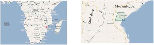
2.2.2.2. Floods in Beira, Mozambique

In March 2019, another flooding took place in the same period with the one from Omaha, but this time in Beira, Mozambique caused by the Cyclone Idai.

The selection of Sentinel data was more difficult in this case. In the case of Sentinel-1, we were only able to find a single image acquired on March 19th, 2019 that covers the entire area of the flooding. As for Sentinel-2, the only available image was acquired on March 22nd, 2019; however, the image is covered by clouds and could not be used for land cover classification.

The extent of the flooded area is shown in Figure 5.

Figure 5. Our target area in Mozambique marked on Google Maps (Google Maps, 2019)

2.2.3. Macro-economics

The objective of the “macro-economics” use case is to show how remote sensing capacities to extract adequate information from urban images which will be used to feed economical models.

2.2.3.1. Monitoring of urban areas over the world

We selected a number of cities and their surrounding areas from different countries, with different architectures, and recorded by Sentinel-1 and/or Sentinel-2.

This use case demonstrates the impact of the definition and selection of semantic categories for different geographical locations and architectures of the cities combined with the influence of the type of instrument being used for the image acquisition. The cities were grouped per continent and by imaging technique. The list of the selected cities is further detailed together with their locations marked in Figure 6.

Figure 6. Locations of the selected cities marked on Google Maps (Google Maps, 2019)

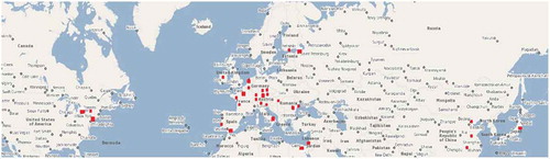
• Asia: Beijing (Sentinel-2), Haikou (Sentinel-2), Shanghai (Sentinel-2), Tokyo (Sentinel-1 and Sentinel-2), Wuhan (Sentinel-2);

• Europe: Amsterdam (Sentinel-1 and Sentinel-2), Bari (Sentinel-1), Bordeaux (Sentinel-2), Bratislava (Sentinel-2), Brussels (Sentinel-2), Budapest (Sentinel-2), Dublin (Sentinel-2), Huevel (Sentinel-2), Lisalmi (Sentinel-2), Lisboa (Sentinel-1), Milan (Sentinel-2), Munich (Sentinel-1), Paris (Sentinel-2), Prague (Sentinel-2), Saint Petersburg (Sentinel-2), Santarem (Sentinel-2), Setubal (Sentinel-2), Tampere (Sentinel-2), Toulouse (Sentinel-2), Vienna (Sentinel-2), Venice (Sentinel-1), and Zurich (Sentinel-2);

• Middle East: Tel Aviv (Sentinel-1) and Cairo (Sentinel-2);

• North America: New York (Sentinel-2) and Toronto (Sentinel-1).

3. Description of the CANDELA Platform

CANDELA’s main objective is the creation of additional value from Sentinel images through the provisioning of modelling and analytics tools assuming that the tasks of data collection, processing, storage, and access will be carried out by the Copernicus Data and Information Access Service (DIAS) (DIAS platform, 2020). After the integration of all components, CANDELA will be deployed on top of CreoDIAS (CreoDIAS, 2019). CreoDIAS is an environment that brings the algorithms to the EO data. This platform contains online almost all the Sentinel satellite data (Sentinel-1, Sentinel-2, Sentinel-3, and Sentinel-5P), and other EO data (e.g., Landsat-5, Landsat-7, Landsat-8, and Envisat).

The CANDELA platform allows the prototyping of EO applications by applying efficient data retrieval and data mining tools augmented with machine learning techniques as well as the interoperability among Sentinel-1 and Sentinel-2 in order to fully benefit from their potential content-related data, and thus, to add more value to the satellite data. It also helps us to interactively detect many objects or structures, and to classify land cover categories (Candela, 2019).

The design, implementation or operation of high-complexity systems require an analysis from different perspectives. For CANDELA, we proposed View Model, which is a standardized engineering system (e.g., IEEE Standard 1471–2000). This model has three perspectives (see Figure 7):

• Information Processing: dealing with the basic information content transformation by algorithms, and their use and interoperation;

• Software Architecture: performing the computational and functional decomposition of the system architecture;

• Operations to be Performed: monitoring the sequences of operations and running the use cases.

3.1. Information processing

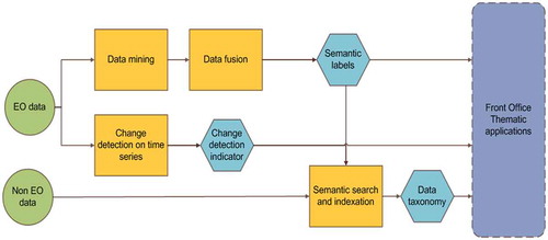
In CANDELA, the EO data are analyzed by two processing chains (see the data flow in Figure 8): by “Data Mining” together with “Data Fusion”, and by “Change Detection”.

The Data Mining and Data Fusion module extracts textual content descriptors (i.e., “semantic land cover labels” (Dumitru, Schwarz, & Datcu, 2016)) in the actual EO product, whereas Change Detection extracts information for “change indicators” to be provided to the users (see “Thematic Applications” in Figure 8).

Some non-EO data (e.g., cadastral maps, weather parameters) can be objects of search and semantic indexing that, if necessary, can be combined with EO data semantics. The resulting data taxonomy is transferred to use case-dependent Thematic Applications (e.g., outlines of affected areas).

In this paper, we focus only on the EO Data Mining assets, and how to add more value to the satellite data. It also helps interactively detect objects or structures, and to classify land cover categories, while the design, implementation or operation of high-complexity systems require an analysis from different perspectives.

The other modules presented in Figure 8 (except Data Mining), namely Data Fusion, Change Detection, and Semantic Search and indexation are described in (Candela, 2019) and separately in Datcu, Dumitru, & Yao (2019b). (Aubrun et al., 2020), and Dorne et al. (2020).

Figure 7. The View Model of CANDELA seen from three perspectives

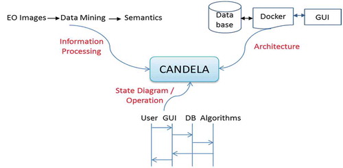
Figure 8. Block diagram of the CANDELA platform modules as information processing flow (Candela, 2019)

3.2. Software architecture

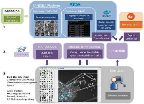
The Data Mining batch processing software is integrated with the CANDELA system containers and Dockers (Datcu, Dumitru, & Yao, 2019a) (see Figure 9). An interface assures the transfer of the EO products (e.g., Sentinel-1 and Sentinel-2 data) from CreoDIAS (CreoDIAS, 2019).

In the Data Model Generation-Data Mining (DMG-DM) container, the data model generation processes for data mining are run for each selected product. After the completion of DMG-DM, the extracted metadata and features are ingested into the Database Management System (DBMS) database on the platform that can be used for querying product metadata, features, and semantic labels (Datcu et al., 2019a). The information is available on the platform and can be downloaded by local users via a Representational State Transfer (RESTful) service (REST API, 2019).

The users, accessing the GUI interface, have to perform numerical classifications (i.e., feature grouping) via active learning methods. Later, during an annotation step, these classification results can be converted into semantic labels (sometimes called categories).

The annotated semantics (Dumitru, Schwarz, & Datcu, 2018; Dumitru et al., 2016) are ingested via Internet into the remote database on the platform.

3.3. Operations to be performed

The EO standard (i.e., pre-processed) products are decomposed into features and metadata within the Data Model Generation (DMG) module. Then, the extracted actionable information and metadata are ingested into the database management system (via a MonetDB database (MonetDB, 2019)).

Figure 9. Architecture of the Data Mining module on the platform and front end (Datcu et al., 2019a)

The DMG module transforms the original format of the original EO products into smaller and more compact product representations that include features, metadata, image patches, etc. The database management system module is used for storing all the generated information, and allows for querying and retrieval within the available feature and metadata space. In contrast, the Data Mining module is in charge of finding user-defined patterns of interest via machine learning algorithms within the processed data and presenting the results to the users for final semantic annotation. The proper selection of the appropriate semantic annotation (label/category) for a patch is based on the majority of the content of the selected patch (burnt forest areas, flooded areas, etc.).

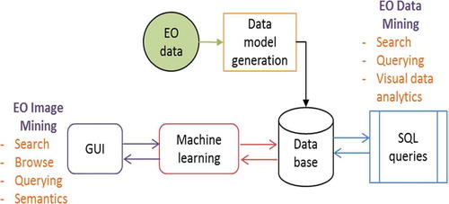
Data Mining (see the general overview in Figure 10) is operated in two modes: EO Image Mining and EO Data Mining. The outputs of Data Mining are common semantic maps.

Figure 10. Data Mining functions, components, and interfaces

• EO Image Mining: Here, the users run a machine learning tool/component via its interactive GUI (in Figure 11) based on an Active Learning module (Blanchart, Ferecatu, Cui, & Datcu, 2014) (in a form of supervised machine learning) which is using all actionable information. The learning algorithm is able to interactively interrogate a user (information source) to label new data points with the desired outputs.

The key idea behind Active Learning is that a machine learning algorithm can achieve greater accuracy with fewer training examples if it is allowed to choose the data from which it learns. The input is the training data sets obtained interactively from the GUI. The training dataset refers to a list of images marked as positive or negative examples. The output is the verification of the Active Learning loop sent to the GUI and the semantic annotation written in the DBMS catalogue.

In conclusion, the functions are search, browse, and query for image patches of interest to the user. The discovered relevant structures are semantically annotated and stored into the DBMS. The tool uses only image features. The results of the actual EO image semantics are learned and adapted to the user conjectures and applications.

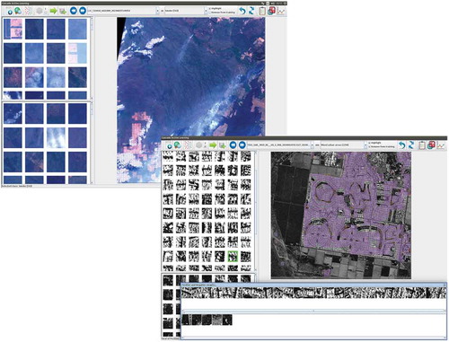
Figure 11. GUI interface of Image Mining (Top): Interactive interface to retrieve images belonging to the categories that exist in a collection (e.g., Smoke). The upper left half shows relevant retrieved patches, while the lower left half shows irrelevant retrieved patches. The large GUI panel on the right shows the image that is being worked on, and which can be zoomed. (Bottom): The same interactive interface, but in this case, the users can verify the selected training samples by checking their surroundings as there is a link between the patches in the upper left half and the right half. Here, the magenta color on the big quick-look panel shows the retrieved patches being similar to the ones provided by the user. The user can also see the selected patches selected by him/her as relevant and irrelevant patches (bottom part of the GUI)

Active Learning methods include Relevance Feedback which supports users to search images of interest in a large repository. The GUI allows automatically ranking the suggested images, which are expected to be grouped in the class of relevance. Visually supported ranking allows enhancing the quality of search results by giving positive and negative examples.

During the Active Learning two goals are achieved: 1) learn the targeted image category as accurately and as exhaustively as possible and 2) minimize the number of iterations in the relevance feedback loop.

Active Learning has important advantages when compared with Shallow Machine Learning or Deep Learning methods, as presented in Table 2.

Table 2. Comparison between Shallow machine learning (ML), Deep Learning, and Active Learning

	Shallow ML	Deep Learning	Active Learning
Training data volume	Medium (GB)	Very high (PB)	Very small (0.1 KB)
Trained data volume	Large (GB-TB)	Very high (PB)	Large (GB-TB)
No. of classes	up to 100	up to 100	Any user defined
Classification accuracy	Avg. 85%	Avg. 90%	Avg. 85%
Training speed	Medium (hours)	Slow (days)	Fast (minutes)

Particularly for the EO image application Active Learning with very small training samples makes possible their detailed verification; thus, the results are trustable, avoiding the plague of training database biases. Another important asset is its adaptability to the user conjecture. The EO image semantics is very different from other definitions in geoscience, as cartography for example. The EO image is capturing the actual reality on ground, and the user can discover and understand it freely, extracting the best meaning, thus enriching the EO semantic catalogue.

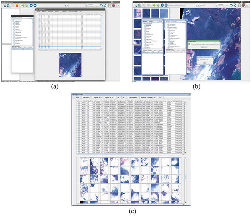
Figure 12. (a) Query interface of Data Mining. (Left:) Select the query parameters, e.g., “metadata_id”, “mission”, and “sensor” and enter the desired query values in the query-expression table below. (Right:) Display the products that match with the query criteria (“mission” = S2) including their metadata and image files. (b) Query interface of Data Mining. (Left:) Select the metadata parameters (e.g., “mission = S2A” and “metadata_id = 39”) and (Right) semantics parameters (e.g., “name = Smoke”). Depending on the EO user needs, it is possible to use only one or to combine these two queries. The combined query is returning the number of results from the database (in this case 543). (c) Query interface of Data Mining. This figure presents a list of images matching the query criteria (from Figure 12b). The upper part of the figure shows a table composed of several metadata columns corresponding to the patch information while the lower part of the figure presents a list of the quick-looks of patches that corresponds to the query

• EO Data Mining: This is performed via SQL searches (see Figure 12(a-c)), queries, and browsing extracting the data analytics information. Data Mining uses image features, image semantics, and selected EO product metadata.

The state diagram of the user operations is depicted in Figure 13 and comprises the following sequence of steps:

Figure 13. Operation state diagram of Data Mining

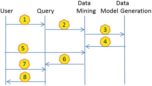
(1) Identify the imaging instrument: Here, the user decides which Sentinel products shall be selected.

(2) Identify the Sentinel products and transfer them to Data Mining: Choose the area to be processed via the CreoDIAS platform.

(3) Process the Sentinel products in Data Model Generation: Use the DMG module in order to extract the metadata and select the algorithm appropriate to the Sentinel data for feature and descriptor extraction. Select also the number of grids/levels.

(4) Extract the descriptors and transfer them to Data Mining: Compute the features and ingest the results into the database for further use.

(5) Run the Image Mining function: Users can search and mine for selected content based on their requirements.

(6) Extract Sentinel semantics: Ingest the semantically annotated content (i.e., the labelled patches) into the database. The used taxonomy for annotation is like a list of labels from which the user can choose or define some.

(7) Query and combine the Sentinel semantics with the metadata: The user can now run queries based on metadata of the Sentinel products, based on the semantics (annotated by the user or available via the database) or by combing both query types.

(8) Generate analytics results: The output of the results will be in the form of statistical results, semantic classification maps, etc.

4. Performance testing and validation of the use cases via the CANDELA Platform

4.1. Testbed approach

We assume that we can rely on high-quality validation data. Therefore, when we use the CANDELA web platform, after the selection of the data for each use case, the images are processed directly by Data Model Generation and are ready for the Data Mining module.

Each Sentinel image is cut into patches with a pre-selected size depending on the actual image ground sampling distance in order to cover an area of about 200 × 200 m on the ground. Based on the characteristics of the data, we selected for Sentinel-1 a patch size of 128 × 128 pixels, while for Sentinel-2 the patch size was 120 × 120 pixels (EOLib project, 2019).

The Active Learning in the Data Mining module is also powered with our spatial multigrid strategy. The EO image patches are partitioned in a pyramid, e.g., at a first scale in a 120 × 120 pixel grid, at a second finer scale in 60 × 60 pixel grid and in third even finer grid, a 30 × 30 pixel grid (in the case of Sentinel-2). As for Sentinel-1, the grids are 128 × 128 pixels, 64 × 64 pixels, and 32 × 32 pixels.

The Active Learning has a mechanism to hierarchically make semantic annotations, from coarse to fine grids. The mechanism is supported by a statistical decision, which discards not relevant patches when going to a finer grid. This is a specific Big Data solution. It is possible to enlarge the labelled data by up to three orders of magnitude using a very small training data set, typical 10s of samples.

For example in (Datcu et al., 2020), for the “Water bodies” category, we are using about 12% from the entire amount of patches (at the first grid/level), while the rest of the patches are assigned to other categories and discarded from the classification. These patches are split again (in the second grid), classified, and the residues that do not belong to the desired category are removed (we keep 65% of all patches). On the third grid/level, we repeated this procedure and we were finally annotating 94% of the patches with the category we are looking for.

The quick-look views of the patches are stored in a database for further use via the GUI of the Data Mining module (Dumitru et al., 2016).

The extracted features describing each original patch can then be extracted. The available libraries of algorithms implemented in the platform are Gabor filters with linear moments or logarithmic cumulants (MPEG7, 2019), Weber local descriptors (Chen et al., 2010), and multispectral histograms (Georgescu, Vaduva, Raducanu, & Datcu, 2016). The experiments show that for SAR images the best feature extraction method is Gabor Linear Moments (e.g., with five scales and six orientations) (MPEG7, 2019) for man-made infrastructure categories (e.g., Urban and Industrial areas, Transportation), while for natural categories (e.g., Agriculture, Forest, Natural vegetation) the Adaptive Weber Local Descriptor is the best performer (e.g., with 8 orientations and 18 excitation levels) (Chen et al., 2010). A comparison between different feature extraction methods is already described in (Dumitru & Datcu, 2013) for high-resolution TerraSAR-X images. For multi-spectral images, the best feature extraction method is the Weber Local Descriptor (e.g., with 8 orientations and 18 excitation levels) (Georgescu et al., 2016). The extracted features of each patch are then stored in our database.

These features are then routinely classified (i.e., in an unsupervised approach) using Data Mining and grouped into clusters using machine learning based on Cascaded Active Learning (Blanchart et al., 2014). In our case, we used a Support Vector Machine (SVM) classifier with a χ² kernel and a one-against-all approach.

This proposed approach is implementing also a second important function, the hierarchic labelling of the EO images (Dumitru et al., 2016). Firstly, the multi-grids generate a finer localization of the semantic class, this is a quad-tree like spatial-multiscale structure. Secondly, since semantic is changing with scale of the image patches, a semantic tree is generated. This is an explainable method, i.e., an image patch at the coarsest scale is indexed with more detailed meaning at finer scales.

The entire information is stored into the database and can be further queried or can be used to generate additional analytics (e.g., semantic classification maps, statistical analytics, etc.).

Some statistics of the volume of data analysed using the Data Mining module and their diversity of locations is presented in Table 3. This table is showing the volume of the data analysed using the CANDELA platform (more precisely, the Data Mining module). From the available data, we selected the appropriate one for our use cases. The semantic labels were selected from (Dumitru et al., 2016) and represent individual labels (if the same label appears several times, in will be marked only once).

Table 3. The amount of data processed by the Data Mining module

Sensor type		Sentinel-1	Sentinel-2
Number of processed images		35	137
Locations	Asia	6	10
	Europe	14	122
	Middle East	4	5
	North America	5	15
	South America	3	7
	North Pole	3	0
Average image size (pixels)		26,400 × 16,600	10,980 × 10,980
Surface covered in km^2		400,000	175,000
Number of bands		1 band	3 bands: 45 4 bands: 74 13 bands: 18
Patch size (pixels)		128 × 128	120 × 120
Number of patches		2, 074, 377	9, 630, 818
Number of annotated patches		399, 040	266, 270
Number of semantic “individual” labels		44	61

4.2. Experimental results

In this paper, we illustrate the usefulness of the platform by six examples, outline the classification results, and demonstrate different statistics obtained from the data. For all use cases, we exploited appropriate image data. For ease of use, we kept the same color coding for each semantic category/label. Any remaining differences between the labelling results can be due to the actual resolution and the patch size of the data.

4.2.1. Forest monitoring results

4.2.1.1. Experimental results for the fires in the Amazon rainforest use case

For this use case, we selected a multi-sensor and multi-temporal data set, acquired by Sentinel-2 and Sentinel-1. Based on the availability of both instruments, we were able to select more than 10 images for each instrument for a period from beginning of August to the beginning of September 2019. As the highest intensity of the fires occurred around August 25th, 2019, we aimed at obtaining images acquired before, during, and after the fire.

Using the Data Mining module, we were able to classify and to semantically annotate all selected images, and to extract several analytics from which we could then extract other statistics. The resulting quick-look views of the investigated areas together with their semantic classification maps are depicted in Figure 14 for Sentinel-1 data, and in Figure 15 for Sentinel-2 data.

From these two figures, we can see that the difference in resolution between the instruments also has an implication for the number of extracted categories.

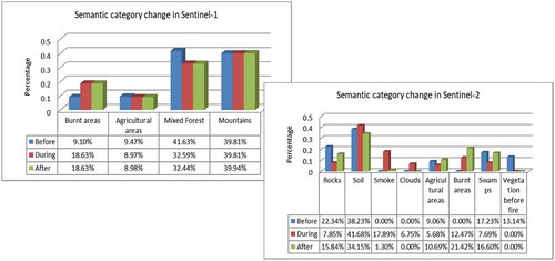
Figure 16 shows the diversity of the discernible categories, and the changes between the three acquisition dates using Sentinel-1 data (left-hand side of the figure), and Sentinel-2 data (right-hand side of the figure).

In the case of Sentinel-2, by counting the number of patches semantically annotated as Burnt areas, we can easily compute the affected area. Knowing the resolution of 10 m (using the Sentinel-2 bands B2, B3, and B4 with a resolution of 10 m), and a patch size of 120 × 120 pixels, we obtain an area of 12 km² for the image acquired during the fire on August 25th, 2019, and an area of 23 km² for the image acquired after the fire expired on September 9th, 2019.

Similar results are obtained using the Sentinel-1 data. The largest area affected by fires is a Mixed forest area, and very small percentages are Agricultural areas. We can see that the Burnt areas double between August 2nd and August 25th, 2019. From the same figure, we can observe how some categories, that had a larger area before the event, are reduced or categories with smaller area are increased, and even new categories appeared (e.g., Burnt areas).

Figure 14. A multi-temporal data set for the first use case. (From left to right and from top to bottom): Quick-look views of the first Sentinel-1 image from August 2nd, 2019, of the second image from August 26th, 2019, and of the last image from September 7th, 2019, followed by the classification map of each of the three images

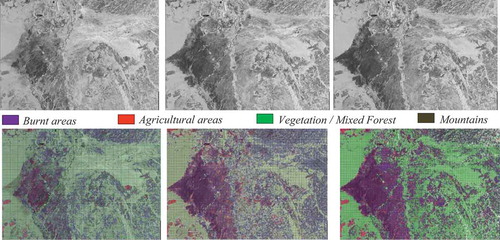
Figure 15. A multi-temporal data set for the first use case. (From left to right and from top to bottom): An RGB quick-look view of a first Sentinel-2 image from August 5th, 2019, of the second image from August 25th, 2019, and of the last image from September 9th, 2019, followed by the classification maps of each of the three images

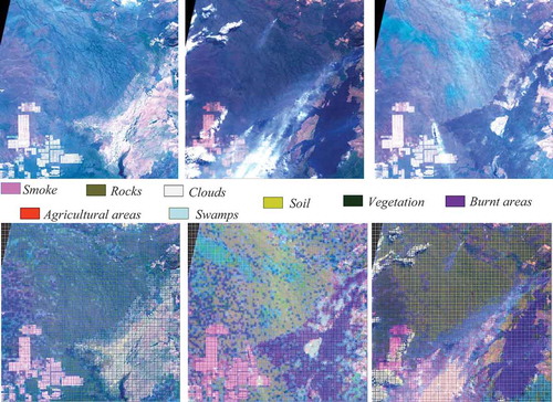
Figure 16. Diversity of categories, and the change of categories identified from three Sentinel-1 images (top) and three Sentinel-2 images (bottom) that cover the area of interest of the first use case. The Sentinel-1 images were acquired on August 2nd, 2019, August 26th, 2019, and on September 7th, 2019, while the Sentinel-2 images were acquired on August 5th, 2019, August 25th, 2019, and on September 9th, 2019

4.2.1.2. Experimental results for the windstorms in Poland use case

For this use case, we selected a multi-sensor and multi-temporal data set, acquired by Sentinel-1 and Sentinel-2 (see Figures 17 and 18). This helps evaluate the area affected by the windstorms. In both cases, the first image was acquired on July 30th, 2017, as the pre-event image, while the second image is the post-event image.

Figure 17. A multi-sensor and a multi-temporal data set for the second use case. (Top – from left to right): A quick-look view of a first Sentinel-2 image from July 30th, 2017, and its classification map, and a quick-look view of a second Sentinel-2 image from September 28th, 2017, and its classification map. (Bottom – from left to right): A quick-look view of a first Sentinel-1 image from July 30th, 2017, and its classification map, and a quick-look view of a second Sentinel-1 image from August 29th, 2017, and its classification map

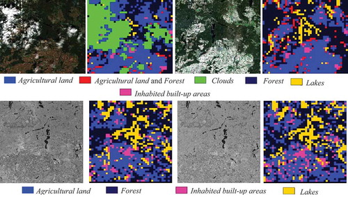
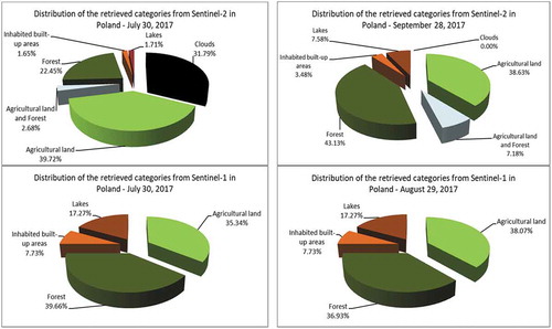
Figure 18. Diversity of categories identified from two Sentinel-2 and two Sentinel-1 images that cover the area of interest of the second use case. (From left to right and from top to bottom): The distribution of the retrieved and annotated categories of the Sentinel-2 images acquired on July 30th, 2017 and on September 28th, 2017, and the categories of the Sentinel-1 images acquired on July 30th, 2017 and on August 29th, 2017. The differences between the Sentinel-2 and Sentinel-1 results can be explained by clouds being only visible in Sentinel-2 images. For the different labels, see Section 4.2

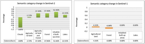
Due to the cloud coverage compromising the Sentinel-2 images, it is difficult to evaluate the affected forest area, but by analyzing the Sentinel-1 data of the same area on the ground, we were able to compute the area in km² simply based on the percentage of the amount of Forest now appearing and annotated as Agriculture areas (we do not have a Wind-damage label category).

From Figure 19, we can extract the percentage of the affected area. Knowing the patch size of the Sentinel-1 data of 128 × 128 pixels together with the given pixel spacing and resolution, we could compute the affected forest area as 42 km².

Figure 19. Semantic label changes between two Sentinel-1 images (right) and two Sentinel-2 images (left) acquired for the second use case. The value of the changes should be multiplied by 100 in order to obtain the percentage of the change. The results are given for the windstorms in Poland

4.2.1.3. Experimental results for the deforestation in Romania use case

For this use case, only very few Sentinel-1 images were available. From them, we chose an image recorded in 2015 as a pre-event image to be sure that no big deforestation had already taken place, and we selected another image after the deforestation had been discovered (as a post-event image). See the results shown in Figures 20 and 21.

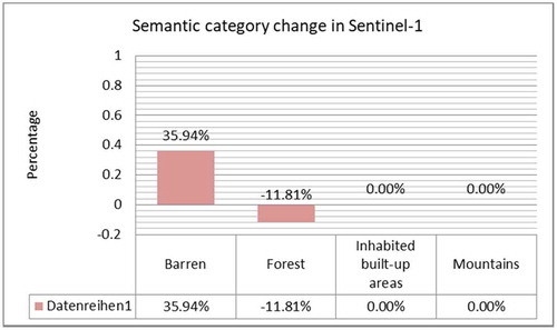
After the classification, we were able to generate Figure 22, from which we can see that the percentage of deforestation amounts to 12%. Knowing the patch size of the Sentinel-1 data of 128 × 128 pixels together with their given pixel spacing and resolution, we computed the deforested area as comprising 46 km².

Figure 20. A multi-temporal data set for the fifth use case (From left to right, first two columns): A quick-look view of a first Sentinel-1 image from June 27th, 2015, and its classification map. (From left to right, last two columns): A quick-look view of a second Sentinel-1 image from September 1st, 2016, and its classification map

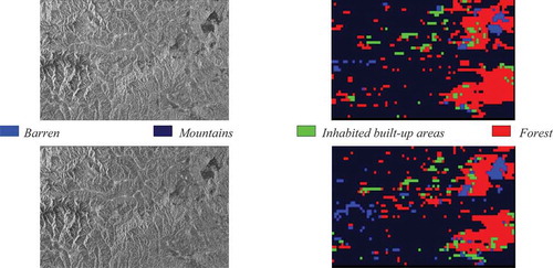
Figure 21. Diversity of categories identified from two Sentinel-1 images that cover the area of interest of the fifth use case. (From left to right): Distribution of the retrieved and annotated categories of the images acquired on June 27th, 2015, and on September 1st, 2016

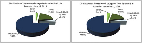
Figure 22. Semantic label changes between two Sentinel-1 images acquired for the fifth use case

4.2.2. Flood monitoring results

4.2.2.1. Experimental results for the floods in the Omaha use case

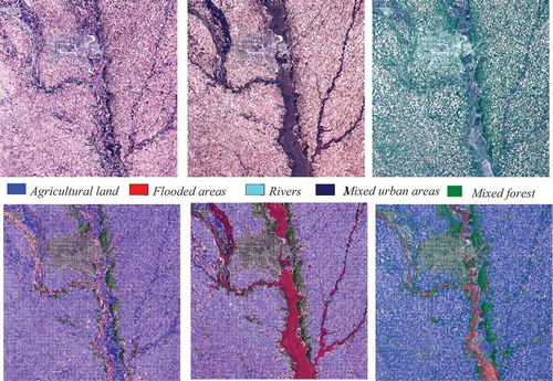
For this use case, three images were selected as a pre-event image, an image taken during the flooding, and a post-event image. Each image was processed using the platform tools, and each patch of the images was semantically annotated using the hierarchical annotation scheme described in (Dumitru et al., 2016). From the content of these images, we were able to extract five semantic categories, namely Agricultural land (which includes prairies and grasslands), Mixed forest, Rivers, Mixed urban areas, and Flooded areas (a category that appears in the second and third images).

The results of the annotation are shown in Figure 23, where each image is shown as an RGB quick-look image (bands B4, B3, and B2 at 10 m resolution of Sentinel-2), alongside the classification map generated after the annotation.

Figure 23. A multi-temporal data set for the third use case. (From left to right and from top to bottom): An RGB quick-look view of a first Sentinel-2 image from March 1st, 2018, of the second image from March 21st, 2018; and the last image from June 24th, 2018, followed by the classification maps of each of the three images

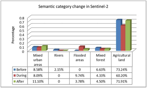
By querying the database for each semantic category, we were able to generate some statistical analytics. An example is Figure 24, from which we can see the changes that appear among the three images.

In Figure 24, it can be seen that, after the floods, the category Mixed urban areas increased unnaturally much across the images. This occurred due to the visibility of buildings within the scenes when the annotation was made. One explanation can be that some buildings were not visible and were included in Agricultural land. Because, during the period when the first two images were taken, it was winter, and the area was covered by snow, compared to the last image that was taken in summer.

Another category for which we noticed changes is Rivers. This category appears only in the pre-event image, because then this category is merged with a new one, namely Flooded areas. This category is found during the event, and in the post-event image.

Extracting the percentage of the Flooded areas from Figure 24, and knowing the patch size for the classification of 120 × 120 pixels, and the resolution of 10 m of the Sentinel-2 image, we can compute the affected area in km² for the event image, and the post-event image. For the event image, the affected area covers about 1000 km², which shrank, after three months, to 445 km².

Figure 24. Distribution of retrieved semantic categories for the three images of the third use case, the floods in Omaha, Nebraska, USA

4.2.2.2. Experimental results for the floods in the Beira use case

In this use case, we initially tried to retrieve images from Sentinel-1 (2019) and Sentinel-2 (2019) that cover the area of interest (like in use case 3), but these images were not available or were affected by clouds (see Figure 25 bottom-left). Finally, an image of Sentinel-1 was available after the floods. We chose also one image of Sentinel-2 in order to demonstrate the influence of the clouds.

Both images were semantically annotated and we retrieved the following categories: Sea, Small vessels, Brush/Rangeland, Mixed urban areas, Mountains, Clouds, and Flooded areas.

In the case of Sentinel-1, which is not affected by clouds, we were able to classify the area affected by the floods. An evaluation of the annotated Sentinel-2 image brought us to the conclusion that only a small area of the flooded surface was visible through the clouds. The results of both classifications are presented in Figure 25.

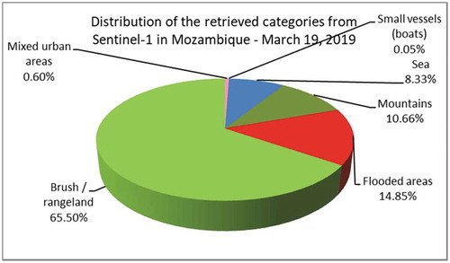
The distribution of the retrieved and classified categories is illustrated in Figure 26 (only for the Sentinel-1 data).

When considering the percentage obtained after classification for the category of Flooded areas and knowing the patch size of the Sentinel-1 data (e.g., 128 × 128 pixels), their resolution of 20 m, and the pixel spacing of 10 m, we could compute the affected areas. In this case, the total affected area was 330 km².

Figure 25. A multi-sensor data set for the fourth use case (Top -from left to right): A quick-look view of a Sentinel-1 image from March 19th, 2019, and its classification map. (Bottom -from left to right): An RGB quick-look view of a first Sentinel-2 image from March 22nd, 2019, and its classification map

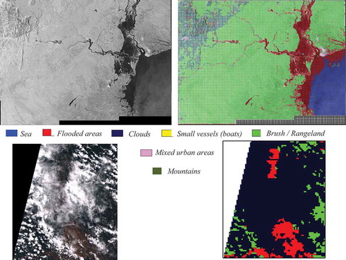
Figure 26. Diversity of categories identified from a Sentinel-1 image that covers the area of interest of the fourth use case

4.2.3. Urban monitoring results

4.2.3.1. Experimental results for the monitoring of urban areas use case

The results of the last use case were ordered alphabetically (first the continent, and after that the city). The full list of analyzed cities is shown in Section 2.2.6. Because of space limitations, we picked up from the full list four cities to show in this paper.

Tokyo and surrounding areas

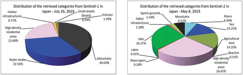
For the first city, we found an image for each instrument with close acquisition dates based on the availability and cloud-free conditions of Sentinel-2. Comparing the two classification results (see Figure 27), we noticed that for Sentinel-2 with 10 m resolution it was possible to retrieve more categories than for Sentinel-1 with 20 m resolution. The diversity of the retrieved categories and the percentage of each category are depicted in Figure 28.

Figure 27. A multi-temporal data set for Tokyo and its surrounding areas. (Top -from left to right): A quick-look view of a first Sentinel-1 image from July 26th, 2019, and its classification map. (Bottom -from left to right): A quick-look view of a second Sentinel-2 image from May 8th, 2019, and its classification map

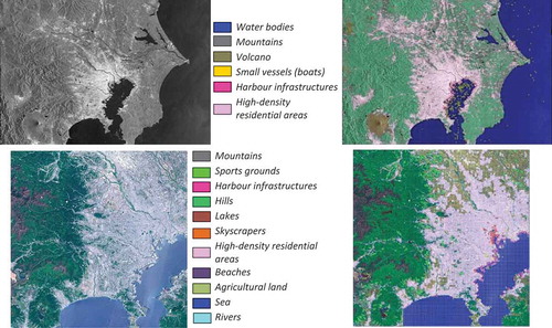
Figure 28. Diversity of categories extracted from a Sentinel-1 image and from a Sentinel-2 image that are covering the area of interest of Tokyo and its surrounding areas. (From left to right): The distribution of the retrieved and semantically annotated categories of the images acquired on July 26th, 2019, and on May 8th, 2019. The differences between Sentinel-1 and Sentinel-2 results are mainly due to the higher resolution of the Sentinel-2 data

For the category Mountains retrieved from the Sentinel-1 image, it was not possible to separate Mountains from Hills, but it was possible to separate the Volcano from the category Mountains. Also from the classification map, we can see that for Sentinel-1, it was possible to extract the category Boats because of their higher reflectance when compared to Water bodies.

Amsterdam and surrounding areas

Similar to Tokyo, we selected one image from Sentinel-1 and one image from Sentinel-2.

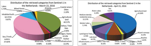
Comparing the classification results from Figure 29, once more the number of retrieved categories for Sentinel-2 is higher than the discernible categories for Sentinel-1. Using Sentinel-2, it was possible to find separately Ijssel Lake, Marker Lake, and the categories Tidal flats/Deltas that for Sentinel-1 are classified as Sea. The category Agricultural land from Sentinel-1 was split into two categories of Sentinel-2 data. The diversity of each category is shown in Figure 30.

Figure 29. A multi-temporal data set for Amsterdam and its surrounding areas. (Top -from left to right): A quick-look view of a first Sentinel-1 image from March 22nd, 2016, and its classification map. (Bottom -from left to right): An RGB quick-look view of a second Sentinel-2 image from April 21st, 2016, and its classification map

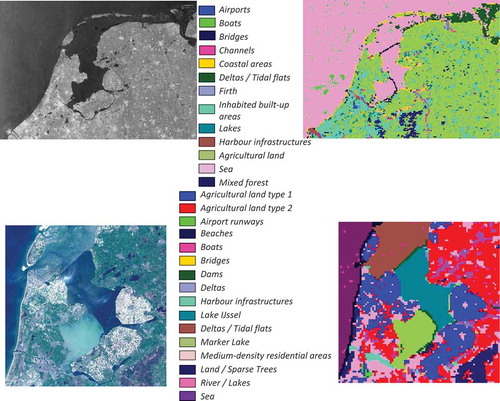
Figure 30. Diversity of categories identified from a Sentinel-1 image and from a Sentinel-2 image that are covering the area of interest of Amsterdam and its surrounding areas. (From left to right): The distribution of the retrieved and semantically annotated categories of the images acquired on March 22nd, 2016, and on April 21st, 2016. The differences between Sentinel-1 and Sentinel-2 results are mainly due to the higher resolution of the Sentinel-2 data

Saint Petersburg and surrounding areas

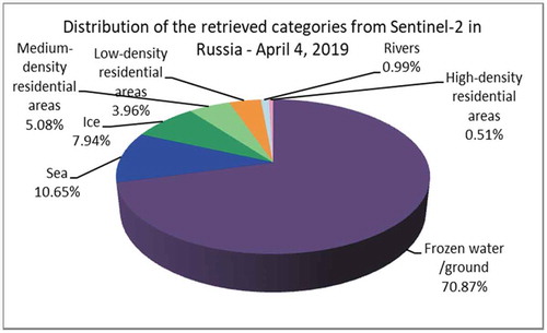
For this city, we selected a single Sentinel-2 image, as no Sentinel-1 data were available for this period. When analyzing this image, we identified an interesting category, namely Frozen water/ground (see Figures 31 and 32). When using the Sentinel-2 data, it was not possible to extract more individual categories or to split this category into other categories. However, we expect using the Sentinel-1 data to be able to separate or to split the categories Ice or Frozen water (Dumitru, Andrei, Schwarz, & Datcu, 2019).

Figure 31. A data set for Saint Petersburg and its surrounding areas. (From left to right): An RGB quick-look view of a Sentinel-2 image from April 4th, 2019, and its classification map

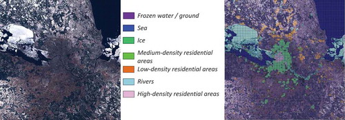
Figure 32. Diversity of categories identified from a Sentinel-2 image that is covering Saint Petersburg, Russia. This image was acquired on April 4th, 2019

Cairo and surrounding areas

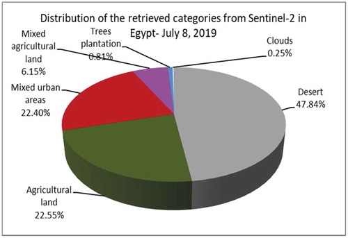
Also here, only Sentinel-2 data were available. During classification, we encountered a problem with the Desert category, which has a high reflectance, and in some areas, the image covering some other objects. The results of the classification and the diversity of the retrieved categories are demonstrated in Figures 33 and 34.

Figure 33. A data set for Cairo and its surrounding areas. (From left to right): An RGB quick-look view of a Sentinel-2 image from July 8th, 2019, and its classification map

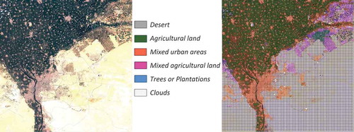
Figure 34. Diversity of categories identified from a Sentinel-2 image that is covering Cairo, Egypt. This image was acquired on July 8th, 2019

4.3. Discussions

4.3.1. Observations about the use cases

For all the use case (but especially for the urban one), we observed that the number of semantic labels retrieved for Sentinel-2 is higher than the one obtained for Sentinel-1. For example, in Figure 27, the number of semantic labels retrieved for Sentinel-2 is 11 labels, while for Sentinel-1 there are only 6 labels. This means that the sensor resolution influences the number of semantic labels that can be extracted and classified. This we observed much earlier in Dumitru et al. (2018), when we compared the high-resolution SAR images at 2.9 m resolution provided by TerraSAR-X with medium-resolution SAR images at 20 m resolution provided by Sentinel-1.

For the forest use case, if the area is not covered by clouds, we recommend to use Sentinel-2 images because they are higher resolution, can be extracted more details and can lead to a better separation between the categories (e.g., Smoke, Clouds) and sometimes these categories do not appear in Sentinel-1 (e.g., Smoke). For more details, see Figure 15 vs. Figure 14.

For the floods use case, both sensors can be used, but for a better accuracy Sentinel-1 is more appropriate. In the case of Omaha, because for that area there were no Sentinel-1 images, we used Sentinel-2 images (which were not covered by clouds) and the results are very satisfactory. In the case of Beira, the area was covered by clouds and the images from Sentinel-1 were very few. This is the reason why we could not make an assessment of the affected area without an image before or after the event.

For the urban use case, we noticed that definitions and the number of retrieved categories are influenced by the geographical location of the city and the architecture of the city (including the size of the city and the density of the city) (Dumitru, Cui, Schwarz, & Datcu, 2015). We did another study related to the simultaneous processing of several images using the Data Mining module, and we noticed that for a better grouping of categories it is necessary that the image comes from the same geographical location or has the same architecture.

4.3.2. Data mining validation

The validation of the Data Mining module prior to its integration with the CANDELA platform was made in (EOLib project, 2019), where, for the first time, a data set of multispectral images (e.g., WorldView) and a large data set of SAR images (e.g., TerraSAR-X) were classified and semantically annotated (Dumitru et al., 2018) with an accuracy of about 95%.

As part of Activity 5, during the EO Big Data Hackathon (Joint Hackathon 2019), we conducted a large-scale validation and testing of our Data Mining module. In two days, five European H2020 projects (including CANDELA) funded by the same EO-2-2017 EO Big Data Shift Call (CORDIS, 2019) were tested and evaluated by a large number of expert users in the field (including the reviewers of the European Commission (European Commission, 2019)) from the point of view of the maturity of the algorithms and the usability of the platforms.

A more detailed analysis of the Data Mining module was made within the project by two partners that had the role of users, namely SmallGIS and Terranis (see the deliverables in Candela (2019)).

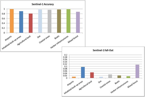
Finally, a quantitative evaluation measure of the module was performed in order to access how good the retrieved results satisfied the user’s query intent. The following metrics were used for evaluating the performance of the Data Mining module: Precision/Recall, Accuracy, F-measure, Fall-Out, Specificity, and ROC-Curve. The definition of these metrics can be found in (Manning, Raghavan, & Schütze, 2008; Powers, 2011). From this list Accuracy and Fall-Out are selected for a number of categories.

Accuracy is an alternative metric to Precision/Recall for evaluating the retrieval systems, that is, the fraction of their classifications that are correct.

Fall-Out is the proportion of non-relevant documents that are retrieved, out of all non-relevant document being available. In binary classification, this metric is closely related to Specificity and is equal to (1-Specificity).

The metric results are shown in Figure 35 for Sentinel-2 and Sentinel-1. The overall accuracy is about 93–94% for both sensors depending on the location and content of the images.

Figure 35. (a) Performance evaluation metrics for a selected number of man-made structures and natural categories retrieved from Sentinel-2 images. (b). Performance evaluation metrics for a selected number of man-made structures and natural categories retrieved from Sentinel-1

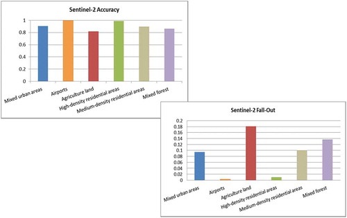
Figure 35. (Continued)

4.3.3. Comparison of CANDELA with other EO big data platforms

Four other projects similar to the CANDELA project funded by the European Commission in the frame of Big Earth observation data platforms are (H2020 EO Big Data Shift call, 2020): the BETTER project (Big data Earth observation technology and tools enhancing research and development), the EOpen project (Open source interface between Earth observation data and front-end applications), the PerceptiveSentinel project (Big data knowledge extraction and re-creation platform), and the OpenEO project (Open source interface between earth observation data and front-end applications).

Based on the discussions that we had among the projects, we noticed a number of similarities and possibilities for further cooperation with the EOpen project in the frame of Big Earth observation data and analytics. The comparison between the two projects is made from the point of the information retrieval module of the two platforms. The similarities and differences are:

• Input data: Both are processing Sentinel-2 data, but the Data Mining module is processing also Sentinel-1 and other satellite missions. Both are using 120 × 120 pixels for Sentinel-2.

• Extracted features: The component of EOpen is using deep learning features, while the Data Mining module is using standard classification features.

• Supervised/unsupervised learning: The component of EOpen is unsupervised, while the Data Mining module based on active learning is a supervised/semi-supervised learning tool.

• Semantic classes: The component of EOpen is dealing with specific classes such as Water, Snow, Rice, Forest, Vineyards, Rock, and Urban (similar to BigEarhNet (Sumbul, Charfuelan, Demir, & Markl, 2019)). The Data Mining module is using an open number up to 100 classes (depending on the sensor resolution).

• Evaluation metrics: The component of EOpen is using Mean Average Precision (mAP), while in the Data Mining module six metrics are implemented (see Section 4.3.2).

• Operation: The component of EOpen is used as a web application, while the Data Mining module is a GUI interface linked to the platform.

5. Conclusions and future work

The validation of the Data Mining module on the CANDELA platform is done based on three views: (1) during the EO Big Data Hackathon organized by the European Commission, (2) by the users from the project, and (3) by quantitative measurements.

The CANDELA platform has the capability to collect data, and to interpret these data in order to provide high-valorized information to the user. Using the Data Mining module can help define a reference data set (e.g., benchmarking data) by collecting Sentinel-1 and Sentinel-2 data from all over the world (Dax, 2019).

In addition to Sentinel-1 and Sentinel-2 data, other different sources of EO data were tested in order to measure the capability of the platform to ingest data from various and heterogeneous sensor sources. This is demonstrating another criterion of Big data, namely variety. The third Party Mission data are grouped under multispectral data sets containing Sentinel-3 (Sentinel-3 2020), Landsat-7 (Landsat 2020), WorldView-2 (WorldView 2020), QuickBird (QuickBird 2020), SPOT-6 (Spot sensor parameter description, 2020), and Pléiades (Pléiades sensor parameter description, 2020) images and synthetic aperture radar (SAR) data comprising TerraSAR-X/TanDEM-X (TanDEM-X 2020; TerraSAR-X sensor parameter description and data access, 2020), COSMO-SkyMed (COSMO-SkyMed, 2020), RADARSAT-2 (RADARSAT 2020), Envisat (Envisat sensor parameter description, 2020), and Gaofen-3 (Gaofen-3 2020) images. Figures 36 to 43 show the classification results of the use of the Data Mining module for a selected number of multispectral and SAR sensors. Depending on the sensors and their resolution more detailed categories can be retrieved. The data were received/provided via proposals, projects agreements, or downloaded from the sensor imagery samples and are subject to copyright rules (see (Airbus Space and Defense, sample imagery, 2020; EOWEB GeoPortal TerraSAR-X/TanDEM-X data, 2020; Free satellite data list, 2020; Free satellite imagery data sources, 2020)).

Figure 36. A data set of Aquila, Italy (acquired by the QuickBird sensor during an earthquake) and its surrounding areas. (From left to right): An RGB quick-look view of a QuickBird image from April 6th, 2009, and its classification map. The sensor parameters are described in QuickBird sensor parameter description and data access (QuickBird, 2020)

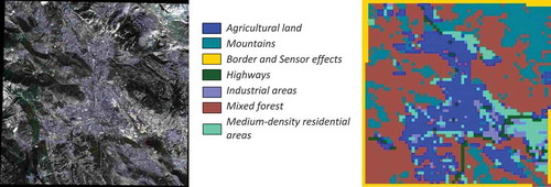
Figure 37. A data set of the French Riviera and its surrounding areas. (From left to right): An RGB quick-look view of a Spot-5 image from April 23rd, 2001, and its classification map. For classification three bands (band 1, 2, and 3) were selected. The sensor parameters are described in Spot sensor parameter description (Spot, 2020)

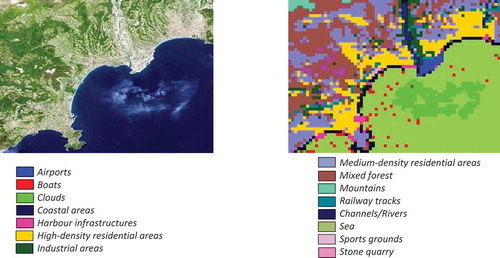
Figure 38. A data set of Venice, Italy and its surrounding areas. (From left to right): An RGB quick-look view of a WorldView-2 image from September 9th, 2012, and its classification map. From the available eight bands of the sensor we used for classification three bands (band 1, 2, and 3). The sensor parameters are described in WorldView sensor parameter description (WorldView, 2020)

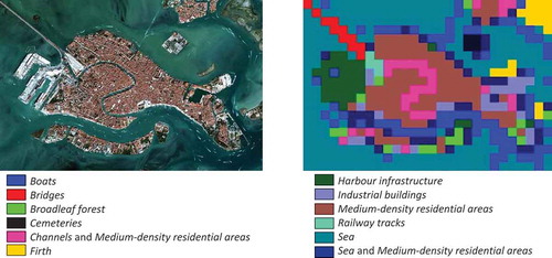
Figure 39. A data set of Calcutta, India (acquired by the Sentinel-3 sensor) and its surrounding areas. (From left to right): An RGB quick-look view of a Sentinel-3 image from January 8th, 2017, and its classification map. From the available 21 bands of the sensor we used for classification eight bands (band 1, 2, 3, 6, 12, 16, 19, and 21). The sensor parameters are described in Sentinel-3 sensor parameter description and data access (Sentinel-3, 2020)

Figure 40. A data set of Amsterdam, the Netherlands and its surrounding areas. (From left to right): A quick-look view of a TerraSAR-X image from May 15th, 2015, and its classification map. The sensor parameters are described in TerraSAR-X sensor parameter description and data access (TerraSAR-X, 2020)

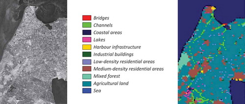
Figure 41. A data set of the Danube Delta, Romania and its surrounding areas. (From left to right): A quick-look view of a COSMO-SkyMed image from September 27th, 2007, and its classification map. The sensor parameters are described in COSMO-SkyMed (COSMO-SkyMed, 2020)

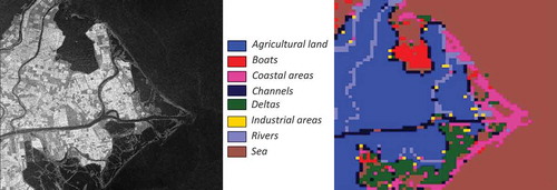
Figure 42. A data set of Vancouver, Canada and its surrounding areas. (From left to right): A quick-look view of a RADARSAT-2 image from April 16th, 2008, and its classification map. The sensor parameters are described in RADARSAT sensor parameter description (RADARSAT, 2020)

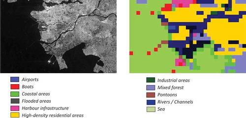
Figure 43. A data set of Berlin, Germany and its surrounding areas. (From left to right): A quick-look view of a Gaofen-3 image from July 27th, 2018, and its classification map. The sensor parameters are described in Gaofen-3 sensor parameter description (Gaofen-3, 2020)

Learning from multi-sensor and multi-temporal data is a way to enrich their content, and to add higher value to the data by appending classification maps, change maps, analytics, etc.

The results of the semantic annotation of the data being used for each use case show how many categories can be extracted from each area depending on the instrument, and also on the geographical and architectural region. During this evaluation, it was also possible to show the influence of the weather on the classifications (in some cases, these data are missing).

In order to fulfil the Big data requirement, Table 4 presents the achievements of the Data Mining module in respect to this requirement, while Table 5 gives for each activity the accomplishment of the Data Mining module.

Table 4. Demonstration of the Big data achievements with the Data Mining module

Big Data	Data Mining achievements
Volume	1 Million square km
Variability	Sentinel-1, Sentinel-2 and 10 other multispectral and SAR EO image types
Velocity	Fast operation (minutes)
Veracity	Training data selected in an active learning loop, very small volume, thus verifiable
Value	Extraction of users/applications adapted to EO image semantics

Table 5. The achievements of the Data Mining module for each activity

CANDELA Activities	Accomplishment by the Data Mining task
Activity 1	Interactive (Active Learning) pattern identification from large geographical scale (about 1 million km2).
Activity 2	Demonstration of the Data Mining on 10 multispectral and SAR images from contributing missions.
Activity 3	Two Data Mining sub-modules have been encapsulated into Dockers and deployed on the CANDELA cloud platform. Users use Jupyter notebooks to launch these processes.
Activity 4	Data Mining archives state-of-the-art (SoA) accuracy, with few training samples (beyond SoA) and very fast (beyond SoA).
Activity 5	Data Mining is processing data, operating with Sentinel-1 and Sentinel-2 products, which was demonstrated in the urban expansion and agriculture use case, forest monitoring use case, and a Big data demonstration.

In summary, our primary conclusions are:

• Our approach is user-friendly (e.g., by rapid active learning).

• Our approach allows multi-target query techniques (metadata, features, semantic labels or combinations thereof).

• We can work with different instrument data (e.g., SAR and multispectral images) and dozens of sensors.

• Features can be optimally extracted with different dedicated state-of-the-art algorithms (e.g., for vegetation, waterbodies, and urban areas).

• Important final products are semantic classification maps, statistical analytics, etc.

• However, our multispectral images are sometimes affected by clouds and often no reliable reference data are available.

As short-term future work, the fusion (Datcu et al., 2019b) of data coming from SAR (e.g., Sentinel-1) and multispectral (e.g., Sentinel-2) data is under validation with the CANDELA platform. The data fusion module is also based on the Data Mining module by adding a component for fusion of radar and multispectral data and features/descriptors with different patch sizes and for fusion of different semantic labels. This will help circumvent Sentinel-2 problems with cloud cover.

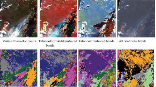
As long-term future work, we plan to combine the two polarizations of the Sentinel-1 instrument and to analyze their influence on the number of additional categories that can be retrieved, and on the quality of these categories. As for Sentinel-2, we will continue to analyze the results already obtained, to see how the influence of different combination of bands that are available for this instrument and whether they can provide a better separation of the different categories (e.g., smoke from clouds), and possibly to increase the number of retrieved categories and their accuracy. As a first example, we show the impact of different band combinations of Sentinel-2 channels. Figure 44 illustrates the band-dependent appearance of Clouds, Smoke, and Fires in the Amazon rainforest (for more details, see also (ESA: Fires ravage the Amazon, 2019)). This study is currently under work and will be published in a future paper.

Figure 44. Visibility of different categories depending on the selection of the Sentinel-2 color bands. (From left to right, top): A quick-look view of visible false-color bands (B4, B3, and B2), false-colour visible/infrared bands (B8, B4, and B3), false-color infrared bands (B12, B11, and B8A), and all bands (B1, B2, B3, B4, B5, B6, B7, B8, B8A, B9, B10, B11, and B12). (From left to right, bottom): An example that shows four combination of bands and the information that can be extracted (Espinoza-Molina, Bahmanyar, Datcu, Díaz-Delgado, & Bustamante, 2017)

Acknowledgments

The work was supported by the European Commission’s H2020 CANDELA project under Grant Agreement No. 776193. We would like to thank our colleagues Wei Yao, Fabien Castel, Jean Francois Rolland, and the other partners from the CANDELA project for their support and advice, and to Gabriel Dax master student in our group from Salzburg University of Applied Sciences, for his first validation tests.

Data availability statement

For the moment, the data from the project are not publicly available. The data that support the findings of this study will be available on request from the authors.

Disclosure statement

No potential conflict of interest was reported by the authors.

Additional information

Notes on contributors

Corneliu Octavian Dumitru

Corneliu Octavian DUMITRU received the B.S. and M.S. degrees in Applied Electronics from the Faculty of Electronics, Telecommunications and Information Technology and the Ph.D. degree in Engineering both from Politehnica University Bucharest, Bucharest, Romania, in 2001, 2002, and 2006, respectively, and the Ph.D. degree in Telecommunications from Pierre and Marie Curie University, Paris, France, in 2010.

From 2005 to 2006, and in 2008, he was a Coordinator for two national grants delivered by the Romanian Ministry of Education and Research.

Since 2010, he has been a Scientist with the Remote Sensing Technology Institute, German Aerospace Center, Oberpfaffenhofen, Germany. At the Politehnica University, he had a teaching activity as a Lecturer, delivering lectures and seminaries and supervising laboratory works in the fields of information and estimation theory, communication theory, and signal processing.

Since 2004, he has been co-supervising internships, master, and Ph.D. theses.

He is currently involved in several projects in the frame of the European Space Agency and European Commission Programmes for information extraction, taxonomies, and data mining and knowledge discovery using remote sensing imagery. His research interests include stochastic process information, model-based sequence recognition and understanding, basics of man–machine communication, information management, and image retrieval in extended databases.

Gottfried Schwarz

Gottfried SCHWARZ received the Graduate degree from the Technical University of Munich, Munich, Germany, in 1976.

For many years, he has been involved in a number of national and international space projects with the German Aerospace Center, Oberpfaffenhofen, Germany; among them were deep-space missions as well as Earth observation missions.

In particular, he has been involved in the design of deep-space instruments from initial engineering studies to detailed design work, modeling of instrument performance, instrument assembly and testing, real-time experiment control, instrument check-out and calibration, data verification and validation, as well as data processing and scientific data analysis. Besides instrument-related aspects, he has also many years of experience in the processing and analysis of various instrument data within ground segments, in particular of optical and SAR remote sensing data, in the interpretation of geophysical data with emphasis on retrieval algorithms with forward modeling, inversion techniques, and data mining.

Special experience in signal processing resulted from engagement in image data compression and feature analysis together with performance analysis of image classification.

Anna Pulak-Siwiec

Anna PULAK-SIWIEC holds a MSc degree in Geodesy and Cartography (specialization: Geoinformatics, Photogrammetry and Remote Sensing) from the AGH University of Science and Technology in Krakow, Poland. Since 2017 she has been working in the Aviation Technologies and Remote Sensing Department of SmallGIS company, where she is engaged in research projects including several ones financed by The National Centre for Research and Development in Poland. Her professional interest focuses on application of remote sensing techniques for needs of agriculture, forest management, and environmental protection.

Bartosz Kulawik

Bartosz KULAWIK is the International Project Coordinator at SmallGIS company. He holds a degree in Geography and Spatial Planning from the Jagiellonian University in Cracow, Poland. Currently, he is conducting his Ph.D. thesis at this same faculty. Since 2010, Mr. Kulawik has been the Market Development Director at SmallGIS, focused mainly on developing remote sensing satellite methods for a variety of Polish and European users. He was a project coordinator for UrbanSAT which was conducted in a previous PECS call. At this time, he was employed at the Polish Space Research Center as a project coordinator. The project was finished with very good success, with its perspective implementation for other beneficiaries in Poland. In 2012, he finished his postgraduate studies in regard to the management of research projects and the commercialization of research results at the Economic University in Cracow.

Mohanad Albughdadi

Mohanad ALBUGHDADI received his B.Sc. in Computer Engineering from IUG in Palestine in 2010. In 2011, he attained his M.Sc. in Electronic Systems Design Engineering from the University of Science in Malaysia. After obtaining the French government scholarship to pursue his doctoral degree, he obtained his Ph.D. in signal, image, acoustics and optimization from ENSEEIHT (the National Polytechnic Institute of Toulouse), and the IRIT laboratory in France in 2016. During his research tenure, he worked as a PostDoc at the IRIT laboratory in the framework of the SparkinData project for developing agricultural applications such as crop classification and anomaly detection using satellite images and machine learning. For the time being, he works at TerraNIS as the Responsible for AI and Digital Transformation unit where he leads the development of machine learning and deep learning applications on various data sources with a focus on satellite images as well as the management of the company’s services on Google Cloud. His research focuses on image and signal processing, data analysis, supervised and unsupervised learning as well as Bayesian inference.

Jose Lorenzo

Jose LORENZO joined in January 2020 the Financial and Incentive Office in Atos Research & Innovation (ARI). Former Head of the Manufacturing, Retail and Environment Market and previously E&U Market Manager also in ARI. He has a Telecommunication Engineer Degree (Master of Science) and specialty of TELEMATICA (Data Transmission) by the Faculty of Technology in the University of Vigo (Spain). He joined the former ATOS, Sema Group sae, in April 2001 as a Consultant. Since then, he has been involved in the technical development, management and coordination of EU funded projects, like ORCHESTRA or DEWS, in the areas of Environmental Risk Management. The latest projects being coordinated by him were EO2HEAVEN (as Research Coordinator), OpenNode or ENVIROFI (phase 1 project of the FI-PPP), and more recently EO4wildlife (http://eo4wildlife.eu) or CANDELA (http://candela-h2020.eu), both funded under the Earth Observation topic of the European Space theme.

Mihai Datcu

Mihai DATCU received the M.S. and Ph.D. degrees in Electronics and Telecommunications from the University Politechnica Bucharest (UPB), Romania, in 1978 and 1986. In 1999 he received the title Habilitation à diriger des recherches in Computer Science from University Louis Pasteur, Strasbourg, France. Currently, he is a Senior Scientist and Image Mining research group leader with the Remote Sensing Technology Institute of the German Aerospace Center (DLR), and Professor with the Department of Applied Electronics and Information Engineering, Faculty of Electronics, Telecommunications and Information Technology, UPB. From 1992 to 2002 he had a longer Invited Professor assignment with the Swiss Federal Institute of Technology, ETH Zurich. From 2005 to 2013 he has been Professor holder of the DLR-CNES Chair at ParisTech, Paris Institute of Technology, Telecom Paris. His interests are in Data Science, Machine Learning and Artificial Intelligence, and Computational Imaging for space applications. He is involved in Big Data from Space European, ESA, NASA and national research programs and projects. He is a member of the ESA Big Data from Space Working Group. In 2006, he received the Best Paper Award of the IEEE Geoscience and Remote Sensing Society. He is the holder of a 2017 Blaise Pascal Chair at CEDRIC, CNAM, France.

References

- Airbus Space and Defense, sample imagery. 2020. Retrieved from https://www.intelligence-airbusds.com/en/8262-sample-imagery
- Aubrun, M., Troya-Galvis, A., Albughdadi, M., Hugues, R., & Spigai, M. (2020). Unsupervised learning of robust representations for change detection on Sentinel-2 earth observation images. The 13th International Symposium on Environmental Software Systems, Wageningen, Netherlands. 1–4.
- Blanchart, P., Ferecatu, F., Cui, S., & Datcu, M. (2014). Pattern retrieval in large image databases using multiscale coarse-to-fine cascaded active learning. IEEE Journal of Selected Topics in Applied Earth Observations and Remote Sensing, 7(4), 1127–1141.
- Candela. (2019). Copernicus access platform intermediate layers small scale demonstrator) project. Retrieved from http://www.candela-h2020.eu/
- Chen, J., Shan, S., He, C., Zhao, G., Pietikäinen, M., Chen, X., & Gao, W. (2010). WLD: A robust local image descriptor. IEEE Transactions on Pattern Analysis and Machine Intelligence, 32(9), 1705–1720.
- CORDIS. (2019). EU research results of the European commission. Retrieved from https://cordis.europa.eu/programme/rcn/701821/en
- COSMO-SkyMed. (2020). Retrieved from https://www.e-geos.it/#/satellite-hub/general/satellite-detail/csk
- CreoDIAS. (2019). Retrieved from https://creodias.eu/
- D. Powers. (2011). Evaluation: From precision, recall and F-measure to ROC, informedness, markedness & correlation. Journal of Machine Learning Technologies, 2(1), 37–63.
- Datcu, M., Dumitru, C. O., & Yao, W. (2019a, October 2). Data mining v2. Candela Deliverable D2. 34. Retrieved from http://www.candela-h2020.eu/content/data-mining-v2
- Datcu, M., Dumitru, C. O., & Yao, W. (2019b, October 8). Data Fusion v2. Candela Deliverable D2. 36. Retrieved from http://www.candela-h2020.eu/content/data-fusion-v2
- Datcu, M., Grivei, A. C., Espinoza-Molina, D., Dumitru, C. O., Reck, C., Manilici, V., & Schwarz, G. 2020. The digital earth observation librarian: A data mining approach for large satellite images archives. Big Earth Data, 1–30. doi:10.1080/20964471.2020.1738196
- Dax, G. (2019, August). Supervised and unsupervised methods in data mining. (Master’s Thesis). Salzburg University of Applied Sciences.
- DIAS platform. 2020. Retrieved from https://www.copernicus.eu/news/upcoming-copernicus-data-and-information-access-services-dias
- Dorne, J., Aussenac-Gilles, N., Comparot, C., Hugues, R., Planes, J.-G., & Trojahn, C. (2020). Une approche sémantique pour représenter l’indice de végétation d’images Sentinel-2 et son evolution. The 13th International Symposium on Environmental Software Systems, Wageningen, Netherlands. 1–4 (in French).
- Dumitru, C. O., Andrei, V., Schwarz, G., & Datcu, M. (2019). Machine learning for sea ice monitoring from satellites, Photogrammetric Image Analysis & Munich Remote Sensing Symposium. Munich, Germany, XLII-2/W16, 83–89. Retrieved from https://www.int-arch-photogramm-remote-sens-spatial-inf-sci.net/XLII-2-W16/83/2019/
- Dumitru, C. O., Cui, S., Schwarz, G., & Datcu, M. (2015). Information content of very-high-resolution SAR images: Semantics, geospatial context, and ontologies. IEEE Journal of Selected Topics in Applied Earth Observations and Remote Sensing, 8(4), 1635–1650.
- Dumitru, C. O., & Datcu, M. (2013). Information content of very high resolution SAR images: Study of feature extraction and imaging parameters. IEEE Transactions on Geoscience and Remote Sensing, 51(8), 4591–4610.
- Dumitru, C. O., Schwarz, G., & Datcu, M. (2016). Land cover semantic annotation derived from high-resolution SAR images. IEEE Journal of Selected Topics in Applied Earth Observations and Remote Sensing, 9(6), 2215–2232.
- Dumitru, C. O., Schwarz, G., & Datcu, M. (2018). SAR image land cover datasets for classification benchmarking of temporal changes. IEEE Journal of Selected Topics in Applied Earth Observations and Remote Sensing, 11(5), 1571–1592.
- Envisat sensor parameter description. (2020). Retrieved from https://earth.esa.int/web/eoportal/satellite-missions/e/envisat
- EOLib project. (2019). Retrieved from http://wiki.services.eoportal.org/tiki-index.php?page=EOLib
- EOWEB GeoPortal TerraSAR-X/TanDEM-X data. (2020). Retrieved from https://eoweb.dlr.de/egp/
- ESA: Fires ravage the Amazon. (2019, August). Retrieved from https://www.esa.int/Applications/Observing_the_Earth/Copernicus/Sentinel-3/Fires_ravage_the_Amazon
- Espinoza-Molina, D., Bahmanyar, R., Datcu, M., Díaz-Delgado, R., & Bustamante, J. (2017). Land-cover evolution class analysis in Image Time Series of Landsat and Sentinel-2 based on Latent Dirichlet Allocation. The 9th International Workshop on the Analysis of Multitemporal Remote Sensing Images (MultiTemp), Brugge, Belgium, 1–4.
- European Commission. (2019). Retrieved from https://ec.europa.eu/info/events/h2020-eo-big-data-hackathon-2019-nov-07_en
- Free satellite data list. 2020. Retrieved from https://gisgeography.com/free-satellite-imagery-data-list/
- Free satellite imagery data sources. (2020). Retrieved from https://eos.com/blog/7-top-free-satellite-imagery-sources-in-2019/
- Gaofen-3 sensor parameter description. (2020). Retrieved from https://directory.eoportal.org/web/eoportal/satellite-missions/g/gaofen-3
- Georgescu, F., Vaduva, C., Raducanu, D., & Datcu, M. (2016). Feature extraction for patch-based classification of multispectral earth observation images. IEEE Geoscience and Remote Sensing Letters, 13(6), 865–869.
- Google Maps. (2019). Retrieved from http://www.google.com/intl/en_ALL/help/terms_maps.html
- H2020 EO Big Data Shift call. (2020). CANDELA related projects: perceptiveSentinel project, OpenEO project, EOpen project, and BETTER project. Retrieved from http://candela-h2020.eu/related_projects
- Joint Hackathon organized by European Commission in Frascati, Italy. (2019, November 7-8). Retrieved from http://candela-h2020.eu/content/joint-hackathon-organized-eo-2-2017-projects
- Landsat sensor parameter description. (2020). Retrieved from https://landsat.gsfc.nasa.gov/
- Manning, C. D., Raghavan, P., & Schütze, H. (2008). Introduction to information retrieval. Cambridge, UK: Cambridge University Press.
- MonetDB. (2019). Retrieved from https://www.monetdb.org/
- MPEG7. (2019). Retrieved from http://mpeg.chiariglione.org/standards/
- Pléiades sensor parameter description. (2020). Retrieved from https://earth.esa.int/web/eoportal/satellite-missions/p/pleiades
- QuickBird sensor parameter description and data access. (2020). Retrieved from https://www.satimagingcorp.com/satellite-sensors/quickbird/
- RADARSAT sensor parameter description. (2020). Retrieved from https://www.asc-csa.gc.ca/eng/satellites/radarsat/technical-features/radarsat-comparison.asp
- REST API. (2019). Retrieved from https://restfulapi.net/
- Sentinel-1. (2019). Retrieved from https://sentinel.esa.int/web/sentinel/missions/sentinel-1
- Sentinel-2. (2019). Retrieved from https://sentinel.esa.int/web/sentinel/missions/sentinel-2
- Sentinel-3 sensor parameter description and data access. (2020). Retrieved from https://sentinel.esa.int/web/sentinel/user-guides/sentinel-3-olci
- Spot sensor parameter description. (2020). Retrieved from https://earth.esa.int/web/eoportal/satellite-missions/s/spot-6-7
- Sumbul, G., Charfuelan, M., Demir, B., & Markl, V. (2019). BigEarthNet: A large-scale benchmark archive for remote sensing image understanding. IEEE International Geoscience and Remote Sensing Symposium, Yokohama, Japan, 5901–5904.
- TanDEM-X sensor parameter description and data access. (2020). Retrieved from https://tandemx-science.dlr.de/cgi-bin/wcm.pl?page=Tdm-Science-Team-Meeting
- TerraSAR-X sensor parameter description and data access. (2020). Retrieved from https://sss.terrasar-x.dlr.de/
- Thematic Exploitation Platforms. (2020). Retrieved from https://eo4society.esa.int/thematic-exploitation-platforms-overview/
- WorldView sensor parameter description. (2020). Retrieved from https://www.satimagingcorp.com/satellite-sensors/worldview-2/