Clustering spatio-temporal bi-partite graphs for finding crowdsourcing communities in IoMT networks

ABSTRACT

The Internet of Moving Things is rapidly becoming a reality where intelligent devices and infrastructures are fostering real-time data sustainability in smart cities and advancing crowdsourced tasks to improve energy consumption, waste management, and traffic operations. These intelligent devices create a complex network scenario in which they often move together or in conjunction with one another to complete crowdsourced tasks. Our research premise is that mobility relationships matter when performing these tasks, and therefore, a graph model based on representing the changes in mobility relationships is needed to help identify the neighbour devices that are moving close to one another in our physical world but also seamlessly connected in their virtual world. We propose a bi-partite community mobility graph model for linking intelligent devices in both virtual and physical worlds, as well as reaching a trade-off between crowdsourced tasks designed with explicit and implicit citizen participation. This paper aims to explore a bi-partite graph as a promising spatio-temporal representation of IoMT networks since changes in mobility relationships over time can indicate volunteer organisation at the device and community levels. The Louvain community detection method is proposed to find communities of intelligent devices to reveal a value conscious participation of citizens. The proposed bi-partite graph model is evaluated using a real-world scenario in transportation, confirming the main role of evolving communities in developing crowdsourcing IoMT networks.

KEYWORDS:

• Bi-partite graph modelling
• Internet of Moving Things
• crowdsourcing

1. Introduction

Crowdsourcing has been a phenomenon characterised by many overlapping idiosyncratic definitions coming from research fields in volunteered geographic information (Elwood, Goodchild, & Sui, 2012; Senaratne, Mobasheri, Ali, Capineri, & Haklay, 2017), crowd wisdom (Davis-Stober, Budescu, Dana, & Broomell, 2014), collective intelligence (Suran, Pattanaik, & Draheim, 2020), mobile crowd sensing (Guo, Yu, Zhou, & Zhang, 2014; Kazemi et al., 2013; Ogie, 2016), and participatory sensing (Burke, Estrin, Hansen, Parker, Ramanathan, Reddy, Srivastava, 2006; Farkas, 2020); and to date, there is still an absence of shared scientific terms and concepts. The applications of crowdsourcing have been numerous and varied, cutting across a wide range of areas for supporting public processes in planning, decision-making and policy formation activities in public health, education, public safety, environmental monitoring, transportation, and disaster management (Feese, Burscher, Jonas, & Tröster, 2014; Hossain & Kauranen, 2015; Klonner, Marx, Usón, Porto de Albuquerque, & Höfle, 2016; Lashkari, Rezazadeh, Farahbakhsh, & Sandrasegaran, 2019; Sui, Elwood, & Goodchild, 2012).

Independently of its definition or the public process at hand, crowdsourcing raises the notion of distributed tasks being carried out by a large number of anonymous citizens. Having crowdsourced data being generated by citizens are a well-established process in crowdsourcing. This process is mainly carried out when the citizens use their smartphones and wearable devices, which usually have some type of embedded sensors, including an accelerometer, GPS, digital compass, environmental sensors, microphone, gyroscope, and camera (Wazny 2017). As previous research has shown, mobile phones have been unique in providing crowdsourced data for accomplishing the localization, labelling and mapping of events, personal and surrounding contexts, social relationships, and human activities (Annis & Nardi, 2019; Boella et al., 2019; Calabrese, Colonna, Lovisolo, Parata, & Ratti, 2011; Kong et al., 2019; Tong et al., 2016).

The emerging Internet of Moving Things (IoMT) as a new technological infrastructure for sensing and communication is an untried crowdsourcing paradigm, which will not only generate a flood of crowdsourced data at extremely high data rates covering extensive geographical areas, but will also create a complex crowdsourcing network of intelligent devices capable of performing crowdsourced tasks which are not only related in harvesting data, but also evaluating current events, making decisions, and acting upon these decisions (Misra & Narendra, 2016; Xu et al., 2018). A key aspect of IoMT is to have intelligent devices that can communicate with one another to achieve a common crowdsourcing task with either the implicit or explicit participation of a citizen.

Our research premise is that geographical proximity matters in performing crowdsourced tasks in IoMT networks, where moving intelligent devices are expected to be collaborating with one another, and therefore, a graph model is needed to help represent the moving devices that are geographically close to one another in our physical world but also connected in their virtual world. We propose a bi-partite community mobility graph model for linking the intelligent devices in both virtual and physical worlds, and reaching a trade-off between crowdsourced tasks designed with explicit citizen participation (e.g. user control) and implicit citizen participation (e.g. system automation). The changes between the mobility relationships over time will influence the common crowdsourced tasks to be achieved by the intelligent devices. How a virtual world of intelligent devices will conform to citizens’ values and cope with the specific challenges such as transparency and privacy will have a strong impact on the participation of citizens in IoMT networks.

To address this challenge, this research proposes the use of bi-partite graphs as a promising spatio-temporal representation of IoMT networks since mobility relationships can reproduce evolving communities showing a volunteer organisation in two ways: (1) as connected moving devices in a virtual world, performing a pre-defined set of individual crowdsourcing tasks (e.g. connected vehicles on a motorway that are collecting traffic and environmental data); and (2) as a community of connected moving devices that are more likely to interact with each other in the real-world for performing a common crowdsourcing task to address a shared problem (e.g. keep moving on a motorway despite the heavy traffic, or avoid bottlenecks by taking the next exit).

Using bi-partite graphs to represent complex networks has been extensively studied in the past (Boccaletti, Latora, Moreno, Chavez, & Hwang, 2006; Easley & Kleinberg, 2010; Zha et al., 2001), but to the best of our knowledge, there has been no previous research work on exploring bi-partite graphs for modelling mobility relationships and finding communities in crowdsourcing IoMT networks.

This paper explores using the landmark time window model for building evolving bi-partite graphs representing changes in mobility relationships over time. By considering the mobility relationships of the IoMT devices as a key factor when building a bi-partite graph for each time window, the Louvain community detection method is proposed to find communities to reveal the possible participation of citizens. We evaluate our proposed model by simulating a network of connected vehicles moving on a highway during a peak hour.

2. Background and related work

Bi-partite graphs are versatile in their ability to model networks. In fact, all complex networks are considered to have an underlying bi-partite structure (Guillaume & Latapy, 2006). Many networks have a natural bi-partite structure that is clearly apparent in two distinct sets of nodes, known as primary set and secondary set, in such a way that links between nodes may occur only if the nodes belong to different sets. However, no previous research work was found on modelling mobility relationships in crowdsourcing IoMT networks using bi-partite graphs. Objects that move on their own accord can provide potentially more accurate crowdsourced data than static ones, and evolving bi-partite graphs are a promising representation to be explored for finding crowdsourcing communities in IoMT networks, and as a result, more complex crowdsourced tasks can be envisaged.

In this section, we describe the previous research work that we consider related to our proposed approach. Therefore, possibly the most well-known research work on using bi-partite graphs to model a network can be found in Eubank et al. (2004), where a bi-partite graph is proposed to model disease outbreaks in an urban social network. A simulation tool called EpiSims is used to combine estimations of population mobility with a model for simulating the progression of a disease within a host and transmission to another host. The bi-partite graph is used to represent a contact network, which consists of two disjoint sets, one representing people and the other representing locations. An edge connects a person and a location only if the person visited that location. Each edge is also associated with a start time and end time, indicating the duration that the person visited that location. From this bi-partite graph, it can be determined which people visited the same area by finding all people nodes that are two edges apart. A minimum time threshold can also be applied to ensure that these people were in that area for at least that amount of time. The purpose behind the model is to contain major disease outbreaks and therefore prevent the necessity of mass vaccinations, and to hopefully isolate small subsets of the population to prevent the disease from spreading beyond locally on the graph.

Another application area in which bi-partite graphs have been proven to be effective is personal recommendation. Zhou, Ren, Medo, and Zhang (2007) investigate the issue of weighting a bi-partite graph in a resource allocation process by developing a weighted adjacency matrix. Consider a bi-partite graph with independent sets X and Y. The resource flows from the X nodes to the Y nodes, then back from the Y nodes to the X nodes, as shown in Figure 1.

Figure 1. Process example of resource allocation for X nodes: (a) the bi-partite graph, (b) the X and Y projections, and (c) the number of common neighbours in Y and X – Source Zhou et al. (2007)

The result is a weighted adjacency matrix for the corresponding X nodes of the network, as shown below.

$\left(\begin{array}{c}x{ }^{\mathrm{\prime }}\\ y{ }^{\mathrm{\prime }}\\ z{ }^{\mathrm{\prime }}\end{array}\right)=\left(\begin{array}{ccc}11/18& 1/6& 5/18\\ 1/9& 5/12& 5/18\\ 5/18& 5/12& 4/9\end{array}\right)\left(\begin{array}{c}x\\ y\\ z\end{array}\right)$

After defining this method for weighting nodes, it was then used on a user object network to perform recommendations. The algorithm presented for this uses the weighting method described above to determine a value for all uncollected objects of a user. The values are then sorted in descending order for recommendation. The equation below defines the algorithm used to find the value for each object. In the equation, ω_jl represents the weight, a_li represents the initial resource of l with i (1 if an edge exists, 0 otherwise), and n is the number of objects in the network. Note that this equation is used for only 1 user, and for all users in a network it would need to be configured individually for each user.

$f{ }^{\mathrm{\prime }}\left(o_j\right)=\sum _{l=1}^n{w}_{jl}f\left(o_l\right)=\sum _{l=1}^n{w}_{jl}{a}_{li}$

The algorithm was tested using a sample dataset from MovieLens, a system where users rate movies. The network had 1682 movies and 943 users. To test the performance of the algorithms, 90% of the data from MovieLens was used as training data and the other 10% was used as probe data. The algorithm presented, dubbed Network-Based Inference (NBI), performed slightly better than the Global Ranking method and the Collaborative Filtering method in recommending movies to the users of MovieLens.

The utilisation of bi-partite graphs to model small sizes of IoT networks has also been presented in Cisco Systems (2009). This research investigated a small network of three theoretical IoT devices within a smart home environment. The room includes typical household infrastructure such as a bed, a window, an air conditioner, two lights, and a stereo. Given this information, there may be a number of possible service components that could be performed within the room, as shown in the right hand side of Figure 2.

Figure 2. Room with IoT infrastructure and possible service components – Source Cisco Systems (2009)

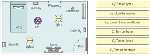
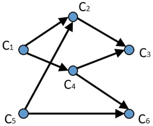
In this specific environment, a number of data flows can be identified and included as part of the environment variables. These flows represent the possible decisions that the IoT network may choose to do given the data they have observed. The data and control flow services for this specific case are shown in Figure 3.

Figure 3. Possible data flows between different service components

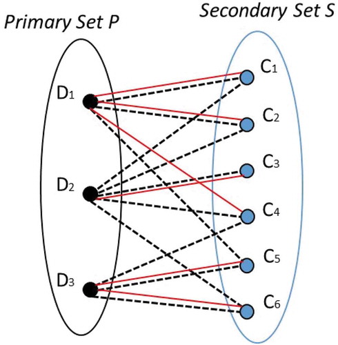
A bi-partite structure is then introduced into the environment, which helps model how each of the devices will help to make service component decisions. The IoT devices D₁, D₂, and D₃ are nodes in the primary set of the bi-partite graph, while the service components C₁, C₂, C₃, C₄, C₅, and C₆ are nodes in the secondary set. Figure 4 shows the structure of this bi-partite graph. The dotted lines represent mappings from service components to IoT devices, and the red lines represent the services for which each device has information. The main contribution of this research, which introduced a new method for sensor selection optimisation, was not ultimately a topic of interest for our research work. However, the conceptualisation presented for modelling IoT devices in a smart home environment as a bi-partite graph was helpful to select the bi-partite modelling approach in our research.

Figure 4. Bi-partite graph representing IoT devices and service components of a smart home environment

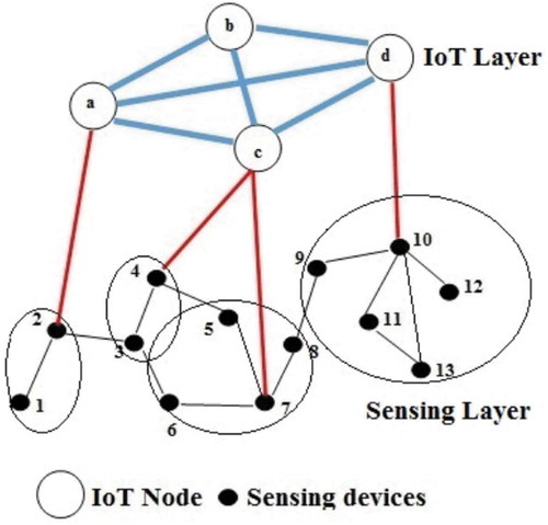
Similarly, there has also been research on using bi-partite graphs to cluster two-tier IoT architectures that contain an IoT layer and a sensing layer (Kumar & Zaveri, 2016). The IoT layer refers to IoT-specific technologies such as edge nodes and fog nodes. These devices are considered to have higher processing, communication, and real-time analysis capabilities. The sensing layer represents devices within the IoT that collect raw data. These devices are IP or ID enabled sensors; they could be general purpose sensing units such as smartphones, video cameras, or accelerometers. The sensing nodes can be grouped using the dominating set, and cluster heads can be chosen, as seen in Figure 5. Cluster heads are tasked with communicating with the IoT layer. This strategy of grouping sensing nodes and designating one node as a cluster head creates a clear bi-partite structure in the network, where the secondary set of nodes is the IoT layer nodes and the other is the primary set. The proposed infrastructure was tested against a very popular clustering algorithm LEACH for flow modelling to achieve fault tolerance with the minimum total energy consumption (Lin, Chelliah, Hsu, & Hou, 2019).

Figure 5. Two-tier infrastructure represented as a bi-partite graph

From a spatial crowdsourcing perspective, Alfarrarjeh, Emrich, and Shahabi (2015) propose a weighted bi-partite graph for matching a set of spatial task nodes with a set of worker nodes using assignment pairs to conform to worker constraints. Some examples of these constraints are the work region where the worker is planning to perform a task, and the maximum number of tasks that a worker is capable of performing. Before building the bi-partite graph, a global geographical area is a-priori selected and partitioned into local areas by using spatial indexing structures such as a Voronoi diagram, a quadtree, or a uniform grid. If a worker region overlaps with a local area, the worker node is replicated in the bi-partite graph. Another important assumption in this approach is that all nodes for all tasks and crowd workers is known before task allocation is performed (i.e. the creation of the links). In the case of the crowdsourcing IoMT networks, the a-priori knowledge of the quantity of intelligent devices is unrealistic.

From a bi-partite clustering perspective, very few community methods have been proposed to take into account the inherent bi-partite complexity of real-world networks. The standard approach is to transform a bi-partite graph into an undirected graph by projecting first the bi-partite structure over one set of nodes, usually using the primary nodes; and then applying standard community detection techniques (Larremore, Clauset, & Jacobs, 2014; Liu & Murata, 2010). However, it has been proven that this approach suffers from limitations due to the loss of information, since it is not possible to determine what is actually preserved when projecting a bi-partite graph. In our proposed bi-partite graph model, the use of projected graphs has been avoided to prevent information loss.

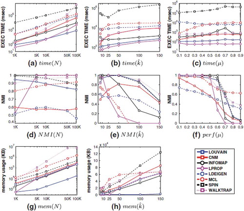
Along with Louvain community clustering algorithm, CNM (Clauset, Newman, & Moore, 2004), Walktrap (Pons & Latapy, 2005), Leading Eigenvector (Newman, 2006), SPIN (Reichardt & Bornholdt, 2006), Label Propagation (Raghavan, Albert, & Kumara, 2007), MCL (van Dongen, 2000), and INFOMAP (Rosvall & Bergstrom, 2008) have been applied in bi-partite graphs. Papadopoulos, Kompatsiaris, Vakali, & Spyridonos (2011) compare those using dataset representative of social media networks. The algorithms are evaluated based on their runtime, normalized mutual information (NMI), and memory consumption. NMI is a metric that provides some feedback as to the quality of the communities produced. The algorithms are also tested based on three important parameters that define the graphs with which they are meant to be used: number of nodes, N, average degree of nodes, $\stackrel{\wedge }{k}$, and mixing parameter, μ. Figure 6 shows how each of the algorithms performed in relation to these parameters. In terms of execution time, Louvain is consistently one of the fastest algorithms along with Label Propagation, regardless of the variation in N, $\stackrel{\wedge }{k}$, or μ. When looking at memory consumption, Figure 6 (g,h), Louvain uses the least amount of memory by a significant margin in both the case of N and $\stackrel{\wedge }{k}$. When looking at the NMI, Louvain attains a high value for the cases of N and $\stackrel{\wedge }{k}$, however there is a significant decline at around 0.7 μ. This is to be expected, as the drop occurs in all of the algorithms. From this, we can see that Louvain is a comparatively fast algorithm that uses little memory and results in good quality community structures.

Figure 6. Comparison of community detection algorithms – Source Papadopoulos et al. (2011)

Studying how communities change over time in a given network has also been a topic of interest to researchers. There are generally two strategies available to study how communities change over time: the first is taking snapshots of the network at different times and comparing them, and the second is to use temporal information directly in the community detection. Aynaud and Guillaume (2010) has explored the Louvain community detection algorithm to solve the problem with computing communities from one timestamp to the next. The results show that the generic Louvain algorithm is very unstable, meaning that the addition and subtraction of nodes into the network drastically changes the resulting communities found. To address this, a stabilized version of the algorithm is proposed in this paper. While the original Louvain algorithm starts with every node in its own community, we have modified the algorithm so that, instead of creating new communities at each timestamp, the communities from time t – 1 would be used as the initial communities for time t. This allows for better tracking of communities and how they change as time progresses.

3. Bi-partite community mobility graph model

The proposed approach is based on making use of bi-partite graph modelling to represent mobility relationships that play an important role in performing crowdsourcing tasks at the community level of an IoMT network. The assumption is that the devices belonging to a community can communicate with one another to achieve a crowdsourcing task during a time interval, having either the implicit or explicit participation of a citizen.

3.1. Defining mobility relationships over time

The movement of an IoMT device is usually recorded as a data point P containing a massive sequence of unbounded tuples t at a rapid rate, which can be formalised as a multidimensional vector where n is the dimensionality of the feature space:

$P=⟨t_1,t_2,\dots ,t_n⟩$

where;

$t_1=\left(id,x_1,y_1,v_1,t{s}_1,\right);$

$t_2=\left(id,x_2,y_2,v_2,t{s}_2,\right);$

$t_n=\left(id,x_n,y_n,v_n,t{s}_n,\right)$

where;

- $id:\mathrm{u}\mathrm{n}\mathrm{i}\mathrm{q}\mathrm{u}\mathrm{e}\mathrm{i}\mathrm{d}\mathrm{e}\mathrm{n}\mathrm{t}\mathrm{i}\mathrm{f}\mathrm{i}\mathrm{e}\mathrm{r}\mathrm{o}\mathrm{f}\mathrm{a}\mathrm{n}\mathrm{I}\mathrm{o}\mathrm{M}\mathrm{T}\mathrm{d}\mathrm{e}\mathrm{v}\mathrm{i}\mathrm{c}\mathrm{e}$;

- $x_n,y_n:\mathrm{g}\mathrm{e}\mathrm{o}\mathrm{g}\mathrm{r}\mathrm{a}\mathrm{p}\mathrm{h}\mathrm{i}\mathrm{c}\mathrm{a}\mathrm{l}\mathrm{c}\mathrm{o}\mathrm{o}\mathrm{r}\mathrm{d}\mathrm{i}\mathrm{n}\mathrm{a}\mathrm{t}\mathrm{e}\mathrm{s}\mathrm{o}\mathrm{f}\mathrm{t}\mathrm{h}\mathrm{e}\mathrm{l}\mathrm{o}\mathrm{c}\mathrm{a}\mathrm{t}\mathrm{i}\mathrm{o}\mathrm{n}\mathrm{o}\mathrm{f}\mathrm{t}\mathrm{h}\mathrm{i}\mathrm{s}\mathrm{d}\mathrm{e}\mathrm{v}\mathrm{i}\mathrm{c}\mathrm{e}$;

- $v_n:\mathrm{v}\mathrm{e}\mathrm{l}\mathrm{o}\mathrm{c}\mathrm{i}\mathrm{t}\mathrm{y}\mathrm{o}\mathrm{f}\mathrm{t}\mathrm{h}\mathrm{e}\mathrm{I}\mathrm{o}\mathrm{M}\mathrm{T}\mathrm{d}\mathrm{e}\mathrm{v}\mathrm{i}\mathrm{c}\mathrm{e}$;

- $t{s}_n:\mathrm{t}\mathrm{i}\mathrm{m}\mathrm{e}\mathrm{s}\mathrm{t}\mathrm{a}\mathrm{m}\mathrm{p}$

From a temporal perspective, the tuples arrive continuously and a time window model is necessary for extracting small and quasi-static subsets of tuples for incrementally codifying a mobility relationship. The main time window models proposed in the literature are damped, sliding, and landmark. The damped model assigns a weight to each arriving tuple from a data stream, while over time the weights of older tuples decay by an exponential fading factor, which gives a higher importance to recent tuples. However, this time window model does not discard any tuple, making its use challenging for creating mobility relationships over time, since all data points will be always active.

In the sliding time window model, a fixed time interval is used, and as time goes by, the window slides by considering the most recent tuples where the older tuples are removed once new tuples are available. The time interval can be defined in terms of the last arrived tuples (e.g. the last 100,000 recorded tuples) or a fixed time duration (e.g. the last 5 minutes). Therefore, old and new tuples will coexist within an active window, hampering its use for representing current mobility relationships.

The landmark time window model separates the tuples based on a landmark time interval (e.g. every minute) or by a landmark event (e.g. no vehicles on a highway), when after a landmark is reached, new tuples start to be captured in a separate window. This strategy is particular advantageous for defining mobility relationships among new data points since it creates a sequence of time orderly snapshots. Once a set of new tuples has been gathered for an active window, the mobility relationships among IoMT devices can be determined by the k closest neighbours to a parent device, generating an evolution of mobility relationships over time.

It is important to point out that a mobility relationship is a specific type of spatial relationship, since most of the spatial relationships are usually multidirectional in nature and points are located independently from each other, representing a dispersed and random point distribution. The mobility of IoMT devices is itself limited to a unidirectional spatial relationship, emphasizing the role of many interactions due to contiguity and distance characteristics that play a role in generating a mobility relationship, which is actually imposed between moving neighbours.

3.2. Computing mobility neighbourhoods

We propose the creation of a buffer zone around each IoMT device for ensuring all devices have a neighbour in the virtual-world. This is achieved by formulating a constant contiguity radius r for any data point within a time window. The selected value for a radius r should never be larger than the transmission range of an IoMT device; otherwise, the other devices will not be able to communicate with this device and share crowdsourcing tasks in the virtual world. Another important factor when setting up the radius is that it will also need to be adjusted to the power level of the battery of the device. Large radii will usually consume more power from the device, leading to a trade-off between transmission range and battery consumption.

The next step is to find mobility relationships consistently with the interactions that are expected to take place among IoMT devices in the real-world. For each buffer zone of a point P belonging to a time window TW_i, a minimum distance d_min between a parent point P and any other point P_i located within its buffer zone is calculated in such a way that all points inside this buffer zone becomes a neighbour of the parent point P. The Euclidean distance is proposed for computing the distances d_min. The main assumption is that the d_min between a parent point and its neighbours within every time window should be d_min ≤ r as follows:

$T{W}_i=⟨P_1,P_2,P_3,\dots P_n⟩$

where;

- $P_1\mathrm{i}\mathrm{s}\mathrm{a}\mathrm{p}\mathrm{a}\mathrm{r}\mathrm{e}\mathrm{n}\mathrm{t}\mathrm{p}\mathrm{o}\mathrm{i}\mathrm{n}\mathrm{t},\mathrm{t}\mathrm{h}\mathrm{e}\mathrm{n}{d}_{min}\left(P_1,P_2\right),d_{min}\left(P_1,P_3\right),\dots ,d_{min}\left(P_1,P_n\right),\mathrm{s}\mathrm{h}\mathrm{o}\mathrm{u}\mathrm{l}\mathrm{d}\mathrm{b}\mathrm{e}$

$smallerthanr;$

- $P_2\mathrm{i}\mathrm{s}\mathrm{a}\mathrm{p}\mathrm{a}\mathrm{r}\mathrm{e}\mathrm{n}\mathrm{t}\mathrm{p}\mathrm{o}\mathrm{i}\mathrm{n}\mathrm{t},\mathrm{t}\mathrm{h}\mathrm{e}\mathrm{n}{d}_{min}\left(P_2,P_3\right),d_{min}\left(P_2,P_3\right),\dots ,d_{min}\left(P_2,P_n\right),\mathrm{s}\mathrm{h}\mathrm{o}\mathrm{u}\mathrm{l}\mathrm{d}\mathrm{b}\mathrm{e}$

$smallerthanr;$

- $P_n\mathrm{i}\mathrm{s}\mathrm{a}\mathrm{p}\mathrm{a}\mathrm{r}\mathrm{e}\mathrm{n}\mathrm{t}\mathrm{p}\mathrm{o}\mathrm{i}\mathrm{n}\mathrm{t},\mathrm{t}\mathrm{h}\mathrm{e}\mathrm{n}{d}_{min}\left(P_n,P_1\right),d_{min}\left(P_n,P_2\right),\dots ,d_{min}\left(P_n,P_n\right),\mathrm{s}\mathrm{h}\mathrm{o}\mathrm{u}\mathrm{l}\mathrm{d}\mathrm{b}\mathrm{e}$

$smallerthanr;$

$\mathrm{w}\mathrm{i}\mathrm{t}\mathrm{h}{d}_{min}\left(P_i,P_n\right)\mathrm{t}\mathrm{h}\mathrm{e}\mathrm{m}\mathrm{i}\mathrm{n}\mathrm{i}\mathrm{m}\mathrm{u}\mathrm{m}\mathrm{E}\mathrm{u}\mathrm{c}\mathrm{l}\mathrm{i}\mathrm{d}\mathrm{e}\mathrm{a}\mathrm{n}\mathrm{d}\mathrm{i}\mathrm{s}\mathrm{t}\mathrm{a}\mathrm{n}\mathrm{c}\mathrm{e}\mathrm{b}\mathrm{e}\mathrm{t}\mathrm{w}\mathrm{e}\mathrm{e}\mathrm{n}{P}_i\mathrm{a}\mathrm{n}\mathrm{d}{P}_n.$

Finally, assigning the neighbours to a parent data point can also depend on the current velocity of the moving IoMT devices. Therefore, the devices that are moving slowly will have smaller d_min, while faster moving devices will have larger d_min. The main assumption that the d_min between a parent point and its neighbours continues to be that d_min ≤ r within every time window. In this case, the rules in Table 1 are applied to determine d_min according to the velocity of the IoMT device at a time instance.

Table 1. Steps to allocate d_min according to the current velocities of IoMT devices

GIVEN the location of all the IoMT devices and their respective velocities in TWi

FOR each parent data point Pi and another data point Pj

IF velocity of Pi and Pj is less than vi

FIND the neighbours with dmin ≤ di

The number of mobility neighbourhoods will vary according to the number of IoMT devices for each time interval. In this case, the crowdsourced tasks will be controlled by the devices, and they will be triggered depending on which mobility neighbourhood they are members of. These crowdsourced tasks are expected to have the explicit participation of citizens.

3.3. Building a bi-partite graph based on changes of mobility relationships

We define a bi-partite graph by an ordered triple < P(G), E(G), S(G) > for each time window TW_i, where P(G) is the non-empty set of vertices representing the parent data points; S(G) is the set of vertices representing the k closest neighbours to a parent data point within a buffer zone r; and E(G) is the edge set of the bi-partite graph representing the mobility relationships (d_min). Figure 7 illustrates a bi-partite graph G = (P, S, E) and its bi-adjacency matrix B where B_ij = 1 provided there is an edge between i and j, or otherwise B_ij = 0.

Figure 7. An example of a bi-partite graph based on mobility relationships between neighbours

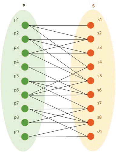
In our bi-partite graph, the number of nodes in P(G) is equal to the number of nodes in S(G), and the two sets P(G) and S(G) have the following properties:

- $\mathrm{I}\mathrm{f}p\in P\left(G\right)\mathrm{t}\mathrm{h}\mathrm{e}\mathrm{n}\mathrm{i}\mathrm{t}\mathrm{c}\mathrm{a}\mathrm{n}\mathrm{o}\mathrm{n}\mathrm{l}\mathrm{y}\mathrm{b}\mathrm{e}\mathrm{a}\mathrm{d}\mathrm{j}\mathrm{a}\mathrm{c}\mathrm{e}\mathrm{n}\mathrm{t}\mathrm{t}\mathrm{o}\mathrm{v}\mathrm{e}\mathrm{r}\mathrm{t}\mathrm{i}\mathrm{c}\mathrm{e}\mathrm{s}\mathrm{i}\mathrm{n}S\left(G\right),$

- $\mathrm{I}\mathrm{f}s\in S\left(G\right)\mathrm{t}\mathrm{h}\mathrm{e}\mathrm{n}\mathrm{i}\mathrm{t}\mathrm{c}\mathrm{a}\mathrm{n}\mathrm{o}\mathrm{n}\mathrm{l}\mathrm{y}\mathrm{b}\mathrm{e}\mathrm{a}\mathrm{d}\mathrm{j}\mathrm{a}\mathrm{c}\mathrm{e}\mathrm{n}\mathrm{t}\mathrm{t}\mathrm{o}\mathrm{v}\mathrm{e}\mathrm{r}\mathrm{t}\mathrm{i}\mathrm{c}\mathrm{e}\mathrm{s}\mathrm{i}\mathrm{n}P\left(G\right),$

- $P\left(G\right)\cap S\left(G\right)=0$

The algorithm for creating a bi-partite graph can be described by the steps in Table 2.

Table 2. Steps to create a bi-partite graph

GIVEN all the data points at a given time window

FOR each parent data point

COMPUTE dmin between the parent data point and other data points

IF dmin < specified user threshold

CREATE edge between parent data point and the other data point

3.4. Finding a mobility community for executing a crowdsourcing task

The Louvain community detection approach is proposed in this research work for finding communities of intelligent devices within a given IoMT network. This approach was chosen because it is a well-established and efficient algorithm to perform clustering (Blondel, Guillaume, Lambiotte, & Lefebvre, 2008). In our bi-partite graph model, the objective is to apply the Louvain algorithm for finding clusters of intelligent devices in an IoMT network that are moving together during a time interval to achieve a common crowdsourcing task. The metric behind measuring how successful the algorithm is at discovering communities is the computing Louvain modularity based on Newman (2006). This modularity measures a ratio of how many edges exist within the community and how many edges exist from the community to other communities in the network, which is defined as follows:

$Q=\frac{1}{2m}\sum _{ij}^0\left[A_{ij}-\frac{k_i{k}_j}{2m}\right]\delta \left(c_i{c}_j\right)$

where

- $2m\mathrm{i}\mathrm{s}\mathrm{t}\mathrm{h}\mathrm{e}\mathrm{s}\mathrm{u}\mathrm{m}\mathrm{o}\mathrm{f}\mathrm{e}\mathrm{d}\mathrm{g}\mathrm{e}\mathrm{w}\mathrm{e}\mathrm{i}\mathrm{g}\mathrm{h}\mathrm{t}\mathrm{s}\mathrm{i}\mathrm{n}\mathrm{t}\mathrm{h}\mathrm{e}\mathrm{g}\mathrm{r}\mathrm{a}\mathrm{p}\mathrm{h};$

- $A_{ij}\mathrm{i}\mathrm{s}\mathrm{t}\mathrm{h}\mathrm{e}\mathrm{e}\mathrm{d}\mathrm{g}\mathrm{e}\mathrm{w}\mathrm{e}\mathrm{i}\mathrm{g}\mathrm{h}\mathrm{t}\mathrm{b}\mathrm{e}\mathrm{t}\mathrm{w}\mathrm{e}\mathrm{e}\mathrm{n}\mathrm{n}\mathrm{o}\mathrm{d}\mathrm{e}\mathrm{s}i\mathrm{a}\mathrm{n}\mathrm{d}j;$

- $k_i\mathrm{a}\mathrm{n}\mathrm{d}{k}_j\mathrm{a}\mathrm{r}\mathrm{e}\mathrm{t}\mathrm{h}\mathrm{e}\mathrm{s}\mathrm{u}\mathrm{m}\mathrm{o}\mathrm{f}\mathrm{w}\mathrm{e}\mathrm{i}\mathrm{g}\mathrm{h}\mathrm{t}\mathrm{s}\mathrm{o}\mathrm{f}\mathrm{t}\mathrm{h}\mathrm{e}\mathrm{e}\mathrm{d}\mathrm{g}\mathrm{e}\mathrm{s}\mathrm{a}\mathrm{t}\mathrm{t}\mathrm{a}\mathrm{c}\mathrm{h}\mathrm{e}\mathrm{d}\mathrm{t}\mathrm{o}\mathrm{n}\mathrm{o}\mathrm{d}\mathrm{e}\mathrm{s}i\mathrm{a}\mathrm{n}\mathrm{d}j;$

- $c_i\mathrm{a}\mathrm{n}\mathrm{d}{c}_j\mathrm{a}\mathrm{r}\mathrm{e}\mathrm{t}\mathrm{h}\mathrm{e}\mathrm{c}\mathrm{o}\mathrm{m}\mathrm{m}\mathrm{u}\mathrm{n}\mathrm{i}\mathrm{t}\mathrm{i}\mathrm{e}\mathrm{s}\mathrm{o}\mathrm{f}\mathrm{n}\mathrm{o}\mathrm{d}\mathrm{e}\mathrm{s}i\mathrm{a}\mathrm{n}\mathrm{d}j;$

- $\delta \mathrm{i}\mathrm{s}\mathrm{a}\mathrm{d}\mathrm{e}\mathrm{l}\mathrm{t}\mathrm{a}\mathrm{f}\mathrm{u}\mathrm{n}\mathrm{c}\mathrm{t}\mathrm{i}\mathrm{o}\mathrm{n}.$

Being an optimisation algorithm, it works to optimise the modularity in a network by first placing all nodes in their own community. For each node, i, the change in modularity is computed for removing i from its own community and into the community of each neighbour, j, of i. Once all nodes have been passed through once, the community of nodes that have been found are then represented as a new single node that turns any links within the cluster into a self-weight, and converts links from cluster to cluster into a weighted edge. The process is reiterated until the modularity is optimized.

The algorithm for creating communities in a given IoMT network starts by placing each node (i.e. IoMT device) in its own community. The change in modularity is tested for transferring a node to another community. If the modularity does not increase, it is not transferred. If the modularity is increased, it is transferred. After every node is tested, the communities are reformed into a new node, which contains a self-weight and a weighted edge to other communities. The initial loop is repeated, and the process continues until there is no increase in the modularity. An overview of the steps is given in Table 3.

Table 3. Steps to find communities in IoMT networks

GIVEN a bi-partite graph network

INITIATE by placing every node into its own community

FOR each node

replace node to neighbouring community

recalculate modularity

IF modularity increases

replace device into a new community

ELSE

Keep node in current community

COMBINE communities into new nodes, using self-weights and weighted edges

REPEAT loop above until modularity is optimized

The number of communities will vary over time, and the crowdsourced tasks will be performed by the IoMT devices, and they will be triggered depending on which community they are members of. These crowdsourced tasks are expected to have the implicit participation of citizens.

3.5. Intrinsic clustering validation

The Silhouette (S) coefficient are proposed to assess the quality of the clustering results since there are no ground true label of data (Arbelaitz et al., 2013). The focus is to determine between-cluster dispersion and inter-cluster dispersion for all clusters. The silhouette width of a data point measures how similar the data point is to its own cluster compared to other clusters. For clusters X_j = (j = 1, … ., c), the silhouette width of the i^th data point in cluster X_j is defined as follows (Rendón, Abundez, Arizmendi, & Quiroz, 2011):

$S\left(i\right)=\frac{\left(b\left(i\right)-a\left(i\right)\right)}{max\left\{a\left(i\right),b\left(i\right)\right\}}$

where a(i) is the average distance between the i^th data point and all data points included in X_j; b(i) is the minimum average distance between the i^th data point and all of the data points clustered in X_k = (k = 1; … c, k ≠ j).

From individual silhouette width calculations, an aggregated global silhouette index is obtained (Petrovic, 2006). The silhouette index values range from −1 to 1 where a value closer to 1 indicates clusters are well separated and clearly distinguished, which relates to a standard concept of a cluster. A value closer to −1 indicates data points are not properly clustered. However, it has a high computational complexity of O(n2).

4. Real-world scenario

We propose a real-world scenario for illustrating a network of smart cars, which are heavily congested on a highway, and are able to communicate using a short range communication network of r = 50 m. In this scenario, each smart car is performing an individual crowdsourced task that consists of harvesting environmental data generated from sensors such as temperature, humidity, and CO₂ sensors located in a smart car. At any time when the smart cars are moving close to each other (d_min ≤ d_i), they are expected to communicate with each other and perform common crowdsourced tasks with the explicit or implicit participation of the drivers and according to the mobility neighbourhood and the communities they belong to. At the mobility neighbourhood level, the crowdsourcing can be aimed at implicitly sharing velocity data among neighbours for addressing a shared problem such as avoiding bottlenecks when taking the next exit. At the community level, the crowdsourced tasks are needed to harvest and share velocity data at the highway network level for addressing a complex issue such as maintaining the velocity on the highway during heavy traffic.

The dataset used to simulate the displacement of this network of smart cars over time was originally collected for the Next Generation Simulation program (NGSIM) in the year 2005 using eight synchronised cameras overlooking a total of 640 metres of Highway 101 in the United States, as shown in Figure 8.

Figure 8. US highway 101 segment used for our real-world scenario

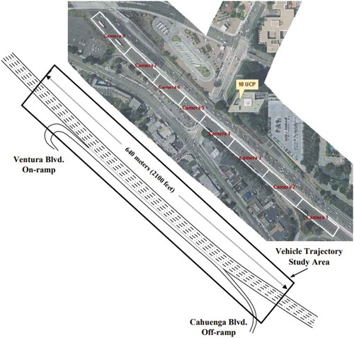
Detailed information about every vehicle on the highway was collected every millisecond second. High-resolution mobility data such as this is similar to what we expect to encounter in the near future in an IoMT network of smart cars. The aerial photograph above shows the extent of the highway segment in relation to the building from which the digital video cameras were mounted and the coverage area for each of the eight cameras. The schematic drawing on the bottom shows the five lanes and the location of the on-ramp and off-ramp.

The data being generated from a smart car are a time series containing information about the smart car identifier, the epoch time elapsed time since Jan 1, 1970, the Global X coordinate of the front centre of the vehicle based on CA State Plane III in NAD83, the Global Y coordinate of the front centre of the vehicle based on CA State Plane III in NAD83, and the instantaneous velocity of the vehicle, as illustrated in Table 4.

Table 4. Example of IoMT data collected by a smart car

Smart Car ID	Epoch Time (milliseconds)	Global X (meters)	Global Y (meters)	Velocity (meter/second)
2	1,118,846,980,300.00	6,451,140.33	1,873,342.00	40.00
2	1,118,846,980,400.00	6,451,143.02	1,873,339.04	40.00
2	1,118,846,980,500.00	6,451,145.71	1,873,336.08	40.00
2	1,118,846,980,600.00	6,451,148.40	1,873,333.12	40.00
2	1,118,846,980,700.00	6,451,151.08	1,873,330.15	40.00
2	1,118,846,980,800.00	6,451,153.77	1,873,327.19	40.00
2	1,118,846,980,900.00	6,451,156.46	1,873,324.23	40.02
2	1,118,846,981,000.00	6,451,159.15	1,873,321.27	40.03
2	1,118,846,981,100.00	6,451,161.84	1,873,318.31	39.93
2	1,118,846,981,200.00	6,451,164.55	1,873,315.32	39.61
2	1,118,846,981,300.00	6,451,167.20	1,873,312.38	39.14
2	1,118,846,981,400.00	6,451,169.80	1,873,309.53	38.61
2	1,118,846,981,500.00	6,451,172.36	1,873,306.72	38.28
2	1,118,846,981,600.00	6,451,174.96	1,873,303.87	38.42
2	1,118,846,981,700.00	6,451,177.61	1,873,300.93	38.78
2	1,118,846,981,800.00	6,451,180.34	1,873,297.92	38.92
2	1,118,846,981,900.00	6,451,182.98	1,873,294.96	38.54
2	1,118,846,982,000.00	6,451,185.54	1,873,292.12	37.51
2	1,118,846,982,100.00	6,451,188.02	1,873,289.41	36.34
2	1,118,846,982,200.00	6,451,190.42	1,873,286.82	35.50
2	1,118,846,982,300.00	6,451,192.76	1,873,284.25	35.08
2	1,118,846,982,400.00	6,451,195.11	1,873,281.66	34.96
2	1,118,846,982,500.00	6,451,197.46	1,873,279.07	34.98
2	1,118,846,982,600.00	6,451,199.81	1,873,276.47	35.00
2	1,118,846,982,700.00	6,451,202.17	1,873,273.88	34.99

The data were aggregated to one second time resolution due to computational power constraints. Afterwards, the aggregated data were broken into eight landmark time windows up to the fifteen minute time period, having approximately 338 seconds each. Three fifteen-minute periods were selected for implementing our real-world scenario. They were as follows: 7:50:00 h to 8:05:00 h; 8:05:01 h to 8:20:00 h; and 8:20:01 h to 8:35 h.

The next steps consisted the computation of the d_min for each time window, and subsequently, the identification of all the neighbours for each smart car in order to build the bi-partite graph. It was determined that the thresholds for d_min would be equal to 5, 10, 15, 20, 25, and 50 m in order to build different bi-partite graphs, and examine the impact these changes have on defining and performing crowdsourcing tasks.

Once the mobility neighbourhoods were created at each instance in time and the neighbours of each smart car were found, the algorithm creates a bi-partite graph at each instance in time. The two set of disjoint nodes are the smart vehicles on the highway and their neighbours. See Table 1 for the sequence of steps for creating a bi-partite graph. The first step was to load the csv file from the previous step. All of the columns are appended to new lists. All of the lists, except the neighbours list, are then aggregated together in a Pandas data frame. All of the unique vehicle ID’s for this time window are then found and converted to strings so they can be compared to the other strings within the neighbour’s lists.

Finally, a nested loop is created to iterate through all of the vehicle ID’s and all of the neighbour lists to verify if the vehicles are within each mobility neighbourhood. If they are, a new row is appended to several lists which indicates the vehicle id, neighbourhood id, x position, y position, velocity, and time. After checking every vehicle against every mobility neighbourhood, all the lists are aggregated and saved into a text file. This text file contains every node pair (vehicle and its neighbour) that make up all of the edges for the bi-partite graphs from the start time to the end time at one second intervals. From this text file we can specify all of the nodes and edges at each instance in time to create a bi-partite graph every one second.

The final step of the algorithm is to compute the communities of smart cars on the highway using the Louvain community detection algorithm. In this case, the algorithm starts by importing the data, which is a text file containing all of the nodes (i.e. vehicles and its neighbours) and their corresponding edges. A new column is created, called edges, which contains these nodes. Empty dictionaries and lists for storing values are created and then a loop begins which iterates from the start time to the end time at one second intervals. The bi-partite graph with two sets of disjoint nodes (one being the vehicle ID’s and one being its neighbour’s ID) is created using the networkx package. To complete the graph, the algorithm inserts the edge connections using the edges column, which contains the tuples of edges.

We have also used an implementation of Louvain clustering known as community best partition, which is provided within the networkx library. The algorithm implements Louvain using the same steps that are described in Section 3.3. Additional steps in the loop calculate some descriptive statistics about the created clusters, such as how many clusters are on the highway, the average number of vehicles per cluster, and the variance in the number of vehicles per cluster.

5. Discussion of the results

The bi-partite graphs were generated every second, and the image in Figure 9 is an example of a how dense a bi-partite graph created at one instance in time can be. If we look more closely at the graph, we can see that a sample of a set of nodes that represents the smart car ID’s (i.e. parent data points) and the right set of nodes represents their neighbours. Edges exist between smart cars and their neighbours when they are moving within the bounds of their mobility relationships. Bi-partite graphs like this one were created successfully for every one second.

Figure 9. Example of a bi-partite graph of smart vehicles and their neighbours moving on highway

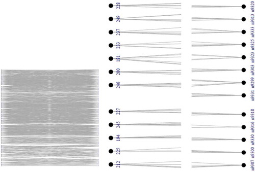
This large-scale bi-partite structure certainly provides a unique spatio-temporal representation based on generating a sequence of connected nodes and edges that indicate the frequency of their mobility relationships. Finding the underlying bi-partite structure over time has many uses in crowdsourcing IoMT networks, including partitioning a whole IoMT network into mobility neighbourhoods for performing common crowdsourcing tasks that depends on smart cars moving close to one another. We anticipate that explicit participation of citizens (in our scenario, the drivers), will be paramount for developing meaningful crowdsourcing tasks. For example, the smart cars approaching the off-ramp would belong to the same mobility neighbourhood, and a common crowdsourcing task consisting of sharing data among them would be needed for optimising their velocities and avoiding an exit bottleneck.

Moreover, different communities have emerged over space and time, and finding the underlying community clusters is expected to have many uses in performing crowdsourced tasks by smart cars on a highway, including avoiding traffic jams. The overview of the statistics related to the community detection results is shown in Table 5. We can see that the total number of communities, mean number of communities, and the standard deviation of the number of communities all decrease as the distance (d_min) of the mobility relationships increases. Conversely, the mean number of smart cars per community and standard deviation of smart cars per community increase as we increase the distance (d_min) of the mobility relationships. Looking at the modularity, we see that it is high for d_min ≤ 5 m and then begins to drop as we increase the d_min. This makes sense, since we would have more neighbours as d_min gets larger, and the communities would be less independent. We have also examined other aspects of the communities, such as the total number of communities on the highway, the number of smart cars in the communities, the velocity of the vehicles in the communities, and of course the modularity of the network.

Table 5. Overview of the community detection results

	5 m	10 m	15 m	20 m	25 m	50 m	Modifiable
Community level
Total number of communities	2943	25650	9842	6312	5099	3421	9450
Maximum number of communities	68	52	22	13	10	6	28
Mean number of communities every second	40	35	13	9	7	5	13
Standard Deviation	9.51	6.62	2.69	1.54	1.18	0.75	3.40
Mean Modularity	0.97	0.92	0.84	0.77	0.72	0.60	0.82
Community composition for every second
Minimum number of smart cars per community	1	1	1	1	1	1	1
Maximum number of smart cars per community	10	51	69	84	102	128	74
Mean number of smart cars per community	2	6	19	29	36	57	19
Mean velocity of smart cars (m/s)	12	13	13	13	13	13	12
Mean variance of velocity of smart cars	0.91	3.49	5.55	5.86	6.12	6.85	4.91

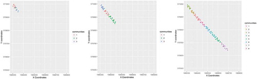
The results on communities in the bi-partite graphs can be seen in Figure 10 where three temporal instances are used to illustrate the evolving communities using d_min = 25 m. As the time passes by, more communities are found containing a larger number of smart cars.

Figure 10. Sequential snapshots of the evolving communities with d_min = 25 m

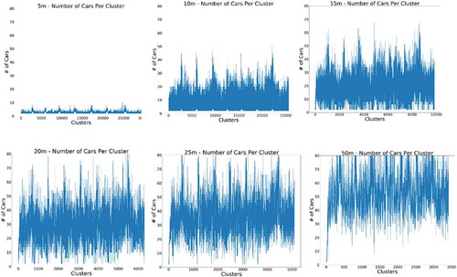
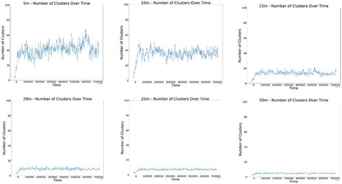
We have also compared the number of communities on the highway over time, and the number of smart cars per each community. Figure 11 shows the number of vehicles in every community for each of the different mobility relationships (d_min). It is clear to see that, as we increase the size of the mobility neighbourhood, not only does the average number of vehicles per community increase, but the noise level within community also increases. Different noise levels occur due to random errors introduced by batch processes when the data are gathered.

Figure 11. Number of connected vehicles discovered in each community (i.e. cluster)

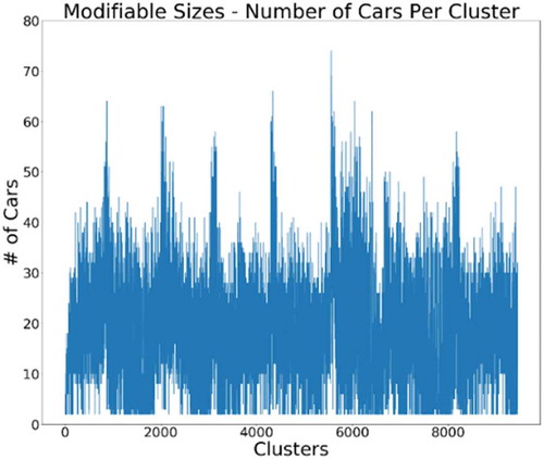
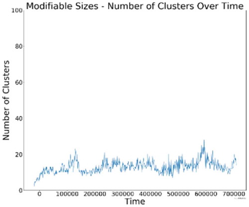
On the other hand, when using the modifiable mobility neighbourhoods, the results closely resemble the patterns shown in the d_min ≤ 15 m, as shown in Figure 12. We would expect the modifiable neighbourhoods to be more similar to the 15 m and 20 m because they are the most common. We can see that the standard deviation in the number of communities is higher for the modifiable neighbourhoods though, indicating that the constant change in d_min makes the number of communities on the highway fluctuate more.

Figure 12. Number of smart cars discovered in each community for modifiable d_min.

We have also examined the number of communities on the highway over time, and the results are shown in Figure 13. Here we see a pattern opposite to that shown in Figure 12 in such a way that the smaller mobility neighbourhoods can cause more of a fluctuation in the number of communities on the highway, while the larger mobility neighbourhoods have a more stable number of communities on the highway.

Figure 13. Number of communities on the highway over time

Interestingly, the modifiable mobility neighbourhoods once again resemble the 15 m pattern, although this time it is clear that there are more fluctuations in the modifiable neighbourhoods (Figure 14).

Figure 14. Number of communities on the highway for modifiable mobility neighbourhoods

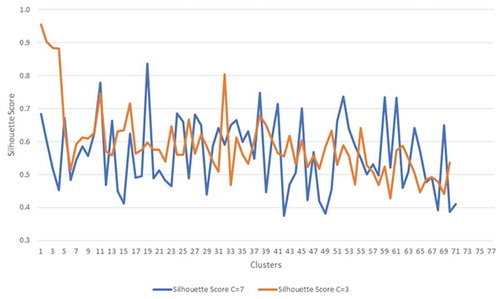
Finally, the silhouette index found in the clustering results have shown that no clusters have been found close to −1. Figure 15 shows the range from 0.38 to 0.98 found in the communities when the total number of clusters were equal 7 (blue line) and 3 (orange line), indicating that the clusters were well separated and clearly distinguished. Similar patterns have also been found for other sizes of communities, providing preliminary empirical results showing that the Louvain community detection algorithm was stable in finding robust clusters throughout the different time windows.

Figure 15. Sample of the generated silhouette index values

6. Conclusions

In this research, the concept of a mobility neighbourhood has been introduced into an IoMT network by creating a bi-partite structure based on changes of mobility relationships over time. We have shown that these bi-partite graphs can then be clustered using the Louvain community detection approach to reveal communities of high modularity. We also experimented with the size of the mobility neighbourhoods to show how this affects the resulting communities, and we show that mobility neighbourhoods can even be built around an existing characteristic of the smart cars, such as velocity.

The real-world scenario was designed to be built upon and there are many ways in which this can be done. For example, when creating edges in our bi-partite graph, we used binary inputs 0 or 1. Future research could involve using weighted edges that are based on proximity and then this method could be compared to our method. Since the mobility relationships are key for discovering communities, more research work will focus on determining the optimised d_min for parameter settings.

Collaboration amongst different fields of academia would also be key in expanding on this proposed approach. In our example of smart cars on a highway, insights from a traffic engineer could help make better decisions regarding the size of mobility neighbourhoods to use, what time intervals to look at, and how to better understand some of the traffic patterns we see happening on the highway. Similarly, another direction in which this work could be expanded is in the realm of physics, namely synchronisation. The level of synchronisation within the Louvain communities could be tested to see if vehicles within communities are in synchronised states. Finally, we will be focusing on incorporating crowdsourced tasks into our model.

Acknowledgments

We thank the anonymous reviewers for their careful reading of our manuscript and their insightful comments and suggestions. We would also like to thank the team of the People in Motion Lab for the fruitful discussions on this research domain.

Data availability statement

The data that support the findings of this study are openly available in Next Generation Simulation (NGSIM) Vehicle Trajectories and Supporting Data (opendatanetwork.com) at https://www.opendatanetwork.com/dataset/data.transportation.gov/.

Disclosure statement

No potential conflict of interest was reported by the author(s).

Additional information

Funding

This research work was supported by the NSERC/Cisco Industrial Research Chair, Grant IRCPJ 488403-1.

Notes on contributors

Kaine Black

Dr. Wachowicz is a world-renowned expert in Geospatial Data Science, with a unique multidisciplinary background in Geography, Geomatics Engineering and Computer Science. She specialises in machine learning for analysing data streams from the Internet of Things, with the purpose of identifying opportunities and challenges in sustainable smart cities. She has collaborated in research projects with many high technology companies, such as IBM, Cisco, Orange Communications, ESRI and Siemens, as well as academics from the USA, Canada, Australia and Europe. Her research has received international recognition through best paper awards from conferences such as ARQUEOLOGICA 2.0, CODS, and AAG; as well as first prize awards in competitions such as Fredericton E-hack Smart City Hackathon and Data Visualization Competition at IBEC. Founding member of the Technical Committee on Big Data of the IEEE Communications Society, and the International Journal of Big Data Intelligence, she has over 250 publications. Her pioneering work in multidisciplinary teams from government, industry and research organizations is fostering the next generation of data scientists for innovation in smart cities.

Monica Wachowicz

Kaine Black is passionate about using his skills to explore new and exciting data with the goal of discovering insights, predicting behaviors, optimizing processes, and developing solutions. His research interests include graph modelling, natural language processing, and artificial neural networks.

References

- Alfarrarjeh, A., Emrich, T., & Shahabi, C. (2015, June). Scalable spatial crowdsourcing: A study of distributed algorithms. 2015 16th IEEE International Conference on Mobile Data Management (Vol.1, pp. 134–144). Pittsburgh, PA: IEEE.
- Annis, A., & Nardi, F. (2019). Integrating VGI and 2D hydraulic models into a data assimilation framework for real time flood forecasting and mapping. Geo-spatial Information Science, 22(4), 223–236.
- Arbelaitz, O., Gurrutxaga, I., Muguerza, J., Pérez, J. M., & Perona, I. (2013). An extensive comparative study of cluster validity indices. Pattern Recognition, 46(1), 243–256.
- Aynaud, T., & Guillaume, J. L. (2010, May). Static community detection algorithms for evolving networks. 8th International symposium on modelling and optimization in mobile, Ad Hoc, and wireless networks (pp. 513–519). Avignon, France: IEEE.
- Blondel, V. D., Guillaume, J. L., Lambiotte, R., & Lefebvre, E. (2008). Fast unfolding of communities in large networks. Journal of Statistical Mechanics: Theory and Experiment, 2008(10), 10008.
- Boccaletti, S., Latora, V., Moreno, Y., Chavez, M., & Hwang, D. U. (2006). Complex networks: Structure and dynamics. Physics Reports, 424(4–5), 175–308.
- Boella, G., Calafiore, A., Grassi, E., Rapp, A., Sanasi, L., & Schifanella, C. (2019). FirstLife: Combining social networking and VGI to create an urban coordination and collaboration platform. IEEE Access, 7, 63230–63246.
- Burke, J., Estrin, D., Hansen, M., Parker, A., Ramanathan, N., Reddy, S., Srivastava, M. B. (2006). Participatory sensing. Proc. of the 4th ACM Sensys Workshops, Toronto, Ontario, Canada.
- Calabrese, F., Colonna, M., Lovisolo, P., Parata, D., & Ratti, C. (2011). Real-time Urban monitoring using cell phones: A case study in Rome. IEEE Transactions on Intelligent Transportation Systems, 12(1), 141–151.
- Cisco Systems. (2009). Cisco cloud computing – data center strategy, architecture, and solutions. Point of View White Paper for U.S Public Sector.
- Clauset, A., Newman, M. E., & Moore, C. (2004). Finding community structure in very large networks. Physical Review E, 70(6), 066111.
- Davis-Stober, C. P., Budescu, D. V., Dana, J., & Broomell, S. B. (2014). When is a crowd wise? Decision, 1(2), 79.
- Easley, D., & Kleinberg, J. (2010). Networks, crowds, and markets (Vol. 8). Cambridge: Cambridge university press.
- Elwood, S., Goodchild, M. F., & Sui, D. Z. (2012). Researching volunteered geographic information: Spatial data, geographic research, and new social practice. Annals of the Association of American Geographers, 102(3), 571–590.
- Eubank, S., Guclu, H., Kumar, V. A., Marathe, M. V., Srinivasan, A., Toroczkai, Z., & Wang, N. (2004). Modelling disease outbreaks in realistic urban social networks. Nature, 429(6988), 180–184.
- Farkas, K. (2020). Participatory sensing framework. In Nanosensors for smart cities (pp. 543–553). Amsterdam, Netherlands: Elsevier.
- Feese, S., Burscher, M. J., Jonas, K., & Tröster, G. (2014). Sensing spatial and temporal coordination in teams using the smartphone. Human-centric Computing and Information Sciences, 4(1), 15.
- Guillaume, J., & Latapy, M. (2006). Bi-partite graphs as models of complex networks. Physica A: Statistical Mechanics and Its Applications, 371(2), 795–813.
- Guo, B., Yu, Z., Zhou, X., & Zhang, D. (2014, March). From participatory sensing to mobile crowd sensing. 2014 IEEE International Conference on Pervasive Computing and Communication Workshops (PERCOM WORKSHOPS) (pp. 593–598). Budapest, Hungary: IEEE.
- Hossain, M., & Kauranen, I. (2015). Crowdsourcing: A comprehensive literature review. Strategic Outsourcing: An International Journal, 8(1), 2–22.
- Kazemi, L., Shahabi, C., & Chen, L. (2013, November). Geotrucrowd: Trustworthy query answering with spatial crowdsourcing. Proceedings of the 21st acm sigspatial international conference on advances in geographic information systems (pp. 314–323). Orlando, FL.
- Klonner, C., Marx, S., Usón, T., Porto de Albuquerque, J., & Höfle, B. (2016). Volunteered geographic information in natural hazard analysis: A systematic literature review of current approaches with a focus on preparedness and mitigation. ISPRS International Journal of Geo-Information, 5(7), 103.
- Kong, X., Liu, X., Jedari, B., Li, M., Wan, L., & Xia, F. (2019). Mobile crowdsourcing in smart cities: Technologies, applications, and future challenges. IEEE Internet of Things Journal, 6(5), 8095–8113.
- Kumar, J. S., & Zaveri, M. A. (2016, December). Graph based clustering for two-tier architecture in Internet of Things. 2016 IEEE International Conference on Internet of Things (iThings) and IEEE Green Computing and Communications (GreenCom) and IEEE Cyber, Physical and Social Computing (CPSCom) and IEEE Smart Data (SmartData) (pp. 229–233). Chengdu, China: IEEE.
- Larremore, D. B., Clauset, A., & Jacobs, A. Z. (2014). Efficiently inferring community structure in bi-partite networks. Physical Review E, 90(1), 012805.
- Lashkari, B., Rezazadeh, J., Farahbakhsh, R., & Sandrasegaran, K. (2019). Crowdsourcing and sensing for indoor localization in IoT: A review. IEEE Sensors Journal, 19(7), 2408–2434.
- Lin, J. W., Chelliah, P. R., Hsu, M. C., & Hou, J. X. (2019). Efficient fault-tolerant routing in IoT wireless sensor networks based on bi-partite-flow graph modeling. IEEE Access, 7, 14022–14034.
- Liu, X., & Murata, T. (2010). Community detection in large-scale bi-partite networks. Transactions of the Japanese Society for Artificial Intelligence, 25(1), 16–24.
- Misra, M., & Narendra, N. (2016). Research challenges in the Internet of Mobile Things. IEE IoT Newsletter, 56, 684–700.
- Newman, M. E. (2006). Finding community structure in networks using the eigenvectors of matrices. Physical Review E, 74(3), 036104.
- Ogie, R. I. (2016). Adopting incentive mechanisms for large-scale participation in mobile crowdsensing: From literature review to a conceptual framework. Human-centric Computing and Information Sciences, 6(1), 6–24.
- Papadopoulos, S., Kompatsiaris, Y., Vakali, A., & Spyridonos, P. (2011). Community detection in social media. Data Mining and Knowledge Discovery, 24(3), 515–554.
- Petrovic, S. (2006, October). A comparison between the silhouette index and the davies-bouldin index in labelling ids clusters. In Proceedings of the 11th Nordic Workshop of Secure IT Systems (Vol. 2006, pp. 53–64). Linköping, Sweden: sn.
- Pons, P., & Latapy, M. (2005, October). Computing communities in large networks using random walks. International symposium on computer and information sciences (pp. 284–293). Istanbul, Turkey: Springer.
- Raghavan, U. N., Albert, R., & Kumara, S. (2007). Near linear time algorithm to detect community structures in large-scale networks. Physical Review E, 76(3), 036106.
- Reichardt, J., & Bornholdt, S. (2006). Statistical mechanics of community detection. Physical Review E, 74(1), 016110.
- Rendón, E., Abundez, I., Arizmendi, A., & Quiroz, E. M. (2011). Internal versus external cluster validation indexes. International Journal of Computers and Communications, 5(1), 27–34.
- Rosvall, M., & Bergstrom, C. T. (2008). Maps of random walks on complex networks reveal community structure. Proceedings of the National Academy of Sciences, 105(4), 1118–1123.
- Senaratne, H., Mobasheri, A., Ali, A. L., Capineri, C., & Haklay, M. (2017). A review of volunteered geographic information quality assessment methods. International Journal of Geographical Information Science, 31(1), 139–167.
- Sui, D., Elwood, S., & Goodchild, M. (Eds.). (2012). Crowdsourcing geographic knowledge: Volunteered geographic information (VGI) in theory and practice. Dordrecht, Netherlands: Springer Science & Business Media.
- Suran, S., Pattanaik, V., & Draheim, D. (2020). Frameworks for collective intelligence: A systematic literature review. ACM Computing Surveys (CSUR), 53(1), 1–36.
- Tong, Y., She, J., Ding, B., Wang, L., & Chen, L. (2016, May). Online mobile micro-task allocation in spatial crowdsourcing. 2016 IEEE 32Nd international conference on data engineering (ICDE) (pp. 49–60). Helsinki, Finland: IEEE.
- van Dongen, S. (2000). Graph clustering by flow simulation [Ph. D. Thesis]. Dutch National Research Institute for Mathematics and Computer Science.
- Wazny, K. (2017). “Crowdsourcing” ten years in: A review. Journal of Global Health, 7(2), 020602.
- Xu, Z., Mei, L., Choo, K. K. R., Lv, Z., Hu, C., Luo, X., & Liu, Y. (2018). Mobile crowd sensing of human-like intelligence using social sensors: A survey. Neurocomputing, 279, 3–10.
- Zha, H., He, X., Ding, C., Simon, H., & Gu, M. (2001, October). Bi-partite graph partitioning and data clustering. Proceedings of the tenth international conference on Information and knowledge management (pp. 25–32). Hong Kong.
- Zhou, T., Ren, J., Medo, M., & Zhang, Y. C. (2007). Bi-partite network projection and personal recommendation. Physical Review E, 76(4), 046115.