A ship navigation information service system for the Arctic Northeast Passage using 3D GIS based on big Earth data

ABSTRACT

Research on Arctic passages has mainly focused on navigation policies, sea ice extraction models, and navigation of Arctic sea routes. It is difficult to quantitatively address the specific problems encountered by ships sailing in the Arctic in real time through traditional manual approaches. Additionally, existing sea ice information service systems focus on data sharing and lack online calculation and analysis capabilities, making it difficult for decision-makers to derive valuable information from massive amounts of data. To improve navigation analysis through intelligent information service, we built an advanced Ship Navigation Information Service System (SNISS) using a 3D geographic information system (GIS) based on big Earth data. The SNISS includes two main features: (1) heuristic algorithms were developed to identify the optimal navigation route of the Arctic Northeast Passage (NEP) from a macroscale perspective for the past 10 years to the next 100 years, and (2) for key sea straits along the NEP, online local sea-ice images can be retrieved to provide a fully automatic sea ice data processing workflow, solving the problems of poor flexibility and low availability of real sea ice remote sensing data extraction. This work can potentially enhance the safety of shipping navigation along the NEP.

KEYWORDS:

• Arctic
• Northeast Passage
• sea ice
• shipping
• information service system
• 3D GIS

1. Introduction

As one of the “three poles” of the Earth (the Antarctic, Arctic, and Qinghai-Tibetan Plateau), the Arctic is a sensitive region and a hotspot for research on global change (Li et al., 2019). Since the 1970s, the surface air temperature in the Arctic has been increasing by more than double the global average increase, a process called Arctic amplification (AA) (Cao et al., 2017; Cohen et al., 2019; Dai, Luo, Song, & Liu, 2019; Li et al., 2019). Affected by AA, the range of Arctic sea ice has been rapidly decreasing. Observational data show that the sea ice area has decreased by an average of 13.4% per decade since 1979 (Simmonds, 2015), while the situation has become even more severe since 2010; specifically, the yearly minimum sea ice area has been far lower than the average between 1981 and 2010 (6.27 million square kilometres). In addition, on September 15, 2020, the Arctic sea ice range was approximately 3.74 million square kilometres, which is the second-lowest sea ice range in the satellite data history after the record minimum of 3.34 million square kilometres, which occurred in 2012 (Witze, 2020). In addition, a special report on oceans and the cryosphere under future climate change released in 2019 by the Intergovernmental Panel on Climate Change (IPCC) indicated that the decreasing trend in sea ice area is expected to continue in the future, and ice-free areas may regularly appear in the Arctic region (Shukla et al., 2019).

The continued melting of Arctic sea ice has created opportunities for the opening of Arctic passages. According to their geographical orientations, the Arctic passages can be divided into the Northeast Passage (NEP), Northwest Passage (NWP), and Transpolar Sea Route (TSR) (Streng et al., 2013). As an example, the opening of the NEP will shorten the sailing distance between China and Europe and America compared with the current Suez Canal route by 40% (Buixadé Farré et al., 2014; Liu & Kronbak, 2010; Whiteman et al., 2017; Zhu, Cao, & Ai, 2018). This route will form a new global economic corridor and change global energy and trade patterns. Previous research on Arctic waterways has mainly focused on (1) Arctic navigation policy and strategy; (2) analysis and prediction of sea ice; and (3) analysis of navigation channels. To a certain extent, previous studies can provide decision-making support for Arctic ship navigation, but most of them were based on the analysis of historical data. Some scholars have simulated sea ice changes for different climate scenarios for the next few decades and manually analysed the navigability of routes. These approaches, however, are inadequate for meeting the required timeliness and solving practical problems encountered in Arctic ship navigation.

Information service systems are key to providing route information to decision-makers. Previous research on Arctic sea ice information service systems has mainly focused on data sharing services (Li et al., 2021) for sea ice products. At the same time, these sea ice data (Chen, Zhao, Pang, & Ji, 2021; Dai, Xie, Ackley, & Mestas-Nuñez, 2020) are not directly related to Arctic routes (ARs); in particular, sea ice products have different data ranges, formats and resolutions. Therefore, users need to use geographic information system (GIS) tools to process and analyse these data. It is obvious that these systems cannot provide real-time analysis or information that meets user demands when facing decision-making responsibilities for ship navigation in ARs. Namely, they cannot actively and accurately show users where the Arctic passage can be navigated, when the passage is navigable, or whether there are ice floes in the passage. Therefore, effectively dealing with massive spatiotemporal data and extracting information automatically to obtain timely information for Arctic navigation missions have become urgent problems that need to be solved through research on spatiotemporal information services.

Using existing resources such as big data, cloud computing, and 3D GIS technology, we developed an advanced information service system for Arctic ship navigation. First, CASEarth Poles provides the available big data. CASEarth Poles is a project within the framework of the Big Earth Data Science Engineering programme of the Chinese Academy of Sciences (CAS), aiming to construct a big data platform for the “three poles” (Guo, 2017). In this platform, the spatiotemporal data for the “three poles” reach up to the petabyte (PB) scale and include ground observation and scientific research data, remote sensing data products, models and assimilation data. This is collectively called big Earth data, which is characterized as being massive, multisource, heterogeneous, multitemporal, multiscale, high-dimensional, highly complex, nonstationary, and unstructured. It provides data support for developing the Ship Navigation Information Service System (SNISS). In addition, the implementation of the Big Earth Data Cloud Service Platform (BEDCSP) provides a computing and data storage platform for the SNISS. This platform has a hybrid architecture that integrates four subsystems (high-performance computing (HPC), big data clouds, data storage, and high-speed internal networks), supporting customized data processing and a scalable environment (http://english.casearth.com/index.php). Moreover, 3D GIS and network platforms can be integrated to analyse the various required costs of routes and identify the most cost-efficient routes, providing us with a new visual platform to map the ARs. There are many 3D GIS software tools on the market, and representative products include Cesium, Three, Unity 3D, ArcScene, Skyline, and SuperMap (Pang, Chen, & Huang, 2013). With its excellent platform performance and perfect functional interface, Cesium displays the Earth in 3D, which is a virtual globe software program that uses satellite imagery, aerial photography, and GIS to map a 3D model of the Earth and has been widely used in the research and application of 3D scene construction in recent years (Gede, 2018). Therefore, in this study, Cesium was chosen as the network GIS, which is suitable for the polar region and Arctic planning.

The main contribution of our work is to develop the SNISS for the Arctic NEP using Cesium, which can provide key information for ship navigation from macroscale and micro perspectives (http://arcticroute.tpdc.ac.cn/encesium_index). The SNISS is expected to resolve some key problems from the following three aspects:

(1) Fully automatic route extraction: Integrated navigation risks are calculated based on the refined navigation risk quantification model. On this basis, heuristic optimization algorithms are further applied to realize the automatic extraction of the optimal route through the NEP for the past 10 years to the next 100 years. Specifically, the 60-day route prediction results can be achieved in real time (updated every day) for the summer navigation period (May to October 2021).

(2) Online interactive computing: Our system provides a man-machine interaction interface based on the cloud platform, which realizes online extraction of sea ice images calculated from raw data. The extracted images provide accurate and real-time ice conditions for Arctic ships, which have higher resolution and are an important supplement to navigation routes (low resolution).

(3) Three-dimensional visualization: Safe navigation routes, sea ice images and meteorological information are presented using a 3D GIS platform, providing a very convenient tool for shipping navigation.

This paper is organized as follows. Section 2 discusses related studies. Section 3 presents the study area, data processing and methods. Section 4 discusses the implementation and demonstration of the SNISS. Finally, a brief discussion, conclusions and prospects are presented in section 5.

2. Related studies

2.1. Navigability of the Arctic

The potential increase in navigation capacity that could be realized from the rapid melting of Arctic sea ice has led to the consideration of ARs in both academia and society. Many national and international organizations and institutions have begun to conduct in-depth investigations and research on the historical and future changes in Arctic sea lanes. Because it is difficult to observe and retrieve some sea ice parameters (such as sea ice thickness) over a large area (especially in summer or autumn), research on historical sea ice conditions in ARs has mostly been based on a single sea ice concentration parameter and has provided only an indirect understanding of the changes in the navigation capacity of Arctic passages.

Lei et al. assessed open shipping periods for the Arctic NEP from 1979 to 2012 using three ice concentration thresholds of 75%, 50%, and 15%. Their research showed that the spatially averaged length of the open period (ice concentration <50%) increased from 84 days in the 1980s to 114 days in the 2000s and reached 146 days in 2012 (Lei et al., 2015). Pizzolato et al. quantified the spatial relationships between shipping activity and sea concentration within the Canadian Arctic over a 26-year period from 1990 to 2015 and indicated that increases in shipping activity are significantly correlated with reductions in sea ice concentration in regions of the Beaufort Sea, Western Parry Channel, Western Baffin Bay, and Foxe Basin (Pizzolato, Howell, Dawson, Laliberté, & Copland, 2016). Using data on the type of sea ice instead of sea ice thickness, Wang et al. divided the navigation environment into four levels based on the concentration and type of sea ice and analysed the changes in the navigation environment of four sea areas along the NEP from 2005 to 2015 (Wang, Zhou, & Liu, 2017). Chen et al. applied the sea ice concentration and sea ice thickness product in the Arctic Transportation Accessibility Model (ATAM) to assess and map the daily navigation risks for open water vessels in the Arctic NEP from 2010 to 2017 (Chen, Cao, Hui, & Cheng, 2019). However, due to the lack of Arctic melting season data and short temporal coverage, this study only considered the changes during the end of the period of navigation of ordinary commercial ships in the NEP and could not fully determine the changes over the entire navigation season or the deviation of the spatial position of the channel.

In summary, the lack of parameters such as sea ice thickness increases the uncertainty of these research results. It is impossible to determine the navigation situation of complex sea regions with icy conditions using these methods. Data simulated by a model can compensate for the lack of sea ice parameters. Some scholars have used sea ice parameters simulated by atmospheric circulation models to analyse the navigation capacity of the Arctic. An interesting approach for determining the best models to use for a balanced forecast was developed by Khon, Mokhov, Latif, Semenov, and Park (2010), whereby the authors aimed to validate models in the representation of the sea ice season length for the present-day climate (Khon et al., 2010). Additionally, Smith et al. analysed seven climate model projections of sea ice properties to assess future changes in peak season (September) Arctic shipping potential (Smith & Stephenson, 2013).

Under the World Climate Research Programme (WCRP), the Working Group on Coupled Modelling (WGCM) established the Coupled Model Intercomparison Project (CMIP) as a standard experimental protocol for studying the output of coupled atmosphere-ocean general circulation models (AOGCMs). Most authors have used sea ice coverage from the WCRP CMIP Phase 5 (CMIP5) (Taylor, Stouffer, & Meehl, 2012) for route predictions. Melia et al. quantified how projected sea ice loss may increase opportunities for Arctic transit shipping through the 21st century using CMIP5 global climate model simulations calibrated to remove spatial biases (Melia, Haines, & Hawkins, 2016). To evaluate whether trade would increase between countries that would benefit from shorter trade distances using the Northern Sea Route (NSR) from 2050 to the end of this century, Benassi et al. combined climate model projections of the sea ice cover from 33 climate models participating in CMIP5 with economic expertise to assess the trade potential of the NSR (Bensassi, Stroeve, Martínez-Zarzoso, & Barrett, 2016). Khon et al. used both satellite data and an ensemble of CMIP5 climate models to estimate the transit window of the NSR, which allows intercontinental navigation between Atlantic and Pacific regions, from 1980 to 2100 (Khon, Mokhov, & Semenov, 2017). Recently, CMIP Phase 6 (CMIP6) (Eyring et al., 2016), with a new set of climate change scenarios and shared socioeconomic pathways (SSPs), has been developed to support decisions related to climate policies; however, CMIP6 and SSPs are rarely used to evaluate the accessibility of Arctic passages. Chen et al. used the high-resolution dataset of the Geophysical Fluid Dynamics Laboratory (GFDL) Climate Model 4 (CM4) of CMIP6 for the first time to assess accessibility along the Arctic Navigation Route (ANR) under two different SSPs and for two vessel classes (open water and Polar Class 6) with the ATAM from 2021 to 2050 (Chen et al., 2020).

To a certain extent, the studies mentioned above can provide an important basis for future navigation planning of ARs. However, there are large differences in the predictions of the navigation potential of Arctic ice areas by different models, and the choice of models often greatly affects the predictions of the future navigation potential of Arctic waterways (Stephenson & Smith, 2015). Therefore, changes in the future navigation potential of Arctic waterways predicted by different models should be carefully considered. In fact, although the AR navigation season will continue to lengthen with the continued decrease in Arctic sea ice coverage in summer, the annual fluctuation in sea ice is still very extreme and cannot be ignored. The transportation activities of the route may be affected by sea ice blocking a local narrow channel, and Arctic sea ice and weather forecasts at smaller temporal and spatial scales will become more important. From the above analysis, we can draw the conclusion that we cannot rely only on model data to plan navigation routes for actual ships but must also comprehensively determine the navigation route in the short term by considering the historical navigation route distribution, real-time calculated sea ice information and meteorological information.

2.2. Sea ice information service systems

Networked technologies provide tools to develop online platforms for sharing sea ice data and information (Li, Xiong, & Ou, 2011). Based on current research, many government agencies and institutions worldwide have established Arctic sea ice information services through their websites. Table 1 lists the data coverage and types of maps and data services provided by some of these organizations. These sites provide access not only to ice data but also to various levels of 2D ice maps in raster image format. In terms of ice mapping, most of the reviewed websites provide static raster images representing ice conditions. The main functions of these systems are limited to data sharing and visualization services. These systems have different data ranges, formats and resolutions and are not directly linked to shipping. Furthermore, existing systems are unable to provide real-time analysis results or information based on users’ needs when making specific decisions about Arctic shipping lanes. In addition, the visualization in existing systems mainly focuses on traditional 2D WebGIS maps using the Mercator projection, which is less intuitive for users and is not well suited for the Arctic region.

Table 1. Main service organizations and institutions for Arctic sea ice conditions and meteorological information (the last visit to the websites was on December 22, 2020).

Country	Name	Link	Key function/mission
USA	National Snow and Ice Data Center (NSIDC)	https://nsidc.org	Supports cryospheric research: snow, ice, glaciers, frozen ground, and climate interactions (Tschudi, Meier, & Stewart, 2020).
	National Ice Center (NIC)	https://www.natice.noaa.gov	Provides global to tactical scale ice and snow products, ice forecasting, and other environmental intelligence services for the United States government (Partington et al., 2003).
	International Arctic Buoy Programme (IABP)	https://iabp.apl.uw.edu	Provides meteorological and oceanographic data for real-time operational requirements and research purposes (Rigor & Ortmeyer, 2004).
Russia	Arctic and Antarctic Research Institute (AARI)	http://www.aari.ru	Includes near-real-time observations, weekly/monthly analysis of Arctic sea ice, and long-term statistical analysis (Mahoney et al., 2008).
	Center for High North Logistics Information Office (CHNL IO)	https://arctic-lio.com	Provides information on Arctic sea ice, air pressure, wind, tides, and ocean currents (Wang et al., 2019).
Canada	Canadian Ice Service (CIS)	http://weather.gc.ca/marine	Provides ice information, iceberg maps, and ice model maps in the seas surrounding Canada (Tivy et al., 2011).
	Canadian Coast Guard (CCG)	https://www.marinfo.gc.ca	Provides information on ice conditions in Canadian waters (Mitchell, 2013).
	Ocean and Sea Ice Satellite Application Facility (OSI SAF)	https://osisaf-hl.met.no	Develops, processes and distributes, in near-real-time, products related to key parameters of the ocean-atmosphere interface (Lavergne et al., 2019).
	Year of Polar Prediction (YOPP)	https://yopp.met.no	Enables a significant improvement in environmental prediction capabilities for the polar regions and beyond (Bromwich et al., 2020).
Norway	Norwegian Meteorological Institute (NMI)	http://www.yr.no/hav_og_kyst	Mainly provides weather, ocean and sea ice forecasts.
		https://cryo.met.no	Gives access to the latest products and information about sea ice, snow and permafrost.
Demark	Danish Meteorological Institute (DMI)	http://ocean.dmi.dk	Provides basic data support for marine operational forecasting services in the waters near Denmark (Hestnes, 1985; Balashova et al., 2019).
Iceland	Icelandic Meteorological Office (IMO)	https://en.vedur.is	Provides ice reports during the navigating season (Yang et al., 2020).
Finland	Finnish Meteorological Institute (FMI)	https://en.ilmatieteenlaitos.fi	Produces high-quality observations and research data on the atmosphere and seas (Leviäkangas & Hautala, 2009).

3. SNISS architecture

The SNISS adopts a browser/server mode architecture, which is divided into three levels: the infrastructure layer, service layer, and application layer (Figure 1).

Figure 1. Overall framework of the SNISS.

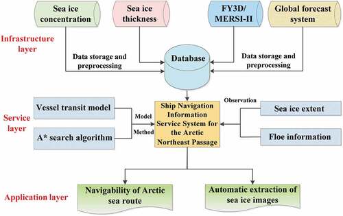
The infrastructure layer developed based on the Big Data and Cloud Service Platform (BDCSP, http://english.casearth.com) provides the scalable hardware and software environment where our system runs. All data storage and processing in the SNISS are completed in this layer.

The service layer consists of a series of web services running on a computer, which is key to realizing the analysis required for ship navigation, including the realization of some key algorithms, such as the vessel transit model and A* search algorithm.

The application layer provides the main functions of our system, such as route analysis using 3D GIS and automatic sea ice image extraction, which are realized based on the secondary development engine (DESP Client for WebGL), a digital Earth foundation platform provided by the Aerospace Information Research Institute, CAS. The main technology used by this engine is described in Table 2.

Table 2. Main technologies of the secondary development engine.

Function	Description of the main technology	Link
User interaction	Vue: Open source front-end framework	https://vuejs.org/index.html
	iView: Vue-based open source user interface (UI) component library	http://iview.talkingdata.com/
	Cesium: Open source 3D JavaScript (JS) library	https://cesium.com/cesiumjs/
	Echarts D3: Open source chart library	http://echarts.apache.org/
Data exchange	Apache Tomcat: Open source implementation of the Java Servlet, JavaServer Pages, Java Expression Language and Java WebSocket technologies	https://tomcat.apache.org/
	Redis: Data buffer container	https://redis.io/
	GeoServer: Image publishing service	http://geoserver.org/

4. Study area and data

In this section, the study area and detailed data processing are presented. The latter includes the sea ice data processing method and true-colour image composite method for Fengyun-3D.

4.1. Study area

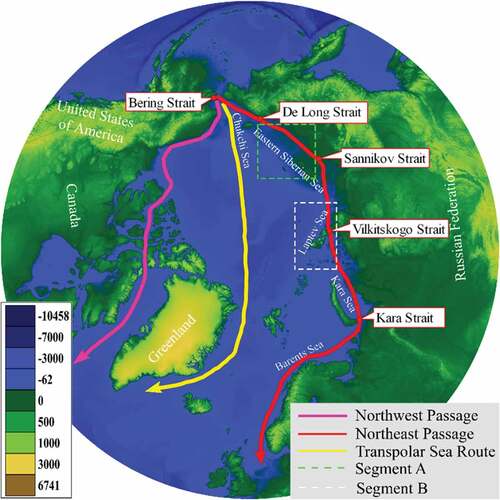
The focus of this study is the NEP (Figure 2), which starts from Northeast Asia, crosses westward across the Pacific Ocean, and passes through the Chukchi Sea, Eastern Siberian Sea, Laptev Sea, Kara Sea, Barents Sea, and Norwegian Sea in the southern part of the Arctic Ocean (Byers, & Lodge, 2019; Song et al., 2019). This route is the shortest channel connecting Asia, Europe, and North America. The key waters affecting the navigation of the route are the following (Ma et al., 2019):

1. From the middle of the Eastern Siberian Sea to the west along the NEP to the Sannikov Strait (defined as segment A, the geographic centre coordinates are 72.7°N, 159.8°E);

2. From the central part of the Laptev Sea (120°E) to the west along the channel, it passes through the Velikitsky Strait to the waters of the Kara Sea (defined as segment B, the central geographic coordinates are 77.9°N, 105.9°E).

Figure 2. The distribution of Arctic routes.

4.2. Data acquisition and preparation

4.2.1. Sea ice data processing method

The sea ice thickness and concentration are critical factors for analysing accessibility along the NEP. In this study, the sea ice concentration values from 2012 to 2020 were downloaded from the National Snow and Ice Data Center (NSIDC), and the sea ice thickness values from 2012 to 2020 were collected from the Pan-Arctic Ice-Ocean Modelling and Assimilation System (PIOMAS). Meanwhile, sea ice concentration and thickness from May to September 2021 (updated daily and nowcasting 60 days) were automatically downloaded from the Laboratory of Atmospheric Sciences and Geophysical Fluid Dynamics (LASG), Institute of Atmospheric Physics (IAP), CAS. Once these data are updated, our system will automatically calculate the latest route prediction results. In addition, climate projections of the sea ice conditions were obtained from the C3S Global Shipping service (Table 3). The reasons why we chose only these four datasets in this project are because these data have the following important characteristics:

Table 3. Main data used in this study (the information in this table was updated on August 1, 2021).

No.	Variable	Source	Format	Time	Period	Resolution	Link
1	Sea ice concentration	MASIE-AMSR2	NetCDF	2012 to present	day	4 km	https://nsidc.org/data/G10005/versions/1
		IAP LASG	NetCDF	May 2021 to October 2021	day	1°	http://project.lasg.ac.cn/FGOALS_f2-S2S/index.php
		C3S Global Shipping service	NetCDF	2010 to 2100	month	1°	https://cds.climate.copernicus.eu/cdsapp#!/dataset/sis-shipping-arctic?tab=overview
2	Sea ice thickness	PIOMAS model	NetCDF	1978 to present	day	0.1–2.5°	http://psc.apl.uw.edu/research/projects/arctic-sea-ice-volume-anomaly/data/model_grid
		IAP LASG	NetCDF	May 2021 to October 2021	day	1°	http://project.lasg.ac.cn/FGOALS_f2-S2S/index.php
		C3S Global Shipping service	NetCDF	2010 to 2100	month	1°	https://cds.climate.copernicus.eu/cdsapp#!/dataset/sis-shipping-arctic?tab=overview

(1) Data are gridded, which is convenient to calculate the risk value of each grid.

(2) The dataset is a long time series, including historical and future data, and the data are updated in real time.

(3) Data can be easily downloaded through our background program.

(4) Data are available during the melting season (July to September).

In fact, our system provides a flexible data processing interface, which can flexibly use different data sources for automatic download and preprocessing. If there are more suitable data in the later period, we can quickly replace the data sources. However, some key problems need to be solved when these data are applied to route planning. These data are all irregular grid data in NetCDF format, which means that the grid is dense near the North Pole and relatively sparse near the equator. This type of data cannot be displayed in a 3D GIS platform such as Cesium. In addition, when the navigation risk is calculated from the sea ice concentration and thickness data, these two irregular grids are quite different in resolution and number of grid points, which cannot meet the needs of matrix operations. Therefore, the data need to be preprocessed before they can be analysed and displayed. There are three main pre-processing steps.

Step 1: Construction of a regular grid

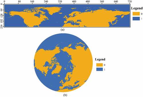
A regular grid is constructed to convert the data from different irregular grids into a unified format, which is convenient for data analysis and calculation. As shown in Figure 3(a), we constructed a 256-row by 720-column grid (longitude range: 180°W–180°E, latitude range: 26°N–90°N) based on the sea ice concentration and thickness data coverage; the grid points of the regular grid were classified into land (zero) and sea (one), which reduced the calculation time by limiting the calculation process to marine areas (grid points that were assigned a value of one).

Figure 3. Regular grids with different projections (blue represents oceans, and yellow represents land). (a) Regular grid (WGS 1984 World Mercator). (b) Regular grid (North Pole Orthographic).

Step 2: Storage of irregular grid data

The spatial information and variable values corresponding to each grid point of the irregular grid are saved in a spatial database to prepare for the assignment to the regular grid. Taking sea ice concentration data as an example, the irregular grid data include 1,970,874 grid points, each containing multiple attributes, such as longitude, latitude, and sea ice concentration. This information can be stored in a spatial database (PostGIS) with geometric objects (geometry).

Step 3: Assignment of a regular grid

The longitude and latitude of each grid point are obtained by traversing each grid object in the regular grid (considering only marine grid points that have been assigned a value of one). The target point closest to this longitude and latitude is then queried in the spatial database, and the value of this target point is assigned to the grid point of the regular grid. When the traverse is complete, each grid point in the regular grid has information on the values of variables such as sea ice concentration. The SQL statement used to realize this process is as follows:

“select ST_distance (geom:: geography, GeomFromEWKT (“SRID = 4326; POINT (“ + lon + “ “ + lat + “ 10)”):: geography) distance, t. * from “ + tb_name + “ where ST_dwithin (geom::geography, GeomFromEWKT (‘SRID = 4326; POINT (“ + lon + “ “ + lat + “ 10)’):: geography, 2500000) order By distance limit 1”;

where lon and lat represent the longitude and latitude of the regular grid point, respectively; distance represents the size of the search range when searching for discrete points through the latitude and longitude information of the grid point; and tb_name represents the name of the data table storing the discrete irregular points.

After the above three steps, the generation of regular grid data is realized, and the data can be used for real-time calculation of the optimal route and data visualization in Cesium.

4.2.2. True-colour image composite method for Fengyun-3D

The data from the Medium Resolution Spectrum Imager-II (MERSI-II) onboard Fengyun-3D (FY-3D) are utilized to generate true-colour sea ice images after radiation calibration in this study (http://www.nsmc.org.cn/en/NSMC/Home/Index.html). Table 3 shows the main bands of FY-3D/MERSI-II used in this work. The sea ice images are extracted using 1 to 3 bands of land and cloud boundary characteristics after FY-3D/MERSI-II radiation calibration. The main steps include radiation calibration, geometric correction, band combination, projection and cropping, and data format conversion.

(1) Radiation calibration

Through calibration by Equation 1(1) ${\rho }_{\lambda }=\frac{K_0+K_1\times DN+K_2\times \left(D{N^{\ast }}^2\right)}{cos\theta }$(1) , the digital number (DN) value in the image is converted into top of atmosphere (TOA) reflectance. Before calibration, all channel data have to be adjusted and restored by the DN value (Equation 2(2) $D{N}^{\ast }=slope\times \left(DN-intercept\right)$(2) ), and the slope and intercept parameters in the formula are obtained from the header file.

(1) ${\rho }_{\lambda }=\frac{K_0+K_1\times DN+K_2\times \left(D{N^{\ast }}^2\right)}{cos\theta }$(1)

(2) $D{N}^{\ast }=slope\times \left(DN-intercept\right)$(2)

where ρ_λ is the TOA reflectance; K₀, K₁, and K₂ are calibration coefficients; θ is the solar zenith angle; and slope and intercept are the internal attributes of the corresponding dataset.

(2) Geometric correction

The FY-3D/MERSI-II image header file provides the geographic location information of each initial pixel in the form of latitude and longitude, so the original data are geometrically corrected by the geographic lookup table (GLT) method with high correction accuracy.

(3) Band combination

The FY-3D/MERSI-II has five 250-m and fifteen 1-km spatial resolution bands (Table 4), and the scan width exceeds 2,000 km. In this study, the first three bands (650, 550 and 470 nm) are used to synthesize a true-colour sea ice image, where bright white is snow; white can be clouds, sea ice, or melting snow; cyan is mostly melting ice on surface snow; grey is mainly ice clouds or thin water clouds; dark green is land; and black is water.

Table 4. Main three bands of FY-3D/MERSI-II used in this work and its application and physical parameters.

P	Band	R (μm)	L (nm)	S (m)	N (ΔT~K)	M (ρ, K)
Remote sensing of land andcloud boundaries and their characteristics	1	0.470	50	250	100	90%
	2	0.550	50	250	100	90%
	3	0.650	50	250	100	90%

P indicates the primary purpose of each band, Band represents the band number, R represents the centre wavelength, L represents the spectral bandwidth, S represents the spatial resolution, N represents the signal-to-noise ratio or noise equivalent temperature difference, M represents the dynamic range, ρ is the unit of reflectivity, and K is the unit of brightness temperature.

(4) Projection and cropping

The WGS 1984 projection data are automatically converted to Lambert azimuthal equal area projection data using the open source library PROJ (https://proj.org/) and cropped to the projected image based on parameters set by the user (the default width is 1,600 × 1,600 pixels).

(5) Data format conversion

After the above steps, the sea ice optical image of the area set by the user is obtained, but its data format is HDF, which cannot be directly used in 3D GIS such as Cesium. It needs to be converted into JPG, and the conversion process can be downloaded from this link (https://github.com/ypf19940828/wad20200223).

5. SNISS algorithms

This section introduces two important algorithms used for ship navigation analysis.

5.1. Vessel transit model

The International Maritime Organization (IMO) developed a harmonized methodology for assessing operational limitations in ice navigation called the Polar Operational Limit Assessment Risk Indexing System (POLARIS) in 2016 (Bai, 2015; Stoddard et al., 2017). POLARIS provides a risk assessment framework to assess navigational safety in icy conditions, which is similar to the ice multiplier of the ATAM from the Arctic Ice Regime Shipping System (Howell & Yackel, 2014; Stephenson, Smith, & Agnew, 2011).

POLARIS assesses ice conditions based on the risk index outcome (RIO) determined by the following calculation:

(3) $RIO=(C_1\times R{V}_1)+(C_2\times R{V}_2)+(C_3\times R{V}_3)+\dots +(C_n\times R{V}_n)$(3)

where C₁ … C_n represent the concentrations of ice types within the ice regime, and RV₁ … RV_n represent the corresponding risk index values (RV) for a given ice class. The subscripts of C_n and RV_n represent the number in the calculation grid area (the value of n is 184,320 in this study, which is determined by the row and column numbers of the defined grid). Details are provided in section 4.2.1). POLARIS provides RV for the seven International Association of Classification Societies (IACS) polar classes, four Finnish-Swedish ice classes, and non-ice-class ships. There are 12 types of sea ice in the POLARIS system. For a specific ship type, its RV in a certain type of sea ice area can be obtained by the POLARIS lookup table (Bai, 2015). Taking an ordinary merchant ship as an example, the RV can be obtained from the lookup table (Equation 4(4) $\mathrm{R}{\mathrm{V}}_{\mathrm{T}}=\left\{\begin{array}{ccc}3& \mathrm{T}=0& \mathrm{I}\mathrm{c}\mathrm{e}\mathrm{f}\mathrm{r}\mathrm{e}\mathrm{e}\\ 1& 0\mathrm{m}<\mathrm{T}<0.10\mathrm{m}& \mathrm{N}\mathrm{e}\mathrm{w}\mathrm{i}\mathrm{c}\mathrm{e}\\ 0& 0.10\mathrm{m}\le \mathrm{T}<0.15\mathrm{m}& \mathrm{G}\mathrm{r}\mathrm{e}\mathrm{y}\mathrm{i}\mathrm{c}\mathrm{e}\\ -1& 0.15\mathrm{m}\le \mathrm{T}<0.30\mathrm{m}& \mathrm{G}\mathrm{r}\mathrm{e}\mathrm{y}\mathrm{w}\mathrm{h}\mathrm{i}\mathrm{t}\mathrm{e}\mathrm{i}\mathrm{c}\mathrm{e}\\ -2& 0.30\mathrm{m}\le \mathrm{T}<0.50\mathrm{m}& \mathrm{T}\mathrm{h}\mathrm{i}\mathrm{n}{1}^{\mathrm{s}\mathrm{t}}\mathrm{y}\mathrm{e}\mathrm{a}\mathrm{r}\mathrm{i}\mathrm{c}\mathrm{e}{1}^{\mathrm{s}\mathrm{t}}\mathrm{s}\mathrm{t}\mathrm{a}\mathrm{g}\mathrm{e}\\ -3& 0.50\mathrm{m}\le \mathrm{T}<0.70\mathrm{m}& \mathrm{T}\mathrm{h}\mathrm{i}\mathrm{n}{1}^{\mathrm{s}\mathrm{t}}\mathrm{y}\mathrm{e}\mathrm{a}\mathrm{r}\mathrm{i}\mathrm{c}\mathrm{e}{2}^{\mathrm{s}\mathrm{t}}\mathrm{s}\mathrm{t}\mathrm{a}\mathrm{g}\mathrm{e}\\ -3& 0.70\mathrm{m}\le \mathrm{T}<0.95\mathrm{m}& \mathrm{M}\mathrm{e}\mathrm{d}\mathrm{i}\mathrm{u}\mathrm{m}{1}^{\mathrm{s}\mathrm{t}}\mathrm{y}\mathrm{e}\mathrm{a}\mathrm{r}\mathrm{i}\mathrm{c}\mathrm{e}{1}^{\mathrm{s}\mathrm{t}}\mathrm{s}\mathrm{t}\mathrm{a}\mathrm{g}\mathrm{e}\\ -3& 0.95\mathrm{m}\le \mathrm{T}<1.20\mathrm{m}& \mathrm{M}\mathrm{e}\mathrm{d}\mathrm{i}\mathrm{u}\mathrm{m}{1}^{\mathrm{s}\mathrm{t}}\mathrm{y}\mathrm{e}\mathrm{a}\mathrm{r}\mathrm{i}\mathrm{c}\mathrm{e}{2}^{\mathrm{s}\mathrm{t}}\mathrm{s}\mathrm{t}\mathrm{a}\mathrm{g}\mathrm{e}\\ -4& 1.20\mathrm{m}\le \mathrm{T}<2.00\mathrm{m}& \mathrm{T}\mathrm{h}\mathrm{i}\mathrm{c}\mathrm{k}{1}^{\mathrm{s}\mathrm{t}}\mathrm{y}\mathrm{e}\mathrm{a}\mathrm{r}\mathrm{i}\mathrm{c}\mathrm{e}\\ -5& 1.20\mathrm{m}\le \mathrm{T}<2.00\mathrm{m}& \mathrm{S}\mathrm{e}\mathrm{c}\mathrm{o}\mathrm{n}\mathrm{d}\mathrm{y}\mathrm{e}\mathrm{a}\mathrm{r}\mathrm{i}\mathrm{c}\mathrm{e}\\ -6& 2.00\mathrm{m}\le \mathrm{T}<3.00\mathrm{m}& \mathrm{L}\mathrm{i}\mathrm{g}\mathrm{h}\mathrm{t}\mathrm{m}\mathrm{u}\mathrm{l}\mathrm{t}{\mathrm{i}}_{{ }^{-}}\mathrm{y}\mathrm{e}\mathrm{a}\mathrm{r}\mathrm{i}\mathrm{c}\mathrm{e}\\ -6& 3.00\mathrm{m}\le \mathrm{T}& \mathrm{H}\mathrm{e}\mathrm{a}\mathrm{v}\mathrm{y}\mathrm{m}\mathrm{u}\mathrm{l}\mathrm{t}{\mathrm{i}}_{{ }^{-}}\mathrm{y}\mathrm{e}\mathrm{a}\mathrm{r}\mathrm{i}\mathrm{c}\mathrm{e}\end{array}\right.$(4) ). RV ranges from −6 to +3, and its value indicates the risk level of a specific ship when sailing in an area covered by a certain sea ice type.

(4) $\mathrm{R}{\mathrm{V}}_{\mathrm{T}}=\left\{\begin{array}{ccc}3& \mathrm{T}=0& \mathrm{I}\mathrm{c}\mathrm{e}\mathrm{f}\mathrm{r}\mathrm{e}\mathrm{e}\\ 1& 0\mathrm{m}<\mathrm{T}<0.10\mathrm{m}& \mathrm{N}\mathrm{e}\mathrm{w}\mathrm{i}\mathrm{c}\mathrm{e}\\ 0& 0.10\mathrm{m}\le \mathrm{T}<0.15\mathrm{m}& \mathrm{G}\mathrm{r}\mathrm{e}\mathrm{y}\mathrm{i}\mathrm{c}\mathrm{e}\\ -1& 0.15\mathrm{m}\le \mathrm{T}<0.30\mathrm{m}& \mathrm{G}\mathrm{r}\mathrm{e}\mathrm{y}\mathrm{w}\mathrm{h}\mathrm{i}\mathrm{t}\mathrm{e}\mathrm{i}\mathrm{c}\mathrm{e}\\ -2& 0.30\mathrm{m}\le \mathrm{T}<0.50\mathrm{m}& \mathrm{T}\mathrm{h}\mathrm{i}\mathrm{n}{1}^{\mathrm{s}\mathrm{t}}\mathrm{y}\mathrm{e}\mathrm{a}\mathrm{r}\mathrm{i}\mathrm{c}\mathrm{e}{1}^{\mathrm{s}\mathrm{t}}\mathrm{s}\mathrm{t}\mathrm{a}\mathrm{g}\mathrm{e}\\ -3& 0.50\mathrm{m}\le \mathrm{T}<0.70\mathrm{m}& \mathrm{T}\mathrm{h}\mathrm{i}\mathrm{n}{1}^{\mathrm{s}\mathrm{t}}\mathrm{y}\mathrm{e}\mathrm{a}\mathrm{r}\mathrm{i}\mathrm{c}\mathrm{e}{2}^{\mathrm{s}\mathrm{t}}\mathrm{s}\mathrm{t}\mathrm{a}\mathrm{g}\mathrm{e}\\ -3& 0.70\mathrm{m}\le \mathrm{T}<0.95\mathrm{m}& \mathrm{M}\mathrm{e}\mathrm{d}\mathrm{i}\mathrm{u}\mathrm{m}{1}^{\mathrm{s}\mathrm{t}}\mathrm{y}\mathrm{e}\mathrm{a}\mathrm{r}\mathrm{i}\mathrm{c}\mathrm{e}{1}^{\mathrm{s}\mathrm{t}}\mathrm{s}\mathrm{t}\mathrm{a}\mathrm{g}\mathrm{e}\\ -3& 0.95\mathrm{m}\le \mathrm{T}<1.20\mathrm{m}& \mathrm{M}\mathrm{e}\mathrm{d}\mathrm{i}\mathrm{u}\mathrm{m}{1}^{\mathrm{s}\mathrm{t}}\mathrm{y}\mathrm{e}\mathrm{a}\mathrm{r}\mathrm{i}\mathrm{c}\mathrm{e}{2}^{\mathrm{s}\mathrm{t}}\mathrm{s}\mathrm{t}\mathrm{a}\mathrm{g}\mathrm{e}\\ -4& 1.20\mathrm{m}\le \mathrm{T}<2.00\mathrm{m}& \mathrm{T}\mathrm{h}\mathrm{i}\mathrm{c}\mathrm{k}{1}^{\mathrm{s}\mathrm{t}}\mathrm{y}\mathrm{e}\mathrm{a}\mathrm{r}\mathrm{i}\mathrm{c}\mathrm{e}\\ -5& 1.20\mathrm{m}\le \mathrm{T}<2.00\mathrm{m}& \mathrm{S}\mathrm{e}\mathrm{c}\mathrm{o}\mathrm{n}\mathrm{d}\mathrm{y}\mathrm{e}\mathrm{a}\mathrm{r}\mathrm{i}\mathrm{c}\mathrm{e}\\ -6& 2.00\mathrm{m}\le \mathrm{T}<3.00\mathrm{m}& \mathrm{L}\mathrm{i}\mathrm{g}\mathrm{h}\mathrm{t}\mathrm{m}\mathrm{u}\mathrm{l}\mathrm{t}{\mathrm{i}}_{{ }^{-}}\mathrm{y}\mathrm{e}\mathrm{a}\mathrm{r}\mathrm{i}\mathrm{c}\mathrm{e}\\ -6& 3.00\mathrm{m}\le \mathrm{T}& \mathrm{H}\mathrm{e}\mathrm{a}\mathrm{v}\mathrm{y}\mathrm{m}\mathrm{u}\mathrm{l}\mathrm{t}{\mathrm{i}}_{{ }^{-}}\mathrm{y}\mathrm{e}\mathrm{a}\mathrm{r}\mathrm{i}\mathrm{c}\mathrm{e}\end{array}\right.$(4)

One example application of the calculation of the RIO based on POLARIS is presented in Figure 4. This map makes use of historical sea ice concentration from NSIDC and sea ice thickness from PIOMAS to compute the RIO for a merchant ship navigating in the Arctic. A positive RIO indicates an acceptable risk level where a type of ship can sail, while a negative RIO indicates an increased risk level for the same type of ship. In addition to the meteorological conditions, the RIO represents one of the important bases of our system to evaluate whether a ship can safely sail in a certain area.

Figure 4. Spatial distribution of the risk index outcome (RIO) for a merchant ship on October 15, 2019.

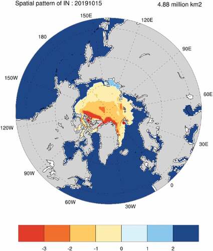
Compared with the Canadian Arctic Ice Regime Shipping System (AIRSS), POLARIS of the IMO incorporates a more comprehensive ship class type list, identifies different sea ice types, and further refines the risk quantification levels. These improvements not only contribute to the international application of this risk assessment scheme but also allow more detailed and accurate navigation risk assessments for specific ice conditions.

5.2. A* search algorithm

The Arctic’s sea ice and weather are constantly changing, but for a specific time (data in the Arctic region are usually updated according to a fixed cycle, e.g. 6 hours, one day), these variables can be described by a static grid (256 rows by 720 columns), where each grid point provides information on the locations’ RIO, weather, and terrain. Therefore, if the locations of the start and end points are determined, an optimal navigation path can be calculated using the A* algorithm (Zeng & Church, 2009), which is the most effective direct search method for identifying the shortest path in a static road network (Wang, Zhang, & Qian, 2018).

Specifically, A* selects the path that minimizes f(n):

(5) $f\left(n\right)=g\left(n\right)+h\left(n\right)$(5)

where n is the next node on the path, g(n) is the cost of the path from the start node to n, and h(n) is a heuristic function that estimates the cost of the path from n to the destination. In this study, we assume that the lower the cost, the higher the score, based on comprehensive factors such as distance, RIO, and meteorological variables such as visibility, wind speed, and temperature; the score determines the priority with which routes should be selected. Therefore, the problem that needs to be solved is finding the optimal navigation direction out of eight different possible directions according to a score evaluation. When we choose the next node to traverse, we choose the node with the highest overall priority (highest score). The score calculation uses the following strategy:

(1) Based on the principle of the shortest distance, the score of the adjacent node is increased if it is farther from the starting point (score+ = 10), and the score of the adjacent node is decreased if it is closer to the end point (score+ = 10). This strategy ensures that routes is constantly approaching the destination.

(2) Routes can only be distributed over the ocean, so the score of an adjacent node is increased (score+ = 10) if it is located over the ocean or reduced (score+ = −9999, meaning that the ships cannot pass through the area) if it is located over land.

(3) Only the shortest path may not be enough for the sake of safety. As mentioned by Liu, Sattar, and Li (2016), routes should be as far away from sea ice as possible. Therefore, RIO values are also utilized to quantitatively analyze optimal routes in our algorithm. Namely, if the RIO value of the adjacent node is positive, the score for that node is increased (score+ = 10), while if the RIO value is negative, the score is reduced (score+ = −9999). This strategy ensures that routes can only be distributed in areas where RIO is positive, ensuring the safety of ships.

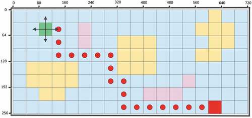
According to the above strategies, the SNISS can automatically calculate the optimal daily route along the NEP for different ships in the period of the navigation. As shown in Figure 5, the track composed of red dots illustrated the best route for navigation, which are displayed over gridded data with 256 rows and 720 columns. Obviously, the optimal route calculated by our algorithm is the result of automatically searching the shortest path in the safe navigation areas.

Figure 5. Optimal route extraction results. The coordinates in the figure represent the row and column numbers of the data; the green grid is the starting point and the red grid is the end point; yellow grids represent lands, light blue grids represent regions with positive RIO and pink ones represents regions with negative RIO.

6. SNISS examples

In this section, the two most important functionalities of the SNISS are presented together with two scenarios. They are route analyses using 3D GIS and automatic sea ice image extraction and provide important reference information for ship navigation from the macroscale to local perspective.

6.1. Route analysis using 3D GIS

The SNISS calculates the distribution of the optimal route for ordinary merchant ships with no ice breaking abilities and Ice Class PC1 ships that are designed for operation in at least medium first-year ice (i.e. nominal ice thickness > 70 cm) during the navigation period of the NEP from the past 10 years to the next 100 years. It also provides information on sea ice changes along the route and can obtain temperature changes in local areas for the next 10 days.

(1) Display the optimal navigation route in 3D GIS

The system automatically downloads sea ice data every day and converts irregular grid data to regular grid data. On this basis, the system calculates the distribution of the Arctic navigation RIO, automatically extracts the optimal route based on the A* algorithm and records the latitude and longitude of each point of the navigation path to generate vector route data (such as in GeoJSON format). Then, these vector route data are published as a web map service (WMS) on the GeoServer and displayed in the Cesium 3D visualization platform. In our system, the navigation routes with three different time periods are automatically calculated, including ship accessibility for historical conditions (July 2012 to October 2020), short-term forecasts (May to September 2021, updated data for the next 60 days every day), and future projections (July 2022 to October 2100).

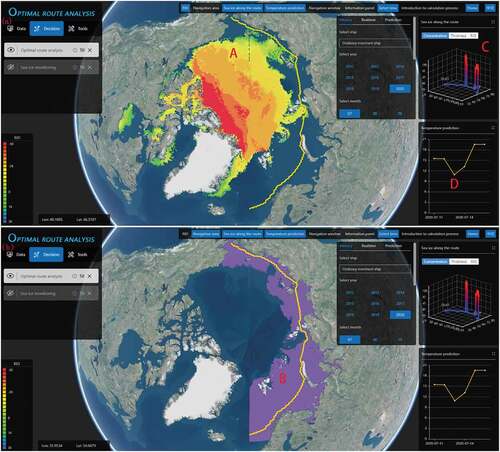
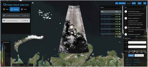
The first scenario (Figure 6) provides an example of merchant ship sailing in the NEP to shows an optimal route calculated by the system on July 15, 2020 (yellow line). Yellow, orange and red areas in Figure 6(a) indicate higher risk levels (RIO<0) for merchant ships, while merchant ships are able to safely navigate in green or blue areas (RIO>0). In order to guide the navigation of ships more conveniently, we further define the regions where RIO is greater than zero as buffer zones (purple areas in Figure 6(b)), where ships can navigate safely.

Figure 6. Optimal route analysis interface (http://arcticroute.tpdc.ac.cn/encesium_index/?type=1&locale=en). Users can select the date for which the distribution of the optimal route is displayed. In figure (a), A: the yellow line on the map is the optimal route calculated by the system for merchant ships sailing in the NEP on July 15, 2020; the map colours represent the RIO for merchant ships on this day. C: visualization of sea ice concentration and thickness along the NEP. D: ten- to fifteen-day temperature forecast along the optimal route. In figure (b), B: the buffer zone where ships can navigate safely.

(2) Display sea ice changes along the route in 3D GIS

The optimal route is composed of a series of vector points. Therefore, according to the longitude and latitude coordinates of these points, the corresponding sea ice concentration and sea ice thickness values of the points can be queried from the spatial database. On this basis, we display the changes in sea ice concentration and thickness along the NEP using a 3D chart, which helps guide ship navigation (Figure 6(c)).

(3) Display meteorological information along the route in 3D GIS

Based on the Global Forecast System (GFS), SNISS provides predictions of local meteorological conditions along the route for the next 10–15 days, which serve as an important reference for ship navigation. For example, the temperature forecast for the next 10–15 days can be retrieved by clicking on the route and its adjacent areas in 3D GIS (Figure 6(d)).

6.2. Automatic sea ice image extraction

The navigation analysis module discussed in the previous section quantitatively analyses the navigation risk of the Arctic waterway from a macroscale perspective. For key local sea straits, SNISS can perform online real-time analyses of sea ice images based on FY-3D (Figure 7). This function can provide accurate and real-time information services for the navigation of Arctic ships. Therefore, it is a further supplement to the route distribution information (low resolution) and its implementation steps are as follows.

Figure 7. Automatic extraction process of sea ice image.

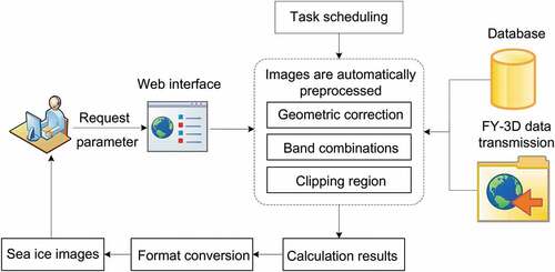
1. Region selection

In traditional data sharing platforms, a research area is usually selected by filling in an online form or drawing a rectangle on a 2D map, which is not user-friendly. In this study, regions of interest can be intuitively selected on the spherical system to obtain its range of longitude and latitude.

(2)  Parameter passing

The system passes calculation parameters through an HTTP request as follows:

“http://210.*.*.49:8080/done/Action?longitude=80&dimensionality=93&userId=5&userName=kaka&[email protected]”.

Through this request, some parameters, such as the latitude and longitude of the centre of the region of interest, user ID, user name, and user email, are sent to the web service interface.

(3)  Calling the web service

The web service for remote sensing image extraction is deployed on three servers (the extraction can be calculated by three users at the same time and can be expanded to multiple servers). In this way, each user’s request is allocated according to the response time of these three web services, and web services with short response times are preferentially allocated to users for online calculations. The function of the web service is to seamlessly combine different programs to realize the automatic extraction of sea ice images (for more details, refer to section 3.2.1).

(4)  Results display

According to the conditions input by users and the calculations of the above steps in the SNISS, the true-colour image results of sea ice in this area are automatically extracted and displayed in 3D GIS. The system supports local zoom-in and zoom-out functions and displays the longitude and latitude of the cursor position, which allows users to clearly visualize the distribution and shape of sea ice in this area.

The second scenario shows how to obtain sea ice images in real time from the SNISS in the Vilkitskogo Strait (Figure 8). After the calculation command is submitted, our system begins the online real-time calculations for the true-colour image of sea ice (the data time is July 15, 2020), and the calculation progress can be viewed through the time progress in the lower right corner. Generally, the calculation time of each scene image is 3–4 minutes. Once this calculation is completed, our system automatically sends an email to inform the user how to obtain and use the calculation results. Meanwhile, the calculation result is displayed in 3D GIS (Figure 9), which can help navigator determine the ice conditions in local areas and make reasonable decisions (higher resolution).

Figure 8. Drawing a rectangle to select a region of interest (http://arcticroute.tpdc.ac.cn/encesium_index/?type=2&locale=en).

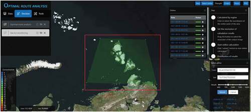
Figure 9. The online calculation results are automatically displayed in the spherical system.

7. Discussion

The above experiments demonstrated that the use of the DESP Client for WebGL and the automated workflow are both effective and feasible for ship navigation analysis and visualization. Compared with other available 3D GIS toolkits, the SNISS is designed as a browser-server (BS) tiered architecture based on the DESP Client for WebGL; therefore, the software applications are hosted by service providers and made available to users via the internet. More specifically, the visualization framework based on the DESP Client for WebGL enables users to achieve a fast interaction, such as rotation, zooming, panning, and enquiries, of calculation results related to ARs. In addition, the automated data processing in the SNISS, which is deployed in BDCSP, simplifies the daily workflow of tedious model processing tasks and significantly improves computing efficiency. In Table 5, we compared the SNISS with a route planning system using Google Earth (Chang, He, Chou, Kao, & Chiou, 2015). Our newly built system has obvious advantages in automation. Moreover, all the adopted technologies in the SNISS are open-source, and none of the software or plug-ins need to be installed on a client-side computer because of its BS architecture.

Table 5. Comparison between SNISS and route planning system using Google Earth.

Name	Main functionalities	Area	3D GIS platform	Factors to be considered for route planning	Calculation method	Other auxiliary functionalities
Route planning system using Google Earth	Route planning for major ports between Asia and Europe	NEP	Google Earth	Distribution of the Arctic floating ice areas, water depth	Manual analysis and processing	Comparing the NEP with the traditional route through the Suez Canal using a dynamic analysis of the cost efficiency
SNISS	Route analyses and automatic sea ice image extraction	NEP	Caesium	Sea ice concentration and thickness, distance	Automatic completion	Changes in sea ice concentration and thickness along the NEP are presented using a 3D chart

Although the SNISS based on BS architecture has many visual advantages compared with traditional client-server (CS) architecture systems, we do not claim that this 3D GIS-based system can completely replace existing standalone visualization toolkits. In contrast, this paper only demonstrates that a combination of a 3D GIS framework and online computing workflow is feasible and scalable for ship navigation analysis. In particular, the analytical methods and available data in the SNISS can be easily expanded or replaced according to the requirements. For example, the A* algorithm used in the SNISS has been proven to be an effective and accurate method for route analysis application scenarios, but this does not mean it is the only effective method in the CASEarth Poles platform. In fact, other methods, such as reinforcement learning (Mnih et al., 2015) and Dijkstra (Deng, Chen, Zhang, & Mahadevan, 2012; Zhu & Sun, 2021), have also shown good application potential in route analysis. Therefore, our system provides a flexible algorithm interface for the methods library in the CASEarth Poles platform. For the validation of the methods and results, our future work will be conducted as long as we have access to real navigation data. At the same time, the SNISS currently uses only FY-3D data to automatically extract local sea ice information, showing that the entire processing flow is very effective and accurate. However, other remote sensing data from the Chinese HY-1 C satellite, Sentinel-1 synthetic aperture radar or Advanced Microwave Scanning Radiometer 2 passive microwave radiometer, among others, are also appropriate for the automatic processing framework proposed in this study. In this case, we considered the scalability of these data at the beginning of the system design for framework and function. To include new datasets, developers need to only choose different methods for different data, with no need to modify the system architecture and processing flow. Because of these flexible expansion strategies for methods and data in our system, it is easily adapted to other applications.

Despite its several advances, the SNISS also has certain limitations. First, only factors such as distance, sea ice condition and terrain are considered when calculating the optimal navigation channel, and meteorological factors such as temperature, snowfall, and wind speed still need to be added so that ships can bypass areas with bad weather. In addition, the system only provides navigation path analysis for ordinary merchant ships and Ice Class PC1 ships, and the optimal path analysis of icebreakers of different levels still needs to be included. Finally, we cannot download all of the FY-3D data for the Arctic to our server due to the large data volume. Therefore, at present, our strategy is to download FY-3D data according to the navigation requirements (setting the strait range and time). On the basis of obtaining the original data, our system can process and visualize these original data in real time (according to the conditions of regional scope and time). Although the remote sensing images of sea ice calculated by the system in real time can show the location and size of ice floes, they cannot be used to quantitatively calculate sea ice parameters, such as sea ice extent and type. These parameters need to be extracted based on deep learning approaches.

8. Conclusion

In this study, we developed an advanced navigation information service system for the Arctic Northeast Passage (NEP) using a 3D GIS platform. First, according to the characteristics of Arctic multisource data, we selected typical and important sea ice and meteorological data and constructed an automatic data processing workflow. Based on the data processing, we developed an intelligent method for extracting the optimal Arctic route based on a heuristic search algorithm, which provides navigation guidance for ships from a macroscale perspective. For local sea areas of concern to users, we built a more efficient real-time sea ice image extraction system based on a cloud platform, which provides important reference information for ship navigation. Finally, we integrated these data and methods into the 3D GIS system and established a navigation information service system for the NEP, which is currently running in the BEDCSP and can be accessed and used at various terminals (http://arcticroute.tpdc.ac.cn/encesium_index/?type=1&locale=en), such as the ball screen system and arc screen system in the 2D exhibition hall of the National Science Library, Chinese Academy of Sciences, and can also be accessed from notebook computers, iPads, and mobile phones. This navigation information service system for the NEP provides accurate information about channel distribution, meteorology, and local sea ice for Arctic merchant ships and has important significance for building the Polar Silk Road.

Acknowledgments

Since its implementation in 2019, the construction of the SNISS has been aided by the Aerospace Information Research Institute, Chinese Academy of Sciences; Institute of Atmospheric Physics, Chinese Academy of Sciences; Computer Network Information Center, Chinese Academy of Sciences; National Satellite Meteorological Centre; and China Meteorological Administration. We would like to express sincere appreciation to them for their work in network platform development, data service, and system running environment. We are also grateful to the editor and the anonymous reviewers for their valuable comments and suggestions, which have improved the presentation of the manuscript.

Disclosure statement

No potential conflict of interest was reported by the author(s).

Data availability statement

Data are openly available in a public repository that does not issue DOIs. The sea ice concentration data from 2012 to present are openly available at https://nsidc.org/data/G10005/versions/1, and the sea ice thickness data from 2012 to present are openly available at http://psc.apl.uw.edu/research/projects/arctic-sea-ice-volume-anomaly/data/model_grid. In addition, climate projections of the sea ice conditions are openly available at https://cds.climate.copernicus.eu/cdsapp#!/dataset/sis-shipping-arctic?tab=overview.

Additional information

Funding

This project is supported by the “CAS Big Earth Data Science Engineering (CASEarth)” program, and a Strategic Priority Research Program of the Chinese Academy of Sciences [Grant XDA19070100].

Notes on contributors

Adan Wu

Adan Wu is currently pursuing a Ph.D. degree from the Northwest Institute of Eco-Environment and Resources, Chinese Academy of Sciences, University of Chinese Academy of Sciences, Beijing, China. His research interests include the Internet of Things, smart information services and big data analysis. He has developed several information systems, such as a web-based visualization system for a wireless sensor network in the Heihe Watershed Allied Telemetry Experimental Research project, a decision-making system for preventing and forecasting disasters in the Qinghai-Tibet permafrost engineering corridor and an information service system for the Northeast Passage in the Arctic.

Tao Che

Tao Che was born in Shanxi, China, in 1976. He received his Ph.D. degree from the Cold and Arid Regions Environmental and Engineering Institute (CAREERI), Chinese Academy of Sciences (CAS), Lanzhou, China, in 2006. Since 2014, he has been a professor with CAREERI, CAS, which was renamed the Northwest Institute of Eco-Environment and Resources in 2016. His research interests include the observations and estimation of land surface parameters in cold and arid regions from the ground and space. He has published more than 100 journal articles.

Xin Li

Xin Li received a B.Sc. degree from Nanjing University, Nanjing, China, in 1992, and a Ph.D. degree from the Chinese Academy of Sciences, Beijing, China, in 1998. He has been a Professor with the Cold and Arid Regions Environmental and Engineering Research Institute, Chinese Academy of Sciences (CAS), Lanzhou, China, since 1999. He is currently the Director and a Professor with the National Tibetan Plateau Data Center, Institute of Tibetan Plateau Research, CAS. His current research interests include land data assimilation, the application of remote sensing and geography information systems in hydrology and cryosphere science, and integrated watershed modelling.

Xiaowen Zhu

Xiaowen Zhu is a staff member responsible for program development at the Northwest Institute of Eco-Environment and Resources, Chinese Academy of Sciences. He received his M.Sc. in Cartography and Geographical Information System from College of Geography and Environmental Science at Northwest Normal University. His research interests include the spatial decision support system, frozen soil model, and development and application of Web GIS.

References

- Bai, J. (2015). The IMO polar code: The emerging rules of Arctic shipping governance. The International Journal of Marine and Coastal Law, 30(4), 674–699.
- Balashova, E. A., Zabolotskikh, E. V., Azarov, S. M., Khvorostovsky, K., & Chapron, B. (2019). Arctic Ocean surface type classification using SAR images and machine learning algorithms. Paper presented at the IGARSS 2019–2019 IEEE International Geoscience and Remote Sensing Symposium, Yokohama, JAPAN.
- Bensassi, S., Stroeve, J. C., Martínez-Zarzoso, I., & Barrett, A. P. (2016). Melting ice, growing trade? Elementa: Science of the Anthropocene, 4. doi:10.12952/journal.elementa.000107
- Bromwich, D. H., Werner, K., Casati, B., Powers, J. G., Gorodetskaya, I. V., Massonnet, F., … Zou, X. (2020). The year of polar prediction in the Southern hemisphere (YOPP-SH). Bulletin of the American Meteorological Society, 101(10), E1653–E1676.
- Buixadé Farré, A., Stephenson, S. R., Chen, L., Czub, M., Dai, Y., Demchev, D., … Wighting, J. (2014). Commercial Arctic shipping through the Northeast Passage: Routes, resources, governance, technology, and infrastructure. Polar Geography, 37(4), 298–324.
- Byers, M., & Lodge, E. (2019). China and the Northwest Passage. Chinese Journal of International Law, 18(1), 57–90.
- Cao, Y., Liang, S., Chen, X., He, T., Wang, D., & Cheng, X. (2017). Enhanced wintertime greenhouse effect reinforcing Arctic amplification and initial sea-ice melting. Scientific Reports, 7(1), 8462.
- Chang, K. Y., He, S. S., Chou, C. C., Kao, S. L., & Chiou, A. S. (2015). Route planning and cost analysis for travelling through the Arctic Northeast Passage using public 3D GIS. International Journal of Geographical Information Science, 29(7–8), 1375–1393.
- Chen, S., Cao, Y., Hui, F., & Cheng, X. (2019). Observed spatial-temporal changes in the autumn navigability of the Arctic Northeast Route from 2010 to 2017. Chinese Science Bulletin, 64(14), 1515–1525.
- Chen, Y., Zhao, X., Pang, X., & Ji, Q. (2021). Daily sea ice concentration product based on brightness temperature data of FY-3D MWRI in the Arctic. Big Earth Data, 1–5. doi:10.1080/20964471.2020.1865623
- Cohen, J., Zhang, X., Francis, J., Jung, T., Kwok, R., Overland, J., … Yoon, J. (2019). Divergent consensuses on Arctic amplification influence on midlatitude severe winter weather. Nature Climate Change, 10(6), 20–29.
- Dai, A. G., Luo, D. H., Song, M. R., & Liu, J. P. (2019). Arctic amplification is caused by sea-ice loss under increasing CO2. Nature Communications, 10(1). doi:10.1038/s41467-018-07954-9
- Dai, L., Xie, H., Ackley, S. F., & Mestas-Nuñez, A. M. (2020). Ice production in ross ice shelf polynyas during 2017–2018 from Sentinel-1 SAR Images. Remote Sensing, 12(9), 1484.
- Deng, Y., Chen, Y., Zhang, Y., & Mahadevan, S. (2012). Fuzzy Dijkstra algorithm for shortest path problem under uncertain environment. Applied Soft Computing, 12(3), 1231–1237.
- Eyring, V., Bony, S., Meehl, G. A., Senior, C. A., Stevens, B., Stouffer, R. J., & Taylor, K. E. (2016). Overview of the coupled model intercomparison project Phase 6 (CMIP6) experimental design and organization. Geoscientific Model Development, 9(5), 1937–1958.
- Gede, M. (2018). Using Caesium for 3D thematic visualizations on the web. Proceedings of the ICA, 1, 1–4.
- Guo, H. (2017). Big Earth data: A new frontier in Earth and information sciences. Big Earth Data, 1(1–2), 4–20.
- Hestnes, E. (1985). A contribution to the prediction of slush avalanches. Annals of Glaciology, 6, 1–4.
- Howell, S. E. L., & Yackel, J. J. (2014). A vessel transit assessment of sea ice variability in the Western Arctic, 1969–2002: Implications for ship navigation. Canadian Journal of Remote Sensing, 20(7), e921.
- Khon, V. C., Mokhov, I., Latif, M., Semenov, V. A., & Park, W. (2010). Perspectives of Northern sea route and Northwest passage in the twenty-first century. Climatic Change, 100(3–4), 757–768.
- Khon, V. C., Mokhov, I. I., & Semenov, V. A. (2017). Transit navigation through Northern Sea Route from satellite data and CMIP5 simulations. Environmental Research Letters, 12(2), 7.
- Lavergne, T., Sørensen, A. M., Kern, S., Tonboe, R., Notz, D., Aaboe, S., & Pedersen, L. T. (2019). Version 2 of the EUMETSAT OSI SAF and ESA CCI sea-ice concentration climate data records. The Cryosphere, 13(1), 49–78.
- Lei, R. B., Xie, H. J., Wang, J., Leppäranta, M., Jónsdóttir, I., & Zhang, Z. (2015). Changes in sea ice conditions along the Arctic Northeast Passage from 1979 to 2012. Cold Regions Science & Technology, 119, 132–144.
- Leviäkangas, P., & Hautala, R. (2009). Benefits and value of meteorological information services-the case of the Finnish Meteorological Institute. Meteorological Applications: A Journal of Forecasting, Practical Applications, Training Techniques and Modelling, 16(3), 369–379.
- Li, G. S., Li, X ., Yao, T. D., Che, T., Yang, H ., Ma, M. G., . . . Pan, X. D. (2019). Heterogeneous sea-level rises along coastal zones and small islands. Science Bulletin, 64(11), 748–755.
- Li, S., Xiong, C., & Ou, Z. (2011). A web GIS for sea ice information and an ice service archive. Transactions in GIS, 15(2), 189–211.
- Li, X., Che, T., Li, X. W., Wang, L., Duan, A. M., Shangguan, D. H., … Bao, Q. (2019). CASEarth poles: Big data for the three poles. Bulletin of the American Meteorological Society, 101(9), E1475–E1491.
- Li, X., Cheng, G. D., Wang, L. X., Wang, J. L., Ran, Y. H., Che, T., …Zhao, GF. (2021). Boosting geoscience data sharing in China. Nature Geoscience, 14(8), 541–542. doi:10.1038/s41561-021-00808-y
- Liu, M., & Kronbak, J. (2010). The potential economic viability of using the Northern Sea Route (NSR) as an alternative route between Asia and Europe. Journal of Transport Geography, 18(3), 434–444.
- Liu, X., Sattar, S., & Li, S. (2016). Towards an automatic ice navigation support system in the Arctic Sea. ISPRS International Journal of Geo-Information, 5(3), 36.
- Ma, L., An, L., Zhang, X. H., Zheng, Z. Y., Li, Z. H., & Chen, G. W. (2019). Navigable window dataset of the Arctic Northeast Passage (2006–2015). Journal of Global Change Data & Discovery, 3(3), 244–251.
- Mahoney, A. R., Barry, R. G., Smolyanitsky, V., & Fetterer, F. (2008). Observed sea ice extent in the Russian Arctic, 1933–2006. Journal of Geophysical Research Oceans. 113(C11). doi:10.1029/2008JC004830
- Melia, N., Haines, K., & Hawkins, E. (2016). Sea ice decline and 21st century trans-Arctic shipping routes. Geophysical Research Letters, 43(18), 9720–9728.
- Mitchell, J. R. (2013, August). The Canadian coast guard in perspective. In A Paper Prepared for Action Canada. Ottawa. http://www.actioncanada.ca/en/wp-content/uploads/2013/08/Canadian-Coast-Guard-In-Perspective_EN.pdf
- Mnih, V., Kavukcuoglu, K ., Silver, D., Rusu, A. A ., Veness, J., Bellemare, M. G., . . . Hassabis, D. (2015). Human-level control through deep reinforcement learning. Nature, 518(7540), 529–533. doi:10.1038/nature14236
- Pang, G. L., Chen, D. Q., & Huang, M. (2013). Architecture earthquake disaster simulation based on three-dimension GIS algorithm. Advanced Materials Research, 722, 441–446.
- Partington, K., Flynn, T., Lamb, D., Bertoia, C., Dedrick K. (2003). Late twentieth century Northern Hemisphere sea‐ice record from US National Ice Center ice charts. Journal of Geophysical Research: Oceans, 108(C11), doi:10.1029/2002JC001623
- Pizzolato, L., Howell, S. E. L., Dawson, J., Laliberté, F., & Copland, L. (2016). The influence of declining sea ice on shipping activity in the Canadian Arctic. Geophysical Research Letters, 43(23), 12146–12154.
- Rigor, I., & Ortmeyer, M. (2004). The international Arctic Buoy Programme–monitoring the Arctic Ocean for forecasting and research. Arctic Research of the United States, 18, 21.
- Shu, Q., Wang, Q., Song, Z., Qiao, F., Zhao, J., Chu, M., & Li, X. (2020). Assessment of sea ice extent in CMIP6 with comparison to observations and CMIP5. Geophysical Research Letters, 47(9), e2020GL087965.
- Shukla, P., Skea, J., Calvo Buendia, E., Masson-Delmotte, V., Pörtner, H.O., Roberts, D.C., … Ferrat, M. (2019). IPCC, 2019: Climate change and land: An IPCC special report on climate change, desertification, land degradation, sustainable land management, food security, and greenhouse gas fluxes in terrestrial ecosystems.
- Simmonds, I. (2015). Comparing and contrasting the behaviour of Arctic and Antarctic sea ice over the 35 year period 1979-2013. Annals of Glaciology, 56(69), 18–28.
- Smith, L. C., & Stephenson, S. R. (2013). New Trans-Arctic shipping routes navigable by midcentury. Proceedings of the National Academy of Sciences of the United States of America, 110(13), E1191–E1195.
- Song, C., Zhang, Y., Xu, Z., Hao, Z., Wang, X. (2019). Route selection of the Arctic Northwest Passage based on Hesitant Fuzzy decision field theory. IEEE Access, 9, 19979-19989. doi:10.1109/ACCESS.2019.2897716
- Stephenson, S. R., & Smith, L. C. (2015). Influence of climate model variability on projected Arctic shipping futures. Earth’s Future, 3(11), 331–343.
- Stephenson, S. R., Smith, L. C., & Agnew, J. A. (2011). Divergent long-term trajectories of human access to the Arctic. Nature Climate Change, 1(3), 156–160.
- Stoddard, M. A., Etienne, L., Fournier, M., Pelot, R, Beveridge, L (2017). Making sense of Arctic maritime traffic using the polar operational limits assessment risk indexing system (POLARIS). IOP Conference Series: Earth and Environmental Science, 34(1), 012034.
- Streng, W., Eger, K. M., Flistad, B, Jørgensen-Dahl, A., Lothe, L., … Wergeland, T. (2013). Shipping in Arctic Waters: A Comparison of the Northeast, Northwest and Trans Polar Passages, 45(2), 277.
- Taylor, K. E., Stouffer, R. J., & Meehl, G. A. (2012). An overview of CMIP5 and the experimental design. Bulletin of the American Meteorological Society, 93(4), 485–498.
- Tivy, A., Howell, S. E., Alt, B., McCourt, S., Chagnon, R., Crocker, G., Carrieres, T. and Yackel, J.J. (2011). Trends and variability in summer sea ice cover in the Canadian Arctic based on the Canadian ice service digital archive, 1960–2008 and 1968–2008. Journal of Geophysical Research: Oceans, 116(C3).
- Tschudi, M. A., Meier, W. N., & Stewart, J. S. (2020). An enhancement to sea ice motion and age products at the National Snow and Ice Data Center (NSIDC). The Cryosphere, 14(5), 1519–1536.
- Wang, D., Li, D., Gong, Y., Wang, R., Wang, J., & Huang, X. (2019). Development situation and future demand for the ports along the Northern Sea Route. Research in Transportation Business & Management, 33, 100465.
- Wang, X. Y., Zhou, C. X., & Liu, S. B. (2017). Study on navigation environment of Arctic Northeast Passage from 2005 to 2015. Journal of East China Jiaotong University, 34(6), 76–85.
- Wang, Y., Zhang, R., & Qian, L. (2018). An improved A* Algorithm Based on Hesitant Fuzzy set theory for multi-criteria Arctic route planning. Symmetry, 10(12), 765.
- Whiteman, G., van Hussen, Gille, K., Gille, J., Whiteman, G. (2017). Towards a balanced view of Arctic shipping: Estimating economic impacts of emissions from increased traffic on the Northern Sea Route. Climatic Change, 143(1), 143–155.
- Witze, A. (2020). Arctic sea ice hits second-lowest level on record. Nature. doi:10.1038/d41586-020-02705-7
- Yang, S., Petersen, G. N., von Löwis, S., Preißler, J., & Finger, D. C. (2020). Determination of eddy dissipation rate by Doppler lidar in Reykjavik, Iceland. Meteorological Applications, 27(5), e1951.
- Zeng, W., & Church, R. L. (2009). Finding shortest paths on real road networks: The case for A. International Journal of Geographical Information Science, 23(4), 531–543.
- Zhu, D. D., & Sun, J. Q. (2021). A new algorithm based on dijkstra for vehicle path planning considering intersection attribute. IEEE Access, 9, 19761–19775.
- Zhu, X., Cao, W., & Ai, W. (2018). The study on necessity of actively participating in opening up the Arctic Northeast Passage. E&ES, 189(6), 062042.