A global process-oriented sea surface temperature anomaly dataset retrieved from remote sensing products

ABSTRACT

From the time that it first develops, a sea surface temperature anomaly (SSTA) will develop in space and time until it dissipates. Although many SST products are available, great challenges are still faced when attempting to directly explore the evolution of SSTAs. To address some of these problems, in this study, we developed a global SSTA dataset that included details of the spatial structure of SSTAs and their temporal evolution. This dataset is called GDPoSSTA. GDPoSSTA is comprised of three datasets and two relationship files and covers the period from January 1982 to December 2009. The three datasets are in SHP format and consist of a dataset of processed object-oriented SSTAs named DSPOSSTA, a dataset of sequenced object-oriented SSTA series named DSSOSSTA, and a dataset of variation object-oriented SSTA named DSVOSSTA. The two relationship files, which are in CSV format, store the evolving behavior of the SSTA sequence object and SSTA variation objects. Finally, geographic spatiotemporal statistics are derived for the DSPOSSTA and a comparison of applying TITAN to DSVOSSTA and DSPOSSTA is carried out which demonstrates the feasibility and applicability of GDPoSSTA. The GDPoSSTA dataset is available on ScienceDB platform (http://www.doi.org/10.11922/sciencedb.j00076.00090).

KEYWORDS:

• Sea surface temperature
• anomaly
• global dataset
• evolution process
• remote sensing

1. Introduction

The sea surface temperature (SST) is one of the most important marine climate variables (GCOS, 2011; Hollmann et al., 2013) and plays an essential role in climate change monitoring, weather forecasting, and marine fishery monitoring (Dai, 2016; Murtugudde et al., 2004). Advanced Earth-observing technologies make it possible to acquire lengthy time series of SSTs from multiple remote-sensing images (Yang et al., 2013), and many algorithms have been developed to produce SST products from satellite imagery in recent decades (Cao et al., 2021; Banzon, Reynolds, Stokes, & Xue, 2014; Legeckis & Zhu, 1997; Liao, Dong, Xue, Bi, & Wan, 2017; McClain, Pichel, & Walton, 1985; Merchant, Borgne, Borgne, Marsouin, & Roquet, 2008; Ping, Su, & Meng, 2015; Reynolds, Rayner, Smith, Stokes, & Wang, 2002; Walton, Pichel, Sapper, & May, 1998). A large number of widely used global SST datasets are produced both in China and abroad; some of these are listed in Table 1. Changes in SST anomalies (SSTAs) in space and time can be a driver of extreme regional climate events such as extreme rainfall (Guo et al., 2021; Yu, Fan, Zhang, Zheng, & Li, 2021). This spatiotemporal evolution of SSTAs may be able to provide information that is more important than information about the SST itself for studying global climate change (McPhaden, Zebiak, & Glantz, 2006; Saulquin et al., 2014; Wu et al., 2008). However, methods for studying the evolution of SSTAs in space and time are lacking.

Table 1. Main SST datasets derived from remote-sensing data.

	Source/Sensor	Spatial resolution	Period covered	Temporal resolution
1	AVHRR Pathfinder SST v5.3 (Saha et al., 2018)	4 km	1981.01–2020.12	Sub-daily
2	AMSR-E (Wentz, Meissner, Gentemann, & Brewer, 2014)	0.25°	2002.06–2011.10	Daily/Monthly/Weekly
3	NOAA OI SST V2 (Reynolds et al., 2002)	1°	1981.12–2020.12	Monthly/Weekly
4	NOAA OI SST V2 High Resolution Dataset (Reynolds et al., 2007)	0.25°	1981.09–2020.12	Daily
5	MODIS-Aqua L3SMI^a	4 km	2002.07–2020.12	Daily/Monthly
6	FY2C VIRR daily sea surface temperature^b	0.05°	2014.05.14–2020.12.31	Daily
7	MERRA-2^c	0.5° × 0.625°	1980.01–2021.12	Monthly
8	ERA-5^d	0.281°	2008.01–2017.12	Monthly

^ahttps://oceandata.sci.gsfc.nasa.gov/MODIS-Aqua/L3SMI/.

^bhttp://satellite.nsmc.org.cn/portalsite/default.aspx.

^cGlobal Modeling and Assimilation Office (GMAO) (2015), MERRA-2 tavgM_2d_ocn_Nx: 2d, Monthly mean, Time-Averaged, Single-Level, Assimilation, Ocean Surface Diagnostics V5.12.4, Greenbelt, MD, USA, Goddard Earth Sciences Data and Information Services Center (GES DISC), Accessed: 08/11/2021, 10.5067/4IASLIDL8EEC.

^dEuropean Centre for Medium-Range Weather Forecasts. 2017, updated monthly. ERA5 Reanalysis Monthly Means. Research Data Archive at the National Center for Atmospheric Research, Computational and Information Systems Laboratory. 10.5065/D63B5XW1. Accessed on 08/11/2021.

Based on these satellite-derived SST datasets (Reynolds et al., 2002; Saha et al., 2018; Wentz et al., 2014), many studies have focused on new approaches to identifying the dynamic characteristics of SSTs. For example, Steinbach et al. (2006) proposed a cluster-based method for finding the time-averaged spatial distribution of SSTAs and tried to construct patterns showing the spatial relationship between SSTAs. Kawale et al. (2013) took a time as an additional dimension and designed an SRNN method for finding the dipole modes of SSTAs in ocean. Xue, Dong, and Qin (2015b) proposed a cluster-based method for identifying sensitively spatial regions and temporal duration of SSTAs. These studies found that the variation of SSTA has a spatial coverage. And their movement of SSTAs’ spatial coverage was also used to derive more meaningful findings: e.g. Song, Dong, and Xue (2016) used variations in SSTAs to define a new ENSO (El Niño Southern Oscillation) index and identify ENSO events; Ding et al. (2019) analyzed the relative contributions of North and South Pacific SSTAs to ENSO events; Xue, Wu, Liu, and Su (2019a) analyzed the merging and splitting of SSTAs and found a close relationship between the evolution of SSTAs and the strength or weakness of the ENSO. Thus, knowing where, when and how SSTAs vary and evolve is important to understanding regional and global climate change. Unfortunately, until now, there have been no datasets concerned with the evolution of SSTAs.

Based on these considerations, we designed a process-oriented algorithm to develop a global dataset that describes the evolution of SSTAs based on commonly used satellite-derived SST products. We named this dataset GDPoSSTA (Global Dataset of Process-Oriented SSTA). GDPoSSTA differs from existing widely used SST products in that it includes information about the spatial structure of SSTAs and their temporal evolution: that is, GDPoSSTA is a dynamic dataset. GDPoSSTA consists of three datasets and two relationship files. The datasets consist of a dataset of processed object-oriented SSTAs named DSPOSSTA, a sequenced object-oriented SSTA series named DSSOSSTA, and a dataset of variation object-oriented SSTA named DSVOSSTA. One of the two relationship files describes the evolution of SOSSTAs (SSTA sequence objects), and the other file describes the evolution of VOSSTAs (SSTA variation objects). Figure 1 gives an example of the GDPoSSTA and shows the relationships between GDPoSSTA, POSSTAs and VOSSTAs.

Figure 1. Diagram showing an example from GDPoSSTA.

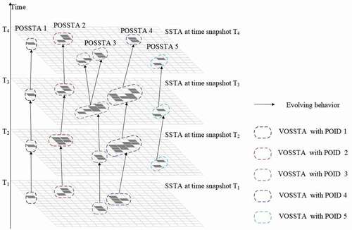
For simplicity, the diagram shown in Figure 1 does not include SOSSTAs. Thus, in the diagram, GDPoSSTA consists of just two datasets – DSPOSSTA and DSVOSSTA. DSPOSSTA includes five POSSTAs – POSSTA1 to POSSTA5. DSVOSSTA includes 16 VOSSTAs. Thirteen development behaviors and two splitting behaviors are also included. At each time snapshot, several independent VOSSTAs exist; e.g. there are four VOSSTAs at time T₁ and five VOSSTAs at time T₂. VOSSTAs with the same POID (Process object identifier) belong to a POSSTA; e.g. POSSTA1, POSSTA2 and POSSTA4 all include four VOSSTAs, POSSTA3 includes five VOSSTAs, and POSSTA5 includes three VOSSTAs.

Compared with other commonly used SSTA products, e.g. Kaplan extended V2 SSTA (Kaplan et al., 1998), the GDPoSSTA dataset has the following advantages.

1. Each VOSSTA has a clear spatial coverage and a thematic attribute at a given time snapshot.

2. The evolution of each SOSSTA between successive VOSSTAs is similar.

3. Each POSSTA shows the changes in an SSTA with time as well as its spatial coverage and thematic characteristics.

4. Each POSSTA evolves from the time of its appearance through its development until it eventually merges, splits or dissipates. That is, from a POSSTA, it is possible to determine when and where SSTAs are generated and dissipate, and also how they develop, merge and split.

2. Methods

A SSTA can be defined as an abnormal increase or decrease in the SST over a specific spatial domain for a specific time (Xue, Song, Qin, Dong, & Wen, 2015a). SSTAs develop in space and time until they dissipate (Liu, Xue, Dong, Wu, & Xu, 2019; Xue et al., 2019a). Here, we define this evolution in terms of a process object named a POSSTA.

2.1. Input data

The original SST product used in this study consisted of monthly global AVHRR data for the period January 1982 to December 2009. These data have a spatial resolution of 4 km. The dataset was obtained from the AVHRR Pathfinder Version 5 and Version 5.1 SST Project (https://data.nodc.noaa.gov/pathfinder/); further details can be found in Kilpatrick, Podestá, and Evans (2001).

2.2. Data processing

The process of producing the POSSTA dataset (DSPOSSTA) from a time-series of satellite-based SST products consisted of four stages, and three intermediate datasets – a SSTA dataset, a VOSSTA dataset and a SOSSTA dataset – were produced during this process. POSSTA also included two relationship files – a SequenceRelationshipFile and an ObjectRelationshipFile – in which the evolution behaviors between VOSSTAs and SOSSTAs were stored. The overall workflow is shown in Figure 2.

Figure 2. Workflow used to produce GDPoSSTA.

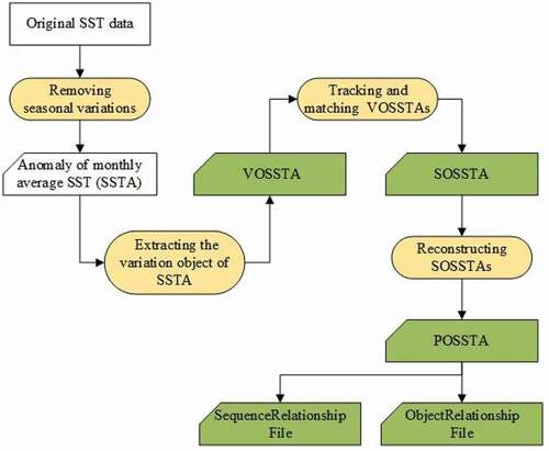
Within a DSPOSSTA, a POSSTA describes the evolution of an SSTA as it develops from its appearance through to eventual dissipation; this process includes one or more SOSSTAs. A SOSSTA consists of several VOSSTAs within successive time snapshots. The evolution of all VOSSTAs belonging to a particular SOSSTA are at similar stages of their evolution – e.g. developing, expanding or weakening. All VOSSTAs belonging to the same SOSSTA are tagged with the same sequence identifier (SID), and all SOSSTAs belonging to the same POSSTA are tagged with the same process object identifier (POID). SequenceRelationshipFile stores details of the type of evolving behavior between SOSSTAs, and ObjectRelationshipFile stores details of the type of evolving behavior between VOSSTAs.

2.3. Key steps

Four key steps are shown in Figure 2

1. Removal of seasonal variations in grid-based SST time-series to generate monthly averaged SSTAs. SSTs vary with the season. These variations are mainly due to changes in solar radiance and need to be removed from climatological sequences before anomalous events can be identified (Xue et al., 2015a). The standard monthly averaged anomaly algorithm, denoted as the z-score (Zhang et al., 2005), is suitable for removing seasonal fluctuations. The z-score takes all the values for a given month from January to December from a long time-series of images and then calculates the mean and standard deviation for that set of monthly values. Each of the original values is then standardized by subtracting the mean and dividing by the standard deviation, as shown in Equation (1)(1) $X_{ij}^{\prime }=\hspace{0.17em}\frac{X_{ij}-{X^{\prime }}_j}{{\delta }_j}\left(j=1,2,...,12\right),$(1) :

(1) $X_{ij}^{\prime }=\hspace{0.17em}\frac{X_{ij}-{X^{\prime }}_j}{{\delta }_j}\left(j=1,2,...,12\right),$(1)

• where i is the year, j is the month from January to December, $\overline{X_j}$ and ${\delta }_j$ are the average value and standard deviation for the j^th month, respectively, and $X_{ij}^{\prime }$ and $X_{ij}$ are the raw and transformed values (of the monthly SST anomaly) obtained from the long-term series of images, respectively. The intermediate dataset produced in this way consists of anomalies in the monthly average SST, i.e. SSTAs.

• (2) Extracting VOSSTAs from spatiotemporal SSTA data. In this step, first the spatiotemporal neighborhoods of SSTAs are reconstructed by taking into account the spatial and temporal continuity of SSTAs as well as their thematic attributes. Second, density-based clustering based on spatial connectivity and temporal evolution is used to define a spatiotemporal neighborhood search window. The spatial proximity, continuity in time and homogeneity in thematic attributes are taken into consideration to obtain the spatiotemporal clustering cores and spatiotemporal density of each grid cell. Finally, the grid cells belonging to the same cluster at each time are taken as being an object, defined as a VOSSTA. More details about the density-based spatiotemporal clustering method can be found in our earlier study (Liu et al., 2018).

• (3) Matching and tracking successive VOSSTAs to form a SOSSTA. In this step, it is assumed that VOSSTAs that are spatially connected, are present at successive times, and have consistent thematic attributes belong to the same SSTA sequence – i.e. a SOSSTA. Thus, the spatial structures, times of appearance and thematic features of VOSSTAs are used as the input features to construct the cost function of VOSSTAs and to then match and track a SOSSTA. These spatial features include the eccentricity, rectangularity, soundness, and shape index of the VOSSTAs; the thematic feature used is the mean SST value of the VOSSTA. For details of the process used to construct the cost function for tracking successive VOSSTAs, please refer to our earlier study (Xue, Liu, Yang, & Wu, 2019b). The Hungarian method is used to solve the assignment problem (Kuhn, 2005).

• (4) Linking and reconstructing SOSSTAs to form a POSSTA

• The SOSSTAs generated using the Hungarian assignment method (Kuhn, 2005), as described in step (3), exhibit no merging or splitting behavior. It is known that SOSSTAs that overlap in space and time are part of the same SSTA evolution process and belong to a POSSTA. Thus, at this step, the spatiotemporal topological relationships between SOSSTAs are used to reshape and construct a POSSTA. During this linking process, one SOSSTA may be linked with two or more SOSSTAs if they consist of the same VOSSTAs. Thus, a recursive loop that links all the related SOSSTAs is designed to reconstruct a new SOSSTA until the new sequence object exhibits no changes. The linking strategy is designed so that if two SOSSTAs from the same time overlap in space, the original SOSSTAs will be replaced by the union of the two SOSSTAs. This is the key to the linking in the recursive loop.

• (5) Identifying different types of evolving behavior from a POSSTA

• Once a POSSTA has been generated, a process-oriented graph model with a pairwise node-edge is used to represent and store the POSSTA; i.e. the VOSSTA is stored as a node, and the evolution between two VOSSTAs is stored as an edge (Xue et al., 2019a). Using an out-degree of the preceding node of an edge, which is given the name PreNOD, and an in-degree of the next node, which is given the name NextNID, the edge relationship can be directly obtained. PreNOD is defined as the number of edges out from the node, and the NextNID is the number of edges coming into the node. The details used to identify the four types of evolving behavior are described below.

  Development: This describes how one object moves from the previous to the current and then to the next snapshot; i.e. there is no interaction with other objects at three successive snapshots. In this case, both PreNOD and NextNID are equal to 1.

  Merging: This describes the merging of two or more objects from the previous snapshot into one object at the current snapshot. In this case, PreNOD is equal to 1 and NextNID is not less than 2.

  Splitting: This describes an interaction in which one object at the current snapshot splits into two or more objects at the next one. In this case, PreNOD is not less than 2 and NextNID is equal to 1.

  Splitting–merging: This describes a situation in which one object splits into two or more objects and simultaneously, one of these objects merges with another one object to form a new object. In this case, both PreNOD and NextNID are not less than 2.

3. Data records

The dataset produced in this study was given the name GDPoSSTA. GDPoSSTA consists of three datasets in one SHP format (ArcGIS format) based on the WGS-84 coordinate system and two relationship files in CSV format (Excel format). The first dataset is DSPOSSTA. This dataset stores details of POSSTAs under file names of the form ProcessObjectDatasets.shp. Each record gives the extent of the spatial coverage, the duration time and the attributes of a process object. The second dataset is DSVOSSTA and stores SOSSTAs in files with names of the form SequenceObjectDatasets.shp. Each of these records contains details of the spatial extent, duration, attributes and type of a sequence object. The last of the three datasets is DSVOSSTA, which contains files with names in the form VariationObjectDatasets.shp. These files store details of VOSSTAs, and each record contains details of the spatial extent, time of occurrence and thematic attributes of these objects. The first type of relationship files have names of the form SequenceRelationship.csv and store details of the evolving behavior between two SOSSTAs, and the other relationship files have names of the form ObjectRelationship.csv and store details of the evolving behavior between two VOSSTAs.

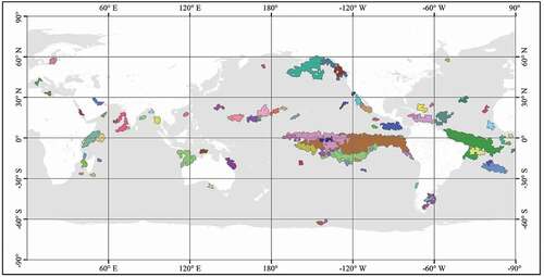
There are a total of 87 records in DSPOSSTA. The spatial distribution of these records is shown in Figure 3, and the fields included in the ProcessObjectDatasets.shp files are shown in Table 2.

Figure 3. Spatial distribution of the 87 POSSTAs in the global ocean for the period January 1982 to December 2009. Different colors represent different POSSTAs.

There are a total of 492 records in DSSOSSTA. The fields in the SequenceObjectDatasets.shp files are shown in Table 3. The SequenceObjectDatasets.shp files are associated with the ProcessObjectDatasets.shp files through a POID field.

Table 2. Fields in ProcessObjectDatasets.shp.

Name	Definition	Comment
FID	LONG	Feature identifier, default field of SHP format
Shape	Polygon	A polygon, default field of SHP format
POID	LONG	POSSTA object identifier
STime	STRING	Time that the POSSTA begins to form
ETime	STRING	Time that the POSSTA dissipates
DurTime	INT	Duration of the POSSTA (units: months)
AvgValue	DOUBLE	Monthly average SSTA value of the POSSTA (units: degree Celsius)
MinValue	DOUBLE	Minimum SSTA value of the POSSTA (units: degree Celsius)
MaxValue	DOUBLE	Maximum SSTA value of the POSSTA (units: degree Celsius)
MinLon	DOUBLE	Minimum longitude of the POSSTA (units: degrees)
MinLat	DOUBLE	Minimum latitude of the POSSTA (units: degrees)
MaxLon	DOUBLE	Maximum longitude of the POSSTA (units: degrees)
MaxLat	DOUBLE	Maximum latitude of the POSSTA (units: degrees)
Abnormal	STRING	An abnormal type of VOSSTA; i.e. a warm or a cold anomaly

Table 3. Fields in SequenceObjectDatasets.shp.

Name	Definition	Comment
FID	LONG	Feature identifier, default field of SHP format
Shape	Polygon	A polygon, default field of SHP format
POID	LONG	As for Table 2; used to associate a POSSTA with SOSSTAs
SQID	STRING	Unique SOSSTA identifier
STime	STRING	Time that the SOSSTA begins to form
ETime	STRING	Time that the SOSSTA ends
DurTime	INT	Duration of the SOSSTA (units: months)
AvgValue	DOUBLE	Monthly average SSTA value of the SOSSTA (units: degree Celsius)
MinValue	DOUBLE	Minimum SSTA value of the SOSSTA (units: degree Celsius)
MaxValue	DOUBLE	Maximum SSTA value of the SOSSTA (units: degree Celsius)
MinLon	DOUBLE	Minimum longitude of the SOSSTA (units: degrees)
MinLat	DOUBLE	Maximum longitude of the SOSSTA (units: degrees)
MaxLon	DOUBLE	Maximum longitude of the SOSSTA (units: degrees)
MaxLat	DOUBLE	Maximum latitude of the SOSSTA (units: degrees)
SeqType	STRING	The type of SOSSTA; i.e. production, development or dissipation sequence (Xue et al., 2019a).
Theta	DOUBLE	The direction of movement of the SOSSTA expressed as an angle measured counterclockwise from a horizontal to the right (range: 0–360°).
Abnormal	STRING	An abnormal type of a VOSSTA; i.e. a warm or a cold anomaly.

There are a total of 1232 records in DSVOSSTA. The fields included in the VariationObjectDatasets.shp files are shown in Table 4. The VariationObjectDatasets.shp files are associated with the SequenceObjectDatasets.shp files by a SQID and with the ProcessObjectDatasets.shp files by a POID.

Table 4. Fields in VariationObjectDatasets.shp.

Name	Definition	Comment
FID	LONG	Feature identifier, default field of SHP format
Shape	Polygon	A polygon, default field of SHP format
POID	LONG	As for Table 2; used to associate a POSSTA with VOSSTAs
SQID	STRING	As for Table 3; used to associate a SOSSTA with VOSSTAs
STID	STRING	Unique VOSSTA identifier
Time	STRING	Time of occurrence of the VOSSTA
Area	DOUBLE	Area covered by the VOSSTA
AvgValue	DOUBLE	SSTA value of the VOSSTA (units: degree Celsius)
MinValue	DOUBLE	Minimum SSTA value within the area covered by the VOSSTA (units: degree Celsius)
MaxValue	DOUBLE	Maximum SSTA value within the area covered by the VOSSTA (units: degree Celsius)
MinLon	DOUBLE	Minimum longitude of the area covered by the VOSSTA (units: degrees)
MinLat	DOUBLE	Minimum latitude of the area covered by the VOSSTA (units: degrees)
MaxLon	DOUBLE	Maximum longitude of the area covered by the VOSSTA (units: degrees)
MaxLat	DOUBLE	Maximum latitude of the area covered by the VOSSTA (units: degrees)
CoreLon	DOUBLE	Central longitude of the area covered by the VOSSTA (units: degrees)
CoreLat	DOUBLE	Central latitude of the area covered by the VOSSTA (units: degrees)
Abnormal	STRING	An abnormal type of a VOSSTA; i.e. a warm or a cold anomaly

A total of 326 evolving behaviors of SOSSTAs are stored in the SequenceRelationship.csv files. The fields that comprise these files are shown in Table 5. A total of 1066 evolving behaviors of VOSSTAs are stored in the ObjectRelationship.csv files. The fields that comprise these files are shown in Table 6.

Table 5. Fields in SequenceRelationship.csv.

Name	Definition	Comment
SQID_1	STRING	SOSSTA 1 object identifier
SQID_2	STRING	SOSSTA 2 object identifier
Relationship	STRING	Type of evolving behavior between the two SOSSTAs; i.e. development, splitting, merging or splitting–merging
Abnormal	STRING	An abnormal type of a VOSSTA; i.e. a warm or a cold anomaly

Table 6. Fields in ObjectRelationship.csv.

Name	Definition	Comment
PRIOR_STID	STRING	SOSSTA object identifier at previous time snapshot
NEXT_STID	STRING	SOSSTA object identifier at next time snapshot
Relationship	STRING	Type of evolving behavior between the two VOSSTAs; i.e. development, splitting, merging or splitting–merging
Abnormal	STRING	An abnormal type of a VOSSTA; i.e. a warm or a cold anomaly

All of the above datasets are available from the ScienceDB record associated with this publication. Further details of the available files are listed in Table 7.

Table 7. Details of the files contained in the ScienceDB record.

No	File List	Description
1	ProcessObjectDatasets.dbf	ArgGIS SHP files in the ProcessObjectDatasets
2	ProcessObjectDatasets.prj
3	ProcessObjectDatasets.sbn
4	ProcessObjectDatasets.sbx
5	ProcessObjectDatasets.shp
6	ProcessObjectDatasets.shp.xml
7	ProcessObjectDatasets.shx
8	SequenceObjectDatasets.dbf	ArgGIS SHP file in the SequenceObjectDatasets
9	SequenceObjectDatasets.prj
10	SequenceObjectDatasets.sbn
11	SequenceObjectDatasets.sbx
12	SequenceObjectDatasets.shp
13	SequenceObjectDatasets.shp.xml
14	SequenceObjectDatasets.shx
15	VariationObjectDatasets.dbf	ArgGIS SHP files in the VariationObjectDatasets
16	VariationObjectDatasets.prj
17	VariationObjectDatasets.sbn
18	VariationObjectDatasets.sbx
19	VariationObjectDatasets.shp
20	VariationObjectDatasets.shp.xml
21	VariationObjectDatasets.shx
22	ObjectRelationship.csv	Relationship files in which the evolving behaviors between VOSSSTAs are stored
23	SequenceRelationship.csv	Relationships files in which the evolving behaviors between SOSSTAs are stored

4. Technical validation

Each GDPoSSTA consists of three kinds of objects: a POSSTA, a SOSSTA and a VOSSTA. A SOSSTA is an intermediate object that consists of series of VOSSTAs; thus, we can evaluate a VOSSTA and a POSSTA to test a GDPoSSTA.

4.1. Validation of VOSSTAs

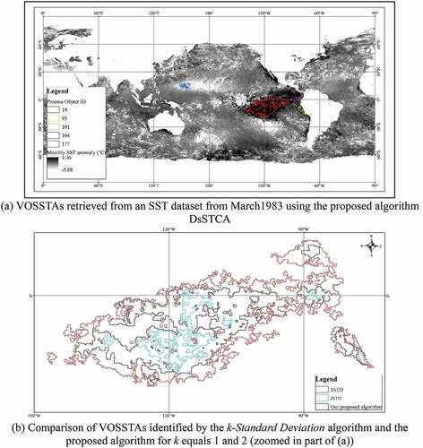
The core idea behind the extraction of VOSSTAs from long-term grid-based SST products is the use of a density-based spatiotemporal clustering algorithm; i.e. DcSTCA. This algorithm was developed in our earlier study (Liu et al., 2018). In DcSTCA, the grid cells that belong to the same cluster at a given time are taken as forming one VOSSTA. As a VOSSTA relates to an abnormal increase or decrease in SST over a specific spatial domain, we used k-Standard Deviation, which is a spatiotemporal statistical algorithm, to identify objects and evaluate the VOSSTA datasets. The identified objects were given the name VOSSTA-Ks. The k-Standard Deviation algorithm first identifies the abnormal grid cells in a time-series: abnormal means that their values are greater than k times the standard deviation of the long-term SST values. The abnormal grid cells from a given time are then spatially connected to form an object; i.e. a VOSSTA-K. Figure 4(a) shows five VOSSTAs that were retrieved from a remote-sensing SST dataset from March 1983 using the proposed DcSTCA. The background consists of the monthly SSTA data. Figure 4(b) shows a comparison between the results obtained using the k-Standard Deviation algorithm and our proposed algorithm. The results show that our VOSSTAs are between VOSSTA-1s and VOSSTA-2s.

Figure 4. Comparison of the spatial distribution of VOSSTAs identified using the proposed DcSTCA and k-Standard Deviation. (a) VOSSTAs retrieved from an SST dataset from March 1983 using the proposed algorithm DsSTCA. (b) Comparison of VOSSTAs identified by the k-Standard Deviation algorithm and the proposed algorithm for k equals 1 and 2 (zoomed in part of (a)).

4.2. Validation of POSSTAs

The tracking of a POSSTA and its construction from successive VOSSTAs depends on the PoAIR algorithm that was introduced in our earlier study (Xue et al., 2019b). PoAIR has been evaluated using 10 simulated process-oriented datasets and the results compared to those obtained using the original Thunderstorm Identification, Tracking, Analysis and Nowcasting algorithm (TITAN) algorithm (Dixon & Wiener, 1993). Table 8 shows a comparison of the tracking of process objects in terms of the probability of detection (POD). This table is modified from the results shown as Figure 9 and Table 3 in Xue et al. (2019b). Table 9 shows a comparison of the results for the identified evolving behaviors between process objects, also given in terms of the POD. The results shown in these two tables demonstrate that PoAIR performs better than TITAN in terms of POD for both basic and complicated process objects, and that PoAIR clearly outperforms TITAN when dealing with the splitting, merging, and merging–splitting behaviors of VOSSTAs.

Table 8. Comparison of the tracking of process objects by the proposed PoAIR algorithm and TITAN (Modified from Figure 9 and Table 3 in Xue et al. (2019b)).

	Process object 1				Process object 2				Process object 3				Process object 4
	PoAIR		TITAN		PoAIR		TITAN		PoAIR		TITAN		PoAIR		TITAN
NTO	10				22				19				17
NDO	6	4	6	4	20		12+1	9	18		15+1		17		10+2	7
POD (%)	60.00		60.00		90.91		54.54		94.70		78.95		100.00		58.82
	Process object 5				Process object 6				Process object 7
	PoAIR		TITAN		PoAIR		TITAN		PoAIR		TITAN
NTO	11				22				19
NDO	11		18+1	3	20	2       9	9        9	2	19	11	6	2
POD (%)	100.00		72.72		90.91		45		100		57.89
	Process object 8				Process object 9				Process object 10
	PoAIR		TITAN		PoAIR		TITAN		PoAIR		TITAN
NTO	25				8				18
NDO	25		12       8	2       2	5	3	5	3	18		12+1	6+1
POD (%)	100.00		48.00		62.50		62.50		100.00		66.67

Table 9. Comparison of identified evolving behaviors by the proposed PoAIR algorithm and TITAN.

	Developing		Merging		Splitting		Splitting–merging
	PoAIR	TITAN	PoAIR	TITAN	PoAIR	TITAN	PoAIR	TITAN
NTE	109		18		22		14
NDE	100	81	16	8	16	12	12	6
POD (%)	91.74	74.31	88.89	44.44	72.73	54.56	85.71	42.86

In Table 8, NTO (number of target objects) means the number of real abnormal variation objects belonging to the same process object and NDO (number of detected objects) means the number of abnormal variation objects detected by TITAN or the PoAIR algorithm. If a process object is tracked as two or more independent process objects, NDO will have two or more values; e.g. process object 1 was tracked as two process objects by both TITAN and the PoAIR algorithm. In this case, one process object includes six variation objects and the other process object includes four variation objects. In such a situation, the POD for the larger NDO is taken as the probability of detection; thus, the POD for both TITAN and the PoAIR algorithm is 60.00%. If a noise object is identified as an object belonging to a process object, the NDO is taken as the number of detected objects plus the number of noise objects; e.g. for process object 2, the NDO for TITAN is 12 + 1. Here, 12 is the number of detected objects and 1 is the number of noise objects; both types of object are regarded as belonging to the same process object 2 by TITAN.

The NTE (number of targeted evolving behaviors) means the number of real evolving behaviors linking all the process objects. NDE (number of detected evolving behaviors) means the number of evolving behaviors detected by TITAN or by the PoAIR algorithm.

4.3. Analysis of a specific POSSTA

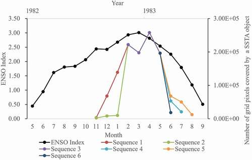
A POSSTA describes the evolution of an SSTA from its origin through its development until it dissipates in space and time. The evolution of SSTAs is closely related to global climate change (McPhaden et al., 2006; Song et al., 2016; Xue et al., 2019a); e.g. ENSO and the Indian Ocean Dipole (IOD). Thus, we analyzed the dynamic evolution of a specific POSSTA and its relationship with the ENSO to indirectly test the applicability of the use of POSSTAs. Figure 5 depicts the evolution of the selected POSSTA in the Eastern Pacific Ocean from November 1982 to August 1983. Using the area covered by the VOSSTA at a particular time to represent the intensity of the POSSTA, Figure 6 shows that there is a close relationship between the evolution of the POSSTA and the ENSO event that lasted from May 1982 to September 1983. From Figures 5 and 6, when and where the SSTA originated and dissipated as well as when and where the SSTA became stronger (merging) and weaker (splitting) can be determined. Analyzing the evolution of SSTAs will give a better understanding of the evolution of the ENSO, and POSSTAs provide more information than that provided by static SSTAs.

Figure 5. The POSSTA that was selected for analysis. The black polygons denote VOSSTAs; the arrows denote the evolution of the VOSSTAs. A total of six evolutionary sequences are shown by the six colored lines. The background is the monthly SSTA.

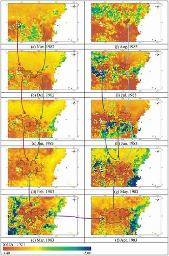
Figure 6. Graph showing the close relationship between the selected POSSTA and an ENSO event.

5. User notes

In contrast to SSTA remote-sensing datasets, the GDPoSSTA dataset provides information about not only the spatial distribution of changes in SSTAs – i.e. SSTA snapshots – but also information about the evolution of SSTAs with time. The evolution of SSTAs in space and time plays a much more important role in global or regional climate change than their static characteristics in space. For example, the dissipation or origin of a POSSTA, a spatial distribution of evolution relationship, and its migration in space are all closely related to different types of ENSO: i.e. the Eastern Pacific ENSO, Central Pacific ENSO and MIX ENSO.

The files in the three datasets that make up the GDPoSSTA are in SHP format. This is a commonly used format in GIS, which means that the files can easily be read by commercial GIS software such as ArcGIS and MapGIS, as well as open-source GIS software such as QGIS and GRASS. The two types of relationship file, which are in CSV format, can be read by Microsoft Excel.

The GDPoSSTA source code will be provided upon request for the purpose of replicating the reanalysis data described in this paper. The code may be requested from the corresponding author by email.

Acknowledgments

The research presented in this paper was funded by the Strategic Priority Research Program of the Chinese Academy of Sciences – Grant No. XDA19060103 – and the National Natural Science Foundation of China – Grant Nos. 41671401 and 41976184. The authors are grateful to the US National Oceanographic Data Center and the GHRSST (http://pathfinder.nodc.noaa.gov) for providing the AVHRR Pathfinder Version 5.0 and Version 5.1 data.

Disclosure statement

No potential conflict of interest was reported by the author(s).

Data Availability Statement

The data that support the findings of this study are openly available in ScienceDB at http://www.doi.org/10.11922/sciencedb.j00076.00090.

Additional information

Funding

This work was supported by the Strategic Priority Research Program of the Chinese Academy of Sciences [XDA19060103]; National Natural Science Foundation of China [41671401, 41976184].

Notes on contributors

Cunjin Xue

Cunjin Xue, received a B.S. degree in Geographical Science from Shandong Normal University in 2002, an M.E. degree in Cartography and Geographical Information Systems from Wuhan University in 2005 and his PhD degree in Cartography and Geographical Information System from the Institute of Geographic Sciences and Natural Resources Research, Chinese Academy of Sciences in 2008. He is a professor at the Aerospace Information Research Institute, Chinese Academy of Sciences. His main research interests are marine spatiotemporal data mining and its applications. He has published more than 80 papers and holds four patents.

References

- Banzon, V. F., Reynolds, R. W., Stokes, D., & Xue, Y. (2014). A 1/4°-Spatial-resolution daily sea surface temperature climatology based on a blended satellite and in Situ analysis. Journal of Climate, 27(21), 8221–8228.
- Cao, M., Mao, K., Yan, Y., Shi, J., Wang, H., Xu, T., … Yuan, Z. (2021). A new global gridded sea surface temperature data product based on multisource data. Earth System Science Data, 13(5), 2111–2134.
- Dai, A. (2016). Future warming patterns linked to today’s climate variability. Scientific Reports, 6(1), 19110.
- Ding, R., Tseng, Y., Li, J., Sun, C., Xie, F., & Hou, Z. (2019). Relative contributions of North and South Pacific sea surface temperature anomalies to ENSO. Journal of Geophysical Research: Atmospheres, 124, 6222–6237.
- Dixon, M., & Wiener, G. (1993). TITAN: Thunderstorm Identification, Tracking, Analysis, and Nowcasting—A radar-based methodology. Journal of Atmospheric and Oceanic Technology, 10(6), 785–797.
- GCOS. (2011). Systematic observation requirements for satellite-based products for climate, 2011 update. GCOS Report 154. WMO.
- Guo, Y., Zhang, R., Wen, Z., Li, J., Zhang, C., & Zhou, Z. (2021). Understanding the role of SST anomaly in extreme rainfall of 2020 Meiyu season from an interdecadal perspective. Science China Earth Sciences, 64(10), 1–14.
- Hollmann, R., Merchant, C. R., Saunders, R., Downy, C., Buchwitz, M., Cazenave, A., … Wagner, W. (2013). The ESA climate change initiative: Satellite data records for essential climate variables. Bulletin of the American Meteorological Society, 94(10), 1541–1552.
- Kaplan, A., Cane, M., Kushnir, Y., Clement, A., Blumenthal, M., & Rajagopalan, B. (1998). Analyses of global sea surface temperature 1856-1991. Journal of Geophysical Research, 103(C9), 18567–18589.
- Kawale, J., Stefan, L., Arjun, K., Michael, S., Peter, S., Vipin, K., … Semazzi, F. (2013). A graph-based approach to find teleconnections in climate data. Statistical Analysis and Data Mining: The ASA Data Science Journal, 6(3), 158–179.
- Kilpatrick, K. A., Podestá, G. P., & Evans, R. (2001). Overview of the NOAA/NASA advanced very high resolution radiometer pathfinder algorithm for sea surface temperature and associated matchup database. Journal of Geophysical Research: Oceans, 106(C5), 9179–9197.
- Kuhn, H. W. (2005). The Hungarian method for the assignment problem. Naval Research Logistics, 52(1), 7–21.
- Legeckis, R., & Zhu, T. (1997). Sea surface temperatures from the GOES-8 Geostationary Satellite. Bulletin of the American Meteorological Society, 78(9), 1971–1983.
- Liao, Z. H., Dong, Q., Xue, C. J., Bi, J. W., & Wan, G. T. (2017). Reconstruction of daily sea surface temperature based on radial basis function networks. Remote Sensing, 9(11), 1204.
- Liu, J. Y., Xue, C. J., Dong, Q., Wu, C. B., & Xu, Y. F. (2019). A process-oriented spatiotemporal clustering method for complex trajectories of dynamic geographic phenomena. IEEE Access, 7, 155951.
- Liu, J. Y., Xue, C. J., He, Y. W., Dong, Q., Kong, F. P., & Hong, Y. L. (2018). Dual-constraint spatiotemporal clustering approach for exploring marine anomaly patterns using remote sensing products. Journal of Selected Topics in Applied Earth Observations and Remote SensSensing, 11(11), 3693–3796.
- McClain, E. P., Pichel, W. G., & Walton, C. C. (1985). Comparative performance of AVHRR-based multichannel sea surface temperatures. Journal of Geophysical Research, 90(C6), 11587–11601.
- McPhaden, M. J., Zebiak, S. E., & Glantz, M. H. (2006). ENSO as an integrating concept in earth science, 314(5806), 1740–1745.
- Merchant, C. J., Borgne, P., Borgne, L. E., Marsouin, A. M., & Roquet, H. R. (2008). Optimal estimation of sea surface temperature from split-window observations. Remote Sensing of Environment, 112(5), 2469–2484.
- Murtugudde, R., Wang, L. P., Hackert, E., Beauchamp, J., Christian, J., & Busalacchi, A. J. (2004). Remote sensing of the Indo-Pacific region: Ocean colour, sea level, winds and sea surface temperatures. International Journal of Remote Sensing, 25(7–8), 1423–1435.
- Ping, B., Su, F. Z., & Meng, Y. S. (2015). Reconstruction of satellite-derived sea surface temperature data based on an improved DINEOF algorithm. IEEE Journal of Selected Topics in Applied Earth Observations and Remote Sensing, 8(8), 4181–4188.
- Reynolds, R. W., Rayner, N. A., Smith, T. M., Stokes, D. C., & Wang, W. Q. (2002). An improved in situ and satellite SST analysis for climate. Journal of Climate, 15(13), 1609–1625.
- Reynolds, R. W., Smith, T. M., Liu, C., Chelton, D. B., Casey, K. S., & Schlax, M. G. (2007). Daily high-resolution-blended analyses for sea surface temperature. Journal of Climate, 20(22), 5473–5496.
- Saha, K.…, Zhao, K., Xuepeng, X., Zhang, H.-M., Casey, K. S., Zhang, D., Sheekela, B-Y.,Kilpatrick, K.D., Evans, R.H., Ryan, T., Relph, J.M. (2018). AVHRR Pathfinder version 5.3 level 3 collated (L3C) global 4km sea surface temperature for 1981-Present. NOAA National Centers for Environmental Information. Dataset. doi: https://doi.org/10.7289/v52j68xx.
- Saulquin, B., Fablet, R., Mercier, G., Demarcq, H., Mangin, A., & Andon, O. H. F. (2014). Multiscale event-based mining in geophysical time series: Characterization and distribution of significant time-scales in the sea surface temperature anomalies relatively to ENSO periods from 1985 to 2009. IEEE Journal of Selected Topics in Applied Earth Observations and Remote Sensing, 7(8), 3543–3552.
- Song, W. J., Dong, Q., & Xue, C. J. (2016). A classified El Niño index using AVHRR remote-sensing SST data. International Journal of Remote Sensing, 37(2), 403–417.
- Steinbach, M., Tan, P., Boriah, S., Kumar, V., Klooster, S., & Potter, C. (2006, May 23–24). The application of clustering to earth science data: Progress and challenges. In Proceedings of the 2nd NASA data mining workshop: issues and applications in earth science data (pp. 1–6). Pasadena, CA.
- Walton, C. C., Pichel, W. G., Sapper, J. F., & May, D. A. (1998). The development and operational application of nonlinear algorithms for the measurement of sea surface temperatures with the NOAA polar-orbiting environmental satellites. Journal of Geophysical Research, 103(C12), 27999–28012.
- Wentz, F. J. T., Meer, C. T., Gentemann, M. C., & Brewer, M. (2014). Remote sensing systems AQUA AMSR-E daily, weekly, and monthly. Environmental suite on 0.25 deg grid, Version 8.2. Remote Sensing Systems. Santa Rosa, CA. Retrieved from www.remss.com/missions/amsr
- Wu, T. S., Song, G. J., Ma, X. J., Xie, K. Q., Gao, X. P., & Jin, X. X. (2008). Mining geographic episode association patterns of abnormal events in global earth science data. Science in China Series E: Technological Sciences, 51(S1), 155–164.
- Xu, Y. F., Xue, C. J., & He, Y. W. (2021, August 20). A dataset of sea surface temperature abnormal change process objects (GDPoSSTA V1.0), Global ocean 1982-2009. V1. Science Data Bank. Retrieved from https://datapid.cn/31253.11.sciencedb.j00076.00090.
- Xue, C. J., Dong, Q., & Qin, L. (2015b). A cluster-based method for marine sensitive object extraction and representation. Journal of Ocean University of China, 14(4), 612–620.
- Xue, C. J., Liu, J. Y., Yang, G., & Wu, C. (2019b). A process-oriented method for tracking rainstorms with a time-series of raster datasets. Applied Sciences, 9(12), 2468.
- Xue, C. J., Song, W. J., Qin, L. J., Dong, Q., & Wen, X. Y. (2015a). A spatiotemporal mining framework for abnormal association patterns in marine environments with a time series of remote sensing images. International Journal of Applied Earth Observation and Geoinformation, 38, 105–114.
- Xue, C. J., Wu, C. B., Liu, J. Y., & Su, F. Z. (2019a). A novel process-oriented graph storage for dynamic geographic phenomena. ISPRS International Journal of Geo-Information, 8(2), 100.
- Yang, J., Gong, P., Fu, R., Zhang, M., Chen, J., Liang, S., … Dickinson, R. (2013). The role of satellite remote sensing in climate change studies. Nature Climate Change, 3(10), 875–883.
- Yu, S. Y., Fan, L., Zhang, Y., Zheng, X. T., & Li, Z. (2021). Reexamining the Indian summer monsoon rainfall–ENSO relationship from its recovery in the 21st century: Role of the Indian ocean SST anomaly associated with types of ENSO evolution. Geophysical Research Letters, 48(12), e2021GL092873.
- Zhang, P. S., Tan, P. N., Steinbach, M., Kumar, V., Shekhar, S., Klooster, S., & Potter, C. (2005). Discovery of patterns in the earth science data using data mining. In J. Zurada & M. Kantardzic (Eds.), Next generation of data mining applications. Wiley-IEEE Press, 167-188, February 2005, ISBN: 0-471-65605-4. (eBook).