Pan-Arctic ocean wind and wave data by spaceborne SAR

ABSTRACT

The Arctic is one of the most significant changing areas on the Earth under the climate change scenario. More regions in the Arctic are becoming ice-free oceans in the melting season or through the whole year. Therefore, ocean wind and wave, as the two most important parameters in the air–sea interface, are drawing significant attention to the Arctic Ocean. Scatterometer and radar altimeter are the two traditional remote sensing instruments for ocean wind and wave observations, while the former is limited by coarse spatial resolution and the latter has small spatial coverage. Wind and wave data in high spatial resolution and wide coverage by synthetic aperture radar (SAR) are currently lacking in the Arctic Ocean. We developed an ocean wind and wave dataset by Sentinel-1 SAR in the pan-Arctic Ocean (above 60°N), covering January 2017 to May 2021. By comparing with sea surface wind speed data of scatterometer, the SAR-retrieved wind data achieve an accuracy of 1.23 m/s, in terms of root mean square error (RMSE). Compared with significant wave height data of radar altimeter, the SAR retrievals have an RMSE of 0.66 m. The data records are in the standard NetCDF-4 format. The dataset is publicly available at: http://www.dx.doi.org/10.11922/sciencedb.00834.

KEYWORDS:

• Arctic
• synthetic aperture radar (SAR)
• ocean wind
• ocean wave

1. Introduction

Ocean wind and wave measurements and observations have great significance for studying the interaction between sea ice and ocean dynamic process in the Arctic Ocean (Asplin, Galley, Barber, & Prinsenberg, 2012; Kodaira et al., 2021; Stopa et al., 2018). Along with the decline of sea ice extent in the Arctic, the Northern Sea Route (NSR) has been drawing attention. Therefore, shipping safety in the complicated marginal ice zone (MIZ) is a crucial consideration for the utilization of the route. Ocean wind and wave naturally play an important role in navigation safety (Inoue et al., 2015; Podgórski & Rychlik, 2014). Moreover, strong winds and high waves also tend to increase in the Arctic Ocean (Waseda et al., 2018). Compared with other basins, in situ wind and wave measurements in the Arctic Ocean are even coarser partially due to inclement weather conditions and sea ice states. Therefore, accurate observations of ocean wind and wave by satellite remote sensing are crucial.

Spaceborne scatterometers and radar altimeters (RA) have been two reliable instruments for global ocean wind and wave observations for a few decades (e.g. Ribal & Young, 2019; Young, Zieger, & Babanin., 2011). Generally, spaceborne scatterometers have large swath width of a few hundreds of kilometers and can provide wind data with a relatively coarse spatial resolution of 25 km or 12.5 km. To some extent, such coarse resolution can lose fine structures of sea surface wind field. Different from scatterometer as a side-looking radar, RA obtains the sea surface reflected radar signal at nadir. Therefore, ocean wave or wind measurements are limited to the footprint of RA, which generally varies from 6 km to 15 km. Applications of ocean wind and wave data by scatterometers and RAs in the Arctic Ocean also have been reported (e.g. Ali, Bhat, Long, Bharadwaj, & Bourassa, 2013; Li, Shen, Hou, He, & Bi, 2018; Ozbahceci, 2020). Besides the spaceborne radar sensors, the coastal-based High-Frequency (HF) Radar (Huang, Gill, Wen, Wen, & Hou, 2002; Rubio et al., 2017) and the shipborne X-band marine radar (Huang, Liu, & Gill, 2017) can be alternatives to measure wind and wave information.

Both ocean wind and wave measured by spaceborne synthetic aperture radar (SAR) is not a new topic. With respect to the sea surface wind (SSW) retrieval by SAR, the most common approach is to apply the geophysical model function (GMF) (e.g. Stoffelen & Anderson, 1997), which empirically relates radar backscatter with sea surface wind and imaging geometry (incidence angle and azimuth direction). Often, we have to use external wind direction from weather prediction/forecast model to resolve the sea surface wind speed (SSWS) by SAR data (e.g. Thompson & Beal, 2000) based on the GMF functions. Compared with SSW by scatterometer, the SAR retrievals can have a high spatial resolution up to approximately 300 m (Li & Lehner, 2013).

Retrieval of ocean wave information, including two-dimensional wave spectrum or integral wave parameters by spaceborne SAR data, has been investigated for a few decades. The difficulty is that imaging of ocean waves by SAR is generally considered nonlinear (Alpers, Ross, & Rufenach, 1981), which leads to a complicated inversion process (Hasselmann, Brüning, Hasselmann, & Heimbach, 1996), needing the so-called first guess spectrum generally provided by ocean wave modeling. To overcome the dependence of traditional retrievals on first guess spectrum, empirical algorithms were proposed for various spaceborne SAR data (Li, Lehner, & Bruns, 2011; Schulz-Stellenfleth, König, & Lehner, 2007; Stopa & Mouche, 2017). They directly yield integral ocean wave parameters without needing external information. Although it is difficult to retrieve ocean wave information by spaceborne SAR data, efforts have been made to promote SAR ocean wave data, e.g. the swell spectrum data by the ENVISAT/ASAR (Ardhuin, Chapron, & Collard, 2009; Li, 2016) and Sentinel-1 (S1) SAR (Khan, Echevarria, & Hemer, 2021) wave mode data. Recently, Li and Huang (2020) processed the ASAR wave mode data in its entire life time (2002–2012) to full sea state parameters of significant wave height (SWH) and mean wave period (MWP) based on the empirical algorithm.

Besides the complicated procedures of retrieving ocean waves by spaceborne SAR data, relatively coarse temporal and spatial coverages of SAR acquisitions over the global ocean limit its wide application. So far, only the specific wave mode data with a relatively small size of a few kilometers are acquired continuously over global oceans. The launch of Sentinel-1A (April 2014) and 1B (April 2016) forms a constellation, which significantly increases temporal and spatial coverages, particularly in high latitude regions. As polar regions are being paid special attention in the scenario of climate change, European Space Agency (ESA) guarantees the twins to extensively acquire SAR data in extra-wide swath (~400 km) and Interferometric wide swath (~250 km) modes. Moreover, these data are acquired in dual-polarization of Horizontal-Horizontal (HH) and Horizontal-Vertical (HV) or Vertical-Vertical (VV) and Vertical-Horizontal (VH), which are particularly powerful for sea ice monitoring in the polar regions (e.g. Leigh, Wang, & Clausi, 2014; Li, Sun, & Zhang, 2021). We previously found that the S1 twins can acquire data covering most of the Arctic Ocean by 2–3 days.

Inspired by the extensive acquisitions of the S1 data over the Arctic, we have been working on algorithms development of deriving ocean wind (Li, Qin, & Wu, 2020) and wave (Wu, Li, & Huang, 2021) information by S1 data. Based on the developed algorithms, we have processed the S1 data acquired in the pan-Arctic Ocean (above 60°N) through January 2017 to May 2021 to SSW and SWH data in the standard format of NetCDF-4. Such data in high spatial resolution (~2 km) in the Arctic Ocean are highly demand for scientific research and shipping navigation. In this paper, we present the development of the S1-derived ocean wind and wave products, including the processing method (Section 3), designing of data records and quality control flags (Section 4), and comprehensive validation experiments (Section 5).

2. Materials

2.1. Sentinel-1 spaceborne SAR data

The S1 EW mode data are used in this study, which have a swath width of 400 km and a pixel size of 40 m × 40 m. The two satellites of S1A and S1B have been acquired the EW mode data in the Arctic with short temporal intervals and large spatial coverage. These data are generally acquired with a polarization combination of HH and HV. While the HV-polarized data are dedicated for sea ice monitoring (e.g. Li et al., 2021; Wang & Li, 2021), the HH-polarized data (one example shown in Figure 1) are used for retrieval of sea surface wind and ocean wave height.

Figure 1. The S1 EW sub-images in HH polarization acquired by S1A at 7:47 UTC on 1 December 2018 in the Norwegian sea presenting a mixture of sea ice (upper-left corner) and open water, in which wind streaks are visible. The wave-like patterns are visible in the zoomed sub-image (right panel). the image ID is S1A_EW_GRDM_1SDH_20181201T074714_20181201T074814_024829_02BBC2_BE2B.SAFE.

The used S1 data are Level-1 Ground Range Detected (GRD) products in which the Digital Number (DN) values are stored. By radiometric calibration of DN data, the Normalized Radar Cross Section (NRCS, denoted ${\sigma }_0$) is obtained (ESA, 2016):

(1) $\begin{array}{c}{\sigma }_0=\frac{D{N}^2-n}{k_s^2}\end{array}$(1)

where n is the noise vector and $k_s$ is the calibration factor, which are given in the S1 metadata product.

Based on the previously developed methods of retrieving SWH and SSWS by S1 EW data in HH polarization, which are described in Section 3, we have processed 54,172 S1 EW scenes acquired from January 2017 to May 2021 to wind and wave products in the Arctic. The amount of processed EW data in each month during this period is shown in Figure 2. Influenced by the sea ice melting and freezing, the number of available products changes seasonally. The minimum and maximum data amount are achieved in March and September, respectively, when the sea ice has the largest and smallest coverage of the year in the Arctic. Among the fully processed EW data, 25,633 scenes from June 2018 to June 2020 were used to validate SSWS and SWH retrievals by comparing with scatterometer and RA wind and wave data.

Figure 2. Amount of S1 EW images processed in the pan-Arctic ocean for producing wind and wave products in each month through January 2017 to May 2021.

2.2. ASCAT and RA wind and wave data

This study collected the scatterometer ASCAT SSW data from the European Organization for the Exploitation of Meteorological Satellites (EUMETSAT, https://archive.eumetsat.int/usc/) to validate the S1-retrieved SSWS results. The ASCAT wind products under all weather conditions are used, which have a spatial resolution of 25 km × 25 km.

Four Radar Altimeters (RA) were used in this study, i.e. CryoSat-2, Jason-2, Jason-3, and SARAL, to validate the S1-retrieved SSWS and SWH. The CryoSat-2 data are accessed from the European Space Agency (ESA, http://science-pds.cryosat.esa.int/), and other RAs data are from EUMETSAT. These RA data are screened with the value for “flag_instr_op_mode” of 1 (for CryoSat-2 data) or “qual_swh” of 0 (for Jason-2, Jason-3 and SARAL data).

Before using the RA data from multiple missions for validation, cross-comparisons among them were conducted. Table 1 shows the cross-comparisons of SWH data among the four RA missions. Both bias and RMSE suggest that they have good agreements with each other, except that the comparison between CryoSat-2 and SARAL has a bias of −0.11 m, slightly higher than other comparisons. With respect to cross-comparisons of SSWS data (Table 2), it is found that the RMSEs are very close to each other. However, the bias shows some fluctuations. Notably, the comparison between CryoSat-2 and SARAL has a relatively high bias of −0.39 m/s. Considering that the RMSEs achieved in the cross-comparisons for SWH and SSWS are insignificant, we treated the data from the four RA missions as a whole Table 3.

Table 1. Cross-comparison of SWH data between June 2018 and June 2020 from the four RA missions over the pan-Arctic ocean.

	Jason-2		Jason-3		SARAL
	Bias (m)	RMSE (m)	Bias (m)	RMSE (m)	Bias (m)	RMSE (m)
CryoSat-2	−0.02	0.02	−0.03	0.02	−0.11	0.02
Jason-2	/	/	0.03	0.01	−0.01	0.03
Jason-3	/	/	/	/	−0.01	0.03

Table 2. Cross-comparison of SSWS data between June 2018 and June 2020 from the four RA missions over the pan-Arctic ocean.

	Jason-2		Jason-3		SARAL
	Bias (m/s)	RMSE (m/s)	Bias (m/s)	RMSE (m/s)	Bias (m/s)	RMSE (m/s)
CryoSat-2	−0.20	0.02	−0.11	0.03	−0.39	0.02
Jason-2	/	/	0.15	0.00	−0.13	0.03
Jason-3	/	/	/	/	−0.20	0.03

Table 3. Summary of the previous comparisons of S1 retrievals of SSWS and SWH with different reference data (Li, Qin, & Wu, 2020) and (Wu, Li, & Huang, 2021).

Retrievals	Reference data	No. Col.	Bias	RMSE	Scatter Index (SI)
SSWS	ASCAT	1,740,509	0.20 m/s	1.27 m/s	15.17%
	In situ Buoy	305	0.09 m/s	1.41 m/s	22.68%
	XueLong R/V	23	−0.23 m/s	1.16 m/s	14.59%
SWH	RA	31,532	0.02 m	0.63 m	21.07%
	CFOSAT/SWIM (nadir)	32,403	0.15 m	0.60 m	18.98%

2.3. ERA5 reanalysis model data

ERA5 is the fifth generation ECMWF (European Centre for Medium-Range Weather Forecasts) reanalysis dataset for the global climate and weather (Hersbach et al., 2020). The global wind vector data of the ERA5 reanalysis model are hourly available with a grid size of 0.25° × 0.25°. In this study, its wind direction data are used as the input parameter to the SSWS retrieval. The ERA5 data are downloaded through the Copernicus Climate Change Service (https://cds.climate.copernicus.eu/).

2.4. Sea ice concentration data

The Advanced Microwave Scanning Radiometer 2 (AMSR2) sea ice concentration data, with a spatial resolution of 6.25 km, are used to exclude the SAR images with sea ice proportion over 85% from processing to ocean wind and wave data. The AMSR2 data are provided by the University of Bremen (https://seaice.uni-bremen.de/data/).

2.5. IMS sea ice cover data

The interactive multi-sensor snow and ice mapping system (IMS) is an operational software package for analyzing snow and ice coverage (Helfrich, Li, Kongoli, Nagdimunov, & Rodriguez., 2019), which can provide daily sea ice coverage data in the Northern Hemisphere with a grid size of 1 km × 1 km. This study used this data to mask sea ice cover and land in S1 EW images. The IMS data are released by the U.S. National Ice Center (USNIC, https://usicecenter.gov/Products/).

3. Methods

Figure 3 shows the flowchart of the proposed methodology to derive ocean wind and wave products by S1 SAR data in the Arctic Ocean, which is composed of three components, i.e. pre-processing of the SAR data, producing of the SSW and SWH data. The entire processing chain is automatic. In the following subsections, it is described in detail.

Figure 3. Flowchart of producing S1-based SSW and SWH data in the pan Arctic ocean.

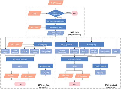
3.1. Pre-processing of the S1 EW data

As SAR images may contain sea surface features (e.g. surface films, rain cells) or targets (e.g. ships, platforms), we have to use an automatic approach to select SAR images presenting homogeneous sea surface for retrieval of sea surface wind and wave. A homogeneity factor was proposed by Schulz-Stellenfleth and Lehner (2004):

(2) ${\xi }_H={\left(\sum _k\overline{mean}\left({\hat{\mathrm{\Phi }}}_k\right)\right)}^{-1}\sum _k\frac{\overline{var}\left({\hat{\mathrm{\Phi }}}_k\right)}{\overline{mean}\left({\hat{\mathrm{\Phi }}}_k\right)}$(2)

where ${\hat{\mathrm{\Phi }}}_k$ is the power spectral density of each SAR sub-image in wavenumber domain ($k$). A “perfect” homogeneous sea surface results in ${\xi }_H$ having a value of 1.0. Based on our previous studies on SAR retrieval of wind and wave data (Li et al., 2011; Li, Qin, & Wu, 2020; Li & Huang, 2020; Wu, Li, & Huang, 2021), for the SAR images with the homogeneity parameter less than 1.05 are treated homogeneous cases and are further used for retrievals.

As our study is dedicated to the Arctic marginal ice zone, where sea ice and open water are highly mixed, sea ice certainly has impacts on retrievals. To eliminate such impacts, on one hand, the IMS data are used to mask sea ice cover; on the other hand, the homogeneity test can further discard images that are contaminated by sea ice.

For SSWS retrieval, we extracted S1 sub-images with a size of 2 km × 2 km for retrieval. For SWH retrieval, the S1 sub-images are extracted with a size of 64 × 64 pixels (i.e. 2.56 km × 2.56 km) to make it easier for computing the SAR image spectrum parameters and then to use for retrieval of SWH.

3.2. The methods of SSWS and SWH retrieval by S1

In our previous studies, we developed two methods of retrieving SSWS (Li, Qin, & Wu, 2020) and SWH (Wu, Li, & Huang, 2021) by S1 EW data based on the BP neural network. The used BP neural network has a topology structure shown in Figure 4. As SAR imaging both sea surface wind and ocean wave in nonlinear manners, we take advantage of BP neural network on mapping such nonlinear relationships.

Figure 4. The topology structure of BP neural network used for retrieving SSWS or SWH by S1 data.

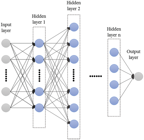
As both algorithms have been described in the two above-mentioned papers, here only essential information is introduced. The proposed BP neural network for retrieving SSWS by S1 EW data has four input parameters, i.e. NRCS of S1 sub-images ${\sigma }_{HH}$, the local incidence angle $\theta$, the trigonometric functions of the azimuthal wind direction $\mathrm{c}\mathrm{o}\mathrm{s}\left(\varphi \right)$ and $\mathrm{c}\mathrm{o}\mathrm{s}\left(2\varphi \right)$. The input parameters are determined according to the well-studied GMF, which is widely used for SSW retrieval by spaceborne SAR data. There are three hidden layers in the neural network, which consist of 6, 8 and 10 nodes, respectively. The sole node in the output layer is the SSWS. The activation function of the hidden layer is “tansig” (hyperbolic tangent function), which can converge quickly. The training function is “traindx” (adaptive learning rate training function). The learning function is “learngdm” (gradient descent momentum learning function) to calculate the change rate of weights and thresholds. The “tansig”, “traindx” and “learngdm” are the Matlab built-in functions, which offer conveniences of building up the network. The performance function is the mean square error (MSE) to measure the training performance of each iteration.

The same as SSWS retrieval, a BP neural network was also used to retrieve the SWH by S1 EW data in HH polarization. There are a total of 23 parameters used as inputs to the network. Among them, 22 parameters are the same as those used in the previously developed CWAVE-type empirical algorithms for ERS/SAR and ENVISAT/ASAR wave mode data, i.e. the mean NRCS ${\sigma }_{HH}$, normalized image variance cvar, and 20 spectral parameters computed from the variance spectrum of a sub-image.

The cvar of each sub-image is computed as follows:

(3) $cvar=\mathrm{v}\mathrm{a}\mathrm{r}\left(\frac{I-⟨I⟩}{⟨I⟩}\right)$(3)

where $⟨I⟩$ is mean of the image intensity $I$ of a S1 sub-image. The 20 spectral parameters are extracted from the SAR image spectrum using a set of orthonormal functions, which present features of image spectrum from 20 different direction in wavenumber domains.

As the incidence angle of the S1 EW varies between 18.9° and 47.0°, it has a significant impact on radar backscatter and therefore, it is also included as a critical input parameter. After the multiple trials of using different expressions of incidence angle to train the BP neural network, it is found that the best retrievals can be achieved by using $cos\theta$ as an input to the network. Thus, 23 parameters are collected as the input vector, denoted as X, to the proposed BP neural network.

(4) $X={\left({\sigma }_{HH},cvar,cos\theta ,S_1,\dots ,S_{20}\right)}^T$(4)

As the input parameters to the BP neural network for retrieving SWH by S1 data are much more than those used in the network for SSWS retrieval, more hidden layers (four layers) and nodes are used. The numbers of nodes in the four hidden layers are 30, 20, 10, and 5, respectively. The activation function of the second hidden layer is “logsig” (sigmoid function), and the activation function of the other hidden layers is “tansig”. The training function of the proposed BP neural network is “trainbfgs” (BGFS quasi-Newton method) to avoid computing the second derivative and the inverse of the Hesse matrix to increase the computational efficiency.

In our previous studies on developing the methods to retrieve SSWS and SWH by S1 EW data, preliminary validation with different reference data was carried out, as summarized in Table 1. Regarding the validation of S1-retrieved SSWS, the RMSE is overall less than 1.50 m/s comparing with three different reference datasets and the bias achieves the lowest value of 0.09 m/s by comparing with in situ buoy measurements. In addition to comparing the S1-retrieved SWH with multiple RA data, we also compared them with measurements from the Surface Waves Investigation and Monitoring (SWIM) sensor (a real aperture radar) onboard the Chinese French Oceanic SATellite (CFOSAT). Both comparisons present a similar RMSE of approximately 0.60 m. Based on stable performances of the S1-retrieved SSWS and SWH, we further applied the proposed BP neural network methods to more S1 EW data acquired during the period January 2017 through May 2021.

4. Data records

During this period, we processed a total of 54,172 S1 EW images to retrieve SSW and SWH based on the proposed BP neural network methods. Only the S1 EW images in which the sea ice cover less than 85% (determined by the AMSR2 sea ice concentration data) were used to retrieve SSWS and SWH. To better prompt the application of the SAR-retrieved ocean wind and wave data in high spatial resolution, we designed the data records in NetCDF-4 format, following the Climate and Forecast Metadata CF-1.7 convention.

The naming convention of the S1-retrieved wind and wave products is as follows:

Type_Satid_ImaMode_SourTypeRes_ImaDateImaTime_Flag_Ver.nc, where

a. Type: type of product, SWH or SSW

b. Satid: mission name, S1A or S1B

c. ImaMode: SAR imaging mode

d. SourType: type of source product, GRD

e. Res: spatial resolution of source product

f. ImaDate: date of SAR data acquisition

g. ImaTime: time of SAR data acquisition

h. Flag: sole flag of source product

i. Ver: version of processing software

Each record of SSW and SWH products consists of 8 and 7 variables, respectively, which is listed in Table 4.

Table 4. List of variables and their descriptions in the S1 SSW and SWH products.

No.	Variables	Description
1	Latitude	Latitude at Wind/Wave Cell Center
2	Longitude	Longitude at Wind/Wave Cell Center
3	WindSpeed	SAR Retrieved Sea Surface Wind Speed
4	WindDirection	Interpolated Sea Surface Wind Direction of ERA5 Reanalysis Model (clockwise relative to North)
5	SWH	S1 Retrieved Significant Wave Height
6	IncidenceAngle	Incidence Angle at Wind/Wave Cell Center
7	Sigma0	Normalized Radar Cross Section
8	Mask	0 for acceptable S1 sub-images for retrieval 1 for inhomogeneous S1 sub-images 2 for ice-covered S1 sub-images 3 for land-covered S1 sub-images
9	qc_flag	0 for a good record 1 for a suspect record 2 for a bad record 3 for an unprocessed record

The “WindSpeed” refers to the S1-retrieved SSWS at 10 m height. The ERA5 wind direction (coming from) is stored as the variable “WindDirection”, which is interpolated to 2 km × 2 km, the same size as S1 sub-images used for retrieval.

The “SWH” is the S1-retrieved SWH.

The “Mask” flag marks the S1 sub-images with values of 0, 1, 2 or 3, which represents an acceptable S1 sub-image for retrieval, an inhomogeneous sub-image (homogeneity factor > 1.05), a record containing ice, and a record containing land. The ice-covered and land-covered areas are extracted by IMS data (which applies the GSHHS data for land mask).

The “qc_flag” variable can have four values that describe the quality of the retrieved SSWS or SWH data. For the SSW data, the different qc_flag records (Table 5) satisfy the following criteria.

Table 5. Definition of quality control flags and their criteria for the SSW products.

Record	Criteria
Good record (qc_flag = 0)	a. 0 m/s < SSW < 30 m/s and b. homogeneity factor ≤ 1.05
Suspect record (qc_flag = 1)	a. SSW > 30 m/s or b. 1.05 < homogeneity factor ≤ 1.50
Bad record (qc_flag = 2)	a. SSW < 0 m/s or b. 1.50 < homogeneity factor ≤ 3.00
Unprocessed record (qc_flag = 3)	a. Mask = 2 or Mask = 3 or b. homogeneity factor > 3.00

As described in Section 3, the homogeneity factor is a crucial quality control parameter of SSW retrievals. Additionally, considering the data range of training and testing datasets, the accuracy of the retrieved SSWS higher than 30 m/s is hard to validate. Therefore, when both the homogeneity factor of an S1 sub-image≤1.05 and the corresponding retrieved SSW are less than 30 m/s, the records are considered “good”. The retrieved SSWS is considered as “suspect record” if it is higher than 30 m/s. We also found that some of the retrievals by S1 sub-images with homogeneity factors no larger than 1.50 are acceptable, which is explained at length in the next Section based on comprehensive validation experiments. For the retrieved SSWS beyond the valid range (i.e. less than 0 m/s) or the homogeneity factor larger than 1.50, the retrievals are flagged as “bad” records. If the S1 sub-images are masked “sea ice cover” or “land” or with the homogeneity factor larger than 3.0, they are not processed for retrievals.

For the S1-retrieved SWH product, the defined quality control flags are summarized in Table 6. The valid range of SWH retrievals and homogeneity factor are two key flags, similar to those used in the flags for SSW products. Besides, normalized equivalent sigma zero (NESZ, i.e. the noise floor of the SAR data) and normalized image variance (defined in Eq.(3(3) $cvar=\mathrm{v}\mathrm{a}\mathrm{r}\left(\frac{I-⟨I⟩}{⟨I⟩}\right)$(3) )) parameters are used. If the difference between the mean NRCS of the S1 sub-images ($\overline{{\sigma }_0}$) and NESZ is less than 3 dB, indicating very low radar backscatter from sea surface and retrievals are significantly biased; therefore, the retrievals are flagged as “bad” records. This flag is also previously used for the ten-year ASAR ocean wave products (Li & Huang, 2020), which has proven effective in filtering low quality data .

Table 6. Definition of quality control flags and their criteria for the SWH products.

Record	Criteria
Good record (qc_flag = 0)	a. 0 m ≤ SWH ≤ 10 m and b. homogeneity factor ≤ 1.05 and c. $\overline{{\sigma }_0}$ – NESZ ≥ 3 dB and d. image variance ≤ 0.25
Suspect record (qc_flag = 1)	a. SWH > 10 m or b. 1.05 < homogeneity factor ≤ 1.50 and c. $\overline{{\sigma }_0}$ – NESZ ≥ 3 dB and d. image variance ≤ 0.25
Bad record (qc_flag = 2)	a. SWH < 0 m or b. 1.50 < homogeneity factor ≤ 3.00 or c. $\overline{{\sigma }_0}$ – NESZ < 3 dB or d. 0.25 < image variance ≤ 0.50
Unprocessed record (qc_flag = 3)	a. Mask = 2 or Mask = 3 or b. homogeneity factor > 3.00 or c. image variance > 0.50

The thresholds of image variance as quality control flag for good, bad records are 0.25 and 0.5, respectively, which are also determined based on the validation experiment introduced in the following section.

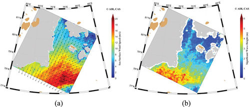
The S1-retrieved wind and wave products are not only provided with NetCDF files, but also with thematic maps in JPEG format, as a case shown in Figure 5. In the maps, the gray represents sea ice cover.

Figure 5. Examples of (a) SSW and (b) SWH products produced by S1 EW data acquired in the Arctic. the gray represents areas covered by sea ice. the image ID is S1A_EW_GRDM_1SDH_20201202T024920_20201202T025025_035501_042682_F0C5.

5. Technical validation

A comprehensive validation by comparing the S1-retrieved wind and wave data with collocated ASCAT and RA data was conducted. To compare the SSWS data, we limited the valid range from 0 m/s to 30 m/s. The temporal window and spatial distance of collocating ASCAT and S1-retrieved SSWS are 60 min and 25 km, respectively. The collocations of S1 retrievals with RA data are also limited to 60 min, while the spatial distance depends on the footprint size of each altimeter mission.

5.1. Validation of the S1-retrieved SSWS

The ASCAT wind data are available in a cell with the size of 25 km × 25 km. Therefore, all the S1-retrieved SSWS in grids with a size of 2 km × 2 km within a collocated ASCAT wind cell are averaged for comparison. Based on the above-mentioned collocation criteria, we eventually extracted 832,256 data pairs during the period from June 2018 to June 2020. Similar to collocation with ASCAT data, all the S1-retrieved SSW data within a footprint of RA are averaged for comparison, which yield a total of 68,924 data pairs during this period.

It is mentioned in the Section 3 of Data Records that we determined the flags of homogeneity for “suspect” and “bad” records based on the comparisons with ASCAT and RA wind data. Here are explained in detail. Table 7 lists the achieved statistical parameters for comparisons with ASCAT and RA SSWS data in different ranges of homogeneity factor. Among the S1 collocations with ASCAT data, there are 97.2% of data pairs with homogeneity factors ≤ 1.05. For the S1 data collocated with RA data, there are 95.4% with homogeneity factors ≤ 1.05. The comparisons in this range of homogeneity factor suggest the S1-retrieved SSWS is in good consistency with ASCAT and RA wind data, with RMSE of approximately 1.50 m/s, SI of 17% and a high correlation of 0.94.

Table 7. Comparisons of SSWS by S1 with ASCAT/RA data for different homogeneity factors.

Homogeneity factor	Comparing data	Counts	Bias (m/s)	RMSE (m/s)	SI (%)	Correlation
≤1.05	ASCAT_SSW	805,851	−0.02	1.45	16.83	0.94
	RA_SSW	65,780	0.61	1.61	17.54	0.94
(1.05, 1.50]	ASCAT_SSW	23,476	0.51	1.54	34.08	0.95
	RA_SSW	2,906	0.47	1.69	35.93	0.94
(1.50, 3.00]	ASCAT_SSW	1,264	0.57	2.44	96.55	0.75
	RA_SSW	238	1.49	4.42	160.68	0.55

For the comparisons with the homogeneity factor between 1.05 and 1.50 (proportion is 2.8% and 4.3% of each collocation dataset, respectively), the RMSE slightly increases (1.54 m/s vs. 1.45 m/s for the comparison with ASCAT and 1.69 m/s vs. 1.61 m/s for the comparison with RA) and correlation remains unchanged. However, the SI is almost two times higher, suggesting that the data pairs of S1 and ASCAT, or S1 and RA are somewhat scattered, which should be caused by retrievals of inhomogeneous S1 sub-images. Therefore, the S1 retrievals with the homogeneity factor between 1.05 and 1.50 are flagged “suspect” records. For the comparisons with higher homogeneity value beyond 1.50, it is found that all the statistical parameters become unacceptable, and therefore, the corresponding retrievals are flagged “bad” or “unprocessed”.

Figure 6(a,b) presents the scatter diagrams of comparisons between S1-retrieved SSWS and the collocated ASCAT and RA data, respectively, with the homogeneity factor≤1.05. The overlaid error bars represent the mean ± standard deviation at an interval of 2 m/s. It is found that there are quite some outliers in the comparisons, which can possibly be induced by temporal and spatial differences between SAR and ASCAT, RA collocations. Therefore, we used quartiles to exclude some outliers, which are widely used to determine the range of outliers in the box plot (Tukey, 1977). The quartiles, $Q_1$, $Q_2$, and $Q_3$, are acquired by splitting data into four equal parts. The first quartile $Q_1$ divide data into the first 25% and the rest 75%, the second quartile $Q_2$ is the median of data, and the third quartile $Q_3$ is the median between the $Q_2$ and the maximum. The interquartile range (denote as $IQR$) is the difference between $Q_3$ and $Q_1$. Using the quartiles and interquartile, the following two boundaries are calculated.

(5) $lowerbound=Q1-1.5IQR$(5)

(6) $upperbound=Q3+1.5IQR$(6)

Figure 6. Comparisons of SSWS by S1 and the collocated (a) ASCAT and (b) RA from June 2018 to June 2020. The gray dots are the detected outliers by quartiles. The color indicates the amount of collocated data pairs. The error bars in an interval of 2 m/s are overlaid.

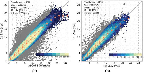
The outliers are defined as the data beyond the two boundaries and are represented by the gray dots in Figure 6. After excluding these outliers, 777,376 pairs collocated with ASCAT data and 62,709 pairs collocated with RA data have eventually remained for validation. For the comparison with ASCAT SSWS data, values of the four statistical parameters are: a correlation of 0.96, a bias of 0.10 m/s, an RMSE of 1.23 m/s and an SI of 14.2%. For the comparison with RA wind speed data, they are: a bias of 0.54 m/s, an RMSE of 1.35 m/s, and an SI of 14.46%, slightly increasing. From the diagrams we can find a few key points: (1) the S1-retrieved SSWS are in good consistency with both ASCAT and RA data; (2) the S1 retrievals are generally higher than the RA data in the range of approximately 4 m/s to 12 m/s, inducing a high bias of 0.54 m/s for the overall comparison because the data amount in this range is in a high proportion of the whole collocation dataset; and (3) the S1 retrievals are underestimated for wind speed larger than 20 m/s and the underestimation seems to increase along with wind speed increase.

In subsection 2.2, the bias achieved in the cross-comparisons of SSWS data from different RA missions shows some fluctuations. It may suggest that there are some discrepancies of the SSWS data among the four RA missions. Therefore, we also conducted separate comparisons of SSWS by S1 with the data from the four RA missions. The results are presented in Table 8. The comparison of S1-retrieved SSWS has the best agreement with the Jason-2 data with a bias of 0.40 m/s and an RMSE of 1.22 m/s. The comparison with SARAL yields the highest RMSE and SI of 1.69 m/s and 14.80%, respectively. This may attribute to two reasons: 1) the SSWS data by SARAL probably have the worst performances among the four RA missions; 2) the quite fewer collocated data pairs compared with collocations with the other three RA missions. The comparisons with CryoSat-2 and Jason-3 data yield comparable data pairs and have very similar performances in terms of all three statistical parameters.

Table 8. Comparisons of the SSWS by S1 and RA from different missions.

RA	No. Col.	Bias (m/s)	RMSE (m/s)	SI (%)
CryoSat-2	21,594	0.68	1.44	12.49
Jason-2	13,268	0.40	1.22	12.10
Jason-3	24,574	0.62	1.41	12.71
SARAL	3,942	0.58	1.69	14.80

5.2. Validation of the S1-retrieved SWH data

First, we also explain the determinations of two quality control flags based on the validation experiment. Among the 68,924 data pairs of S1 and RA, there are 1,384 ones with values of $\overline{{\sigma }_0}$ – NESZ less than 3 dB. Their comparisons with RA SWH yield a bias of 2.6 m, an RMSE of 3.49 m and an SI of 145.05%. On the contrary, the comparison of the data with the value $\overline{{\sigma }_0}$ – NESZ larger than 3 dB yields a bias of 0.26 m, an RMSE of 0.86 m and a SI of 26.52%. This further proves that the determined quality control flag of the difference between mean NRCS and NESZ can effectively filter retrievals in low quality.

Besides, we further checked the retrievals with different combinations of homogeneity factor and image variance. The corresponding statistical parameters of comparisons as listed in Table 9. Indeed, for the S1 sub-images with image variance≤0.25 and homogeneity factor≤1.05 yield retrievals with the best quality compared with other combinations. When the image variance is between 0.25 and 0.5, no matter whether the homogeneity factor is low or not, the retrievals are of poor quality, which suggests that the set of quality control flag of image variance with the threshold of 0.25 is practical.

Table 9. Comparisons of SWH by S1 with RA data with different combinations of homogeneity factor and image variance.

Homogeneity Factor Image variance	Statistical Parameters	≤1.05	(1.05, 1.50]
[0, 0.25]	No. Col.	64,719	815
	Bias (m)	0.23	0.10
	RMSE (m)	0.76	1.18
	SI (%)	26.36	48.59
	Correlation	0.89	0.67
(0.25, 0.50]	No. Col.	2092	18
	Bias (m)	0.81	0.50
	RMSE (m)	1.93	3.26
	SI (%)	95.00	122.40
	Correlation	0.38	0.03

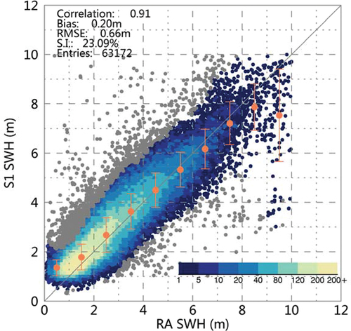
Figure 7 shows the scatter diagram of the comparison of S1-retrieved SWH with “qc_flag” of “good” with the collocated RA data. We also used quartiles to exclude some outliers, and finally, 63,172 data pairs remained. The error bar represents the mean and standard deviation of retrieved SWH in every interval of 1 m of RA SWH. The comparison excluding the outliers yields a correlation of 0.91, a bias of 0.20 m, an RMSE of 0.66, and an SI of 23.09%, indicating a good agreement between S1 retrievals and RA data. However, similar to the comparison of SSWS presenting underestimation under high winds, the S1-retrieved SWH also tends to underestimate the sea state for SWH higher than 8 m.

Figure 7. Comparison of SWH by S1 and the collocated RA during the period of June 2018 to June 2020. the gray dots are the outliers detected by quartiles. the color indicates the amount of collocated data pairs.

6. Usage notes

6.1. Recommended software tool for quick view of the dataset

The Panoply Data Viewer developed by the US National Aeronautics and Space Administration (NASA) Goddard Institute for space studies is freely available for a quick view of the developed S1 sea surface wind and ocean wave products in NetCDF format. For more information about the software, please refer to: https://www.giss.nasa.gov/tools/panoply/.

6.2. Developed program for dataset processing

We also developed a MATLAB-based program for reading a single wind and wave product in the NetCDF format. It is shared together with the dataset available at Science Data Bank.

7. Potential applications

The Arctic ocean has never been paid so much attention to not only by scientific community but also by government and industry stakeholders. The developed ocean wind and wave data in high spatial resolution and wide coverage by spaceborne SAR in the Arctic Ocean can significantly contribute to studies on interaction between sea ice and ocean dynamics (and possible consequent feedback to sea ice decline) and interactions between ocean dynamics and coast (e.g. frozen soil). On the other hand, in practical, they can provide key support for offshore construction and shipping safety and security in the passages in the Arctic. We are processing the historical S1 data and will continue to process the ongoing acquired data. After accumulating for a long time, we believe such a valuable dataset can contribute to stuidies on wind and wave climate in the Arctic ocean for better understanding the changing Arctic.

Disclosure statement

No potential conflict of interest was reported by the author(s).

Data availability statement

This dataset is freely available at Science Data Bank http://www.dx.doi.org/10.11922/sciencedb.00834.

Additional information

Funding

The study was partially supported by the National Key Research and Development Program of China [2018YFC1407100] and the National Science Fund for Distinguished Young Scholars [42025605].

Notes on contributors

Xiao-Ming Li

Xiao-Ming Li received his Ph.D. degrees in Geophysics and Marine Remote Sensing, from the University of Hamburg, Hamburg, Germany and Ocean University of China, Qingdao, China, in 2010, respectively. From June 2006 to January 2010, he was a research assistant with the German Aerospace Center (DLR) in Oberpfaffenhofen; afterward, he continued to work at DLR as a research scientist till January 2014. Since February 2014, he has been a full professor in the Institute of Remote Sensing and Digital Earth and now the Aerospace Information Research Institute, Chinese Academy of Sciences. His research interest is spaceborne SAR oceanography.

Ke Wu

Ke Wu received her master degree in 2021 from the University of Chinese Academy of Sciences. She is now pursuing a Ph.D. degree at the Aerospace Information Research Institute, Chinese Academy of Sciences. She majors in satellite ocean remote sensing and her research interests include SAR retrievals of ocean dynamic parameters and machine learning.

Bingqing Huang

Bingqing Huang received her master degree in 2017 from Ocean University of China. She is now pursuing a Ph.D. degree at Aerospace Information Research Institute, Chinese Academy of Sciences. She majors in satellite ocean remote sensing and her research interests include retrieving ocean dynamic parameters from SAR and the interaction between sea-ice and ocean waves.

References

- Ali, M. M., Bhat, G. S., Long, D. G., Bharadwaj, S., & Bourassa, M. A. (2013). Estimating wind stress at the ocean surface from scatterometer observations. IEEE Geoscience and Remote Sensing Letters, 10(5), 1129–1132.
- Alpers, W. R., Ross, D. B., & Rufenach, C. L. (1981). On the detectability of ocean surface waves by real and synthetic aperture radar. Journal of Geophysical Research, 86(C7), C7.
- Ardhuin, F., Chapron, B., & Collard, F. (2009). Observation of swell dissipation across oceans. Geophysical Research Letters, 36(6), L06607.
- Asplin, M. G., Galley, R., Barber, D. G., & Prinsenberg, S. (2012). Fracture of summer perennial sea ice by ocean swell as a result of Arctic storms. Journal of Geophysical Research: Oceans, 117(C6), C6.
- ESA (European Space Agency). (2016). Sentinel-1 product specification. (Retrieved October 5, 2020). https://sentinel.esa.int/web/sentinel/document-library/content/-/article/sentinel-1-product-specification
- Hasselmann, S., Brüning, C., Hasselmann, K., & Heimbach, P. (1996). An improved algorithm for the retrieval of ocean wave spectra from synthetic aperture radar image spectra. Journal of Geophysical Research: Oceans, 101(C7), 16615–16629.
- Helfrich, S. R., Li, M., Kongoli, C., Nagdimunov, L., & Rodriguez., E. (2019). Interactive multisensor snow and ice mapping system version 3 (IMS V3) - algorithm theoretical basis document version 2.5. NOAA NESDIS Center for Satellite Applications and Research (STAR), 74.
- Hersbach, H., Bell, B., Berrisford, P., Hirahara, S., Horányi, A., Muñoz-Sabater, J., & Thépaut, J. (2020). The Era5 Global Reanalysis. Quarterly Journal of the Royal Meteorological Society doi:https://doi.org/10.1002/qj.3803
- Huang, W., Gill, E. W., Wen, B., Wen, B., & Hou, J. (2002). Hf radar wave and wind measurement over the eastern China sea. IEEE Transactions on Geoscience and Remote Sensing, 40(9), 1950.
- Huang, W., Liu, X., & Gill, E. W. (2017). Ocean wind and wave measurements using x-band marine radar: A comprehensive review. Remote Sensing, 9(12), 1261.
- Inoue, J., Yamazaki, A., Ono, J., Dethloff, K., Maturilli, M., Neuber, R., & Yamaguchi, H. (2015). Additional arctic Observations Improve Weather and Sea-ice Forecasts for the Northern Sea Route. Scientific Reports, 5, 16868.
- Khan, S. S., Echevarria, E. R., & Hemer, M. A. (2021). Journal of Geophysical Research: Oceans. Ocean Swell Comparisons between Sentinel-1 and WAVEWATCH III around Australia, 126, e2020JC016265.
- Kodaira, T., Waseda, T., Nose, T., Sato, K., Babanin, A., Voermans, J., & Babanin, A. (2021). Observation of on-ice wind waves under grease ice in the western Arctic ocean. Polar Science, 27(96), 100567.
- Leigh, S., Wang, Z., & Clausi, D. A. (2014). Automated ice-water classification using dual polarization sar satellite imagery. IEEE Transactions on Geoscience and Remote Sensing, 52(9), 5529–5539.
- Li, S., Shen, H., Hou, Y., He, Y., & Bi, F. (2018). Sea surface wind speed and sea state retrievals from dual-frequency altimeter and its preliminary application in global view of wind-sea and swell distributions. International Journal of Remote Sensing, 39(10), 3076–3093.
- Li, X.-M. (2016). A new insight from space into swell propagation and crossing in the global oceans. Geophysical Research Letters, 43(10), 5202–5209.
- Li, X. M., ., & Huang, B. Q. (2020). A global sea state data set from spaceborne synthetic aperture radar wave mode data. Scientific Data, 7(1), 261.
- Li, X. M., & Lehner, S. (2013). Observation of terrasar-x for studies on offshore wind turbine wake in near and far fields. IEEE Journal of Selected Topics in Applied Earth Observations & Remote Sensing, 6(3), 1757–1768.
- Li, X.-M., Lehner, S., & Bruns, T. (2011). Ocean wave integral parameter measurements using Envisat ASAR wave mode data. IEEE Transactions on Geoscience and Remote Sensing, 49(1), 155–174.
- Li, X. M., Qin, T. T., & Wu, K. (2020). Retrieval of sea surface wind speed from spaceborne SAR over the Arctic marginal ice zone with a neural network. Remote Sensing, 12, 20.
- Li, X.-M., Sun, Y., & Zhang, Q. (2021). Extraction of sea ice cover by Sentinel-1 SAR based on support vector machine with unsupervised generation of training data. IEEE Transactions on Geoscience and Remote Sensing, 1–14. doi:https://doi.org/10.1109/TGRS.2020.3007789
- Ozbahceci, B. O. (2020). Extreme value statistics of wind speed and wave height of the Marmara sea based on combined radar altimeter data. Advances in Space Research, 66(10), 2302–2318.
- Podgórski, K., & Rychlik, I. (2014). A model of significant wave height for reliability assessment of a ship. Journal of Marine Systems, 130, 109–123.
- Ribal, A., & Young, I. R. (2019). 33 years of globally calibrated wave height and wind speed data based on altimeter observations. Scientific Data, 6, 1–15.
- Rubio, A., Mader, J., Corgnati, L., Mantovani, C., Griffa, A., Novellino, A., & Puillat, I. (2017). radar activity in European coastal seas: Next steps toward a pan-European HF radar network. Frontiers in Marine Science, 4, 8.
- Schulz-Stellenfleth, J., König, T., & Lehner, S. (2007). An empirical approach for the retrieval of integral ocean wave parameters from synthetic aperture radar data. Journal of Geophysical Research, 112(C3), C3.
- Schulz-Stellenfleth, J., & Lehner, S. (2004). Measurement of 2-D Sea Surface Elevation Fields Using Complex Synthetic Aperture Radar Data. IEEE Transactions on Geoscience and Remote Sensing, 42(6), 1149–1160.
- Stoffelen, A., & Anderson, D. (1997). Scatterometer data interpretation: Estimation and validation of the transfer function CMOD4. Journal of Geophysical Research Oceans, 102(C3), 5767–5780.
- Stopa, J. E., Ardhuin, F., Thomson, J., Smith, M. M., Kohout, A., Doble, M., Wadhams, P. (2018). Wave attenuation through an Arctic marginal ice zone on 12 October 2015: 1. measurement of wave spectra and ice features from sentinel 1A. Journal of Geophysical Research: Oceans, 123(5), 3619–3634.
- Stopa, J. E., & Mouche, A. (2017). Significant wave heights from Sentinel-1 SAR: Validation and applications. Journal of Geophysical Research: Oceans, 122(3), 1827–1848.
- Thompson, D. R., & Beal, R. C. (2000). Mapping high-resolution wind fields using synthetic aperture radar. Johns Hopkins University Technical Digest, 273(5279), 1181–1182.
- Tukey, J. (1977). Exploratory Data Analysis. Addison-Wesley Publishing Company, Reading, Massachusetts.
- Wang, Y., & Li, X.-M. (2021). Arctic sea ice cover data in high spatial resolution from spaceborne synthetic aperture radar by deep learning. Earth System Science Data, 13(6), 2723–2742.
- Waseda, T., Webb, A., Sato, K., Inoue, J., Kohout, A., Penrose, B., & Penros, S. (2018). Correlated increase of high ocean waves and winds in the ice-free waters of the arctic ocean. Scientific Reports, 8(1), 4489.
- Wu, K., Li, X.-M., & Huang, B. Q. (2021). Retrieval of ocean wave heights from spaceborne sar in the arctic ocean with a neural network. Journal of Geophysical Research: Oceans, 126(3). doi:https://doi.org/10.1029/2020JC016946
- Young, I. R., Zieger, S., & Babanin., A. V. (2011). Global trends in wind speed and wave height. Science, 332(6028), 451–455.