GIScience research challenges for realizing discrete global grid systems as a Digital Earth

ABSTRACT

Increasing data resources are available for documenting and detecting changes in environmental, ecological, and socioeconomic processes. Currently, data are distributed across a wide variety of sources (e.g. data silos) and published in a variety of formats, scales, and semantic representations. A key issue, therefore, in building systems that can realize a vision of earth system monitoring remains data integration. Discrete global grid systems (DGGSs) have emerged as a key technology that can provide a common multi-resolution spatial fabric in support of Digital Earth monitoring. However, DGGSs remain in their infancy with many technical, conceptual, and operational challenges. With renewed interest in DGGS brought on by a recently proposed standard, the demands of big data, and growing needs for monitoring environmental changes across a variety of scales, we seek to highlight current challenges that we see as central to moving the field(s) and technologies of DGGS forward. For each of the identified challenges, we illustrate the issue and provide a potential solution using a reference DGGS implementation. Through articulation of these challenges, we hope to identify a clear research agenda, expand the DGGS research footprint, and provide some ideas for moving forward towards a scaleable Digital Earth vision. Addressing such challenges helps the GIScience research community to achieve the real benefits of DGGS and provides DGGS an opportunity to play a role in the next generation of GIS.

KEYWORDS:

• DGGS
• discrete global grid systems
• GIScience
• Digital Earth

1. Introduction

The necessity of local adaptation to global change remains one of the hallmarks of the 21st century. Global climate change is causing glaciers to retreat, shifts in plant and animal distributions, changes in plant phenology, sea level rise, intense heat waves, and more severe wildfire seasons. As governments and communities adapt to these changes, there is increased need to integrate a wide variety of environmental information sources. Coincident with this growing demand for geospatial earth observation data has been the development of Digital Earth technologies aiming to address some of these information needs (Craglia et al., 2012). Digital Earth platforms are proposed as tools to provide data integration, modeling, and an observation system to manage environmental changes at different geographic scales (Craglia et al., 2012). Discrete global grid systems (DGGSs) have been proposed as a spatial data model to support the Digital Earth vision. A DGGS has many advantages over traditional raster and vector data models (Lewis, 2017; Purss et al., 2019) and is thus being actively developed in the academic literature (e.g. Mahdavi Amiri, Alderson, & Samavati, 2019; Sahr, White, & Kimerling, 2003; Sherlock, Tripathi, & Samavati, 2016; Shuang, Cheng, Chen, & Meng, 2016; Sirdeshmukh, Verbree, Van Oosterom, Psomadaki, & Kodde, 2019; Tripathi, Sherlock, Amiri, & Samavati, 2016) and industry (e.g. Uber, 2020) and via international organizations such as the Open Geospatial Consortium (e.g. Gibb, Cochrane, & Purss, 2021).

Despite this renewed research and commercial interest in DGGS, participation of the GIScience community in DGGS remains focused on a relatively narrow set of questions stemming from grid specification and refinement (e.g. Sahr, 2019; Sahr et al., 2003; Ulmer, Hall, & Samavati, 2020; Wang, Ben, Zhou, & Zheng, 2020), on the one hand, and broader papers outlining DGGS visions and potential, on the other hand (see Purss et al., 2019). Given the current availability and maturity of software for DGGS grid generation (e.g. DGGRID, H3, Pyxis, and rHEALPix), we believe that the time is right for more expansive technical and methodological GIScience research engaging with DGGS. Through the development of a DGGS-based environmental analytics platform in support of a program of research aiming to link citizen and science perspectives on water in Canada (Robertson, Chiranjib, Majid, & Roberts, 2020), we have identified several GIScience research challenges, which we perceive as barriers to greater DGGS adoption and need further research. Several other recent papers have focused on research challenges related to DGGS. Yao et al. (2020) describe DGGS opportunities and challenges from an architecture perspective, highlighting issues such as grid coding and space-time data specific to implementation in a cloud environment. Li and Stefanakis (2020b) describe how a set of common algorithms required by the OGC Abstract Specification can be used as building blocks to support extended operations. These authors identified interoperability, basic algorithm development, and data modelling and storage architecture as key areas for future research. In this paper, we focus on identifying and illustrating core GIScience research challenges that can help to move the field(s) of DGGS forward. The main contribution of the authors in this paper is to discuss some of the shortcomings of the current DGGS models and examine some potential solutions that exist to promote greater adoption for Digital Earth applications.

2. GIScience research challenges

In this section, we first discuss broader GIScience challenges existing for using DGGS as an implementation of Digital Earth (subsections 2.1, 2.2 and 2.3). At the end of this section, we discuss some more technical aspects of implementing DGGS from a GISystems view (subsections 2.4 and 2.5).

2.1. Geographic knowledge representation

Human perception and understanding of the environment forms the basis of how we model and interact with geospatial information within GIS. Thus, to some extent, ideas of the geographic world encoded into spatial data models are culturally constructed and/or dependent. This process of perceiving and making meaning of space involves a series of concepts and categories that divide the world into objects, processes, and relationships in different ways (Smith & Mark, 2001). This conceptualization of the world is codified externally by language, toponyms, geographic concepts, etc., which are encoded in a digital representation into the finite set of data models. A data model defines types of data objects and a framework for organizing them (Yuan, 2020). Each data model consists of three main components: i) a set of object types defining basic building blocks, ii) a set of operations providing a means for manipulation of object types, and iii) a set of integrity rules, which constrain the valid state of the data model (Date, 1983).

For hundreds of years, human conceptualization of space was encoded into paper maps, and these in part acted to reinforce our own perception of space. As mapping technology moved to computer systems in the latter half of the 20th century, these nascent GIS were modelled as digital versions of their paper analogues, even replicating ideas of thematic layering of discretely categorized phenomena that inventory selected components of the environment were common in traditional mapping for resource management and navigation. As such, many users of GIS today see the world as an assemblage of discrete layers; however, traditional pre-computerized conceptualizations of space may bare little resemblance to this worldview (Murrieta-Flores, Favila-vtimes New Romanã¡zquez, & Flores-morã¡n, 2019). There may be opportunities for DGGS to address longstanding issues in geographic knowledge representation in GIS (Craglia et al., 2012). The nature of the multi-resolution grid structure that DGGS provides helps to address challenges such as geoprivacy, uncertainty, and large-scale analysis. However, a fundamental aspect of using DGGS as a data model is to represent geographic information as a set of discrete cells. It is important to see the DGGS as a framework not as a data storage or indexing structure for cells.

Despite widespread adoption of raster and vector geographic data models, there have been numerous proposals that aimed to provide an alternate representation of geographic phenomena. For example, Barnsley, Møller-Jensen, and Barr (2001) identifies the challenges in semantics of the definition of land use and land cover in urban areas and defines object-based geographic representation. In their data model as a knowledge-based texture method, they identify parameters including object name, object parent, code, size, colour, and shape. The topological relations between the objects in this model are defined as graph edges. A similar graph representation of the geographic information has been proposed by Bouille (1978), which aimed to encapsulate the topological relation and complexities within geographic information. They emphasize that the data structure should not be confused with the storage and retrieval methods. In their HyperGraph data model, they identify items such as class, object, relation, and attribute, each data set includes a set of classes, and each class has a set of objects and relations. Similar graph-based models have been developed by Zhang and Gong (2002), and Roberts, Hall, and Calamai (2011) used explicit primal and dual graph representation to apply multi-objective optimization methodologies to a an environmental design problem.

The most common representations of geographic information are based on the categorization of space as field data and object data, which are realized through vector and raster spatial data models, respectively. For field data (continuous data), the raster data model and later data cubes (see Appel & Pebesma, 2019) have been mainly used by mainstream geographic analysis of spatial environmental data. Most of the proposed data models to represent geographic information have tried to address complex topologies and address the crisp boundary issues (e.g. Clementini & Di Felice, 1996) in vector data.

The current representation of geographic information using OGC’s simple feature standards raises other issues related to the semantics of the data. Take Briggs et al. (2020) as an example, which discusses the difference between place and space. The definition of place is often described as location with meaning, while in the context of geospatial data and technologies, the sense of place is reduced to space only (Briggs et al., 2020; Quesnot & Roche, 2015). In a broader context, many Indigenous forms of place-based knowledge is characterized as holistic, experiential, and oral, in contrast to Eurocentric knowledge, which is characterized as quantitative, objective, and written (Briggs et al., 2020; Rundstrom, 1995). Decades of GIScience research have developed sharp critique and a variety of alternatives, which consider the cultural and social aspects (place) using methods to represent space other than simple features (i.e. point, line, and polygon). In Public Participatory GIS (PPGIS) initiatives, broad and representative community participation can be hindered when existing representations of geographic objects fail to adequately capture community geographic knowledge (Tim, Walker, & Mor, 2019). Finally, many forms of community-held knowledge are shared via social and/or community relationships. Sensitive knowledge like sacred sites, practices, etc. require different levels of access and accuracy in data representation, which can be embedded in the data model (Gumbula, 2005).

The limitations of the field and object spatial data models create an opportunity for DGGS, which may provide a more flexible representation of space and encode topological relationships such as neighborhood and hierarchical structures more efficiently. For example, in the raster data model, the use of equal size pixels for large areas introduces distortions in higher latitudes (for example, MODIS images), which can be addressed by using equal area grid systems. Furthermore, the representation of uncertainty in the geometry and embedding different geoprivacy levels into the geographic information are other examples that DGGS is able to address, that is, the extent of the cell can be interpreted to model the extent of positional uncertainty (or at least a class of positional uncertainty) (for example, see Hojati, Farmer, Feick, & Robertson, 2021; Hojati, Robertson, & Feick, 2019).

2.1.1. Object data representation in DGGS

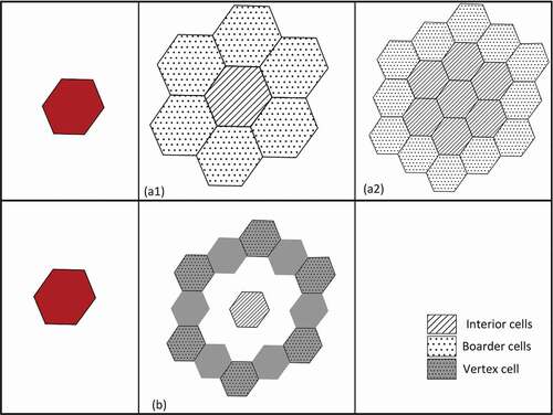
There have been several data models developed on top of the DGGS grid in order to implement geometries such as point, line, and polygon objects. For example, Sirdeshmukh et al. (2019) proposed a 3D data model to represent point cloud data. Similar efforts have been made by Tong, Ben, Liu, and Zhang (2013) to create a vector expression on planar and DGGS grids for line and area objects. Their model covers storage of boundary cells of the area, and for the lines, they have developed a cell-to-cell line drawing algorithm. Their line-filling and area-filling algorithms are the basis of data recording and data expression. Robertson et al. (2020) also proposed a geometric representation of geographic objects as an array of cells. In order to represent the geometry of each geographic feature, there are two main methods. First, it can be addressed by nested subsets of DGGS cells. In this method, each geographic feature is stored as an array of cells. Each cell also stores a set of metadata in order to store topology relations of geographic information. Figure 1(a–c) show the representation method for point, line, and polygon geometries.

Figure 1. Two methods of geographic object representation in the DGGS model. (a–c) Cell subset method and (d–e) Vertex cell subset. (a) point objects, (b) and (d) line objects, and (c) and (e) polygon objects.

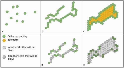
Another method to represent geographic objects is based on the storage of vertices as cell ID and later using algorithms such as Bresenham’s algorithm (Bresenham, 1965) or Tong’s algorithms (Tong et al., 2013) in order to fill between the vertex cells (Figure 1(d-e)). Table 1 shows the necessary metadata for each cell for each method. In the first method for the point data, only accessing the unique cell ID is enough. For the linear method, an ordered array of the cell IDs is required. The order of cells is a representation of the line direction. For polygon objects, two arrays are required, one ordered array of the boundary cells and one array of interior cells. Since the entire array of cells per each feature is available in this representation, geometric functions can be performed using set theory functions. In the second method of geographic object representation, having an ordered array of vertices of a geographic objects vector is enough for calculation of filling cells. However, in this case for geometric operations like buffering or intersections, filling between the stored cells will entail more complex geometric algorithms.

Table 1. Required metadata for different types of geographic model representations.

Method	Traditional model	DGGS-Based Model
Cell subset	Point	Only attributes
(Method 1)	Line	Attributes – order of cells
	Polygon	Attributes – order of cells – border cells – interior cells
	Raster Band	Value
Vertex cell subset
(Method 2)	Point	Only attributes
	Line	Order of cells
	Polygon	Order of cells
	Raster Band	Value

2.1.2. Field data representation in DGGS

Representation of field data can be done by storing each pixel in the raster as a DGGS cell. However, for raster data with large spatial coverage, an optimal resolution should be selected.

Each of the above methods require additional indexing methods in order to perform geometric functions, and this will directly affect the performance of the functions. As a result, defining a standard data model for representation of all geographic objects and its related metadata for DGGS interoperability is necessary. The OGC has recently developed standards for DGGS API for this purpose (Gibb et al., 2021). In their standard, a quantization service is defined as a set of tools to convert non-DGGS spatial data to a DGGS representation. In the OGC standard DGGS, geometry types are defined as OrdinateList for point data, DirectedOrdinateList as a line data, and CellList as the polygon data (Table 32 and 33 in Gibb et al., 2021). This standard covers the definition of different geometry types using DGGS cell IDs.

Earth-observation sensor platforms and providers are increasingly developing analysis-ready data for large-scale data and ongoing change detection and monitoring. A DGGS data model is able to provide a flexible structure for analysis; however, different quantizations for the geometries are not scaleable. For example, quantization of a polygon with an area of $100k{m}^2$ for the resolution of 20 of DGGRID (Sahr et al., 2003) has approximately 6,835 cells, if we follow the OGC geometry model. The number of cells can increase quickly and requires large computational resources. It can be argued that the correct choice of DGGS resolution can address such a problem but considering the role of the current Digital Earth movement, which is aiming more global scales than local, the accessibility of models for local communities that usually do not have enough resources to do so will be limited. Another solution would be exploiting the variable resolution structure of DGGS to approximate homogeneous areas with larger cells. However, this approach introduced additional challenges of parent/child nesting and requires development of quick geographic object conversions methods from one resolution to another and multi-resolution analysis.

2.1.3. Topological issues with DGGS

For vector spatial data, a model of topological spatial relationships is given by the 9-intersection model (Egenhofer & Herring, 1990) or extended 9-intersection model (Section 2.2.13.2 in OGC, 1999). The latter of which includes a dimension of the intersection relationships.

In both cases, areal objects are split into 3 components. For an object $A$, the interior is designated $A^0$, the boundary $\mathrm{\partial }A$, and the exterior $A^{-}$. The 9-intersection model may be represented in a binary matrix as below:

$\left(\begin{array}{ccc}{A}^0\cap B^0& A^0\cap \mathrm{\partial }B& A^0\cap B^{-}\\ \mathrm{\partial }A\cap B^0& \mathrm{\partial }A\cap \mathrm{\partial }B& \mathrm{\partial }A\cap B^{-}\\ A^{-}\cap B^0& A^{-}\cap \mathrm{\partial }B& A^{-}\cap B^{-}\end{array}\right)$

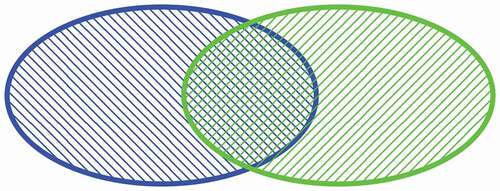
For example, for two areal regions, $A$ and $B$, the overlap relation looks as follows visually (Figure 2) and as a binary matrix (below), where TRUE values are represented as 1s and FALSE values as 0s.

Figure 2. Overlap relation for two areal regions A and B in the traditional vector model.

$\left(\begin{array}{ccc}1& 1& 1\\ 1& 1& 1\\ 1& 1& 1\end{array}\right)$

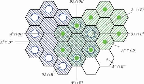
If we now consider the vector-like DGGS representation, where for extended areal features, we distinguish between interior and boundary cells and by extension exterior cells, then we can consider an example of an overlap topological relation between two DGGS features $A$ and $B$, both visually (Figure 3) and via the binary intersection matrix,

Figure 3. Overlap topological relation between two DGGS features $A$ and $B$ for the standard topological model.

$\left(\begin{array}{ccc}1& 1& 1\\ 1& 1& 1\\ 1& 1& 1\end{array}\right)$

But note that we can also have an overlap case as follows (see Figure 4), which does not exist in the standard or extended 9-intersection topological model. Here, we do not have the relationship $A^{-}\cap B^0$. It turns out that we need to turn to an expanded model designed for broad boundary features. Our case is Clementini and Di Felice’s relationship number 21 in their extended model (Clementini & Di Felice, 1996). The implication here is that considering topological relationships in DGGS is not a direct translation of the 9-intersection model common in vector GIS. However, new forms of topological and by extension spatial analysis may be supported.

Figure 4. Overlap topological relation between two DGGS features $A$ and $B$ for Clementini and Di Felice’s topological relationship number 21 in their extended model (Clementini & Di Felice, 1996).

$\left(\begin{array}{ccc}1& 1& 1\\ 1& 1& 1\\ 0& 1& 1\end{array}\right)$

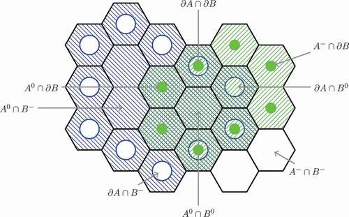
Nb. no $A^{-}\cap B^0$.

2.2. Scale

Perhaps due to its legacy evolution as an extension of computer-based maps, GIS remains largely focused on single-scale representations in a so-called “layered” representation of the world. Phenomena are discretized as thematic layers represented at a single spatial scale. Given the multi-scale properties of most natural and social processes, the single-scale view inherently limits capability for understanding cross-scale and multi-scale dynamics (Meentemeyer, 1989). As ideas are modernizing around geographic knowledge environments and the notion of digital twin systems is capable of simulating real-world complexity and dynamics, there is opportunity to make advances in multi-scale GIS (Ham & Kim, 2020; Lü et al., 2018).

DGGS offers a natural solution as a multi-scale data structure. Explicit relationships between cells in different levels of a DGGS ideally make traversing and analysis of multi-scale processes easier than with classic vector GIS representations, while the geometric and semantic flexibilities are greater than those of classic raster GIS data models. Examples of multi-scale analysis in DGGS remain limited, however, and the benefits are mostly theoretical at this stage. A simple example would be a point process with varying levels of positional uncertainty. For instance, a GPS tracking data set might have known positional uncertainties on the order of 1 m to 1000 m depending on the terrain, time of acquisition, tree canopy or building structures, etc. Traditional GIS representations of this might be to store the recorded location as spatial coordinates (i.e. point geometry) and the uncertainty as an attribute, to store the location as a region (i.e. polygon geometry) defined by the level of uncertainty, or as a range of uncertainty values bound by the limit of positional uncertainty (i.e. fuzzy representation) (Schneider, 2014). Each of these representations require special considerations for how the uncertainties might be incorporated into any analysis. A DGGS data model would employ the uncertainty-bound approach to find the best cell size approximating the location. All analysis on the data after it is imputed into the cell structure would then incorporate the spatial uncertainty, and cells at varying levels of uncertainty could be treated the same way.

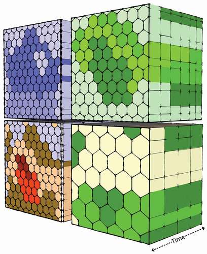
However, true multi-scale representation and analysis would make greater use of DGGS inherent multi-scale structures to model more complex phenomena. Consider, for example, a wildfire in a forest. Such a process would typically be captured by a variety of geospatial data sources such as those illustrated in Figure 5, which would need to be modelled as separate layers in traditional GIS. In DGGS, we can envisage a wildfire feature or process as a collection of cells parameterized by different data sources, with measured attributes applicable to a variety of temporal domains. Wildfire detections may be a single cell obtained from the MODIS Fire Detection System, which are captured as points representing a fire detection centroid of the 1 kilometer image cell where a fire detection occurred https://modis-fire.umd.edu/. Forest loss (i.e. due to burning) and/or fuel load (i.e. to be burned) may be captured by the change in NDVI from Landsat (e.g. 16-day intervals/30 m cells) and MODIS sensors (1-day intervals, 250 m cells). Depending on the jurisdiction, the wildfire burn extent is typically represented as vector GIS data sometimes nightly and other times shared only annually. The wind speed and direction are critical for wildfire modelling and may be obtained from point observation meteorological stations or model-derived continuous fields, which may be at a resolution of 250 m (e.g. http://globalwindatlas.info/. Terrain elevation is also critical and typically available for resolutions ranging from 5 m to 25 m for most jurisdictions. Examples such as this outlined in Figure 5 remain limited in the literature (e.g. Hojati & Robertson, 2020), as such analytical tools to model and characterize such dynamic multi-scale phenomena remain limited and need further research and development.

Figure 5. Temporal and geographical data integration for wildfire modelling. Each cube is representative of the specific theme for wildfire, and the cell size in each cube is representation of spatial resolution of the input data. The depth of each cube is the temporal dimension.

While the lack of a core feature data model for DGGS affords flexibility to model different knowledge-bases as well as multi-scale and spatially and temporally dynamic phenomena, there currently are few tools or approaches for querying and/or interrogating such representations. At the core of any DGGS data model, there are cells, sets of sells, neighbour relations, parent/child relations, and resolutions. As well, the DGGS-specific specifications such as aperture, geometry, and indexing scheme greatly affect how algorithms operate on DGGS data. How these properties are combined to facilitate multi-scale analysis is currently unclear and a key research need.

One potential solution where we expect continuous scale effects would be the estimation of mapping functions for the same variables measured at different resolutions (e.g. downscaling). Given the ability to recurse parent-child relationships, we can evaluate variable quantities (e.g. rainfall or NDVI) at intermediate resolutions. Moving further, there is potential for convolutional models that require downsampling and upsampling to incorporate DGGS data natively. A recent proposal, HexagonNet (Luo, Zhang, Su, & Xiang, 2019), exploits hexagonal DGGS geometries for convolution in a CNN context, demonstrating performance gains on aerial scene classification and 3D shape classification compared to standard geometries.

Despite the variable resolution nature of DGGS, which provides a flexible data model for representing spatial phenomena, in current DGGS implementations, there is an upper limit on resolution, which places an artificial constraint on what can be modelled. In the rHealPix DGGS, the highest resolution possible is 14 (cell area $3.7m^2$) and H3’s DGGS is 15 (cell area $<1m^2$). While DGGSs are often constructed for the global and/or national scale, there are many potential applications at more localized scales. Computational limits on higher resolution DGGS and how these might depend on system architecture remain a key area for future research. For example, sub-meter resolution cells at a global scale would likely only be feasible on a massive cloud architecture such as Amazon Web Services or Microsoft Azure. Lack of support for very high resolution cells in current DGGS implementations and software packages constrains the potential use cases to global and/or large-area mapping.

2.3. Data I/O

It is possible to consider several facets of DGGS data I/O including converting non-DGGS data into DGGS data, storage and transmitting data into a database, and visualization. Converting non-DGGS data into a DGGS model (i.e. quantization) is usually a straightforward process, which is explained in Robertson et al. (2020). A key requirement is to determine the right resolution for the target DGGS data. The uncertainty of the data can be a good estimate for the resolution of the data. Depending on the DGGS representation and selected resolution, the output data size varies and sometimes it exceeded a few terabytes for resolutions above 20, which can limit the portability of DGGS data. Storage of the data into databases can be considered as an array of cells in which for example, for a PostgreSQL, a field is limited to 1GB, so there are approximately 268 million elements in the array. Imagine that a geometry object for the border of Canada needs to be stored as a polygon in resolution 20 with aperture 3, hexagonal cell shape. It will have an approximately 129,000 cells for the border and 318 million cells for the interior. Such large arrays will reduce the performance of queries and require special consideration for algorithm development. Another method can be storing cells as long tables. Long-form tables will be able to handle larger cell numbers, but the analysis and generation of intermediate tables will create a performance bottleneck.

As noted above, the data model is different from the storage method. There are already discussions on addressing techniques to effectively store, retrieve, and transmit data sets, using efficient multi-scale data representations in DGGS models such as Mahdavi Amiri et al. (2019), Yang and Biuk-Aghai (2015), or Tripathi et al. (2016). For example, Tripathi et al. (2016) addresses methods that represent data with wavelet transforms or convert them into a wavelet-supported form, for the purposes of efficient data transmission and querying on client server platforms. DGGSs in such methods are used as a tool to efficiently manage data.

The current OGC standards for web maps and tiling schema are based on the 2D Quad TileMatrixSet methods, which is the basis for most of the current web mapping tools (OGC, 2020). There have already been DGGS tiling methods based on the rhombus (for example, Pyxis’ DGGS engine in Mahdavi Amiri et al., 2019), but the currently available tools such as map javascript libraries do not support such tiling schema. A DGGS-based VectorTile is a potential solution that can be implemented in order to visualize DGGS data. However, such tiling methods will face issues such as jittered edges due to clipping the DGGS cells by the tile boundary. Visualization of DGGS cells needs to be implemented into the current existing tools in order to provide interoperability and accessibility. In addition, pre-generation of the tiles is one of the common proposed methods (e.g. Li, Hu, Zhu, Li, & Zhang, 2017) to improve the tile-generation performance. For handling the dynamic data, it is possible to perform a value to cell join step on the client side and improve the performance of tile rendering. Since each tile in each resolution will always have a specific number of cells, there will only be a need to transfer the values of the cells for each tile.

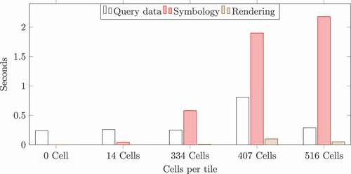
Figure 6 shows the runtime of key processing steps required for server-side rendering using current GIS visualization tools. This process is based on a standard TMS tiling service. The $x$ axis is the number of cells in each tile, and the $y$ axis is time. The first category is an empty tile, which does not have any cells in it. Rendering each tile is split into three main steps. First, query data from database. Second, based on the value of each cell, apply a proper colour to each cell and then render the set of cells. In order to apply symbology on the cells, it is required to map the data values to a symbology.Then, based on the value of the cell, a colour and related geometry are stored in an object and sent to the rendering engine to render tiles. The figure shows that while using a DGGS model and related queries, the bottleneck of the process is in the symbolizing step. However, there are several factors that need to be noticed here. First, the tile-based visualization should not be vector based and data transmission needs to be in an order of the cell location relative to the tile boundaries. Second, applying symbology can impact the overall performance considering the geographic representation of the objects. With the development of the methods such as pre-rendering tiles on the client side using predictive methods based on the end-user behaviour, more advanced GPU-based rendering and integration of the DGGS rendering methods and tilings with current existing open-source tools can solve some of the performance issues.

Figure 6. The decomposition of a sample rendering process on a server using current rendering engines (mapnik).

2.4. Benchmarking

Evaluating the performance of DGGS ultimately requires comparing them with traditional GIS models. With the introduction of new algorithms or computational tools, it is standard practice to provide a comparison with other approaches on a common task/data set in order to provide a quantitative basis for comparison. However, limited examples of performance comparison for DGGS exist in the literature such as Robertson et al. (2020).

Fundamental differences in data storage and object representation make developing comparable examples difficult. Furthermore, spatial operations on traditional data models, which are implemented in common computational tools, benefit from decades of optimization and library development, whereas newer models with less adoption require development with fewer auxiliary resources (e.g. memory allocation, geometry libraries, topological operators, etc.).

2.4.1. Spatial analysis in DGGS and vector GIS

To illustrate these interlinked issues, consider a buffer function for example. To calculate a buffer using a traditional GIS vector model, imagine that there are $n$ edges for a geometric buffer. Determining the buffer points gets completed in $O(n)$ time. For determining the intersection, we assume the worst case scenario in which each edge of a geometric buffer intersects with every other edge of the buffer, which gives $k=n(n-1)$ intersections. As a result, the highest order term will generate a complexity of $O(n2logn)$. With a general $k<n(n-1)$, the average time complexity will be $O(nlogn)$ (Bhatia, Vira, Choksi, & Venkatachalam, 2013).

In a DGGS scenario, there are several factors that need to be considered. The first item is the geometry representation whether each DGGS’s geometry is considered as an array of vertex cells or the entire array of cells comprising the geometry. In addition, the use of indexing methods can effectively change the performance of the algorithm. For example, let us say that each geometry is represented using an array of cell subset (Method 1 in Figure 1). We will need to have an ordered array of boundary cells. So the process will be a recursive algorithm, which needs to be repeated $X$ (the buffer size) times. Considering the number of boundary cells as $k$, the worst case scenario will be in $O(k^x)$. In each iteration, we need to find the neighbours of the boundary array (see Figure 7(a1)) and then find the union of them and set them as the new boundary. Following this, we attach the previous boundary to the interior array (see Figure 7(a2)). Alderson, Mahdavi-Amiri, and Samavati (2018) has proposed a similar method for offsetting spherical curves using multi-resolution DGGS grids. The cost of their method will be $O(n^2)$; however, using the multi-resolution feature of DGGS boosts the performance.

Now, consider the second method of DGGS representation (Method 2 in Figure 1). For a cubic index, $n$ points will have $O(n)$ time to compute. Per each point, we need to determine the vertex at radius $X$ in the 6 main directions around hexagonal shaped DGGS cells. The output will be $O(6n^x)$ (see Figure 7(b)). For the linear and polygon objects, the process will be the same. However, the extra step of refilling will be required to be able to represent the output geometries.

The buffer function is one of the easier examples to calculate and shows the difficulty in comparing the two different data models. Another challenge is the current status of the development of the spatial functions in databases or third-party software, which are enhanced by using internal spatial trees. Such methods can easily show better performance over DGGS-based algorithms on small machines. For example, on a machine with 64 GB of Ram, with 10 million points, a buffer in postgresql version 12 with the PostGIS extension will take an approximate 332 seconds; on the other hand, for a DGGS-based function, a buffer for the first ring will take 227 seconds, and for the second ring, it will take 692 seconds. This difference is due to two factors. First, as mentioned earlier, DGGS-based functions are usually recursive functions and as the buffer ring (in our example) increases, their performance drops. The second factor is the geometry definition. With a single resolution, as the buffer size grows, the number of cells will increase, and as a result, it will decrease performance. Another issue is the lack of optimized algorithms for DGGS-based functions. Such optimizations vary based on different indexing methods used by each DGGS, resulting in more complex optimization procedures.

Figure 7. Two different buffer algorithm methods. (a) Using the cell subset method: (a1) A recursive method. In each iteration, we first find neighbours of the border cells of the object and add them as the new border, (a2) then add the previous border to the interior cell group and at the end, remove the common cells between the new border and new interior from the new border set of cells. (b) Using the vertex cell subset method: For each cell, in the border, we first find cells in the 6 main hexagonal directions that are at the buffer distance and then remove the duplicates and store them as a subset of cells.

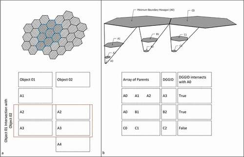
DGGS-based algorithms must consider parent-child relations and different indexing methods (such as one-dimensional space-filling curves or 2D or cubic indexes). Depending on the type of analysis, we can have the parent-child information pre-calculated in the database environment to be able to perform some of the functions; such a lookup table can be used to optimize functions, but their generation will be a time- and space-consuming process. Take the intersection function for instance, such a function can run using a table join function between two geometries (Figure 8(a)). This can be done using a one-dimensional DGGS ID. However, this only works when both input data sets are in the same DGGS representation and resolutions. Now, let us say we need to find all DGGS cells in an area. We will need to either convert the boundary box of the query area to proper DGGS cells or use the parent-child relations to access DGGS children cells Figure 8(b). For that purpose, we either need to store an array of parents for each cell to form a tree structure or have the parent-child cell relations for the entire grid in our database, or calculate parent-child relations for each cell for all the items and validate them using the parent function proposed by OGC. Both these methods need optimization methods, and some of them are not possible to perform on large data sets on a typical machine.

Figure 8. Intersection algorithm methods: (a) finding the intersection of two geometries using DGGID and the table join method and (b) finding intersecting objects with a minimum boundary hexagon and parent-child relations as auxiliary data.

The comparison of DGGS data model performance and traditional geometry object performance will require consideration of many factors, and in some cases, they are not directly comparable. In addition, in order to have a standard structure for different scenarios, it is necessary to have a standard data set. There are benchmarking for different models in traditional GIS systems such as Ray, Simion, and Demke Brown (2011). Similar efforts can be made in order to provide a test bed for the different DGGS data models. The development of community-adopted benchmark data sets will greatly facilitate method comparison and algorithm development for DGGS.

2.5. Architecture

GIS architectures have evolved from mainframe systems, to desktop computers, to web client/server systems, and to cloud and software-as-a-service (SaaS) models. While current workflows include many of these approaches and various hybrids and combinations, these systems have been developed mainly as agnostic of the underlying data models and processes, which they operate on. The benefits of SaaS, for example, are typically in terms of scale, being able to process larger geospatial data sets in less time; however, the data itself are the same representations as those on other architectures (e.g. point/line/area/raster).

DGGSs, however, represent a data model that is itself tied to an underlying architecture, primarily client/server and SaaS. Most operational DGGSs (i.e. systems not partitioning methods) exist in a cloud-native SaaS model. This necessarily limits grassroots development and experimentation with DGGS, giving rise to Digital Earth technologies more generally being part of so-called “top-down” GIS models, which can have significant impacts on the type and quality of geographic knowledge they capture (Thompson, 2016) and the potential for widespread community adoption.

Representing DGGS cells at a granular level across the entire earth requires extensive computational power. For example, given the highest available resolution available in H3, to cover entire earth surface a totals 569 trillion cells (with an area of approximately 1 sq m per cell) will be required. H3 is implemented in C and has bindings available in a variety of languages, but is interactive only through locally installed software libraries. Thus, traditional GIS tools for handling very large geospatial data sets (i.e. relational database management systems) cannot leverage these tools natively, the way it is possible via OGC data types and operators in spatial databases. This leads to more complex analytical workflows, where data and analysis are separated via network connections, and thus requires more careful planning as to where various computations are carried out. H3 can be accessed in database via PostgreSQL bindings, which requires compiling the C libraries and parameterizing to the local computational resources.

In relational database management systems, the property of data independence ensures that tables and other objects in the conceptual schema are unaffected by how data are stored on disk (i.e. physical schema). Similarly, applications that depend on data in tables and databases are independent of changes made to the conceptual schema (e.g. adding new tables, columns, or rows). Similar levels of abstraction can be applied to DGGS, where the grid definition of a DGGS is analogous to the physical schema, comprising its geometry, aperture, and orientation, perhaps even its indexing method. These properties define the DGGS and are the focus of the majority of DGGS research. Alternately, a conceptual schema for DGGS might include how cell IDs are stored, how spatial relationships are determined, and details of the feature data model, and metadata. Details on how such a conceptual schema are configured remain ad hoc and unstandardized, limiting interoperabiilty between systems at a granular level. In Robertson et al. (2020), logical data independence was achieved by developing queries and analysis in dbplyr; which separates high level analytical programming from back end database queries (Wickham, Girlich, & Ruiz, 2021). This is demonstrated through a standalone implementation of the the same application logic on SpatialLite as well as a distributed storage analytics-focused data warehouse (Hojati & Robertson, 2020).

The above discussion highlights that operationalizing DGGS, specifically the conceptual schema, data storage architectures, and retrieval/analysis tools, require further development, testing, and guidance for researchers and practitioners aiming to implement DGGS.

3. Conclusions

Discrete Global Grid Systems, which are broadly location-coding systems, are gaining traction to be a building block for the next generation of GIS. As the need for environmental information accelerates, new tools are required to meet this growing demand and harness the latest advances in data technology. In this paper, we have identified and illustrated a suite of challenges for transforming DGGS into a building block for a fully functional generic GIS. We also discussed possible paths to resolve these problems. The issues raised here are diverse in nature and encompass many core GIScience research areas. A short summary of the current challenges and some of the existing research related to them is presented in Table 2.

Table 2. A short summary of the current challenges for DGGS as a GIS and some of the existing research related to them.

Category	Research Challenge	Sample References
GIScience	Knowledge representation	2D data model: Tong et al. (2013); Robertson et al. (2020); Zhou, Chen, and Gong (2016)
		3D data model representation: Sirdeshmukh et al. (2019)
		Network topology: Dong, Chen, & Liu (2019)
	Scale	Uncertainty representation: Hojati et al. (2021, 2019); Li and Stefanakis (2020a)
		CA multi-scale analysis: Hojati and Robertson (2020)
		Convolution in a CNN context: Luo et al. (2019)
GISystems	Benchmarking	DGGS performance comparison: Robertson et al. (2020); Wang et al. (2021)
		Spatial operation comparison: Li and Stefanakis (2020b)
	Architecture	In database analytic: Robertson et al. (2020)
		Large-scale data storage: Li, McGrath, and Stefanakis (2021)
	Data I/O	Handling data sets: Mahdavi Amiri et al. (2019); Yang and Biuk-Aghai (2015); Tripathi et al. (2016)
		DGGS tiling and visualization: Mahdavi Amiri et al. (2019); Hall, Wecker, Ulmer, and Samavati (2020); Sherlock, Hasan, and Samavati (2021)

In these sections, we have discussed some of the fundamental shortcomings of representation of place/space in traditional GIS. In the context of DGGS research, we may want to revisit these fundamental concepts to go beyond a purely geometric representation of space to include more socio-cultural dimensions. Furthermore, representation of even standard GIS objects such as lines and polygons remains ad hoc in DGGS. In developing DGGS GIS, we need to consider the complexity of algorithms vs. available computational power, where computational cost can explode at higher resolutions. As such, in some cases, special SaaS architecture is required for realizing a true DGGS GIS.

Compared to well-established GIS data models, DGGS-based object interactions are poorly understood in a mathematical context. New research into topological properties would greatly benefit the development of spatial analysis methods. A multi-scale and space-time unified representation of geographic objects in DGGS is another key feature that can build towards solutions of long-standing GIS issues. However, studies examining mathematical properties and algorithm design for complex data in DGGS remain limited.

Aside from these fundamental questions, there are some key challenges at a more practical level as well. For example, there is not a clear way to benchmark DGGS-based algorithms. The mathematical efficiency of DGGS algorithms is difficult to compare traditional approaches with representation and computation. A clarity and consolidation of unified DGGS-based system architecture would also be helpful in future research. The architecture of this new GIS system in terms of database design, database bindings, visualization, and analytic workflow has to be fine-tuned and standardized to make these systems useful to non-experts and experts alike. Best practices and guidance on choosing resolution of DGGS when converting the data would facilitate more widespread uptake and exploitation of key properties of DGGS. The data fusion aspect of DGGS and its data integration for data sharing also need extensive studies to provide a clear pathway to use this framework. Recent trends towards distributed and decentralized computation are another area in which DGGS-based systems can be more useful and usable than traditional data models. The nature of the cell-based architecture lends itself to distributed computation, which may resolve some of the architecture issues noted here. As well, distributed DGGS may offer benefits in terms of digital (geo)privacy. With bottom to top data-sharing environments, it is necessary to develop tools and models to analyse, share, and integrate data at different resolutions from local to the global scale. However, considering the promise of the Digital Earth platforms to address these challenges, it can be argued that the movement is having a top to bottom development. For example, Curry (2000) argued that the Digital Earth movement is more focused on the global scale with limited local utility and that critique remains valid today. This limitation relates to knowledge representation in this platform, current accessibility of tools, and processing resources requirements. Craglia et al. (2012), in their vision for Digital Earth in 2020, consider Digital Earth as an open framework accessible to all for shaping the future of the planet. This includes small communities with limited resources, on the forefront of environmental change. However, DGGSs as an implementation of Digital Earth have not been successful in this respect due to the lack of accessible and practical tools and models. Another promise of Digital Earth is to provide a backbone for spatial data sharing (Craglia et al., 2012). However, the complexities of spatial data sharing at different levels and scales should be addressed in the Digital Earth implementations. The focus of research for DGGS as a framework for integration, management, and analysis of geographic data should be on providing more accessible procedures and applications for local communities equal to the capabilities provided at the global scale.

DGGS is in a nascent stage of development and may play an important role in the next generation of GIS. DGGS-based GIS could be the foundation of a computationally efficient, naturally multi-scale, and multi-stakeholder Digital Earth System, allowing for user-defined representations of diverse forms of geographical knowledge. However, despite the advantages that DGGS provides, there are also disadvantages that come with a new technology. Moving from current GIS data models to DGGS requires a paradigm shift. Data collection, processing, storage, analysis, and visualization systems are tied to raster and vector representations, and each of these components require new tools and optimizations. Moving data into a DGGS format requires processing time and computational power and may result in significant cartographic generalizations. The geospatial ecosystem is also uniquely structured on a large number of standards and open-source libraries, which are data model-dependent. Reconfiguring basic tools for geometry, input/output, visualization, and data quality currently requires a significant investment of time, resources, and research.

DGGS is by definition a discrete set of cells, which can result in a loss of information compared to feature data models, which may exhibit false precision and sharp boundaries. To encode information in DGGS cells, we need to specify the spatial uncertainty associated with the geographic data. While this is a benefit, in that it explicitly incorporates uncertainty, this information may be difficult to source or unknown. Also, it is unclear how spatial uncertainty embedded in DGGS analysis might impact interpretation and use of information by decision-makers who are used to seeing raster and vector data represented in geospatial products. One possible approach to address some of these issues is to treat DGGS as a backend analytic model for traditional GIS and integrate standard data models for cartographic and visualization functions. More research into decision-support dimensions of DGGS-based systems is needed. The issues raised in this paper can pave the way for future research in the DGGS domain, and we hope that it will ultimately engage the wider GIScience research community in helping to solve these challenges.

Acknowledgments

The authors thank the Global Water Futures research program for funding this work under the Developing Big Data and Decision Support Systems theme. We would also like to thank the anonymous referees for their very helpful and constructive comments.

Disclosure statement

No potential conflict of interest was reported by the author(s).

Data availability statement

Data used in this paper are available upon request from the corresponding author.

Correction Statement

This article has been republished with minor changes. These changes do not impact the academic content of the article.

Additional information

Notes on contributors

Majid Hojati

Majid Hojati is a PhD candidate in Geography and Environmental Studies at Wilfrid Laurier University. His research interest includes Geoinformatics and GIScience, web-based GIS, geographical data sharing, and geospatial big data analysis.

Colin Robertson

Dr. Colin Robertson is an Associate Professor in the Department of Geography and Environmental Studies at Wilfrid Laurier University and Director of the Cold Regions Research Centre. His research interests span the intersection of GIScience, health, and environmental change.

Steven Roberts

Dr. Steven Roberts received his PhD in Systems Design Engineering from the University of Waterloo in 2003. His doctoral work entailed the development of both the spatial data meta-model approach and prototype Evolutionary Multi-objective Optimization application using real-world GIS data sets and a Non-dominated Sorting Genetic Algorithm to solve a spatial multiobjective combinatorial optimization problem. Steve’s research interests centre on the design and development of Geographic Information Science-based tools for use in understanding landscape structures and in decision support applications for environmental land use planning. Specific fields of interest include the following: spatial data models and data structures, combinatorial optimization, genetic algorithms (Evolutionary Multi-objective Optimization), applied graph, matroid and category theory, landscape ecology, and parallel and shared memory computing.

Chiranjib Chaudhuri

Dr. Chiranji Chaudhuri loves to contribute to the research of weather modeling, hydrological modeling, environmental science, climate change analysis, and their implication on the society. He wants to become an expert in the research of climate change and its effect on the terrestrial hydrology cycle and its communication to the society. He is currently pursuing his Post-Doctoral research in Citizen Science project under the umbrella of the Global Water Citizenship program. As part of the project, he is trying to translate the modelling outputs to community information needs and vice versa using Big Data technology.

References

- Alderson, T., Mahdavi-Amiri, A., & Samavati, F. (2018). Offsetting spherical curves in vector and raster form. The Visual Computer, 34(6), 973–984.
- Appel, M., & Pebesma, E. (2019). On-demand processing of data cubes from satellite image collections with the gdalcubes library. Data, 4(3), 92.
- Barnsley, M., Møller-Jensen, L., & Barr, S. (2001). Inferring urban land use by spatial and structural pattern recognition. Remote Sensing and Urban Analysis. 115–144.
- Bhatia, S., Vira, V., Choksi, D., & Venkatachalam, P. (2013). An algorithm for generating geometric buffers for vector feature layers. Geo-spatial Information Science, 16(2), 130–138.
- Bouille, F. (1978). Structuring cartographic data and spatial processes with the hypergraph-based data structure - Structuring cartographic data and spatial processes with the hypergraph-based data structure - OICRF. Data Structures: Surficial and Multi-Dimensional, Harvard Papers on Geographic Information Systems, 5, 4–9.
- Bresenham, J. E. (1965). Algorithm for computer control of a digital plotter. IBM Systems Journal, 4(1), 25–30.
- Briggs, C., Burfurd, I., Duckham, M., Guntarik, O., Kerr, D., McMillan, M., & Saldias, D. S. M. (2020). Bridging the geospatial gap: Data about space and indigenous knowledge of place. Geography Compass, 14(11). doi:10.1111/gec3.12542
- Clementini, E., & Di Felice, P. (1996). An algebraic model for spatial objects with indeterminate boundaries. London: CRC Press.
- Craglia, M., de Bie, K., Jackson, D., Pesaresi, M., Remetey-Fülöpp, G., Wang, C., … Woodgate, P. (2012). Digital Earth 2020: Towards the vision for the next decade. International Journal of Digital Earth, 5(1), 4–21.
- Curry, M. (2000). Digital Earth, convergence, and the discursive foundations of geographic information systems. Troy, NY: Lecture given at the conference on data, for Department of Architecture, Renssler Polytechnic Institute.
- Date, C. J. (1983). An introduction to database systems (Vol. 2). Reading, Mass: Addison-Wesley Pub.
- Dong, Q., Chen, J., & Liu, T. (2019). A topographically preserved road-network tile model and optimal routing method for virtual globes. Transactions in GIS, 23(2), 294–311.
- Egenhofer, M., & Herring, J. (1990). Categorizing binary topological relations between regions, lines and points in geographic databases, the 9-intersection: Formalism and its use for natural language spatial predicates. Santa Barbara CA National Center for Geographic Information and Analysis Technical Report, 94(1), 1–28.
- Gibb, R., Cochrane, B., & Purss, M. (2021). OGC testbed-16: DGGS and DGGS API engineering report.
- Gumbula, J. N. (2005). Exploring the gupapuynga legacy: Strategies for developing the Galiwin’ku indigenous knowledge centre. Australian Academic & Research Libraries, 36(2), 23–26.
- Hall, J., Wecker, L., Ulmer, B., & Samavati, F. (2020). Disdyakis triacontahedron DGGS. ISPRS International Journal of Geo-Information, 9(5), 315.
- Ham, Y., & Kim, J. (2020). Participatory sensing and digital Twin city: Updating virtual city models for enhanced risk-informed decision-making. Journal of Management in Engineering, 36 (3), 04020005. Publisher: American Society of Civil Engineers.
- Hojati, M., Farmer, C., Feick, R., & Robertson, C. (2021). Decentralized geoprivacy: Leveraging social trust on the distributed web. International Journal of Geographical Information Science, 35(12), 2540–2566. doi: 10.1080/13658816.2021.1931236
- Hojati, M., Robertson, C., & Feick, R. (2019). Uncertainty-based representation of object-based spatial phenomena using discrete global grid systems data model. Presented at Global Water Futures Annual Science Meeting - GWF-2019, Saskatoon, SK, CA.
- Hojati, M., & Robertson, C. (2020). Integrating cellular automata and discrete global grid systems: A case study into wildfire modelling. AGILE: GIScience Series, 1, 6. Citation Key: agile-giss-1-6-2020.
- Lewis, A, Oliver, S., Lymburner, L., Evans, B., Wyborn, L., Mueller, N., Raevksi, G., Hooke, J., Woodcock, R., Sixsmith, J., Wu,W., Tan, P., Li, F., Killough, B., Minchin, S., Roberts, D.,Ayers, D., Bala, B., D., J., Dekker, A., Dhu, T., Hicks,A., Ip, A., Purss, M., Richards, C., Sagar, S., Trenham, C.,Wang, P., & Wang, L.Wei. (2017). The Australian Geoscience Data Cube — Foundations and lessons learned. Remote Sensing of Environment, 202, 276–292. doi:10.1016/j.rse.2017.03.015
- Li, L., Hu, H., Zhu, H., Li, Y., & Zhang, H. (2017). Tiled vector data model for the geographical features of symbolized maps. PLOS ONE, 12(5), 1–26.
- Li, M., McGrath, H., & Stefanakis, E. (2021). Integration of heterogeneous terrain data into discrete global grid systems. Cartography and Geographic Information Science, 48(6), 1–19.
- Li, M., & Stefanakis, E. (2020a). Geo-feature modeling uncertainties in discrete global grids: A case study of downtown Calgary, Canada. Geomatica, 74(4), 175–195.
- Li, M., & Stefanakis, E. (2020b). Geospatial operations of discrete global grid systems—a comparison with traditional GIS. Journal of Geovisualization and Spatial Analysis, 4(2), 26.
- Lü, G., Chen, M., Yuan, L., Zhou, L., Wen, Y., Mingguan, W., … Sheng, Y. (2018). Geographic scenario: A possible foundation for further development of virtual geographic environments. International Journal of Digital Earth, 11(4), 356–368. Publisher: Taylor & Francis _eprint.
- Luo, J., Zhang, W., Su, J., & Xiang, F. (2019). Hexagonal convolutional neural networks for hexagonal grids. IEEE Access, Sorrento, Italy, 7, 142738–142749.
- Mahdavi Amiri, A., Alderson, T., & Samavati, F. (2019). Geospatial data organization methods with emphasis on aperture-3 hexagonal discrete global grid systems. Cartographica: The International Journal for Geographic Information and Geovisualization, 54(1), 30–50.
- Mahdavi Amiri, Ali and Alderson, Troy, and Samavati, Faramarz. Geospatial Data Organization Methods with Emphasis on Aperture-3 Hexagonal Discrete Global Grid Systems. Cartographica: The International Journal for Geographic Information and Geovisualization, 54(1), 2019. doi:10.3138/cart.54.1.2018-0010
- Meentemeyer, V. (1989). Geographical perspectives of space, time, and scale. Landscape Ecology, 3(3), 163–173.
- Murrieta-Flores, P., Favila-vtimes New Romanã¡zquez, M., & Flores-morã¡n, A. (2019). Spatial humanities 3.0: Qualitative spatial representation and semantic triples as new means of exploration of complex indigenous spatial representations in sixteenth century early colonial Mexican maps. International Journal of Humanities and Arts Computing, 13 (1), 53–68. Publisher: Edinburgh University Press.
- OGC. (1999). OpenGIS simple features specification for OLE/COM. Revision, 1(1), 11–20.
- OGC. (2020). OGC two dimensional tile matrix set and tile set metadata. Joan Masó and Jérôme St-Louis.
- Purss, M. B. J., Peterson, P. R., Strobl, P., Dow, C., Sabeur, Z. A., Gibb, R. G., & Ben, J. (2019). Datacubes: A discrete global grid systems perspective. Cartographica: The International Journal for Geographic Information and Geovisualization, 54(1), 63–71.
- Quesnot, T., & Roche, S. (2015). Platial or locational data? Toward the characterization of social location sharing. In 2015 48th Hawaii International Conference on System Sciences, Kauai, HI, USA (pp. 1973–1982).
- Ray, S., Simion, B., & Demke Brown, Angela. (2011). Jackpine: A benchmark to evaluate spatial database performance.In 2011 IEEE 27th International Conference on Data Engineering, NW Washington, DC, United States. (pp. 1139–1150).
- Roberts, S. A., Hall, G. B., & Calamai, P. H. (2011). Evolutionary multi-objective optimization for landscape system design. Journal of Geographical Systems, 13(3), 299–326.
- Robertson, C., Chiranjib, C., Majid, H., & Roberts, S. A. (2020). An integrated environmental analytics system (IDEAS) based on a DGGS. ISPRS Journal of Photogrammetry and Remote Sensing, 162, 214–228.
- Rundstrom, R. A. (1995). GIS, indigenous peoples, and epistemological diversity. Cartography and Geographic Information Systems, 22(1), 45–57.
- Sahr, K., White, D., & Kimerling, A. J. (2003). Geodesic Discrete Global Grid Systems. Cartography and Geographic Information Science, 30(2), 121–134.
- Sahr, K. (2019). Central place indexing: Hierarchical linear indexing systems for mixed-aperture hexagonal discrete global grid systems. Cartographica: The International Journal for Geographic Information and Geovisualization, 54(1), 16–29.
- Schneider, M. (2014). Spatial Plateau Algebra for implementing fuzzy spatial objects in databases and GIS: Spatial plateau data types and operations. Applied Soft Computing, 16, 148–170.
- Sherlock, M. J., Hasan, M., & Samavati, F. F. (2021). Interactive data styling and multifocal visualization for a multigrid web-based Digital Earth. International Journal of Digital Earth, 14(3), 288–310.
- Sherlock, M. J., Tripathi, G., & Samavati, F. 2016 (December). Landsat 8 data modeled as DGGS data cubes.In AGU Fall Meeting Abstracts, San Francisco, CA (Vol. 2016, pp. IN53B–1886).
- Shuang, L., Cheng, C., Chen, B., & Meng, L. (2016). Integration and management of massive remote-sensing data based on GeoSOT subdivision model. Journal of Applied Remote Sensing, 10(3), 1–15.
- Sirdeshmukh, N., Verbree, E., Van Oosterom, P., Psomadaki, S., & Kodde, M. (2019). Utilizing a discrete global grid system for handling point clouds with varying locations, times, and levels of detail. Cartographica: The International Journal for Geographic Information and Geovisualization, 54(1), 4–15.
- Smith, B., & Mark, D. M. (2001). Geographical categories: An ontological investigation. International Journal of Geographical Information Science, 15(7), 591–612.
- Thompson, M. M. (2016). Upside-down GIS: The future of citizen science and community participation. The Cartographic Journal, 53(4), 326–334. Publisher: Taylor & Francis _eprint.
- Tim, D., Walker, S. B., & Mor, R. (2019). The state of open data: Histories and horizons. African Minds. Google-Books-ID: zKOfDwAAQBAJ.
- Tong, X. C., Ben, J., Liu, Y. Y., & Zhang, Y. S. (2013). Modeling and expression of vector data in the hexagonal discrete global grid system. In The international archives of the photogrammetry, remote sensing and spatial information sciences (Vol. XL-4-W2, pp. 15–25). Göttingen, Germany: Copernicus GmbH.
- Tripathi, G., Sherlock, M. J., Amiri, A. M., & Samavati, F. (2016). Wavelet transforms for managing landsat data sets on a geospatial client-server discrete global grid system. In AGU Fall Meeting Abstracts, San Francisco, CA (Vol. 2016, pp. IN53B–1882).
- Uber. (2020). Uber H3-js. Author. uber.github.io/h3
- Ulmer, B., Hall, J., & Samavati, F. (2020). General method for extending discrete global grid systems to three dimensions. ISPRS International Journal of Geo-Information, 9(4), 233.
- Wang, R., Ben, J., Zhou, J., & Zheng, M. (2020). Indexing mixed aperture icosahedral hexagonal discrete global grid systems. ISPRS International Journal of Geo-Information, 9(3). doi:10.3390/ijgi9090532
- Wang, Z., Zhao, X., Sun, W., Luo, F., Yalu, L., & Duan, Y. (2021). Correlation analysis and reconstruction of the geometric evaluation indicator system of the discrete global grid. ISPRS International Journal of Geo-Information, 10(3), 115.
- Wickham, H., Girlich, M., & Ruiz, E., RStudio. (2021). dbplyr: A ’dplyr’. Back End for Databases. https://github.com/tidyverse/dbplyr/
- Yang, M., & Biuk-Aghai, R. (2015). Enhanced hexagon-tiling algorithm for map-like information visualisation VINCI ’15: Proceedings of the 8th International Symposium on Visual Information Communication and Interaction , Pages 137–142.
- Yao, X., Guoqing, L., Xia, J., Ben, J., Cao, Q., Zhao, L., … Zhu, D. (2020). Enabling the big earth observation data via cloud computing and DGGS: Opportunities and challenges. Remote Sensing, 12 (1), 62. Number: 1 Publisher: Multidisciplinary Digital Publishing Institute.
- Yuan, M. (2020). Modelling semantical 1, spatial and temporal information in a GIS. In Geographic information research (pp. 334–347). London: CRC Press.
- Zhang, J., & Gong, J. (2002). Hypergraph-based object-oriented model and hypergraph theory for GIS. Geo-spatial Information Science, 5(1), 37.
- Zhou, M., Chen, J., & Gong, J. (2016). A virtual globe-based vector data model: Quaternary quadrangle vector tile model. International Journal of Digital Earth, 9(3), 230–251.