EASE-DGGS: a hybrid discrete global grid system for Earth sciences

ABSTRACT

Although we live in an era of unprecedented quantities and access to data, deriving actionable information from raw data is a hard problem. Earth observation systems (EOS) have experienced rapid growth and uptake in recent decades, and the rate at which we obtain remotely sensed images is increasing. While significant effort and attention has been devoted to designing systems that deliver analytics ready imagery faster, less attention has been devoted to developing analytical frameworks that enable EOS to be seamlessly integrated with other data for quantitative analysis. Discrete global grid systems (DGGS) have been proposed as one potential solution that addresses the challenge of geospatial data integration and interoperability. Here, we propose the systematic extension of EASE-Grid in order to provide DGGS-like characteristics for EOS data sets. We describe the extensions as well as present implementation as an application programming interface (API), which forms part of the University of Minnesota’s GEMS (Genetic x Environment x Management x Socioeconomic) Informatics Center’s API portfolio.

KEYWORDS:

• Discrete global grid systems
• DGGS
• EASE Grid
• coordinate reference systems

1. Introduction

We live in an unprecedented era, where quantitative descriptors are collected for nearly every facet of human development and natural phenomena we collectively deem important (Miller & Goodchild, 2015; Rosling, Rosling, & Ronnlund, 2020). In the Earth sciences alone, individual data archives exceed the petabyte scale; in 2015 alone NASA’s Earth Observing System (EOS) Data and Information System distributed more than 9,400 distinct data products to 2.6 million distinct users (Lynnes, Baynes, & McInerney, 2016). While EOS data have always been big data, both the rate at which we are accumulating it and the variety of data we gather are rapidly increasing (Open Geospatial Consortium, 2017a). Accompanying the rapid expansion of Earth observing systems, advances in portable electronics have also resulted in exceptional growth in global sensor networks (Purss et al., 2017). This proliferation of sensors has shifted scientific computing away from a centralized paradigm to one where analytical processes are increasingly distributed across systems connected via the Internet.

In isolation, individual sets of descriptors, whether they are from Earth observation platforms or sensor networks, have limited utility or intrinsic value. It is mainly through integration and combination with additional descriptors that patterns emerge, relationships are quantified, and information can be derived from raw data. Information, in turn, fuels insight and scientific understanding, key requirements for evidenced-based decision-making. Since its inception as a quantitative discipline, geographic information science has been driven by a desire to apply quantitative methods to Earth observation information to improve resource management decision-making (Goodchild, 2018; Peterson, 2017). Seemingly simple questions such as: ’how much suitable land is available for agricultural uses that is not already being used for other purposes?’ motivated the development of early geographic information systems (GIS).

The integration of disparate geospatial data types is traditionally a hard problem. The difficulties in combining geospatial data have historical roots in technological limitations of early computers during the shift from predominantly qualitative uses of cartographic maps to the emergence of quantitative, geospatial analysis (Goodchild, 2018). Early geographic information systems were predominantly centered on vector data types (points, lines, polygon) (Goodchild, 2018), though subsequent developments gave rise to systems that dealt primarily with gridded data types, like rasters/imagery (Peterson, 2017). The partitioning of the geospatial world into vector-based and raster based solutions persists today, making the original aim of integration and inter-operation of geospatial data for resource management decisions possible, but it requires considerable time and the expertise of highly trained professionals (Goodchild, 2018).

The rise of the Internet and its capacity for rapid global data transfer has simultaneously driven expectations and desires to accelerate information generation processes to support decision-making in near real-time. The historical legacies of traditional GIS software, tools, and data formats constrain the capacity to increase the rate at which information are gleaned using disparate geospatial data sets. Technological innovations are needed to overcome traditional limitations (Goodchild, 2018). The technology of discrete global grid systems (DGGS) has been proposed as one means of overcoming those limitations, thereby enabling potentially accelerated information discovery processes using geospatial data (Open Geospatial Consortium, 2017c).

Within the Earth observation community, the need to increase the rate of information production has resulted in several domain-specific solutions. Innovations designed to reduce data processing overhead have included: shifting away from minimally processed data towards the production of data that are analysis ready (Dhu et al., 2017; Dwyer et al., 2018; Potapov et al., 2020) and the creation of image processing frameworks, such as data cubes, which allow for increased integration of Earth observation data from different sensor types and resolutions (Lewis et al., 2017). These systems are predominantly geared towards data processing, and not towards facilitating data integration, creating interoperable data types or accelerating information generation from disparate sources.

DGGS are a technology designed specifically for data integration and information retrieval. They have been proposed as a useful technology for solving the issues with data integration, thereby accelerating the ’geospatial intelligence cycle’ (Consortium, Open Geospatial, 2017c). The aim of this paper is to present and describe a hybrid DGGS built upon the Equal-Area Scalable Earth Grid (EASE-Grid 2.0, hereafter, EASE-Grid) framework of Brodzik, Billingsley, Haran, Raup, and Savoie (2012, 2014). We refer to the proposed system as EASE-DGGS. To demonstrate the need and utility for EASE-DGGS, we describe key aspects of DGGS, before reviewing current DGGS solutions. The review highlights the limitations of current DGGS offerings, notably their limitations regarding common Earth observation systems. We propose a solution that leverages the enhanced EASE-Grid solution described by Brodzik et al. (2012, 2014). We discuss the foundational components of EASE-Grid, before discussing our solution for systematizing a nested hierarchy of grids, thereby creating a DGGS framework from EASE-Grid.

2. Discrete global grid systems

Despite the fact that early DGGS efforts date back to the mid-1980s with the work of Tobler and Chen (1985) there have been few widely available DGGS options until recently. In recent years, there appears to have been a flurry of activity, with new systems proposed that include: H3, the hexagonal grid system that underpins Uber Technology’s market-based ride sharing application (2018); and rHEALPix, a quadrilateral DGGS proposed by Gibb (2016). Open-source software repositories exist for both H3 (2018) and rHEALPix (2021). Application of the rHEALPix DGGS to Australia and New Zealand were presented by (Purss et al. (2013), use in Canada examined by Bowater and Stefanakis (2018), and its application to a gazetteer can be found in Adams (2017). Readers interested in the origins of DGGS and the limitation of traditional GIS systems are directed to Goodchild (2018) and Peterson (2017). While comprehensive review of the DGGS literature and associated design criteria are beyond the scope of this paper, a review of some salient technical details of DGGS their design characteristics is presented in the Supplementary Materials. For convenience, a brief overview of the key aspects of DGGS and some of their limitations are discussed below.

2.1. Key aspects of discrete global grid systems

In essence, DGGS are a technology that have been proposed to overcome limitations of traditional spatial analysis (Goodchild, 2018; Peterson, 2017). A DGGS provides a way of referencing geospatial information that embraces the realities and inherent uncertainties associated with geolocating observations (Goodchild, 2018; International Standards Organization, 2021; Purss et al., 2015) and they seek to accelerate and enhance the retrieval of spatial information from underlying databases (International Standards Organization, 2021). The aim of a DGGS is to effectively engineer away the more time consuming, arduous, and subjective analytical decisions that often fall under the purview of ’data preprocessing’ in the remote sensing and GIS literature.

At its core, a DGGS is a spatial reference system for the surface of the Earth (International Standards Organization, 2021). With traditional coordinate reference systems, spatial locations on the Earth’s surface as characterized using tuples of coordinates, such as: longitude, latitude or eastings, northings. In contrast, DGGS use aerial units, or grid cells, to describe locations on the surface. In this sense, a DGGS is similar to the traditional raster data model, which also uses areal units (pixels) to store geospatial information. Whereas traditional rasters comprise rectangular cells, the grid cells of a DGGS are not similarly constrained: common regular polygons used in DGGS include squares, triangles, and hexagons (Mahdavi Amiri, Alderson, & Samavati, 2019; Peterson, 2017).

Because the grid cell is the basic spatial unit within a DGGS, the grid identifier (ID) becomes the way of referencing spatial locations. There are at least three primary methods for assigning identifiers (Alderson, 2020): hierarchy-based indexes; indices based on space-filling curves; or axes-based indexing (see Supplementary Materials). Irrespective of their underlying derivation, the grid ID provides the spatial reference, with each grid ID representing a unique, and discrete portion of of the Earth’s surface. Because DGGS are intended to simplify and facilitate spatial analysis, it is desirable that DGGS grid cells should represent equivalent areas of the Earth’s surface (Tobler & Chen, 1985). That is, DGGS grid cells should be equal in area; many resource management, economic, or agricultural analyses involve spatial inter comparison comparison between derived statics, such as densities or rates, in order to arrive at a relevant decision.

Finally, DGGS have one additional key characteristic: that of hierarchical refinement (Supplementary Materials). A traditional raster has a single, fixed resolution. In contrast, a DGGS comprises multiple grids, arranged in a hierarchical fashion, with each level in the hierarchy representing progressively finer, and finer spatial resolutions (Goodchild, 2018; Peterson, 2017; Tobler & Chen, 1985). While a spatial analyst can always resample a traditional raster to some arbitrary coarser or finer spatial resolution, the resolutions of a DGGS are essentially fixed. They are an intrinsic property of the grid system, and defined in advance, when the system is constructed.

2.2. Limitations of DGGS for integrating E0S data

A comparative review of several state-of-the-art DGGS was recently presented by Bondaruk, Roberts, and Robertson (2020). Their review assesses four DGGS for compliance with the DGGS standards proposed by the Open Geospatial Consortium (2017c). An updated summary of their assessment is presented in the Supplementary Materials; that summary also includes an assessment the of rHEALPix DGGS proposed by Gibb (2016). Rather than providing a comprehensive critique of DGGS, the main aim here is to draw attention to potential limits of DGGS for integrating EOS data. These limits form the basis the proposed EASE-DGGS.

EOS data are an increasingly valuable and important source of spatial information. In spite of this, there is a challenge when trying to determine a DGGS that is suitable for use with EOS data. One challenge relates to finding a DGGS with cell resolutions that correspond with the native pixel resolution of EOS datasets. Table 1 presents a range of pixel sizes associated with EOS data that either have a history of use in the Earth sciences (e.g. Landsat, MODIS) or newer systems that build upon the legacy of established sensors (e.g. Sentinel-2, VIIRS). Also included in that list are high-resolution commercial sensors that have been employed in Earth sciences (WorldView) as well as a commercial constellation of high-spatial sensors (Planet) that in concert effectively sample the Earth’s surface with unparalleled temporal frequency. Table 2 presents the grid cell resolutions for both H3 and resolutions for two different refinement ratios for rHEALPix. When considering the range of spatial resolutions of EOS systems (Table 1), it is clear that there is no obvious, direct correspondence between the resolutions of EOS systems (Table 1) and those available in either H3 or rHEALPix (Table 2).

Table 1. Example of common Earth observation systems and their respective pixel sizes.

EO System	On-ground resolutions (m)
WorldView-3	0.31/1.24/3.70
Planet	0.50
SPOT-7	1.5/6
Sentinel-2	10/20/60
Landsat-8	15/30/100
MODIS	250/500/1000
VIIRS	375/750

Table 2. Comparison of cell sizes between H3 and rHEALPix at various refinement ratios. For this comparison, H3 cells are treated as a circle with an equivalent diameter.

DGGS	H3	rHEALPix	rHEALPix	rHEALPix
Ref. Ratio	7	4	9	14
Level	Equiv. diameter (m)	Cell Width (m)	Cell Width (m)	Cell Width (m)
0	2,326,362.90	10,013,169.15	10,013,169.15	10,013,169.15
1	879,282.53	5,006,584.58	3,337,723.05	2,503,292.29
2	332,337.56	2,503,292.29	1,112,574.35	625,823.07
3	125,611.79	1,251,646.14	370,858.12	156,455.77
4	47,476.79	625,823.07	123,619.37	39,113.94
5	17,944.54	312,911.54	41,206.46	9778.49
6	6782.40	156,455.77	13,735.49	2444.62
7	2563.51	78,227.88	4578.50	611.16
8	968.91	39,113.94	1526.17	152.79
9	366.22	19,556.97	508.72	38.20
10	138.42	9778.49	169.57	9.55
11	52.32	4889.24	56.52	2.39
12	19.77	2444.62	18.84	0.60
13	7.48	1222.31	6.28	0.15
14	2.83	611.16	2.09	0.04
15	1.07	305.58	0.70	0.01

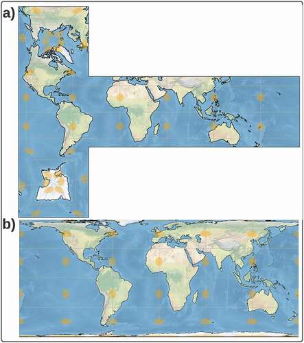
Another challenge with most DGGS is their relative lack of support within existing geospatial libraries and software. For example, very few of the existing systems appear to have much support for the common formats used to convey spatial reference information: EPSG codes, Well-known-text, or proj-4 codes. rHEALPix Gibb (2016) is an exception, as it does have a proj-4 entry. The Snyder icosahedral projection (Snyder, 1992), which underpins several DGGS (e.g. Barnes and Sahr (2018), Technologies, Uber (2018), and Ltd., Riskaware (2017)), also has a proj-4 entry, though the specific DGGS implementations do not. Finally, nearly all of the currently available DGGS are limited in their capacity to simultaneously represent the entire surface of the Earth. Although the 3D basis of geodesic reference systems generally results in overall less distortion of the Earth’s surface (Purss et al., 2017; Sahr, 2003), the underlying choice of a platonic solid results in discontinuities and distortions of geographic features along the edges of the platonic solid, particularly when the entire Earth surface is represented simultaneously (Snyder, 1992). An example of these types of discontinuities is evident in Figure 1(a). The choice of orientation of the figure results in land mass of North America remaining intact, while the continents of Europe and Asia are divided across two panels. Although alternative representations are possible, for example those that emphasize more of Asia or Europe, there is no representation that results in the Eurasian landmass remaining intact. Furthermore, geographic discontinuities will be more pronounced on DGGS where a higher order platonic solid is use for the underlying datum. Ultimately, the choice of whether or not to trade off discontinuities in geographic features for potential reductions in overall surface distortion likely depends on the aims of the analyst and the uses for which a proposed DGGS is envisioned. To a polar scientist, the distortions evident in both Figure 1(a,b) are likely unacceptable as would be a DGGS based on them. To an agronomist and agricultural economist interested in understanding and characterizing the global distribution of crop production in a changing climate, being able to visualize and compare different regions at a glance (1 b) may ultimately be worth the trade off in distortion at the extreme poleward extents of the map.

Figure 1. Comparison of the discontinuities and distortions of two equal area representations of the Earth’s surface: a) representation using the rHEALPix hexadron datum; and b) projected representation using EASE Grid version 2. Note that the Orange ellipses are Tissot’s indicatrices, which indicate the amount and direction of surface distortion at various locations.

3. Systematic extension to EASE-Grid 2.0

One of the motivations for developing the work described below is to facilitate the data integration process for agroinformatic analyses. The Genomics x Environment x Management x Socioeconomic (GEMS) is an initiative at the University of Minnesota that seeks to accelerate agricultural innovation and research by bringing the data revolution to agriculture. GEMS is an international agroinformatics initiative jointly led by the College of Food, Agricultural and Natural Resources Sciences (CFANS) and the Minnesota Supercomputing Institute (MSI) at the University of Minnesota. GEMS seeks to turn agricultural data into actionable information by making data interoperable across knowledge domains, and foster data sharing and innovation across public and private interests.

When considering the need for solutions that accelerate the rate at which information is derived from geospatial data, a primary source of much of that data are and will increasingly be from Earth observation systems. Considering the limitations of current DGGS outlined above, there is a need for a DGGS system that simultaneously addresses both needs and limitations. We have created such a system, and in this section we describe it and key functional aspects and components. Because the system is built upon the revised EASE-Grid projected coordinate reference systems described by Brodzik et al. (2012) and Brodzik et al. (2014) we start by presenting key aspects of EASE-Grid version 2, before moving on to describe the systematization and characteristics of what we call EASE-DGGS and its implementation as an application programming interface (API) within the GEMS Informatics Center’s API portfolio.

3.1. Advantages of EASE-Grid

The original intent of the Equal-Area Scalable Earth Grid (EASE-Grid) was for storage and retrieval of passive microwave observations obtained by the Special Sensor Microwave Imager (SSM/I) on-board the NOAA/NASA Pathfinder satellite (Brodzik & Knowles, 2002). The intent of EASE-Grid was for a coordinate reference system that served as a ’fixed geographic look-up table’ but also a system that faithfully represented the underlying resolution and fidelity of the original passive microwave observations of the Earth’s surface. The original EASE-Grid specification described 25 × 25 km grid lattices for Lambert’s azimuthal projections of both northern and southern hemispheres, as well as an equal area cylindrical projection for the entire globe. A convenient side effect of the equal-area design choices for EASE-Grid was the simplicity of areal statistical calculations, leading to a secondary meaning for EASE; meaning the grid was ’easy to use.’

The popularity and success of the original EASE-Grid prompted Brodzik et al. (2012) and Brodzik et al. (2014) to eventually both refine and extend the original system. One improvement was to reference the version 2 grids to the WGS-84 datum rather than to the spherical datum of the original. This change in datum was intended to increase the likelihood that common geospatial libraries and packages would be able to better accommodate the new grid, thus reducing the possibilities for introducing errors into analyses. Another improvement adopted into version 2 of EASE-Grid was the choice to nest child cells. Whereas the original EASE-Grid definitions resulted in imperfect containment of child cells by their parents when refined, the current specification for EASE-Grid (version 2) results in perfect containment of children by parents.

Clarke (2000) noted that broad uptake and citation in the literature are indicators of authority and an additional criterion for discrete global grid systems. The ’easy-to-use’ moniker of the original EASE-Grid remains, as it has been adopted by a number of different data providers. Amongst the data sets and providers that have reported adopting the updated version of EASE-Grid include the global SMOS soil moisture and brightness temperature (Al Bitar et al., 2017), MEaSUREs enhanced brightness temperatures (Brodzik, Long, Hardman, Paget, & Armstrong, 2016), MEaSUREs Northern Hemishpere weekly snow-cover and sea-ice extent (Brodzik & Armstrong, 2013), SMAP rSIR version 1 (Brodzik, Long, & Hardman, 2019) and 2 (Brodzik, Long, & Hardman, 2021), SMAP 9 km (Entekhabi, Das, Njoku, Johnson, & Shi, 2016), SMAP 3 km (Kim et al., 2016), SMAP landscape freeze-thaw (Kim, Kimball, Glassy, & Du, 2017a), MEaSUREs freeze-thaw (Kim, Kimball, & McDonald, 2017b), Arctic sea-surface salinity (Martínez, Gabarró, & Turiel, 2019), MEaSUREs Greenland surface melt (Mote, 2014), and Northern Hemisphere snow cover extent (Robinson & Estilow, 2012).

3.2. EASE-Grid extension

EASE-Grid version 2 defines grids at several different resolutions. These resolutions can be categorized as representing either refinements of base 25 × 25 km cells (e.g. 12.5 × 12.5 km, 6.25 × 6.25 km, and 3.125 × 3.125 km) or refinements of base 36 × 36 km cells (9 x 9 km, 3 × 3 km, and 1 × 1 km). For the systematization described here, we chose the 36 km as the basis for EASE-DGGS and we further propose additional refinement down to 1 × 1 m. Table 3 contains the full specification of cell refinements and with associated refinement ratios. Note that whereas other DGGS tend to opt for a single fixed refinement ratio throughout their hierarchy, we have opted for mixed refinement ratios, to allow for improved correspondence with common sources of Earth observation data (Table 1). To maintain perfectly square grid cells, EASE-DGGS described herein is further constrained to locations between longitude of −180.0 to 180.0 and latitudes of 85.045 to −85.045 (Table 4).

Table 3. Refinement ratio for each level of EASE-DGGS and corresponding cell resolution. Refinement ratio is currently not defined below Level 6.

Level	Ref. Ratio	Num. Cells	Cell dimensions [meters]
0	16	391,384	36,032.22084 × 36,032.22084
1	9	1,565,536	9008.05521 × 9008.05521
2	9	4,696,608	3002.68507 × 3002.68507
3	100	14,089,824	1000.89502 × 1000.89502
4	100	140,898,240	100.08950 × 100.08950
5	100	1,408,982,400	10.00895 × 10.00895
6	N.D.	14,089,824,000	1.000895 × 1.000895

Table 4. Longitude, latitude, and EASE-Grid coordinates (x, y) for the upper left and lower right of the EASE-DGGS.

Grid locations	Longitude	Latitude	EASE X [m]	EASE Y [m]
Upper-left	−180.0	85.04456640	−17,367,530.445161372	7,314,540.830638504
Lower-right	180.0	−85.04456640	17,367,530.445161372	−7,314,540.830638504

For indexing the grid cells, we employ a hierarchical approach (Figure 2)

Figure 2. Hierarchical schema and decomposition of the Grid ID naming convention.

that also incorporates an axis-based solution (Figure 3)

Figure 3. Representation of the address-indexing scheme underpinning EASE-DGGS. Note that all coordinate pairs are in y, x (row, column) order.

. Because children are perfectly nested within parent cells (Brodzik et al., 2012), we start by referencing cells by rows, starting from the upper left corner of the grid (Figure 3). Thus at the highest level of the hierarchy (Level 0) cells are referenced using both their three digit row number (000–405) followed by their column number (000–963). With further refinement, the base index is appended, following the row-major format. For Level 1, the Level 0 parent is appended with the row, column index of the refined child cell (Figure 2).

Clarke (2000) also indicated that grid systems that are intuitive and easier to use are preferable to those that are not. In line with this thinking, we adopt a dotted decimal notation: levels are separated using ’.Figure 3’. In addition, the hierarchical level of the cell is also indicated using an L, with an integer corresponding to the level within hierarchy (Level 0: L0, Level 1: L1, etc – 2). This dotted decimal notation is similar to the familiar Internet Protocol Addressing (v4). It makes identifying parent cells, and navigating up the child-parent hierarchy a straightforward process. The indexing scheme also has the added benefit that indexes also represent the location of the refined cell within each parent. That is, starting from the upper left corner of parent, the cell identifier represents both the index and location of the child within its parent cell. Although the hierarchical dotted decimal format is selected for the purpose of ease of use and human readability, it is noted that it is possible to represent the entire scheme using 64-bit integers (Table 5).

Table 5. The address-indexing scheme is compatible with a 64-bit address space representation.

Bit Range	Type	Description
0–6	Bit flag	Indicates hierarchy level.
7–15	Integer	Indicates Level 0 row.
16–25	Integer	Indicates Level 0 column.
26–29	Integer	Indicates Level 1 pixel location in Level 0 cell.
30–33	Integer	Indicates Level 2 pixel location in Level 1 cell.
34–37	Integer	Indicates Level 3 pixel location in Level 2 cell.
38–45	Integer	Indicates Level 4 pixel location in Level 3 cell.
46–52	Integer	Indicates Level 5 pixel location in Level 4 cell.
53–59	Integer	Indicates Level 6 pixel location in Level 5 cell.
60–63	–	Unused.

3.3. Implementing an API for the GEMS Platform

We implemented the EASE-DGGS library in the python programming language and have developed a publicly accessible API. Documentation for the API functionality and schema is available through the URL: https://gems.umn.edu/exchange/grid with supported methods accessible through this URL. It contains functions for converting from geographic coordinates to EASE-DGGS grid IDs, and for converting from grid IDs to geographic coordinates (Table 6). There are also functions for enumerating the children of parent cells by level, and the reverse. The library also contains functions for identifying all grid IDs that are contained within geographic polygons (e.g. polygons as WKT). Aggregation functions that allow for summarizing data at coarser resolution (e.g. counts, means, modes, medians) have also been implemented within the API.

Table 6. Initial functions supported by GEMS Grid API.

Function Name	Description
points_to_grid	Map points (and optional values) to GEMS Grid cells at provided resolution.
poly_to_grid	Given a GeoJSON polygon and a specified grid resolution level, return the corresponding GEMS grid cell IDs.
grids_to_geom	Given a list of GEMS grid cell IDs, return a list of lon/lat values corresponding to the grid cell centroids and a polygon. Output points provided in GeoJSON.
get_grid_parents	Given a list of GEMS grid cell IDs, return a list of the parents of those grid IDs.
get_grid_children	Given a list of GEMS grid cell IDs, return a nested list of the children of each input grid ID
aggregate	Given GEMS grid cell IDs with a value associated with each Grid ID, return corresponding GEMS grid cell IDs with aggregated values at a specified grid resolution level coarser than that provided.

4. Discussion

In this manuscript, we have proposed the systematic extension of EASE-Grid in order to give it the key characteristic of a DGGS. These extensions are intended to overcome limitations associated with existing DGGS. The advantages of the proposed systems include improved correspondence with EOS observations, broad compatibility with existing geospatial software and underlying libraries, as well as good support for global visualizations and analysis. This section discusses these advantages, in addition to outlining and addressing the broader challenges associated with accelerating the rate of information and knowledge generation from EOS data.

The improved correspondence between EOS observations and the resolutions supported by EASE-DGGS are one advantage of the proposed extension. EOS observations are an important data source for resource management and agricultural applications, and being able to combine data obtained at different resolutions is a common, pre-processing step in image analysis. Decisions regarding image re-sampling have traditionally relied upon the judgment and experience of the image analysts, and it was the analysts themselves that were responsible for ensuring that data sets were spatially aligned, with common dimensions. Systematizing and specifying the hierarchy of supported resolutions and defining the rules for navigating the hierarchy in advance means that the analyst need only define the spatial extent for a given analysis, and select a resolution for analysis. This ensures that data are spatially aligned, and have shared image dimensions (e.g. identical numbers of rows, columns).

Another advantage of the proposed system is that EASE-Grid, the spatial reference system underpinning EASE-DGGS, is readily compatible with widely used software and libraries. For example, EASE-Grid has an entry in the European Petroleum Survey Group (EPSG) registry, which is commonly supported format that allows for seemless integration with a wide variety of both commercial geospatial software and open-source libraries. In contrast, the spatial referencing systems that underpin existing DGGS currently either require specific libraries in particular programming languages, such as dggridR (Barnes & Sahr, 2018) or where they have been made available in multiple languages (e.g. H3 of Technologies, Uber (2018)), their use still requires considerable technical and programmatic ability.

The final advantage of the proposed system pertains to visualisation of global data sets. Because most of the existing DGGS are constructed using geodesic reference systems (e.g. using platonic solids) there are challenges when using them displaying the entirety of the Earth’s surface (Snyder, 1992). This limitation is often dismissed as being of secondary importance, as it only relates to visualization, (e.g. Goodchild, 2018). The view that visualization is somehow secondary in importance to computation or analysis is not new; similar debate regarding the ’proper’ or appropriate role of visualization in statistics was addressed in the 1970s by Anscombe (1973). Similarly, rather than suggesting visualizations only play a secondary role in geospatial analysis, we suggest instead that visualization itself is integral to the analytical process. Often it is the context of characterising ’what’ alongside the ’where’ that testable hypothesis of ’how’ and ’why’ of spatial phenomenon are formed (Yuan, 2020). Because spatial analyses have only tended to addressed questions of local or regional relevance (Goodchild, 2018), this lack of good, global visualization capacity has likely contributed to the perception that geospatial visualization is of secondary importance. Because our primary interest is to characterize, understand, and improve global agricultural practices in the context of climate change, we suggest that visualization itself is an integral part of geospatial analysis in this context.

The importance of analytical context cannot be understated, nor should it be summarily dismissed. It is important to recognize that DGGS are at heart a form of spatial reference system designed to address the limitations associated with traditional geospatial analysis (Open Geospatial Consortium, 2017c; International Standards Organization, 2021). In some senses, DGGS have similarities with traditional map projections and coordinate reference systems that they seek to replace. It is worth noting that, to date, no one single ’ideal’ map projection has ever been identified unless the design requirements have been arbitrarily restricted (Snyder, 1997). Similarly, given the trade-offs inherent in DGGS design characteristics, it seems unlikely that consensus will emerge on an ’ideal’ reference system. Hence an ’optimal’ DGGS will likely remain elusive.

In addition to the advantages outlined above, as noted previously, EASE-Grid itself has already been adopted as the spatial reference system by several different EOS data providers. This uptake is important; part of the OGC’s rationale for DGGS is the recognition that traditional data archives need to adopt new data models and formats (Open Geospatial Consortium, 2017b). EASE-Grid addresses many of the limitations of other coordinate reference systems (e.g. Mercator, plate carrée) identified by the OGC as motivating the development DGGS (International Standards Organization, 2021). According to Clarke (2000), the adoption of EASE-Grid by the remote sensing community can be construed as providing additional justification and legitimacy to the approach presented herein. It should also be noted that the approach outlined herein shares similarities with the DGGS solution posited by Tobler and Chen (1985).

As noted in the Introduction, the current volume of public EOS data is already substantial. The rate of data acquisitions is only accelerating, as commercial companies now image the entire Earth’s surface with both high spatial and temporal frequency. While the aim of DGGS is to facilitate the creation of information and knowledge by engineering away limitations of traditional GIS systems thereby removing analytical barriers (Open Geospatial Consortium, 2017b). it is important to acknowledge that a single ’ideal’ or ’optimal’ DGGS reference system may ultimately prove unobtainable. Irrespective of whether or not an ’optimal’ system could be agreed upon, the amount of time, energy, and effort required to reprocess entire image repositories would likely prove to be a substantial barrier for adoption. This highlights the need to bring the remote sensing community, geospatial professionals, and big data engineers together to identify ways in which existing technologies and solutions can be leveraged to address these issues.

5. Conclusion

We have presented a systematic extension of EASE-Grid 2.0, which was originally described by Brodzik and others (Brodzik et al., 2012). We refer to this systematic extension as EASE-DGGS. This framework leverages the base 36 × 36 km spatial resolution and provides for grid cell indexing to 1 × 1 m resolution. This proposed framework overcomes the limitations of existing DGGS frameworks. It provides better correspondence between the DGGS and the native resolution of many common Earth observation platforms. Additionally, it also overcomes specifics limitations of H3, notably the lack of parent–child containment and the associated lack of statistical inversion between levels.

It is noted that further refinement of the system is possible. For example, a Level 7 refinement using refinement ratio 4 would result in cells that approach the resolution of the Planet constellation of satellites and sensors (0.5 x 0.5 m). Although EASE-DGGS does more closely represent the native resolutions of Earth observation systems (Table 1) it does so at the expense of an increase in data storage volumes. Representing a single 30 m Landsat pixel, for example, requires using multiple Level 5 pixels. This represents an increase in storage volume by a factor of 9 times. Similarly, accommodating 500 m MODIS pixels at approximately their native resolution would increase storage requirement by 25 times.

In spite of this limitation, we propose that the systematic extension of EASE-Grid into a DGGS offers a potential advantage over existing DGGS particularly for integrating existing EOS data streams. Given the strong adoption of EASE-Grid version 2 within existing Earth science data streams, EASE-DGGS can provide a framework that enables interoperability, thus offering the potential for accelerated information generation from those Earth observation data streams.

Disclosure statement

No potential conflict of interest was reported by the author(s).

Data availability statement

There are no data associated with this manuscript.

Supplementary Material

Supplemental data for this article can be accessed online at https://doi.org/10.1080/20964471.2021.2017539.

Additional information

Funding

Funding for Jeffery A. Thompson’s and Kevin Silverstein’s time is funded by the Minnesota Supercomputing Institutue under the partnership between the University of Minnesota and the state of Minnesota as part of Minnesota’s Discovery, Research, and InnoVation Economy (MnDRIVE). Mason Hurley 's contribution in implementing the DGGS framework are provided by the College of Food, Agricultural and Natural Resource Sciences (CFANS) of the University of Minnesota. Nathan Carlson’s contributions to the API are funded by the Minnesota Supercomputing Institute.

Notes on contributors

Jeffery A. Thompson

Jeffery A. Thompson is a High-Performance Computing Geospatial Scientist within the Minnesota Supercomputing Institute (MSI) at the University of Minnesota. He obtained a masters degree in Geographic Information Sciences and a second masters in Resource Science from the University of New England, Australia. He also holds a PhD in Geography from the University of New South Wales, Australia. He has more than a fifteen year of experience applying remote sensing and geospatial data within Earth and environmental sciences. His primary research interest is in applying remotely sensed image time-series to phenological studies, and he is particularly interested in im- proving our understanding of the interactions between vegetation and eco-hydrological dynamics. Having worked on projects in agriculture, mining, resource management and environmental issues, his geospatial experience is wide ranging.

Mary J. Brodzik

Mary J. Brodzik received the B.A. degree summa cum laude in mathematics from Fordham University, Bronx, NY, USA, in 1987. She is a Senior Associate Scientist at the National Snow & Ice Data Center (NSIDC), Cooperative Institute for Research in Environmental Sciences (CIRES), University of Colorado Boulder, Boulder, Co, USA. Since coming to NSIDC in 1993, she has implemented software systems to de- sign, produce, and analyze snow and ice data products from satellite-based visible and passive microwave imagery. She has contributed to the NSIDC data management and software development teams for the NASA Cold Lands Processes Experiment and Operation IceBridge. As a Principal Investigator of the NASA Making Earth Science Data Records for Use in Research Environments Calibrated Enhanced-Resolution Brightness Temperature Project, she managed the operational production of a 40+ year EASE- Grid 2.0 Earth Science Data Record of satellite passive microwave data, and related enhanced-resolution SMAP images. She is using MODIS data products to derive the first systematically derived global map of the world’s glaciers. For the U.S. Agency for International Development, she developed snow and glacier ice melt models to better understand the contribution of glacier ice melt to major rivers with headwaters in High Asia. Prior to her work at NSIDC, she worked in software development, validation and verification on Defense Department satellite command and control and satellite track- ing systems. Her research interests include optical and passive microwave sensing of snow, remote sensing data gridding schemes, and effective ways to visualize science data.

Kevin A. T. Silverstein

Kevin Silverstein is Scientific Lead for the Research Informatics Solutions (RIS) group at the Minnesota Supercomputing Institute (MSI) and Operations Manager of the GEMS Agroinformatics Initiative. He has spent decades performing large-scale bioinformatics analyses involving cutting-edge high-throughput data from bacteria, fungi, plants, mammals and complex communities. He has performed detailed investigations of plant-microbe systems in continued research since 2001. Additionally, in 2010–2012, he led an effort to identify mutations in clinical patients with Fairview Hospital which has been expanded in partnership with MSI and continues to be used today. The knowledge gained from handling protected patient data has been brought over to the GEMS platform to protect farmer and corporate data.

Mason A. Hurley

Mason Hurley is a Data Engineer within the GEMS Agroinformatics Center (GEMS). He graduated from the University of Minnesota with an M.S. in Applied Economics. He spent several years as a Data Scientist at the InSTePP research center where he worked on analytical workflow design and automation while continuing his graduate research on statistical theory and the spatial/temporal dynamics of farm size distributions. He is currently working on expanding GEMS’ geospatial functionality as well as the design and implementation of high-performance data analysis pipelines.

Nathan L. Carlson

Nathan Carlson is a Systems Operations Engineer at the University of Minnesota’s Supercomputing Institute. He graduated from the University of North Dakota with degrees in Computer Science and Physics. His work with large-scale computing has always been in support of some spatial-temporal analysis including near-ground weather data to support departments of transportation and farmers, climate model data made accessible by the Earth System Grid Federation for the CMIPs at Lawrence Livermore National Lab and now with GEMS at the University of Minnesota.

References

- Adams, B. (2017). Wāhi, a discrete global grid gazetteer built using linked open data. International Journal of Digital Earth, 10(5), 490–503.
- Al Bitar, A., Mialon, A., Kerr, Y. H., Cabot, F., Richaume, P., Jacquette, E., & Wigneron, J.-P. (2017). The global SMOS Level 3 daily soil moisture and brightness temperature maps. Earth System Science Data, 9(1), 293–315.
- Alderson, T. (2020). Digital earth platforms. In H. Guo, M. F. Goodchild, A. Annoni et al., (Eds.), Manual of digital earth (pp. 25–54). Singapore: Springer Singapore. doi:10.1007/978-981-32-9915-3_2
- Anscombe, F. J. (1973). Graphs in statistical analysis. The American Statistician, 27(1), 17–21.
- Barnes, R., & Sahr, K. (2018). dggridR: Discrete global grids for R. Retrieved from https://github.com/r-barnes/dggridR/
- Bondaruk, B., Roberts, S. A., & Robertson, C. (2020). Assessing the state of the art in discrete global grid systems: OGC criteria and present functionality. Geomatica, 74(1), 9–30.
- Bowater, D., & Stefanakis, E. (2018). The rHEALPix discrete global grid system: Considerations for Canada. Geomatica, 72(1), 27–37.
- Brodzik, M. J., & Armstrong, R. (2013). Northern hemisphere EASE-Grid weekly snow cover and sea ice extent Version 4 (Version Number: 4 Published: National Snow and Ice Data Center). Boulder, CO. doi: 10.5067/P7O0HGJLYUQU.
- Brodzik, M. J., Billingsley, B., Haran, T., Raup, B., & Savoie, M. H. (2012). EASE-Grid 2.0: Incremental but significant improvements for Earth-Gridded data sets. ISPRS International Journal of Geo-Information, 1(1), 32–45.
- Brodzik, M. J., & Knowles, K. (2002). EASE-Grid:A versatile set of equal-area projections and grids. In M. F. Goodchild & A. J. Kimmerling (Eds.), Discrete global grids: A Web Book. Retrieved from https://escholarship.org/uc/item/9492q6sm#%5B%7B%22num%22%3A2002%2C%22gen%22%3A0%7D%2C%7B%22name%22%3A%22XYZ%22%7D%2C70%2C720%2C0%5D
- Brodzik, M. J., Long, D. G., & Hardman, M. A. (2019). SMAP radiometer twice–daily rSIR–enhanced EASE-Grid 2.0 Brightness temperatures, Version 1. 0 (Version Number: 1.0 Published: NASA National Snow and Ice Data Center DAAC). Boulder, CO. doi: 10.5067/QZ3WJNOUZLFK.
- Brodzik, M. J., Long, D. G., & Hardman, M. A. (2021). SMAP radiometer twice–daily rSIR–enhanced EASE-Grid 2.0 brightness temperatures, Version 2. 0 (Version Number: 2.0 Published: NASA National Snow and Ice Data Center DAAC). Boulder, CO. doi: 10.5067/YAMX52BXFL10.
- Brodzik, M. J., Long, D. G., Hardman, M. A., Paget, A., & Armstrong, R. L. (2016). MEaSUREs calibrated enhanced-resolution passive microwave daily EASE-Grid 2.0 brightness temperature ESDR, Version 1 (Version Number: 1 Published: National Snow and Ice Data Center). Boulder, CO. doi: 10.5067/MEASURES/CRYOSPHERE/NSIDC-0630.001.
- Brodzik, M., Billingsley, B., Haran, T., Raup, B., & Savoie, M. (2014). Correction: Brodzik, M.J., et al. EASE-Grid 2.0: Incremental but significant improvements for earth-gridded data sets. ISPRS international journal of geo-information 2012, 1, 32–45. ISPRS International Journal of Geo-Information, 3(3), 1154–1156.
- Clarke, K. C. (2000). Criteria and measures for the comparison of global geocoding systems. Santa Barbara, California, 18.
- Dhu, T., Dunn, B., Lewis, B., Lymburner, L., Mueller, N., Telfer, E., … Phillips, C. (2017). Digital earth Australia – Unlocking new value from earth observation data. Big Earth Data, 1(1), 64–74.
- Dwyer, J., Roy, D. P., Sauer, B., Jenkerson, C. B., Zhang, H. K., & Lymburner, L. (2018). Analysis ready data: enabling analysis of the landsat archive. preprint. Earth Sciences. doi:10.20944/preprints201808.0029.v1.
- Entekhabi, D., Das, N., Njoku, E. G., Johnson, J. T., & Shi, J. (2016). SMAP L3 radar/radiometer global daily 9 km EASE- Grid soil moisture, Version 3 (Version Number: 3 Published: NASA National Snow and Ice Data Center DAAC). Boulder, CO. doi: 10.5067/7KKNQ5UURM2W.
- Gibb, R. G. (2016, Apr). The rHEALPix discrete global grid system. IOP Conferenc E Series: Earth and Environmental Science, 34, 012012.
- Goodchild, M. F. (2018). Reimagining the history of GIS. Annals of GIS, 24(1), 1–8.
- International Standards Organization. (2021). Geographic information — Discrete global grid systems specifications — Part 1: Core reference system and operations, and equal area earth reference system (ISO 19170-1:2021). Retrieved from https://www.iso.org/standard/32588.html
- Kim, S., Van Zyl, J., Dunbar, R. S., Njoku, E. G., Johnson, J. T., Moghaddam, M., & Tsang, L. (2016). SMAP L3 radar global daily 3 km EASE-Grid soil moisture, Version 3 (Version Number: 3 Published: NASA National Snow and Ice Data Center DAAC). Boulder, CO. doi: 10.5067/IGQNPB6183ZX.
- Kim, Y., Kimball, J. S., Glassy, J., & Du, J. (2017a). An extended global Earth system data record on daily landscape freeze–thaw status determined from satellite passive microwave remote sensing. Earth System Science Data, 9(1), 133–147.
- Kim, Y., Kimball, J. S., & McDonald, K. C. (2017b). MEaSUREs global record of daily landscape freeze/thaw status, Version 4 (Version Number: 4 Published: NASA National Snow and Ice Data Center DAAC). Boulder, CO. doi: 10.5067/MEASURES/CRYOSPHERE/nsidc-0477.004.
- Lewis, A., Oliver, S., Lymburner, L., Evans, B., Wyborn, L., Mueller, N., & Wang, L.-W. (2017). The Australian geoscience data cube - Foundations and lessons learned. Remote Sensing of Environment, 202, 276–292.
- Ltd., Riskaware. (2017). OpenEAGGR (Open Equal Area Global GRid). Retreievd from https://github.com/riskaware-ltd/open-eaggr
- Lynnes, C., Baynes, K., & McInerney, M. (2016). Big Data in the Earth observing system data and information system. Retreievd from https://ntrs.nasa.gov/citations/20160008918
- Mahdavi Amiri, A., Alderson, T., & Samavati, F. (2019). Geospatial data organization methods with emphasis on aperture-3 hexagonal discrete global grid systems. Cartographica: The International Journal for Geographic Information and Geovisualization, 54(1), 30–50.
- Mahdavi Amiri, A., Samavati, F., & Peterson, P. (2021). rHEALPix DGGS in python. Retreievd from https://github.com/manaakiwhenua/rhealpixdggs-py
- Martínez, J., Gabarró, C., & Turiel, A. (2019). Arctic sea surface salinity L3 maps (V.3.0). Published: CSIC - Instituto de Ciencias del Mar (ICM). doi:10.20350/digitalCSIC/9065
- Miller, H. J., & Goodchild, M. F. (2015). Data-driven geography. GeoJournal, 80(4), 449–461.
- Mote, T. L. (2014). MEaSUREs Greenland surface melt daily 25km EASE-Grid 2.0, Version 1 (Version Number: 1 Published: National Snow and Ice Data Center). Boulder, CO. doi: 10.5067/MEASURES/CRYOSPHERE/nsidc-0533.001.
- Mote, T. L. (2021). Discrete global grid Systems Software Working Group (SWG). Retreievd from https://www.ogc.org/projects/groups/dggsswg
- Open Geospatial Consortium. (2017a). Big geospatial data. Retreievd from https://docs.opengeospatial.org/wp/16-131r2/16-131r2.html
- Open Geospatial Consortium. (2017b). Discrete Global Grid Systems Domain Working Group (DWG). Retrieved from https://www.ogc.org/projects/groups/dggsdwg
- Open Geospatial Consortium. (2017c). Topic 21: Discrete global grid systems abstract specification. Retrieved from http://docs.opengeospatial.org/as/15-104r5/15-104r5.html
- Peterson, P. R. (2017). Discrete global grid systems. In D. Richardson et al, (Ed.), International encyclopedia of geography: People, the earth, environment and technology (pp. 1–10). Oxford, UK: John Wiley & Sons, Ltd.
- Potapov, P., Hansen, M. C., Kommareddy, I., Kommareddy, A., Turubanova, S., Pickens, A., … Ying, Q. (2020). Landsat analysis ready data for global land cover and land cover change mapping. Remote Sensing, 12(3), 426.
- Purss, M. B. J., Lewis, A., Oliver, S., Ip, A., Sixsmith, J., Evans, B., … Chan, T. (2015). Unlocking the Australian landsat archive – From dark data to high performance data infrastructures. GeoResJ, 6, 135–140.
- Purss, M. B. J., Liang, S., Gibb, R., Samavati, F., Peterson, P., Dow, C., … Saeedi, S. (2017). Applying discrete global grid systems to sensor networks and the Internet of Things. 2017 IGARSS. 2017 IEEE International Geoscience and Remote Sensing Symposium (IGARSS) (pp. 5581–5583). Fort Worth, TX: IEEE. doi: 10.1109/IGARSS.2017.8128269.
- Purss, M., Oliver, S., Lewis, A., Minchin, S., Wyborn, L., Gibb, R., … Evans, B. (2013). Specification of a global nested grid system for use by Australia and New Zealand. 7th eResearch Australasia Conference, Brisbane, Australia.
- Robinson, D. A., & Estilow, T. W., and NOAA Climate Record Program, (2012). NOAA climate data record of Northern Hemisphere (NH) Snow Cover Extent (SCE), Version 1 (Version Number: 1 Published: NOAA National Centers for Environmental Information”, note = “Digital Media”). doi: 10.7289/V5N014G9.
- Rosling, H., Rosling, O., & Ronnlund, A. R. (2020). Factfulness: Tens reasons we’re wrong about the world - and why things are better than you think. New York: Flat Iron Books.
- Sahr, K. (2003). Geodesic discrete global grid systems. Cartography and Geographic Information Science, 30(2), 121–134.
- Snyder, J. P. (1992). An equal-area map projection for polyhedral globes. Cartographica: The International Journal for Geographic Information and Geovisualization, 29(1), 10–21.
- Snyder, J. P. (1997). Flattening the Earth: Two thousand years of map projections (pp. 384). Chicago: The University of Chicago Press.
- Technologies, Uber. (2018). H3 software repository. Retreievd from https://github.com/uber/h3
- Tobler, W., & Chen, Z.-T. (1985). A quadtree for global information storage. Geographical Analysis, 18(4), 360–371.
- Yuan, M. (2020). Relationships between space and time. In J. P. Wilson (Ed.), The geographic information science & technology body of knowledge (3rd Quarter 2020 ed.). doi:10.22224/gistbok/2020.3.7.