Innovative Analysis Ready Data (ARD) product and process requirements, software system design, algorithms and implementation at the midstream as necessary-but-not-sufficient precondition of the downstream in a new notion of Space Economy 4.0 - Part 1: Problem background in Artificial General Intelligence (AGI)

ABSTRACT

Aiming at the convergence between Earth observation (EO) Big Data and Artificial General Intelligence (AGI), this two-part paper identifies an innovative, but realistic EO optical sensory image-derived semantics-enriched Analysis Ready Data (ARD) product-pair and process gold standard as linchpin for success of a new notion of Space Economy 4.0. To be implemented in operational mode at the space segment and/or midstream segment by both public and private EO big data providers, it is regarded as necessary-but-not-sufficient “horizontal” (enabling) precondition for: (I) Transforming existing EO big raster-based data cubes at the midstream segment, typically affected by the so-called data-rich information-poor syndrome, into a new generation of semantics-enabled EO big raster-based numerical data and vector-based categorical (symbolic, semi-symbolic or subsymbolic) information cube management systems, eligible for semantic content-based image retrieval and semantics-enabled information/knowledge discovery. (II) Boosting the downstream segment in the development of an ever-increasing ensemble of “vertical” (deep and narrow, user-specific and domain-dependent) value–adding information products and services, suitable for a potentially huge worldwide market of institutional and private end-users of space technology. For the sake of readability, this paper consists of two parts. In the present Part 1, first, background notions in the remote sensing metascience domain are critically revised for harmonization across the multi-disciplinary domain of cognitive science. In short, keyword “information” is disambiguated into the two complementary notions of quantitative/unequivocal information-as-thing and qualitative/equivocal/inherently ill-posed information-as-data-interpretation. Moreover, buzzword “artificial intelligence” is disambiguated into the two better-constrained notions of Artificial Narrow Intelligence as part-without-inheritance-of AGI. Second, based on a better-defined and better-understood vocabulary of multidisciplinary terms, existing EO optical sensory image-derived Level 2/ARD products and processes are investigated at the Marr five levels of understanding of an information processing system. To overcome their drawbacks, an innovative, but realistic EO optical sensory image-derived semantics-enriched ARD product-pair and process gold standard is proposed in the subsequent Part 2.

KEYWORDS:

• Analysis Ready Data
• Artificial General Intelligence
• Artificial Narrow Intelligence
• big data
• cognitive science
• computer vision
• Earth observation
• essential climate variables
• Global Earth Observation System of (component) Systems
• inductive/ deductive/ hybrid inference
• Scene Classification Map
• Space Economy 4.0
• radiometric corrections of optical imagery from atmospheric, topographic, adjacency and bidirectional reflectance distribution function effects
• semantic content-based image retrieval
• 2D spatial topology-preserving/retinotopic image mapping
• world ontology (synonym for conceptual/ mental/ perceptual model of the world)

1. Introduction

For the sake of readability, this methodological and survey paper consists of two parts. The present Part 1 is preliminary to the subsequent Part 2, proposed as (Baraldi et al., 2022).

By definition, big data are characterized by the six Vs of volume, variety, veracity, velocity, volatility and value (Metternicht, Mueller, & Lucas, 2020), to be coped with by big data management and processing systems. A special case of big data is large image database. An image is a 2D gridded data set, belonging to a (2D) image-plane (Baraldi, 2017; Matsuyama & Hwang, 1990; Van der Meer & De Jong, 2011; Victor, 1994). An obvious observation is that all images are data, but not all data are imagery. Hence, not all big data management and processing (understanding) system solutions are expected to perform “well” when input with imagery, but computer vision (CV) systems.

Encompassing both biological vision and CV, vision is an inherently ill-posed cognitive task (sensory data interpretation problem), whose goal is 4D geospace-time scene-from-(2D) image reconstruction and understanding (Matsuyama & Hwang, 1990). It requires to fill a so-called semantic information gap, from ever-varying sensory data (subsymbolic numerical variables, sensations) in the (2D) image-domain to stable percepts, equivalent to discrete and finite symbolic concepts, provided with meaning/semantics (Ball, 2021; Capurro & Hjørland, 2003; Sowa, 2000), in a conceptual/ mental/ perceptual model of the observed scene, belonging to a 4D geospace-time physical world-domain (Baraldi, 2017; Matsuyama & Hwang, 1990).

Proposed by the remote sensing (RS) meta-science community in recent years, the notion of Analysis Ready Data (ARD) aims at enabling expert and non-expert end-users of space technology to access/retrieve Earth observation (EO) big data, specifically, EO big 2D gridded data (imagery), ready for use in quantitative EO image analysis of scientific quality, without requiring laborious low-level EO image pre-processing for geometric and radiometric data enhancement and quality assurance, including Cloud and Cloud-shadow quality layers detection in EO optical imagery, preliminary to high-level EO image processing (analysis, interpretation, understanding) (CEOS – Committee on Earth Observation Satellites, 2018; Dwyer et al., 2018; Helder et al., 2018; NASA – National Aeronautics and Space Administration, 2019; Qiu et al., 2019; USGS – U.S. Geological Survey, 2018a, 2018c).

The notion of ARD has been strictly coupled with the concept of EO (raster-based) big data cube, proposed as innovative midstream EO technology by the RS community in recent years (Open Data Cube, 2020; Baumann, 2017; CEOS – Committee on Earth Observation Satellites, 2020; Giuliani et al., 2017; Giuliani, Chatenoux, Piller, Moser, & Lacroix, 2020; Lewis et al., 2017; Strobl et al., 2017).

Unfortunately, a community-agreed definition of EO big data cube does not exist yet, although several recommendations and implementations have been proposed (Open Data Cube, 2020; Baumann, 2017; CEOS – Committee on Earth Observation Satellites, 2020; Giuliani et al., 2017, 2020; Lewis et al., 2017; Strobl et al., 2017). A community-agreed definition of ARD, to be adopted as standard baseline in EO data cubes, does not exist either. As a consequence, in common practice, many EO (raster-based) data cube definitions and implementations do not require ARD to run and, vice versa, an ever-increasing ensemble of new (supposedly better) ARD definitions and/or ARD software implementations is proposed by the RS community, independently of a standardized/harmonized definition of EO big data cube management system.

Aiming at the convergence between EO big data and Artificial General Intelligence (AGI), not to be confused with Artificial Narrow Intelligence (ANI), regarded herein as part-without-inheritance-of AGI in the multi-disciplinary domain of cognitive science (Ball, 2021; Capra & Luisi, 2014; Hassabis, Kumaran, Summerfield, & Botvinick, 2017; Hoffman, 2008, 2014; Langley, 2012; Miller, 2003; Mindfire Foundation, 2018; Mitchell, 2019; Parisi, 1991; Santoro, Lampinen, Mathewson, Lillicrap, & Raposo, 2021; Serra & Zanarini, 1990; Varela, Thompson, & Rosch, 1991; Wikipedia, 2019), this paper identifies an innovative ambitious, but realistic EO optical sensory image-derived semantics-enriched ARD product-pair and process gold standard as linchpin for success of a new notion of Space Economy 4.0, envisioned in 2017 by Mazzucato and Robinson in their original work for the European Space Agency (ESA) (Mazzucato & Robinson, 2017).

Provided with a relevant survey value in the multi-disciplinary domain of cognitive science, this methodological paper is of potential interest to those relevant portions of the RS meta-science community working with EO imagery (2D gridded data) at any stage of the “seamless innovation chain” required by a new notion of Space Economy 4.0 (Mazzucato & Robinson, 2017), ranging from EO image acquisition to low-level EO image pre-processing (enhancement), EO image quality assurance and high-level EO image processing (analysis, interpretation, understanding).

To ease the understanding of the conceptual relationships between topics dealt with by sections located within and across the present Part 1 and the subsequent Part 2 (Baraldi et al., 2022) of the two-part paper, a numbered list is provided below as summary of content.

1. Our original problem description, opportunity recognition, working project’s secondary and primary objectives are presented in Section 2 of the present Part 1.

   Problem identification and opportunity recognition: How increasingly popular, but inherently vague/equivocal keywords and buzzwords, including Artificial Intelligence, ARD, EO big data cube and new Space Economy 4.0 (Mazzucato & Robinson, 2017), are interrelated in the RS meta-science domain? Before investigating their relationships (dependencies), these inherently vague notions must be better defined (disambiguated, to become better behaved and better understood) as preliminary (secondary) objective of our work. In short, first, keyword “information”, which is inherently ambiguous, although widely adopted in a so-called era of Information and Communications Technology (ICT) (Wikipedia, 2009), is disambiguated into the two complementary not-alternative (co-existing) notions of quantitative/unequivocal information-as-thing and inherently ill-posed/ qualitative/ equivocal information-as-data-interpretation.

   The notion of quantitative/unequivocal information-as-thing is typical of the Shannon data communication/transmission theory (Baraldi, 2017; Baraldi, Humber, Tiede, & Lang, 2018a, 2018b; Baraldi & Tiede, 2018a, 2018b; Capurro & Hjørland, 2003; Santoro et al., 2021; Shannon, 1948).

   Investigated by disciplines like philosophy (Capurro & Hjørland, 2003; Dreyfus, 1965, 1991, 1992; Fjelland, 2020; Fodor, 1998; Peirce, 1994), semiotics (Ball, 2021; Peirce, 1994; Perez, 2020, 2021; Salad, 2019; Santoro et al., 2021; Wikipedia, 2021e) and linguistics (Ball, 2021; Berlin & Kay, 1969; Firth, 1962; Rescorla, 2019; Saba, 2020a, 2020c), the concept of inherently ill-posed/ qualitative/ equivocal information-as-data-interpretation means there is no meaning/semantics in numbers/ (sensory) data/ numerical variables, i.e. meaning/semantics of a data message is provided by the message receiver/interpretant (Baraldi, 2017; Baraldi et al., 2018a, 2018b; Baraldi & Tiede, 2018a, 2018b; Capurro & Hjørland, 2003; Peirce, 1994; Perez, 2020, 2021; Salad, 2019; Santoro et al., 2021; Wikipedia, 2021e), where meaning/semantics is always intended as meaning-by-convention/semantics-in-context (Ball, 2021; Santoro et al., 2021).

   If this philosophical premise holds as first principle (axiom, postulate), then a natural question to ask might be: if there is no meaning in numbers, what can machines, specifically, programmable data-crunching machines, a.k.a. computers, learn from numbers, either labeled (supervised, structured, annotated) data or unlabeled (unsupervised, unstructured, without annotation) data (Ball, 2021; Rowley, 2007; Stanford University, 2020; Wikipedia, 2020a)?

   This is tantamount to asking: if there is no meaning in numbers, what does a machine learning-from-data (ML) (Bishop, 1995; Cherkassky & Mulier, 1998) can learn from data/numbers, together with its special case, the increasingly popular deep-learning-from-data (DL) paradigm (Claire, 2019; Copeland, 2016; Krizhevsky, Sutskever, & Hinton, 2012), where ML is superset-with-inheritance-of DL, whose special case in the CV application domain is the well-known inductive end-to-end learned-from-data deep convolutional neural network (DCNN) framework (Cimpoi et al., 2014), such that semantic relationship ‘DCNN ⊂ DL ⊂ ML’ holds?

   Our answer would be: A machine, specifically, a computer, synonym for programmable data-crunching machine, whose being is not in-the-world of humans (Capurro & Hjørland, 2003; Dreyfus, 1965, 1991, 1992; Fjelland, 2020), can learn from numbers, either labeled (supervised, structured, annotated) data or unlabeled (unsupervised, unstructured, without annotation) data, no meaning/semantics because there is none, but statistical data properties exclusively. For example, given a discrete and finite sample of an (input X, output Y) numerical variable pair as supervised reference data set where, by definition, a numerical/quantitative variable is either discrete/countable or continuous/uncountable, to be never confused with a categorical/nominal variable, which is always qualitative, discrete and finite, ML-from-supervised data algorithms can accomplish either data memorization (Bishop, 1995; Zhang, Bengio, Hardt, Recht, & Vinyals, 2017; Krueger et al., 2017), statistical cross-variable correlation estimation or multivariate function regression (Bishop, 1995; Cherkassky & Mulier, 1998), known that “cross-correlation does not imply causation” and vice versa (Baraldi, 2017; Baraldi & Soares, 2017; Fjelland, 2020; Gonfalonieri, 2020; Heckerman & Shachter, 1995; Kreyszig, 1979; Lovejoy, 2020; Pearl, 2009; Pearl, Glymour, & Jewell, 2016; Pearl & Mackenzie, 2018; Schölkopf et al., 2021; Sheskin, 2000; Tabachnick & Fidell, 2014; Varando, Fernandez-Torres, & Camps-Valls, 2021; Wolski, 2020a, 2020b).

   If this deduction (modus ponens) rule of inference or forward chaining: (P; P → R) ⇒ R holds, meaning that “if fact P is true and the rule if P then fact R is also true, then we derive by deduction that fact R is also true” (Laurini & Thompson, 1992; Peirce, 1994), then it means that ML is synonym for “very advanced statistics” and DL as subset-with-inheritance-of ML, ‘DL ⊂ ML’, is synonym for “very, very advanced statistics” (Bills, 2020).

   If observation/true-fact [‘ML ⊃ DL ⊃ DCNN’ algorithms are capable of “very, very advanced statistical data analysis”, exclusively] holds as premise, then consequence is that, per se, these inductive learning-from-data algorithms are incapable of human-level Artificial Intelligence (Bills, 2020; Dreyfus, 1965, 1991, 1992; Fjelland, 2020; Hassabis et al., 2017; Ideami, 2021; Jordan, 2018; Mindfire Foundation, 2018; Mitchell, 2021; Perez, 2017; Practical AI, 2020; Russell & Norvig, 1995; Saba, 2020c; Thompson, 2018; Varela et al., 1991), whatever Artificial Intelligence might mean (Jordan, 2018), in addition to statistical analytics.

   This conjecture is in contrast with the increasingly popular postulate (axiom) that semantic relationship ‘A(G/N)I ⊃ ML ⊃ DL ⊃ DCNN’ = Equation (7)(7) $\text{lsquo}\mathrm{A}(\mathrm{G}/\mathrm{N})\mathrm{I}\supset \mathrm{M}\mathrm{L}\supset \mathrm{D}\mathrm{L}\supset \mathrm{D}\mathrm{C}\mathrm{N}\mathrm{N}\text{rsquo}$(7) holds (Claire, 2019; Copeland, 2016).

   In support of our first conjecture, buzzword “Artificial Intelligence” is disambiguated, as our original second contribution, into the two better-constrained notions of ANI as part-without-inheritance-of AGI. Semantic relationships

   Equation (6)(6) $x0026;\text{ANI=}[\text{DCNN}\subset \text{DL}\subset \text{ML}\text{logical0OR}\text{Traditional}\text{deductive}ArtificialIntelligencex0026;(\text{static}\text{expert}\text{systems},\text{non0adaptive}\text{to}\text{data},\text{also}\text{known}\text{as}\text{Good}\text{Old0Fashioned}x0026;ArtificialIntelligence,\text{GOFAI}]$(6) = ‘[DCNN ⊂ DL ⊂ ML logical-OR Traditional deductive Artificial Intelligence (static expert systems, non-adaptive to data, also known as Good Old-Fashioned Artificial Intelligence, GOFAI)] = ANI’, where ‘ANI → AGI ⊃ CV ⊃ EO image understanding (EO-IU) ⊃ ARD’ = Equation (5)(5) $\text{lsquo}\mathrm{A}\mathrm{R}\mathrm{D}\subset \mathrm{E}\mathrm{O}\text{-}\mathrm{I}\mathrm{U}\subset \mathrm{C}\mathrm{V}\subset \mathrm{A}\mathrm{G}\mathrm{I}\leftarrow \mathrm{A}\mathrm{N}\mathrm{I}\leftarrow \mathrm{M}\mathrm{L}\supset \mathrm{D}\mathrm{L}\supset \mathrm{D}\mathrm{e}\mathrm{e}\mathrm{p}\mathrm{C}\mathrm{o}\mathrm{n}\mathrm{v}\mathrm{o}\mathrm{l}\mathrm{u}\mathrm{t}\mathrm{i}\mathrm{o}\mathrm{n}\mathrm{a}\mathrm{l}\mathrm{N}\mathrm{e}\mathrm{u}\mathrm{r}\mathrm{a}\mathrm{l}\mathrm{N}\mathrm{e}\mathrm{t}\mathrm{w}\mathrm{o}\mathrm{r}\mathrm{k}\left(\mathrm{D}\mathrm{C}\mathrm{N}\mathrm{N}\right)\text{rsquo}$(5) ,

   are proposed as original working hypotheses, where symbol ‘→’ denotes semantic relationship part-of (without inheritance) pointing from the supplier to the client, not to be confused with semantic relationship subset-of, meaning specialization with inheritance from the superset to the subset, whose symbol is ‘⊃’ (where superset is at left), in agreement with symbols adopted by the standard Unified Modeling Language (UML) for graphical modeling of object-oriented software (Fowler, 2003). These postulates (axioms, first principles) contradict the increasingly popular belief that semantic relationship ‘A(G/N)I ⊃ ML ⊃ DL ⊃ DCNN’ = Equation (7)(7) $\text{lsquo}\mathrm{A}(\mathrm{G}/\mathrm{N})\mathrm{I}\supset \mathrm{M}\mathrm{L}\supset \mathrm{D}\mathrm{L}\supset \mathrm{D}\mathrm{C}\mathrm{N}\mathrm{N}\text{rsquo}$(7) holds (Claire, 2019; Copeland, 2016).

   Next, as primary objective of our working project, the better-defined, better-behaved and better-understood notions of ‘DCNN ⊂ DL ⊂ ML → ANI → AGI ⊃ CV ⊃ EO-IU ⊃ ARD’ = Equation (5)(5) $\text{lsquo}\mathrm{A}\mathrm{R}\mathrm{D}\subset \mathrm{E}\mathrm{O}\text{-}\mathrm{I}\mathrm{U}\subset \mathrm{C}\mathrm{V}\subset \mathrm{A}\mathrm{G}\mathrm{I}\leftarrow \mathrm{A}\mathrm{N}\mathrm{I}\leftarrow \mathrm{M}\mathrm{L}\supset \mathrm{D}\mathrm{L}\supset \mathrm{D}\mathrm{e}\mathrm{e}\mathrm{p}\mathrm{C}\mathrm{o}\mathrm{n}\mathrm{v}\mathrm{o}\mathrm{l}\mathrm{u}\mathrm{t}\mathrm{i}\mathrm{o}\mathrm{n}\mathrm{a}\mathrm{l}\mathrm{N}\mathrm{e}\mathrm{u}\mathrm{r}\mathrm{a}\mathrm{l}\mathrm{N}\mathrm{e}\mathrm{t}\mathrm{w}\mathrm{o}\mathrm{r}\mathrm{k}\left(\mathrm{D}\mathrm{C}\mathrm{N}\mathrm{N}\right)\text{rsquo}$(5) are investigated for implementation in operational mode as background (enabling) condition, necessary-but-not-sufficient for a new notion of Space Economy 4.0, envisioned in (Mazzucato & Robinson, 2017), to become realistic/ feasible/ doable.

2. In agreement with Section 2 (summarized above), Section 3 of the present Part 1 investigates the open problem of ‘AGI ← ANI’ across the multidisciplinary domain of cognitive science, where ‘AGI ← ANI’ is regarded as background knowledge of the RS meta-science. The RS meta-science community is expected to transform EO big data into value-adding information products and services (VAPS), suitable for pursuing the United Nations (UN) Sustainable Development Goals (SDGs) at global scale (UN – United Nations, Department of Economic and Social Affairs, 2021) in a new notion of Space Economy 4.0 (Mazzucato & Robinson, 2017). Provided with a relevant survey value, Section 3 is organized as follows.

   • Subsection 3.1 – Instantiation of an original minimally dependent and maximally informative (mDMI) set of outcome and process (OP) quantitative quality indicators (Q²Is) (Baraldi, 2017; Baraldi & Boschetti, 2012a, 2012b; Baraldi, Boschetti, & Humber, 2014; Baraldi et al., 2018a, 2018b; Baraldi & Tiede, 2018a, 2018b), eligible for use in the quantitative quality assessment of ‘AGI ⊃ CV ⊃ EO-IU ⊃ ARD’ products and processes.

   • Subsection 3.2 – Presentation of the Marr five levels of system understanding (Baraldi, 2017; Baraldi et al., 2018a, 2018b; Baraldi & Tiede, 2018a, 2018b; Marr, 1982; Quinlan, 2012; Sonka, Hlavac, & Boyle, 1994).

   • Subsection 3.3 – Augmented Data-Information-Knowledge-Wisdom (DIKW) hierarchical conceptualization (Rowley, 2007; Rowley & Hartley, 2008; Wikipedia, 2020a; Zeleny, 1987, 2005; Zins, 2007), eligible for use in ‘AGI ⊃ CV ⊃ EO-IU ⊃ ARD’ tasks.

   • Subsection 3.4 – Research and technological development (RTD) of big data cube management systems and AGI as closely related problems that cannot be separated.

   • Subsection 3.5 – Required by inherently ill-posed AGI systems to become better conditioned for numerical solution, Bayesian inference constraints are proposed.

3. In Section 4 of the present Part 1, the ‘EO-IU ⊂ CV’ cognitive subproblem of AGI is investigated in detail. In relation to the previous Section 2 and Section 3, Section 4 is organized as follows.

   • Subsection 4.1. ‘CV ⊃ EO-IU’ is discussed across the multi-disciplinary domain of cognitive science.

   • Subsection 4.2. Required by inherently ill-posed ‘CV ⊃ EO-IU’ systems to become better conditioned for numerical solution, Bayesian inference constraints are proposed as a specialized version of (subset-of, with-inheritance) those proposed for AGI, as superset-of ‘CV ⊃ EO-IU’, in Subsection 3.5.

4. Section 5 of the present Part 1 proposes an original multi-objective quality assessment and comparison of existing EO optical image-derived Level 2/ARD product definitions and software implementations. It is organized as follows.

   • Subsection 5.1. Existing EO optical sensory image-derived Level 2/ARD product definitions and software implementations are critically compared at the Marr five levels of system abstraction, in agreement with the previous Section 2 to Section 4 of the present Part 1.

   • Subsection 5.2. To overcome limitations of existing EO optical sensory image-derived Level 2/ARD product definitions and software implementations, an innovative semantics-enriched ARD outcome and process gold standard is recommended as a specialized version of (subset-of, with-inheritance) an inherently ill-posed ‘EO-IU ⊂ CV ⊂ AGI’ system, required to become better conditioned for numerical solution as proposed in Subsection 4.2 of the present Part 1.

5. In relation to the previous Section 2 to Section 5, conclusions of the present Part 1, about the methodological and practical relevance of a new semantics-enriched ARD product-pair and process gold standard as precondition of a new Space Economy 4.0, are reported in Section 6.

   For the sake of completeness, Appendix I to Appendix V provide quotes of interest about the increasing disillusionment on ‘DL ⊂ ML → ANI → AGI’ solutions (Bartoš, 2017; Bills, 2020; Bourdakos, 2017; Brendel, 2019; Brendel & Bethge, 2019; Chollet, 2019; Crawford & Paglen, 2019; Deutsch, 2012; Dreyfus, 1965, 1991, 1992; Etzioni, 2017; Expert.ai, 2020; Fjelland, 2020; Geman, Bienenstock, & Doursat, 1992; Gonfalonieri, 2020; Hao, 2019; Hassabis et al., 2017; Hawkins, 2021; Ideami, 2021; Jordan, 2018; Langley, 2012; LeVine, 2017; Lohr, 2018; Lukianoff, 2019; Mahadevan, 2019; Marcus, 2018, 2020; Marks, 2021; Mindfire Foundation, 2018; Mitchell, 2019, 2021; Nguyen, Yosinski, & Clune, 2014; Pearl & Mackenzie, 2018; Peng, 2017; Perez, 2017; Pfeffer, 2018; Practical AI, 2020; Rahimi, 2017; Romero, 2021; Russell & Norvig, 1995; Saba, 2020c; Santoro et al., 2021; Strubell, Ganesh, & McCallum, 2019; Sweeney, 2018a, 2018b; Szegedy et al., 2013; Thompson, 2018; U.S. DARPA – Defense Advanced Research Projects Agency, 2018; Wolpert, 1996; Wolpert & Macready, 1997; Wolski, 2020a, 2020b; Ye, 2020; Yuille & Liu, 2019; Zador, 2019) mainly stemming from portions of the ML community pre-dating the recent popularity of DL (Claire, 2019; Copeland, 2016; Krizhevsky et al., 2012), but largely ignored to date by meta-sciences like engineering, ML and RS.

   Appendix VI provides a list of acronyms, typically found in the existing literature and employed in the present Part 1.

6. Based on the original contributions of the present Part 1 of this two-part paper, the subsequent Part 2 (Baraldi et al., 2022) focuses on an innovative semantics-enriched ARD product-pair and process gold standard, to be investigated for instantiation at the Marr five levels of system understanding, ranging from product and process requirements specification to software implementation. These working project’s final goals are discussed in Section 7 of the Part 2.

7. At the Marr five levels of system understanding, a novel ambitious, but realistic semantics-enriched ARD product-pair and process gold standard is proposed in Section 8 of the Part 2, based on takeaways about an innovative ARD product and process recommended in Subsection 5.2 of the present Part 1. Section 8 of the Part 2 is organized as follows.

   • Subsection 8.1. An innovative ARD co-product pair requirements specification is proposed at the Marr first level of abstraction, specifically, product requirements specification.

     • ARD symbolic (categorical and semantic) co-product requirements specification.

     • ARD numerical co-product requirements specification.

   • Subsection 8.2. In relation to Subsection 8.1, ARD software system (process) solutions are investigated at the Marr five levels of information processing system understanding.

     • ARD-specific software system (process) solutions are investigated at the Marr first to the third level of processing system understanding, namely, process requirements specification, information/knowledge representation and information processing system architecture (design).

     • As proof of feasibility in addition to proven suitability, existing ARD software subsystem solutions, ranging from software subsystem design to algorithm and implementation, are selected from the scientific literature to benefit from their technology readiness level (TRL) (Wikipedia, 2016), at the Marr third to the fifth (shallowest) level of abstraction.

8. Existing solutions eligible for use in the RTD of a new generation of semantics-enabled EO big raster-based numerical data and vector-based categorical (symbolic, semi-symbolic or subsymbolic) information cube management systems, empowered by a new notion of semantics-enriched ARD product-pair and process gold standard, are discussed in Section 9 of the Part 2.

9. Conclusions of this two-part paper, focused on an innovative ambitious, but realistic semantics-enriched ARD product-pair and process gold standard, regarded as enabling technology, at the space segment and/or midstream segment, of a new notion of Space Economy 4.0, are summarized in the final Section 10 of the Part 2.

2. Problem identification and opportunity recognition

Findable Accessible Interoperable and Reusable (FAIR) are popular guiding principles for scholarly/scientific digital data and non-data (e.g. analytical pipelines) management (GO FAIR – International Support and Coordination Office, 2021; Wilkinson et al., 2016). The FAIR principles “highlight the need to embrace good practice by defining essential characteristics of [scholarly/scientific digital data and non-data research objects] to ensure their [transparency, scientific reproducibility and reusability] by both humans and machines: [scholarly/scientific digital data and non-data research objects] should be FAIR” (Lin et al., 2020; Wilkinson et al., 2016). To stress the paramount difference between digital product/outcome and digital process/analytical pipeline, it is worth mentioning that “the FAIR principles apply not only to ‘data’ in the conventional sense, but also to the algorithms, tools, and workflows [(analytical pipelines)] that led to that data” (Wilkinson et al., 2016), see Table 1.

Table 1. The Findable Accessible Interoperable and Reusable (FAIR) Guiding Principles for manual (human-driven) and automated (machine-driven) activities attempting to find and/or process scholarly/scientific digital data and non-data research objects – from data in the conventional sense to analytical pipelines (GO FAIR – International Support and Coordination Office, 2021; Wilkinson et al., 2016). Quoted from (Wilkinson et al., 2016), “four foundational principles – Findability, Accessibility, Interoperability, and Reusability (FAIR) – serve to guide [contemporary digital, e.g. web-based] producers and publishers” involved with “both manual [human-driven] and automated [machine-driven] activities attempting to find and process scholarly digital [data and non-data] research objects – from data [in the conventional sense] to analytical pipelines … An example of [scholarly/scientific digital] non-data research objects are analytical workflows, to be considered a critical component of the scholarly/scientific ecosystem, whose formal publication is necessary to achieve [transparency, scientific reproducibility and reusability]”. All scholarly/scientific digital data and non-data research objects, ranging from data in the conventional sense, either numerical or categorical variables as outcome (product), to analytical pipelines (processes), synonym for data and information processing systems, “benefit from application of these principles, since all components of the research process must be available to ensure transparency, [scientific] reproducibility and reusability”. Hence, “the FAIR principles apply not only to ‘data’ in the conventional sense, but also to the algorithms, tools, and workflows that led to that data … While there have been a number of recent, often domain-focused publications advocating for specific improvements in practices relating to data management and archival, FAIR differs in that it describes concise, domain-independent, high-level principles that can be applied to a wide range of scholarly [digital data and non-data] outputs. The elements of the FAIR Principles are related, but independent and separable. The Principles define characteristics that contemporary data resources, tools, vocabularies and infrastructures should exhibit to assist discovery and reuse by third-parties … Throughout the Principles, the phrase ‘(meta)data’ is used in cases where the Principle should be applied to both metadata and data.”

The Findable Accessible Interoperable and Reusable (FAIR) Guiding Principles for manual (human-driven) and automated (machine-driven) activities attempting to find and process scholarly/scientific digital data and non-data research objects – from data in the conventional sense to analytical pipelines
To be Findable: F1. (Meta)data are assigned a globally unique and persistent identifier F2. Data are described with rich metadata (defined by R1 below) F3. Metadata clearly and explicitly include the identifier of the data it describes F4. (Meta)data are registered or indexed in a searchable resource
To be Accessible: A1. (Meta)data are retrievable by their identifier using a standardized communications protocol A1.1 The protocol is open, free, and universally implementable A1.2 The protocol allows for an authentication and authorization procedure, where necessary A2. Metadata are accessible, even when the data are no longer available
To be Interoperable: I1. (Meta)data use a formal, accessible, shared, and broadly applicable language for knowledge representation. I2. (Meta)data use vocabularies that follow FAIR principles I3. (Meta)data include qualified references to other (meta)data
To be Reusable: R1. (Meta)data are richly described with a plurality of accurate and relevant attributes R1.1. (Meta)data are released with a clear and accessible data usage license R1.2. (Meta)data are associated with detailed provenance R1.3. (Meta)data meet domain-relevant community standards

Note: Throughout the Principles, the phrase “(meta)data” is used in cases where the Principle should be applied to both metadata and data.

Precondition to make scholarly/scientific digital data and non-data research objects FAIR while preserving them over time is availability of trustworthy digital repositories with sustainable governance and organizational frameworks, reliable infrastructure, and comprehensive policies supporting community-agreed practices. For example, promoted by the Research Data Alliance (RDA – Research Data Alliance, 2021), the principles of Transparency, Responsibility, User focus, Sustainability and Technology (TRUST) offer guidance for maintaining the trustworthiness of digital repositories, required to demonstrate essential and enduring capabilities necessary to enable access and reuse of data over time for the communities they serve (Lin et al., 2020).

Analogous to the Research Data Alliance community effort (RDA – Research Data Alliance, 2021) is the intergovernmental Group on Earth Observations (GEO) exertion to encourage the implementation of Earth observation (EO) data management principles (GEO – Group on Earth Observations, 2021) by organizations contributing to the GEO visionary goal of a Global Earth Observation System of (component) Systems (GEOSS) implementation plan for years 2005–2015 (EC – European Commission and GEO – Group on Earth Observations, 2014; GEO – Group on Earth Observations, 2005, 2019; Mavridis, 2011), unaccomplished to date (GEO – Group on Earth Observations, 2015; Nativi et al., 2015; Nativi, Santoro, Giuliani, & Mazzetti, 2020), see Figure 1. In short, the GEOSS objective is “to exploit the growing potential of EO to support decision making” (Nativi et al., 2015, p. 21). In 2014, GEO expressed the utmost recommendation that, for the next 10 years 2016–2025 (GEO – Group on Earth Observations, 2015), the second mandate of GEOSS is to evolve from an EO big data sharing infrastructure, intuitively referred to as data-centric approach (Nativi et al., 2020), to an expert EO data-derived information and knowledge system (Nativi et al., 2015, pp. 7, 22), intuitively referred to as knowledge-driven approach (Nativi et al., 2020), capable of supporting decision-making by successfully coping with challenges along all six community-agreed degrees (dimensionalities, axes) of complexity of big data (vice versa, equivalent to “high management capabilities” required by big data) (Guo, Goodchild, & Annoni, 2020, p. 1), known as the six Vs of volume, variety, veracity, velocity, volatility and value (Metternicht et al., 2020).

Figure 1. Group on Earth Observations (GEO)’s implementation plan for years 2005–2015 of the Global Earth Observation System of (component) Systems (GEOSS) (EC – European Commission and GEO – Group on Earth Observations, 2014; GEO – Group on Earth Observations, 2005, 2019; Mavridis, 2011), unaccomplished to date and revised by a GEO’s second implementation plan for years 2016–2025 of a new GEOSS, regarded as expert EO data-derived information and knowledge system (GEO – Group on Earth Observations, 2015; Nativi et al., 2015, 2020; Santoro et al., 2017). (a) Adapted from (EC – European Commission and GEO – Group on Earth Observations, 2014; Mavridis, 2011). Graphical representation of the visionary goal of the GEOSS applications. Nine “Societal Benefit Areas” are targeted by GEOSS: disasters, health, energy, climate, water, weather, ecosystems, agriculture and biodiversity. (b) Adapted from (EC – European Commission and GEO – Group on Earth Observations, 2014; Mavridis, 2011). GEO’s vision of a GEOSS, where interoperability of interconnected component systems is an open problem, to be accomplished in agreement with the Findable Accessible Interoperable and Reusable (FAIR) criteria for scientific data (product and process) management (GO FAIR – International Support and Coordination Office, 2021; Wilkinson et al., 2016), see Table 1. In the terminology of GEOSS, a digital Common Infrastructure is required to allow end-users to search for and access to the interconnected component systems. In practice, the GEOSS Common Infrastructure must rely upon a set of interoperability standards and best practices to interconnect, harmonize and integrate data, applications, models, and products of heterogeneous component systems (Nativi et al., 2015, p. 3). In 2014, GEO expressed the utmost recommendation that, for the next 10 years 2016–2025 (GEO – Group on Earth Observations, 2015), the second mandate of GEOSS is to evolve from an EO big data sharing infrastructure, intuitively referred to as data-centric approach (Nativi et al., 2020), to an expert EO data-derived information and knowledge system (Nativi et al., 2015, pp. 7, 22), intuitively referred to as knowledge-driven approach (Nativi et al., 2020). The formalization and use of the notion of Essential (Community) Variables and related instances (see Table 2) contributes to the process of making GEOSS an expert information and knowledge system, capable of EO sensory data interpretation/transformation into Essential (Community) Variables in support of decision making (Nativi et al., 2015, p. 18, 2020). By focusing on the delivery to end-users of EO sensory data-derived Essential (Community) Variables as information sets relevant for decision-making, in place of delivering low-level EO big sensory data, the Big Data requirements of the GEOSS digital Common Infrastructure are expected to decrease (Nativi et al., 2015, p. 21, 2020).

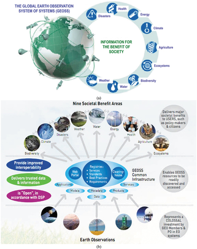
Table 2. Essential climate variables (ECVs) defined by the World Climate Organization (WCO) (Bojinski et al., 2014), pursued by the European Space Agency (ESA) Climate Change Initiative’s parallel projects (ESA – European Space Agency, 2017b, 2020a, 2020b) and by the Group on Earth Observations (GEO)’s second implementation plan for years 2016–2025 of the Global Earth Observation System of (component) Systems (GEOSS) (GEO – Group on Earth Observations, 2015; Nativi et al., 2015, 2020; Santoro et al., 2017), see Figure 1. In the terrestrial layer, ECVs are: River discharge, water use, groundwater, lakes, snow cover, glaciers and ice caps, ice sheets, permafrost, albedo, land cover (including vegetation types), fraction of absorbed photosynthetically active radiation, leaf area index (LAI), above-ground biomass, soil carbon, fire disturbance, soil moisture. All these ECVs can be estimated from Earth observation (EO) imagery by means of either physical or semi-empirical data models, e.g. Clever’s semi-empirical model for pixel-based LAI estimation from multi-spectral (MS) imagery (Van der Meer & De Jong, 2011).

Essential climate variables (ECVs) defined by the World Climate Organization (WCO) and pursued by the European Space Agency (ESA) Climate Change Initiative’s parallel projects
Atmospheric	Surface	Air temperature, wind speed and direction, water vapor, pressure, precipitation, surface radiation budget
	Upper air	Temperature, wind speed and direction, water vapor, cloud properties, Earth radiation budget (including solar irradiance)
	Composition	Carbon dioxide, methane, other long-lived greenhouse gases, ozone and aerosol supported by their precursors
Oceanic	Surface	Sea surface temperature, sea surface salinity, sea level, sea state, sea ice, surface current, ocean color, carbon dioxide partial pressure, ocean acidity, phytoplankton
	Subsurface	Temperature, salinity, current, nutrients, carbon dioxide partial pressure, ocean acidity, oxygen, tracers
Terrestrial	River discharge, water use, groundwater, lakes, snow cover, glaciers and ice caps, ice sheets, permafrost, albedo, land cover (including vegetation types), fraction of absorbed photosynthetically active radiation, leaf area index, above-ground biomass, soil carbon, fire disturbance, soil moisture

For example, in GEOSS, an important aspect related to property Value listed among the six Vs featured by EO big data is the identification, formalization and use of Essential (Community) Variables (Nativi et al., 2015, 2020; Santoro, Nativi, Maso, & Jirka, 2017). The Horizon 2020 ConnectinGEO project proposed a broad definition of Essential (Community) Variables (Santoro et al., 2017): “a minimal set of variables that determine the system’s state and developments, are crucial for predicting system developments, and allow us to define metrics that measure the trajectory of the system”. Intuitively, Essential (Community) Variables can be defined as EO sensory data-derived highly informative (high-level) variables, either numerical (continuous or discrete) or categorical (subsymbolic, semi-symbolic or symbolic, refer to this Section below), required for study, reporting, and management of real-world phenomena, related to any of the various components of the system Earth (e.g. oceans, land surface, solid Earth, biosphere, cryosphere, atmosphere and ionosphere) and their interactions (Nativi et al., 2020), in a specific scientific community and/or specific societal domain (Nativi et al., 2015, p. 18), including any of the nine “Societal Benefit Areas” targeted by GEOSS, namely, disasters, health, energy, climate, water, weather, ecosystems, agriculture and biodiversity, see Figure 1.

A popular community-specific ensemble of Essential (Community) Variables is that identified, formalized and adopted by the World Climate Organization (WCO) (Bojinski et al., 2014), whose Essential Climate Variables (ECVs) are either numerical or categorical, see Table 2. If numerical, then ECVs are always provided with a physical meaning, a physical unit of measure and a physical range of change, such as biophysical variables, e.g. leaf area index, above-ground biomass, etc. If categorical, then ECVs, specifically, land cover, are discrete, finite and symbolic (i.e. provided with meaning/semantics in a conceptual world model, refer to this Section below).

The ongoing GEO activity on the identification, formalization and use of EO sensory data-derived Essential (Community) Variables (such as ECVs, see Table 2) contributes to the process of making GEOSS an expert information and knowledge system, capable of EO sensory data interpretation/transformation into Essential (Community) Variables in support of decision making (Nativi et al., 2015, p. 18, 2020). It means that only high-level Essential (Community) Variables, rather than low-level EO big sensory data, should be delivered by GEOSS to end-users of spaceborne/airborne EO technologies for decision-making purposes. By focusing on the delivery to end-users of EO sensory data-derived Essential (Community) Variables as information sets relevant for decision-making, in place of delivering low-level EO big sensory data, the Big Data requirements of the GEOSS digital Common Infrastructure are expected to decrease (Nativi et al., 2015, p. 21, 2020), see Figure 1.

To take into account the fundamental difference between product/outcome and process/analytical pipeline, it is worth observing that term reusability in the FAIR principles for scientific digital data and non-data research objects management (see Table 1) is conceptually equivalent to tenet regularity adopted by the popular engineering principles of structured (data and information processing) system design, encompassing modularity, hierarchy and regularity (Lipson, 2007), considered neither necessary nor sufficient, but highly recommended for system scalability (Page-Jones, 1988).

To the same extent, term interoperability (opposite of heterogeneity) in the FAIR principles for scholarly/scientific digital data and non-data research objects (see Table 1) becomes, in the domain of analytical pipelines/processes, the tenet of data and information processing system (and/or component system, as functional unit) interoperability. System interoperability is typically defined as “the ability of systems to provide services to and accept services from other systems and to use the services so exchanged to enable them to operate effectively together” (Wikipedia, 2018). According to (ISO/IEC – International Organization for Standardization and International Electrotechnical Commission, 2015), system (and/or functional unit) interoperability is “the capability to communicate, execute programs, or transfer data among various functional units [component systems] in a manner that requires the user to have little or no knowledge of the unique characteristics of those units”; in short, it is “the capability of two or more functional units [component systems] to process data cooperatively”.

For example, the notion of “System of [component] Systems” proposed in GEOSS (see Figure 1) and the related “System of [component] Systems Engineering” process, “emerged in many fields of applications to address the common problem of [connecting and] integrating many [already existing or yet to be developed complex] independent autonomous systems, frequently of large dimensions, [each with its own objectives, requirements, mandate and governance], in order to satisfy a global [large-scale] goal [where component systems can leverage each other so that the overall System of Systems becomes much more than the sum of its component systems], while keeping [component systems] autonomous. System of [component] Systems can be usefully described as large-scale integrated systems that are heterogeneous and consist of [component] subsystems that are independently operable on their own, but are networked together for a common goal. System of [component] Systems Engineering solutions are necessary to address important challenges, such as: (i) Large-scale: in a System of [component] Systems, directing subsystems to a central task often introduces new challenging problems that for small systems may reduce the advantage of participating in a System of [component] Systems. Therefore, for small systems other solutions may be more effective and efficient. (ii) Heterogeneity: homogeneous/harmonized systems may be merged in an integrated system without the need of System of [component] Systems Engineering actions. (iii) Independent operability: the realization of a System of [component] Systems must not affect the normal and usual working of the composing systems. The System of [component] Systems Engineering needs to implement interoperability agreements supplementing without supplanting the existing ones. (iv) Effective networking: the composing [component] systems need to intercommunicate to achieve the common goal” (Nativi et al., 2015, p. 2).

To accomplish effective networking, in the terminology of GEOSS, a digital Common Infrastructure is required to allow end-users to search for and access to the interconnected component systems. To reach its goal, the GEOSS Common Infrastructure must rely upon a set of interoperability standards and best practices to interconnect, harmonize and integrate data, applications, models, and products of heterogeneous component systems (Nativi et al., 2015, p. 3), see Figure 1.

According to the existing literature, there are three levels of system interoperability (opposite of heterogeneity), corresponding to three generations of data and information processing systems.

• First lexical/communication level of system interoperability, involving computer system and data communication protocols, data types and formats, operating systems, transparency of location, distribution and replication of data, etc. (Sheth, 2015; Wikipedia, 2018).

• Second syntax/structural level of system interoperability. “Syntactic interoperability only focuses on the technical ability of systems to exchange data” (Hitzler et al., 2012). Intuitively, it is related to form, not content/ meaning/ semantics. According to Yingjie Hu, the term syntactics is in contrast with “the term semantics, which refers to the meaning of expressions in a language” (Hu, 2017). Syntactic interoperability of component systems is involved with query languages and user interfaces (Sheth, 2015; Wikipedia, 2018) at the two Marr levels of abstraction of an information processing system known as information/knowledge representation and structured system design (architecture) (Baraldi, 2017; Baraldi et al., 2018a, 2018b; Baraldi & Tiede, 2018a, 2018b; Marr, 1982; Quinlan, 2012; Sonka et al., 1994) (refer to the farther Subsection 3.2). For example, in traditional syntactic analysis (syntactic pattern recognition), a syntactic classifier assigns an input pattern (a word) to an appropriate class (of words) depending on whether or not that word can be generated by a class-specific grammar. When a class description grammar is regular, also known as type 3, then syntactic analysis is simple, because the grammar can be instantiated by a finite non-deterministic automaton (Sonka et al., 1994).

• Third semantic/ontological level of system interoperability (Baraldi, 2017; Baraldi & Tiede, 2018a, 2018b; Bittner, Donnelly, & Winter, 2005; Green, Bean, & Hyon Myaeng, 2002; Hitzler et al., 2012; Kuhn, 2005; Laurini & Thompson, 1992; Matsuyama & Hwang, 1990; Nativi et al., 2015, 2020; Obrst, Whittaker, & Meng, 1999; Sheth, 2015; Sonka et al., 1994; Sowa, 2000; Stock, Hobona, Granell, & Jackson, 2011; Wikipedia, 2018; Hu, 2017), which is increasingly domain-specific.

  In Kuhn (2005), semantic/ontological interoperability is considered the technical analogue to human communication and cooperation.

  As reported above, “the term semantics refers to the meaning of expressions in a language and is in contrast with the term syntactics” (Hu, 2017).

  For example, geospatial semantics is a recognized subfield in geographic information science (GIScience) (Buyong, 2007; Couclelis, 2010, 2012; Ferreira, Camara, & Monteiro, 2014; Fonseca, Egenhofer, Agouris, & Camara, 2002; Goodchild, Yuan, & Cova, 2007; Hitzler et al., 2012; Kuhn, 2005; Longley, Goodchild, Maguire, & Rhind, 2005; Maciel et al., 2018; Sheth, 2015; Sonka et al., 1994; Stock et al., 2011; Hu, 2017). In more detail, “geospatial semantics adds the adjective geospatial in front of semantics, and this addition both restricts and extends the initial applicable area of semantics. On one hand, geospatial semantics focuses on the expressions that have a connection with geography rather than any general expressions; on the other hand, geospatial semantics enables studies on not only linguistic expressions, but also the meaning/semantics of geographic places [in the physical world-domain] and geospatial data [in the domain of digital machines, like in Geographic Information Systems (GIS)]. Kuhn defines geospatial semantics as ‘understanding GIS contents, and capturing this understanding in formal theories’ (Kuhn, 2005). This definition can be divided into two parts: understanding and formalization. The understanding part triggers the question: who is supposed to understand the GIS content, people or machines? When the answer is “people”, research in geospatial semantics involves human cognition of geographic concepts and spatial relations; whereas when the answer is “machines”, it can involve research on the semantic interoperability of distributed systems, digital gazetteers, and geographic information retrieval. The second part of the definition proposes to capture this understanding through formal theories. Ontologies, as formal specifications of concepts and relations, have been widely studied and applied in geospatial semantics and formal logics, such as first-order logic and description logics, are often employed to define the concepts and axioms in an ontology [conceptual/ mental/ perceptual model of the world-domain of interest]. While Kuhn’s definition includes these two parts, research in geospatial semantics is not required to have both – one study can focus on understanding, while another one examines formalization” (Hu, 2017).

  Intuitively, “beyond the ability of two or more computer systems to exchange information [in compliance with the first lexical/communication level and the second syntax/structural level of system interoperability], semantic interoperability is the ability to automatically interpret the information exchanged meaningfully and accurately [i.e. to automatically and correctly understand the meaning/semantics of an exchanged message] in order to produce useful results as defined by the end users of both systems. To achieve semantic interoperability, both sides must refer to a common information exchange reference model” (Wikipedia, 2018), such as a world ontology, synonym for conceptual/ mental/ perceptual model of the 4D geospace-time physical world, to be agreed upon by members of a community before use by the community (Baraldi, 2017; Baraldi & Tiede, 2018a, 2018b; Green et al., 2002; Hitzler et al., 2012; Laurini & Thompson, 1992; Matsuyama & Hwang, 1990; Obrst et al., 1999; Sonka et al., 1994; Sowa, 2000; Stock et al., 2011). In other words, “[in a system of component systems, say, in an enterprise,] each system (or object of a system) can map from its own conceptual model [mental model of the world, world ontology] to the conceptual model of other systems, thereby ensuring that the meaning [semantics] of their information is transmitted, accepted, understood, and used across the enterprise” (Obrst et al., 1999). “The content [meaning, semantics] of the information exchange requests are unambiguously defined: what is sent is the same as what is understood” (Wikipedia, 2018).

  To guarantee semantic/ontological interoperability of component systems, “the subject of ontology is the study of the categories of things that exist or may exist in some domain. The product of such a study, called an ontology, is a catalog of the types of things that are assumed to exist in a domain of interest D from the perspective of a person who uses a language L for the purpose of talking about D“ (Sowa, 2000, p. 492). In an ontology, which is function of pair (D, L), “categories of things, expressed in L, that exist or may exist in an application domain, D, represent the ontological commitments of the ontology designer or knowledge engineer” (Sowa, 2000, p. 134). In practice, “ontologies are tools for specifying the semantics of terminology systems in a well-defined and unambiguous manner [community-agreed upon]. They are used to improve communication either between humans or computers by specifying the semantics [meaning] of the symbolic apparatus used in the communication process” (Bittner et al., 2005).

  In essence, “high-level semantic information availability reduces the problem of knowing the contents and structure of many sensory data and low-level information sources [at the first lexical/communication level or second syntax/structural level of system interoperability] to the problem of knowing the content of intuitive-to-use, high-level domain-specific (specialized) ontologies, which a [human] end-user familiar with the application domain is likely to know or understand easily” (Sheth, 2015), see Figure 2.

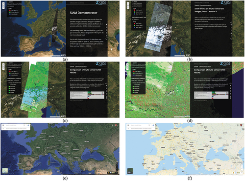
  Figure 2. Two examples of semantic/ontological interoperability over heterogeneous sensory data sources (true-facts, observables). The first example is provided by the demonstrator of the Satellite Image Automatic Mapper™ (SIAM™) lightweight computer program (Baraldi, 2017, 2019a; Baraldi et al., 2010a, 2010b, 2018a, 2018b; Baraldi, Puzzolo, Blonda, Bruzzone, & Tarantino, 2006; Baraldi & Tiede, 2018a, 2018b), installed onto the Serco ONDA Data and Information Access Services (DIAS) Marketplace (Baraldi, 2019a). This demonstrator works as proof-of-concept of an Artificial General Intelligence (AGI) (Bills, 2020; Chollet, 2019; Dreyfus, 1965, 1991, 1992; EC – European Commission, 2019; Fjelland, 2020; Hassabis et al., 2017; Ideami, 2021; Jajal, 2018; Jordan, 2018; Mindfire Foundation, 2018; Mitchell, 2021; Practical AI, 2020; Saba, 2020c; Santoro et al., 2021; Sweeney, 2018a; Thompson, 2018; Wolski, 2020a, 2020b), suitable for Earth observation (AGI4EO) applications, namely, ‘AGI for Data and Information Access Services (DIAS) = AGI4DIAS = AGI-enabled DIAS = Semantics-enabled DIAS 2.0 (DIAS 2^nd generation) = AGI + DIAS 1.0 + Semantic content-based image retrieval (SCBIR) + Semantics-enabled information/knowledge discovery (SEIKD)’ = Equation (1)(1) $\begin{array}{rl}& \text{lsquo}\mathrm{A}\mathrm{G}\mathrm{I}\text{-}\mathrm{e}\mathrm{n}\mathrm{a}\mathrm{b}\mathrm{l}\mathrm{e}\mathrm{d}\mathrm{D}\mathrm{I}\mathrm{A}\mathrm{S}=\mathrm{A}\mathrm{G}\mathrm{I}4\mathrm{D}\mathrm{I}\mathrm{A}\mathrm{S}=\mathrm{S}\mathrm{e}\mathrm{m}\mathrm{a}\mathrm{n}\mathrm{t}\mathrm{i}\mathrm{c}\mathrm{s}\text{-}\mathrm{e}\mathrm{n}\mathrm{a}\mathrm{b}\mathrm{l}\mathrm{e}\mathrm{d}\mathrm{D}\mathrm{I}\mathrm{A}\mathrm{S}2.0\\ & (\mathrm{D}\mathrm{I}\mathrm{A}\mathrm{S}{2}^{\mathrm{n}\mathrm{d}}\mathrm{g}\mathrm{e}\mathrm{n}\mathrm{e}\mathrm{r}\mathrm{a}\mathrm{t}\mathrm{i}\mathrm{o}\mathrm{n})=\mathrm{D}\mathrm{I}\mathrm{A}\mathrm{S}2.0=\mathrm{A}\mathrm{G}\mathrm{I}+\mathrm{D}\mathrm{I}\mathrm{A}\mathrm{S}1.0+\mathrm{S}\mathrm{C}\mathrm{B}\mathrm{I}\mathrm{R}+\mathrm{S}\mathrm{E}\mathrm{I}\mathrm{K}\mathrm{D}\text{rsquo}\end{array}$(1) , envisioned by portions of the existing literature (Augustin, Sudmanns, Tiede, & Baraldi, 2018; Augustin, Sudmanns, Tiede, Lang, & Baraldi, 2019; Baraldi, 2017; Baraldi & Tiede, 2018a, 2018b; Baraldi, Tiede, Sudmanns, Belgiu, & Lang, 2016; Baraldi, Tiede, Sudmanns, & Lang, 2017; Dhurba & King, 2005; FFG – Austrian Research Promotion Agency, 2015, 2016, 2018, 2020; Planet, 2018; Smeulders, Worring, Santini, Gupta, & Jain, 2000; Sudmanns, Augustin, van der Meer, Baraldi, and Tiede, 2021; Sudmanns, Tiede, Lang, & Baraldi, 2018; Tiede, Baraldi, Sudmanns, Belgiu, & Lang, 2017). In the present work, an integrated AGI4DIAS infrastructure = ‘AGI + DIAS 1.0 + SCBIR + SEIKD = DIAS 2.0ʹ is proposed as viable alternative to, first, traditional metadata text-based image retrieval systems, such as popular EO (raster-based) data cubes (Open Data Cube, 2020; Baumann, 2017; CEOS – Committee on Earth Observation Satellites, 2020; Giuliani et al., 2017, 2020; Lewis et al., 2017; Strobl et al., 2017), including the European Commission (EC) DIAS 1^st generation (DIAS 1.0) (EU – European Union, 2017, 2018), and, second, prototypical content-based image retrieval (CBIR) systems, whose queries are input with text information, summary statistics or by either image, object or multi-object examples (Datta, Joshi, Li, & Wang, 2008; Kumar, Berg, Belhumeur, & Nayar, 2011; Ma & Manjunath, 1997; Shyu et al., 2007; Smeulders et al., 2000; Smith & Chang, 1996; Tyagi, 2017). Typically, existing DIAS and prototypical CBIR systems are affected by the so-called data-rich information-poor (DRIP) syndrome (Ball, 2021; Bernus & Noran, 2017). Figure captions are as follows. (a) Mosaic of twenty-nine 12-band Sentinel-2 images, acquired across Europe on 19 April, 2019, radiometrically calibrated into top-of-atmosphere reflectance (TOARF) values, depicted in true-colors, 10 m resolution, equivalent to a QuickLook™ technology. (b) Mosaic of three 11-band Landsat-8 images acquired across Europe on 21 April, 2019, radiometrically calibrated into TOARF values, depicted in true-colors, 30 m resolution, equivalent to a QuickLook technology. (c) Overlap between two SIAM’s output maps in semi-symbolic color names (Baraldi, 2017, 2019a; Baraldi et al., 2010a, 2010b, 2018a, 2018b, 2006; Baraldi & Tiede, 2018a, 2018b), automatically generated in near real-time from, respectively, the input 10 m resolution Sentinel-2 image mosaic, shown in Figure 2(a), and the 30 m resolution Landsat-8 image mosaic shown in Figure 2(b). The same map legend applies to the two input data sets. Semantic (symbolic) interoperability is accomplished by SIAM, independent of the input data source. In practice, SIAM instantiates a QuickMap™ technology, where a categorical map, provided with its discrete and finite map legend, is sensory data-derived automatically, without human-machine interaction and in near real-time, either on-line or off-line. (d) Zoom-in of the two SIAM maps, featuring the same semantics, independent of changes in the input sensory data source. In practice, SIAM accomplishes semantic interoperability by featuring robustness to changes in input data and scalability to changes in sensor specifications. (e) Second example of semantic interoperability over heterogeneous sensory data sources. Taken from Google Earth = Google Maps_Satellite View, it is equivalent to a QuickLook technology. It shows multi-source sensory data (quantitative/unequivocal information-as-thing) (Baraldi & Tiede, 2018a, 2018b; Capurro & Hjørland, 2003), equivalent to subsymbolic numerical variables, to be interpreted by users. (f) Taken from Google Maps_Map View (qualitative/equivocal information-as-data-interpretation) (Baraldi & Tiede, 2018a, 2018b; Capurro & Hjørland, 2003), equivalent to a symbolic interpretation of Google Maps_Satellite View data. In practice, Google Maps_Map View works as QuickMap technology. To be run automatically and in near real-time, either on-line or off-line, a QuickMap technology accomplishes data compression through discretization/categorization, together with interpretation of a continuous or discrete numerical variable belonging to a (2D) image-plane into a discrete and finite categorical variable provided with semantics, belonging to an ontology (mental model, conceptual model) of the 4D geospace-time real-world (Baraldi, 2017; Baraldi & Tiede, 2018a, 2018b; Matsuyama & Hwang, 1990).

  

  For example, “in a multidisciplinary environment such as GEOSS, the semantic interoperability aspects acquire a particular importance. Different [component] systems may describe their resources according to different domain semantics. GEOSS addresses the resulting semantic heterogeneity consulting a set of interconnected and autonomous semantic assets, i.e. thesauri, controlled vocabularies and taxonomies” (Nativi et al., 2015, p. 13). In this regard, starting from 2016 as part of the new GEO’s task of developing an innovative GEOSS information and knowledge base, built upon the pre-existing GEOSS big data base, ”the definition, estimation and management of Essential (Community) Variables (see Table 2) helps semantic interoperability development in a significant way, by contributing to introduce a common lexicon and an unambiguous formalization of the features and behaviors of these variables for a given scope” (Nativi et al., 2020).

To ease the understanding of the aforementioned three levels of system interoperability, let us observe that the third semantic/ontological level of system interoperability appears related to the interoperability levels I1 and I2 of the FAIR guiding principles for scientific data (product and process) management (GO FAIR – International Support and Coordination Office, 2021; Wilkinson et al., 2016), see Table 1.

Moreover, it is worth recalling here that, in 2017, to create a Digital Single Market in Europe, where public administrations can collaborate digitally to develop seamless digital services and data flows, the European Commission (EC) proposed a European Interoperability Framework (EC – European Commission, 2021). The conceptual model of a European Interoperability Framework for an integrated public service governance, promoting the idea of “interoperability-by-design” as a standard approach for the design and operation of European public services, comprises four levels of interoperability: (i) legal interoperability, (ii) organizational interoperability, (iii) technical interoperability and (iv) semantic interoperability.

Intuitively, the third technical interoperability level of governance for an integrated public service promoted by the European Interoperability Framework encompasses the aforementioned first lexical/communication level and second syntax/structural level of system interoperability (Sheth, 2015; Wikipedia, 2018), while the fourth semantic interoperability level of governance of the European Interoperability Framework is one-to-one related to the aforementioned third semantic/ontological level of system interoperability (Bittner et al., 2005; Kuhn, 2005; Sheth, 2015; Sonka et al., 1994; Sowa, 2000; Wikipedia, 2018).

Independently of existing “concise, domain-independent, high-level principles [like FAIR or TRUST] that can be applied to a wide range of [scholarly/scientific digital data and non-data] research objects/outputs – from data [in the conventional sense] to analytical pipelines” (Wilkinson et al., 2016), the scientific attention of the present paper is totally focused on the semantic/ontological third-level of system interoperability to be accomplished by the ongoing research and technological development (RTD) of an innovative EO system of component systems, like GEOSS (see Figure 1), undertaken by the remote sensing (RS) meta-science community at the intergovernamental level of GEO in the last twenty years (refer to references listed in this Section above).

Like engineering, RS is a meta-science, i.e. it is an “applied” science of “basic” sciences (Wikipedia, 2020b). Its goal is to transform observations (sensory data, true-facts) of the physical 4D geospace-time real-world, together with information and knowledge about the world provided by other scientific disciplines, into useful (value-adding) user- and context-dependent information about the world and/or solutions in the world (Couclelis, 2012; Dreyfus, 1965, 1991, 1992; Fjelland, 2020).

According to Amit Sheth (2015), future data and information processing systems can become increasingly user- and domain-specific/ specialized/ “vertical”/ deep and narrow “minded” while accomplishing a third semantic/ontological level of system interoperability by linking (relating, associating, matching) automatically value-adding information, inferred from ever-varying sensory data, with a stable/hard-to-vary (Matsuyama & Hwang, 1990; Sweeney, 2018a) ontology (Bittner et al., 2005) of the 4D geospace-time physical world, also known as world model, mental model of the world or conceptual world model, available a priori and community-agreed upon (Baraldi, 2017; Baraldi & Tiede, 2018a, 2018b; Green et al., 2002; Laurini & Thompson, 1992; Matsuyama & Hwang, 1990; Sonka et al., 1994; Sowa, 2000).

By definition, a priori knowledge is any knowledge available before looking at sensory data/ observations/ true-facts, i.e. it is available in addition to (not as alternative to) sensory data or sensory data-derived information (Cherkassky & Mulier, 1998).

To the best understanding of the present authors, a “vertical”/ deep and narrow/ user- and application domain-specific stable/hard-to-vary conceptual/ mental/ perceptual model/ ontology of the 4D geospace-time physical world can be considered hierarchically built upon a more stable/harder-to-vary “horizontal”/ general-purpose/ user- and domain-independent commonsense knowledge base (Etzioni, 2017; Expert.ai, 2020; Thompson, 2018; U.S. DARPA – Defense Advanced Research Projects Agency, 2018; Wikipedia, 2021c), where the notion of commonsense knowledge can be one-to-one related to the notion of collective unconscious mind, which co-exists with the personal conscious mind in Jungian psychoanalysis. The former exists in all places, at all times, while the latter only exists in certain places at specific times (Hehe, 2021).

According to the existing literature, commonsense knowledge is referred to as “commonsense assumptions or default assumptions. It consists of facts about the everyday world that all humans are expected to know [without need for debate, such as ‘Lemons are sour’]” (U.S. DARPA – Defense Advanced Research Projects Agency, 2018). Oren Etzioni describes commonsense knowledge as all the weird, invisible, implied knowledge about the world that we all possess and take for granted, but rarely state out loud explicitly (Etzioni, 2017; Thompson, 2018). “It helps [humans] to solve [cognitive] problems in the face of incomplete information … As more knowledge of the world is discovered or learned over time, [the commonsense knowledge base of assumptions] can be revised, according to a truth maintenance process” (Wikipedia, 2021c). According to the U.S. Defense Advanced Research Projects Agency (DARPA), “possessing this essential background knowledge could significantly advance the symbiotic partnership between humans and machines [to be accomplished by a future Artificial General Intelligence, AGI, regarded by DARPA as human-level Artificial Intelligence, yet to be developed]. But articulating and encoding this obscure-but-pervasive capability is no easy feat … The absence of common sense prevents an intelligent system from understanding [the 4D geospace-time physical world of humans], communicating naturally with people, behaving reasonably in unforeseen situations, and learning from new experiences. This absence is perhaps the most significant barrier between the narrowly focused Artificial Intelligence applications [a.k.a. Artificial Narrow Intelligence, ANI = Equation (6)(6) $x0026;\text{ANI=}[\text{DCNN}\subset \text{DL}\subset \text{ML}\text{logical0OR}\text{Traditional}\text{deductive}ArtificialIntelligencex0026;(\text{static}\text{expert}\text{systems},\text{non0adaptive}\text{to}\text{data},\text{also}\text{known}\text{as}\text{Good}\text{Old0Fashioned}x0026;ArtificialIntelligence,\text{GOFAI}]$(6) , refer to this Section below] we have today and the more general Artificial Intelligence applications [a.k.a. Artificial General Intelligence, AGI = Equation (5)(5) $\text{lsquo}\mathrm{A}\mathrm{R}\mathrm{D}\subset \mathrm{E}\mathrm{O}\text{-}\mathrm{I}\mathrm{U}\subset \mathrm{C}\mathrm{V}\subset \mathrm{A}\mathrm{G}\mathrm{I}\leftarrow \mathrm{A}\mathrm{N}\mathrm{I}\leftarrow \mathrm{M}\mathrm{L}\supset \mathrm{D}\mathrm{L}\supset \mathrm{D}\mathrm{e}\mathrm{e}\mathrm{p}\mathrm{C}\mathrm{o}\mathrm{n}\mathrm{v}\mathrm{o}\mathrm{l}\mathrm{u}\mathrm{t}\mathrm{i}\mathrm{o}\mathrm{n}\mathrm{a}\mathrm{l}\mathrm{N}\mathrm{e}\mathrm{u}\mathrm{r}\mathrm{a}\mathrm{l}\mathrm{N}\mathrm{e}\mathrm{t}\mathrm{w}\mathrm{o}\mathrm{r}\mathrm{k}\left(\mathrm{D}\mathrm{C}\mathrm{N}\mathrm{N}\right)\text{rsquo}$(5) , refer to this Section below] we would like to create in the future” (U.S. DARPA – Defense Advanced Research Projects Agency, 2018).

One special case of present and/or future data and information processing systems (Sheth, 2015), required to link value-adding information, extracted from ever-varying sensory data, with a stable/hard-to-vary ontology of the 4D geospace-time physical world, which incorporates a commonsense knowledge base of assumptions, are computer vision (CV) systems, whose input data are a special case of sensory data, namely, imagery, synonym for 2D gridded data, belonging to a (2D) image-plane (Baraldi, 2017; Matsuyama & Hwang, 1990; Van der Meer & De Jong, 2011; Victor, 1994).

Encompassing both CV and biological vision, vision is an inherently ill-posed cognitive problem (sensory data interpretation task), whose goal is 4D geospace-time scene-from-(2D) image reconstruction and understanding (Baraldi, 2017; Matsuyama & Hwang, 1990), which requires, first, to cope with a data dimensionality reduction problem, from 4D of the world-domain to 2D of the image-domain, and, second, to fill the so-called semantic information gap, from ever-varying sensory data (numerical variables, specifically, sub-symbolic sensations) in the (2D) image-plane to stable percepts, equivalent to a discrete and finite set of concepts, provided with meaning/semantics (Ball, 2021; Capurro & Hjørland, 2003; Sowa, 2000) in a conceptual/ mental/ perceptual model/ ontology of the 3D observed scene (when acquisition time is fixed, in still imagery), which belongs to a 4D geospace-time physical world-domain (Augustin et al., 2018, 2019; Baraldi, 2017; Baraldi et al., 2018a, 2018b; Baraldi & Tiede, 2018a, 2018b; Baraldi et al., 2016, 2017; FFG – Austrian Research Promotion Agency, 2015, 2016, 2018, 2020; Matsuyama & Hwang, 1990; Sudmanns, Augustin, et al., 2021; Sudmanns et al., 2018; Tiede et al., 2017).

In a conceptual/ mental/ perceptual world model, dimensionality of the perceived 4D geospace-time real-world, observed and mapped (projected) onto a 2D image-plane by an imaging sensor involved with a cognitive visual process, is, apparently, 3D for geographic space (e.g. parameterized as latitude, longitude and height) (Hathaway, 2021) plus 1D for time (Ferreira et al., 2014; Fonseca et al., 2002; Galton & Mizoguchi, 2009; Maciel et al., 2018).

Actually, the 1D physical time dimension, synonym for 1D numerical variable of time, can be thought of/ perceived/ intellectually interpreted by humans (Buonomano, 2018; Harari, 2017; Hoffman, 2014; Otap, 2019). For example, in psychophysics, the well-known cold-water-through-time experiment conducted on human subjects apparently reveal that, in humans, two selves co-exist: every time our narrating self (verbal/symbolic left-brain hemisphere, which retrieves memories, provides meaning/semantics to experience/sensory data and makes decisions) evaluates/interprets our experiences sensed by the experiencing self (non-verbal/subsymbolic right-brain hemisphere, working as moment-to-moment sensoristic consciousness, which remembers nothing), the former is duration-blind. “Usually, it waves an experience using only peak moments and end results. The value of the whole experience is determined by averaging peaks with ends. It discounts [the experience] duration and adopts the peak-end rule” (Harari, 2017) (refer to this Section below).

Intuitively, a 1D physical time variable can be intellectually (mentally) discretized (categorized, stratified) into a discrete and finite categorical (nominal) variable (refer to the farther Subsection 3.3.1), consisting of three categorical values (categories, bins, strata, layers): past, present and future time, whose importance weights are different indeed. Typically, they are monotonically non-decreasing, from past to future. The future is never certain and can always change while the past remains the same. Actually, the past becomes increasingly fuzzy (foggy) and plastic in the memory through time. Recent series of experiments by psychologists show that people value events in the future more than they value equivalent events in the equidistant past, that they do so even when they consider this asymmetry irrational, and that one reason why they make these asymmetrical valuations is that contemplating future events produces greater affect than does contemplating past events (APS – Association for Psychological Science, 2008). While new studies in psychology explain why the future is more important than the past, as far as the power to create, the present is the most important time category. Actually, the future is collectively perceived as the most important time of the three time categories. For example, in recent years, the slogan of a political campaign of great success at national scale was “Hope” (for a better future). Intuitively, if I am subject to a dental treatment at present time, my endurance to an ever-varying sensation of pain benefits from my stable mental concept of hope in a better future.

From the previous paragraphs our conjecture is that, intuitively, whereas the sensory data dimensionality of an observed geospace-time scene-domain, belonging to the real (physical) world, is 3D for geographic space + 1D for time = 4D, the typical dimensionality of a stable/hard-to-vary (Matsuyama & Hwang, 1990; Sweeney, 2018a), but plastic (Baraldi & Alpaydin, 2002a, 2002b; Fritzke, 1997; Langley, 2012; Mermillod, Bugaiska, & Bonin, 2013; Wolski, 2020a, 2020b) conceptual/ mental/ perceptual model of the 4D geospace-time physical world is 7D overall, specifically:

• 3D for geographic space, e.g. Latitude, Longitude and Height. Plus

• 3D for time, partitioned for weighting purposes into past, present and future. Plus

• 1D for meaning-by-convention/semantics-in-context (Ball, 2021; Santoro et al., 2021; Sowa, 2000, p. 181), where meaning-by-convention/semantics-in-context is regarded as the conceptual/ mental/ intellectual meaning of observations of the real-world, provided by an interpretant. In agreement with philosophical hermeneutics (Capurro & Hjørland, 2003; Dreyfus, 1965, 1991, 1992; Fjelland, 2020), observation is synonym for true-fact (Matsuyama & Hwang, 1990), sensory data, sensation (Matsuyama & Hwang, 1990) or quantitative/unequivocal information-as-thing (Capurro & Hjørland, 2003). In agreement with philosophical hermeneutics (Capurro & Hjørland, 2003; Dreyfus, 1965, 1991, 1992; Fjelland, 2020) and semiotics (Ball, 2021; Peirce, 1994; Perez, 2020, 2021; Salad, 2019; Santoro et al., 2021; Wikipedia, 2021e), meaning-by-convention/semantics-in-context is synonym for percept (as mental result or product of perceiving) (Matsuyama & Hwang, 1990) or inherently ill-posed/ qualitative/ equivocal information-as-data-interpretation (Capurro & Hjørland, 2003) (for further details about meaning-by-convention/semantics-in-context as inherently ill-posed sign/ symbol/ data interpretation by an interpretant, refer to this Section below).

For the sake of completeness, let us observe that the proposed conceptualization of a mental world model as 7-dimensional cognitive space can be regarded as a simplification of the 11th dimension (Wikipedia, 2021f), which is a characteristic of spacetime that has been proposed as a possible answer to questions that arise in superstring theory/supergravity (Smolin, 2003), which involves the existence of 10 dimensions of space and 1 dimension of time. We see only three spatial dimensions and one time dimension, and the remaining seven spatial dimensions are “compactified”. According to Joshua Hehe, “I have found that by applying Ed Witten’s M-theory cosmology (Witten, 2001), which requires an 11-dimensional spacetime continuum, it becomes apparent to me that the three dimensions of open external space [geographic space] contain [physical] bodies while the seven dimensions of closed (‘compactified’) internal space must contain [the mind, related to the notion of personal conscious mind in Jungian psychoanalysis, which exists in certain geographic spaces at specific times, refer to this Section above]. What this means is that, along with these physical and mental state-spaces, I personally think that time serves as the dimension of interaction, thereby solving the mind-body problem. So, assuming my hypothesis is tenable, then the mechanism by which the mind affects the body is temporal in nature. This is true for the body affecting the mind, as well. In other words, the 3-dimensional objects in physical [external] space (dimensions 1–3) and the 7-dimensional [‘compactified’] subjects in metaphysical [mental, internal] space (dimensions 5–11) interact by way of time (dimension 4)” (Hehe, 2021).

If the physical dimension of time is threefold in human perception, then a natural question to ask might be the following (Capurro & Hjørland, 2003; Dreyfus, 1965, 1991, 1992; Fjelland, 2020).

In existing so-called Artificial Intelligence systems, expected to mimic and/or replace human behaviors and decision-making processes (EC - European Commission, 2019), what is the adopted model of time?

Interestingly enough, beyond their physical time, there is no (abstract, conceptual) model of time in typical artificial data and/or information processing systems, including so-called Artificial Intelligence systems.

The obvious observation (unquestionable true-fact) about these artificial systems/digital machines is that their being-in-the-world is by no means human-like (Capurro & Hjørland, 2003; Dreyfus, 1965, 1991, 1992; Fjelland, 2020). Hence, a natural question to ask might be the following.

If they are not in-the-world (of humans), how can artificial systems/digital machines reach human-level intelligence (Bills, 2020; Chollet, 2019; Dreyfus, 1965, 1991, 1992; Fjelland, 2020; Hassabis et al., 2017; Hawkins, 2021; Ideami, 2021; Jordan, 2018; Langley, 2012; Mindfire Foundation, 2018; Mitchell, 2021; Perez, 2017; Practical AI, 2020; Russell & Norvig, 1995; Saba, 2020c; Thompson, 2018; U.S. DARPA - Defense Advanced Research Projects Agency, 2018; Varela et al., 1991)?

According to Hubert Dreyfus, they cannot (Dreyfus, 1965, 1991, 1992), unless embodied cognition is pursued (Fjelland, 2020; Ideami, 2021; Mitchell, 2021; Perez, 2017; Varela et al., 1991) in the multi-disciplinary domain of cognitive science (Ball, 2021; Capra & Luisi, 2014; Hassabis et al., 2017; Hoffman, 2008, 2014; Langley, 2012; Miller, 2003; Mindfire Foundation, 2018; Mitchell, 2019; Parisi, 1991; Santoro et al., 2021; Serra & Zanarini, 1990; Varela et al., 1991; Wikipedia, 2019).

In the broad context of the scientific debate on the mind-brain problem (the French philosopher René Descartes is often credited with discovering the mind-body problem) (Hassabis et al., 2017; Hoffman, 2008; Serra & Zanarini, 1990; Westphal, 2016), cognitive science is the interdisciplinary scientific study focused on the mind and its (mental) processes (refer to references listed in the previous paragraph). To investigate cognitive (mental) processes, cognitive science encompasses disciplines like philosophy (Capurro & Hjørland, 2003; Dreyfus, 1965, 1991, 1992; Fjelland, 2020; Fodor, 1998; Peirce, 1994), semiotics (Ball, 2021; Peirce, 1994; Perez, 2020, 2021; Salad, 2019; Santoro et al., 2021; Wikipedia, 2021e), linguistics (Ball, 2021; Berlin & Kay, 1969; Firth, 1962; Rescorla, 2019; Saba, 2020a, 2020c), anthropology (Harari, 2011, 2017; Wikipedia, 2019), neuroscience (Barrett, 2017; Buonomano, 2018; Cepelewicz, 2021; Hathaway, 2021; Hawkins, 2021; Hawkins, Ahmad, & Cui, 2017; Kaufman, Churchland, Ryu, and Shenoy, 2014; Kosslyn, 1994; Libby & Buschman, 2021; Mason & Kandel, 1991; Salinas, 2021b; Slotnick, Thompson, & Kosslyn, 2005; Zador, 2019), which focuses on the study of the brain machinery in the mind-brain problem, computational neuroscience (Beniaguev, Segev, & London, 2021; DiCarlo, 2017; Gidon et al., 2020; Heitger, Rosenthaler, Von der Heydt, Peterhans, & Kubler, 1992; Pessoa, 1996; Rodrigues & Du Buf, 2009), psychophysics (Benavente, Vanrell, & Baldrich, 2008; Bowers & Davis, 2012; Griffin, 2006; Lähteenlahti, 2021; Mermillod et al., 2013; Parraga, Benavente, Vanrell, & Baldrich, 2009; Vecera & Farah, 1997), psychology (APS – Association for Psychological Science, 2008; Hehe, 2021), computer science (Sonka et al., 1994), formal logic (Laurini & Thompson, 1992; Sowa, 2000), mathematics, physics, statistics and (the meta-science of) engineering (Langley, 2012; Santoro et al., 2021; Wikipedia, 2019), which includes knowledge engineering (Laurini & Thompson, 1992) and GIScience (refer to references listed in this Section above). Cognitive science examines what cognition is, what it does and how it works (Wikipedia, 2019). It especially focuses on how information/knowledge is represented, acquired, processed and transferred either in the neuro-cerebral apparatus of living organisms or in machines, e.g. computers (Wikipedia, 2019) (also refer to Figure 11 in this Section below).

The notion of cognitive (mental) process involves thinking in the sense of Konrad Lorenz, i.e. acting in an imagined (mental) space (Lorenz, 1978; Schölkopf et al., 2021), synonym for acting in a 7D (refer to this Section above) conceptual/ mental/ perceptual model of the 4D geospace-time physical world, which agrees with a popular quote by Albert Einstein: “The true sign of intelligence is not knowledge, but imagination”, which allows to conduct “thinking experiments” (Salinas, 2021a).

In recent years, these enlightened intuitions have been supported by experimental evidence stemming from many research areas, pertaining to the multi-disciplinary domain of cognitive science. For example, according to neuroscience, at low-level cognitive (cortical) areas, when monkeys are preparing to move, neural activity in their motor cortex represents the potential movement (Cepelewicz, 2021). In other words, cortical activity in the null space permits preparation without movement (Kaufman, Churchland, Ryu, and Shenoy, 2014).

At higher cognitive levels, according to the research area of cognitive science called semantics, focused on linguistics and related to semiotics, “thinking in counterfactuals requires imagining a hypothetical reality that contradicts the observed facts, hence the name ‘counterfactual’. A counterfactual explanation describes a causal situation in the form: If [cause] X had not occurred, then [effect] Y would not have occurred” (Dandl & Molnar, 2021). It is a conditional statement, the first clause of which expresses something contrary to facts/observations, as “If I had known” (WordReference.com, 2021). In other words, a counterfactual is a hypothetical statement or question that cannot be verified or answered through observation (Heckerman & Shachter, 1995). In common practice, counterfactual inference enables humans to estimate the unobserved outcomes (Gonfalonieri, 2020). For example, “If I hadn’t taken a sip of this hot coffee, I wouldn’t have burned my tongue. Event Y is that I burned my tongue; cause X is that I had a hot coffee. The ability to think in counterfactuals makes us humans so smart compared to other animals” (Dandl & Molnar, 2021).

In line with the notion of counterfactual reasoning as hypothetical statement or question that cannot be verified or answered through observation (Heckerman & Shachter, 1995), Konrad Lorenz’ notion of thinking as acting in an imagined (mental) space (Lorenz, 1978) “ultimately requires the ability to reflect back on one’s actions and envision alternative scenarios, possibly necessitating (the illusion of) free will. The biological function of self-consciousness may be related to the need for a variable [a.k.a. agent] representing oneself in one’s Lorenzian imagined [mental] space, and free will may then be a means to communicate about actions taken by that variable, crucial for social and cultural learning, a topic which has not yet entered the stage of machine learning research although it is at the core of human intelligence” (Schölkopf et al., 2021).

According to Daniel Kahneman (Salinas, 2021a), “intelligence is not only the ability to reason [a.k.a logical thinking, based on understanding]; it is also the ability to find relevant material in memory”, for example, by means of the cognitive process of analogy (Marks, 2021; Mitchell, 2021), suitable for “hard” (inherently difficult) extrapolation (Ye, 2020) (refer to the farther Subsection 3.3.4). As Diego Salinas writes, “we all know intelligence has not a single component, it is a [mental] process made of many subtasks” (Salinas, 2021a), such as (mental) thinking as acting in one’s Lorenzian imagined (mental) space, focusing attention (for example, to filter out non-informative sensory data), logical reasoning, understanding (for example, understanding cause-effect relationships in the physical world), memory storage and recall capabilities, incremental learning as adaptation to changes in ever-varying sensory data (Baraldi & Alpaydin, 2002a, 2002b; Fritzke, 1997; Langley, 2012; Mermillod et al., 2013; Wolski, 2020a, 2020b), which requires both interpolation and extrapolation abilities (Gonfalonieri, 2020; Marks, 2021; Schölkopf et al., 2021; Ye, 2020), etc. “Some people excel in one of them, some at others” (Salinas, 2021a).

According to Diego Salinas (2021a), just like any other bodily function, human intelligence has evolved to keep us alive and therefore it takes many forms, i.e. it consists of many subtasks, to give us an advantage at a particular task. In 1972, Allen Newell and Herbert Simon, renown fathers of the Artificial (Narrow) Intelligence first golden age, typically referred to as Good Old-Fashioned Artificial Intelligence (GOFAI) (Dreyfus, 1965, 1991, 1992; Santoro et al., 2021) (refer to Equation (6)(6) $x0026;\text{ANI=}[\text{DCNN}\subset \text{DL}\subset \text{ML}\text{logical0OR}\text{Traditional}\text{deductive}ArtificialIntelligencex0026;(\text{static}\text{expert}\text{systems},\text{non0adaptive}\text{to}\text{data},\text{also}\text{known}\text{as}\text{Good}\text{Old0Fashioned}x0026;ArtificialIntelligence,\text{GOFAI}]$(6) in this Section below), wrote a seminal book (Newell & Simon, 1972) where they provided a well-known description of how human mind works. In summary (Salinas, 2021a), “they describe human intelligence as a process consisting of three stages.

1. Collecting information from the environment: if you could not perceive anything through your senses, you would not be able to acquire information. The ability to pay attention is the pipeline feeding your brain with food for thought.

2. Selecting criteria to take into account: this means using creativity [imagination, according to the two aforementioned quotes by Lorenz and Einstein] to think of all possible scenarios [conjectures, encompassing thinking in counterfactuals (Dandl & Molnar, 2021) and thinking by analogy (Marks, 2021; Mitchell, 2021), refer to this Section above], picture them in your mind and come up with the important factors related to the problem in question.

3. Choice: use logical reasoning to make a decision based on all available information”.

As much as your ability to run fast depends on many things like your legs length, body mass, running technique, etc., our ability to use intelligence depends on each of these components. So, broadly speaking, instead of “intelligence as a general concept”, Diego Salinas “prefers to talk about at least three different components that enhance each of these process stages: your ability to focus, your power of imagination, and your reasoning skills” (Salinas, 2021a).

In agreement with quotes reported in this Section above about the central role of imagination in human cognition/intelligence, Yuval Noah Harari believes that fictional mental abilities in human intelligence actually explain our mastery of planet Earth: “Homo sapiens is the only species on Earth capable of cooperating flexibly in large numbers. This concrete capability, rather than an eternal soul or some unique kind of self-consciusness or intelligence, explains our mastery of planet Earth. All large-scale social/cooperation networks, whose size, spatial extent and degree of flexibility go beyond those featured by small and local groups of individuals, whose cooperation is based on personal acquaintance and whose size/cardinality is typically not superior to 150 individuals, are ultimately based on community-agreed beliefs in new imagined [fictional, invented, virtual, mental] orders/realities, consisting of sets of fictional stories, rules, laws, places, entities or agents in history existing only in our common/shared imagination [mental world model], equivalent to neither objective entities [observables, true-facts, quantitative/unequivocal information-as-thing] nor subjective entities [based on personal sensations, emotions and beliefs, qualitative/ equivocal/ inherently ill-posed information-as-data-interpretation], but intersubjective entities to be shared/community-agreed upon in a triple-layered [mental model of] reality. Intersubjective entities depend on communication [and agreement] among many humans rather than on the subjective beliefs and feelings of individual humans. [Noteworthy, intersubjective entities, to be community-agreed upon, are conventional entities related to popular notions in semiotics, like meaning-by-convention (Santoro et al., 2021), equivalent to semantics-in-context (Ball, 2021)]. Examples of intersubjective entities of shared imagination, required to develop flexible large-scale human cooperation networks, are abstract/imagined notions (concepts) like gods, money, nations, corporations, etc. No other animal can stand up to Homo sapiens, not because they lack an eternal soul or a self-consciousness or mind, but because they lack the necessary imagination, the ability to create intersubjective entities that exist only in the shared imagination of large communities of individuals [as necessary-but-not-sufficient precondition to the development of flexible large-scale cooperation networks]. The humanity’s secret of success lies on the crucial importance of fictional intersubjective entities/realities [world models], which cannot be reduced to hormones and neurons. Hence, as well as separating humans from other animals, this mental ability to create intersubjective entities also separates the humanities from the life sciences, like neuroscience. If we want to understand and predict our future, cracking genomes and crunching numbers [big data] is hardly enough. We must also decipher the fictions [intersubjective entities] that give meaning [semantics] to the world” (Harari, 2017, pp. 153–182).

Worth observing, Harari’s fictional intersubjective entities/ realities/ world models, to be community-agreed upon as baseline knowledge suitable for keeping humans alive through flexible large-scale cooperation networks, naturally belong to the realm of commonsense knowledge (Etzioni, 2017; Expert.ai, 2020; Thompson, 2018; U.S. DARPA – Defense Advanced Research Projects Agency, 2018; Wikipedia, 2021c) (refer to this Section above).

Within the multi-disciplinary domain of cognitive science (refer to references listed in this Section above), according to neuroscience, the most recent and widely accepted theory about how emotions/ feelings/ sensations are created and experienced in human cognition is the theory of constructed emotions, developed by Lisa Feldman Barret (Barrett, 2017; Salinas, 2021b). She says that emotions “are not universal, but vary from culture to culture. They are not triggered; you create them. They emerge as a [personal, individual] combination of the physical properties of your body, a flexible brain that wires itself to whatever environment it develops in, and your culture and upbringing, which provide that environment” (Barrett, 2017). “In every waking moment, your brain uses past experience, organized as [discrete and finite, stable/hard-to-vary, but plastic] concepts, [where concepts in a conceptual world model can be two, say, like in ‘binary’ earthworn, or more than two, say, like in humans,] to guide your actions and give your sensations meaning. When the concepts involved are emotion concepts, your brain constructs instances of emotion [concepts], which is why it is called the theory of constructed emotion. It means that emotions are more than just a hardwired reflex [automatic, uncontrollable reaction] triggered by sensory inputs. Your emotions are created as a result of a combination of unique sensory inputs and the brain’s best predictions based on your individual experiences. In fact, your brain predictions’ anticipate sensory inputs such as vision or taste even before they happen. Then real sensory inputs either affirm the mind’s predictions as correct or wrong – if wrong, then the brain learns (updates) new predictions … This is the [plastic, dynamic] process of learning [a conceptual world model]” (Salinas, 2021b).

Moreover, in neuroscience, it is well known that, during every awaking moment, to make sense of their surroundings, to learn and to decide for action, humans and other animals combine mental representations of (present) perception with (past) memory. These living beings absorb new sensory information about the world around them while holding on to short-term memories of earlier observations or events. To avoid catastrophic interference between neural firing activity representations of perception and memory, their brain has to keep the two representations distinct. Otherwise, incoming data streams could interfere with representations of previous stimuli and cause these beings to overwrite or misinterpret important contextual information (Cepelewicz, 2021). Recent works in neuroscience show that, in mice, some populations of cortical neurons simultaneously process neural firing activity representations of short-term memories and sensations, while avoiding catastrophic interference between the two representations, such as catastrophic forgetting. To accomplish two overlapping neural activities without interference, the same population of cortical neurons adopts an orthogonal coding of the two neural firing activity representations. The brain rotates by 90 degrees representations of sensory information to be transformed into memories (Cepelewicz, 2021; Libby & Buschman, 2021). According to this emerging trend in neuroscience, populations of cortical neurons, even in lower parts of cortex such as sensory regions, are engaged in richer dynamic coding than was previously thought, where orthogonal coding of multiple information representations allows to combine information channels while protecting past information stored in buffers (Cepelewicz, 2021; Libby & Buschman, 2021). Short-term memory functions are not exclusively adopted by higher cognitive areas like the prefrontal cortex. Instead, the sensory regions and other lower cortical centers that detect and represent sensations and experiences may also encode and store memories of earlier observations or events. And yet those memories cannot be allowed to intrude on our perception of the present, or to be randomly rewritten by new experiences” (Cepelewicz, 2021).

So, the cognitive/mental process is not like this (Salinas, 2021b):

Sensory Input (I see a lion) → Emotion automatically triggered as uncontrollable reaction (I feel scared).

To the best understanding of the present authors, in agreement with works like (Barrett, 2017; Hawkins, 2021; Hawkins et al., 2017), whose focus is on the continuous ability of the brain to dynamically generate and update models of real-world objects and use those models (at the least, one binary/ Boolean/ two-value model) to predict sensory input and sensations/emotions, the cognitive/mental process might rather be like this:

(Conceptual/mental) Stable/hard-to-vary, but plastic concept (based on your individual genotype as initial condition + learning-from-examples phenotype/experience), related to (provided with) an expected/predicted (qualitative, subjective, ill-posed, ever-varying) physical/ bodily/ embodied Emotion/ Feeling/ Sensation + expected (quantitative) Sensory input, as concept-specific attributes → Prediction of Emotion/anticipated Emotion + Predicted/anticipated Sensory input ↔ Real-world sensory input → Prediction error in Sensory input → Emotion/ Feeling/ Sensation instance → Prediction error in Emotion → Either affirm or update concept, encompassing expected Emotion/ Feeling/ Sensation + expected Sensory input → Learning a conceptual/ mental/ perceptual model of the real-world.

As we move through the 3D geospace and/or 1D time dimensions of the 4D geospace-time physical world, we identify known objects and discover new objects. We continuously learn, generate and update our mental models of these objects as we observe new things about them (Daniels, 2021). As long as we are conscious, we are updating our mental models of the world objects. This is the very definition of “consciousness” in Jeff Hawkins’ theory, where the biological brain is explained as a continuously operating world modeling and prediction machine (Daniels, 2021; Hawkins, 2021).

In the view of the present authors, the well-known “boiling frog fable, describing a frog being slowly boiled alive” (Wikipedia, 2021g), provides an intuitive example of (biological) brain explained as a continuously operating world modeling and prediction machine, where a stable/hard-to-vary, but plastic (refer to references listed in this Section above) conceptual/ mental/ perceptual model of the 4D geospace-time physical world provides expected/predicted qualitative embodied sensations and/or quantitative sensory variables, to be compared with their instantaneous counterparts in the estimation of prediction errors, whose intensity drives the adaptivity of the internal conceptual world model to external change. In the “boiling frog fable, describing a frog being slowly boiled alive, the [actually, false] premise is that if a frog is put suddenly into boiling water, it will jump out, but if the frog is put in tepid water which is then brought to a boil slowly, it will not perceive the danger and will be cooked to death” (Wikipedia, 2021g). The story is often used as a metaphor for the inability or unwillingness of living beings to react to or be aware of gradual change-through-time in the (external) 4D geospace-time physical world, where change needs to be gradual in time to be accepted as change below a perceptual threshold of alarm/threat, although the overall change-through-time effect may increase in severity until reaching catastrophic proportions.

To explain the outcome of a well-known cold-water-through-time experiment conducted on human subjects, which replaces the popular metaphor of the boiling frog mentioned above, in his popular book, Yuval Noah Harari observes that “this experiment exposes the existence of at least two different selves: the experiencing self [non-verbal/subsymbolic right-brain hemisphere] and the narrating self [verbal/symbolic left-brain hemisphere]. The experiencing self is our moment-to-moment [sensoristic] consciousness … It remembers nothing [and is not consulted] when it comes to major decisions. Retrieving memories, telling stories [providing meaning/semantics to experience/sensory data] and making big decisions are all the monopoly of the narrating self. It is forever busy spinning yarns about the past and making plans for [and predictions about] the future. It does not narrate everything [and takes many shortcuts]. Usually, it waves the story using only peak moments and end results. The value of the whole experience is determined by averaging peaks with ends. Crucially, every time the narrating self evaluates our experiences, [it is duration-blind:] it discounts their duration and adopts the peak-end rule” (Harari, 2017).

In agreement with Peirce’s semiotics (Ball, 2021; Peirce, 1994; Perez, 2020, 2021; Santoro et al., 2021), encompassed by the multi-disciplinary domain of cognitive science (refer to references listed in this Section above), an interpretant incorporates the potential ambiguity in meaning/semantics of a message/substrate.

To our best understanding, inherent ambiguity of message/substrate interpretation is twofold. First, the conceptual/ mental/ perceptual world model is interpretant-dependent. Second, the interpreter has a pro-active role in understanding the context-dependent relationship, e.g. the conventional relationship, between a message/substrate and what it represents, specifically, in the terminology of semiotics (Ball, 2021; Peirce, 1994; Perez, 2020, 2021; Salad, 2019; Santoro et al., 2021; Wikipedia, 2021e), its meaning-by-convention/ semantics-in-context. A symbol consists of “some substrate – a scratch on a page, an air vibration, or an electrical pulse – that is imbued with meaning by matter of convention” (Santoro et al., 2021). Hence, “a symbol’s meaning is not intrinsic to its substrate, nor is it objective. Symbols are subjective entities” dependent on their context, devoid of meaning for the interpreter who does not participate in the established convention (Santoro et al., 2021) or context of utterance (Ball, 2021).

In the research area of cognitive science called semantics, focused on linguistics and related to semiotics, “many levels of meaning should be covered, such as the ambiguous meaning of words and phrases taken in isolation, through the meaning of an expression in a given context of utterance to communicate something” (Ball, 2021). For example, today’s linguistic interpreters represent knowledge differently from humans. “Today’s systems seek to store all possible words (signs/forms) in advance, while humans rely on what is called context of utterance. The science of semantics tells us the meaning of what people store. J. R. Firth called it ‘context of situation’ (Firth, 1962). People not only store the information (facts/opinions about the situation), but the full context that includes who said what, who heard it, when and where it was said, and other facts known at the time known as immediate and general common ground … A knowledge representation needs to include the information that people use to determine its validity” (Ball, 2021).

In summary, according to research areas in cognitive science focused on linguistics, such as semantics and semiotics, unlike today’s linguistic interpreters, human-level linguistic interpreters should map a vocabulary (actually, phrases) onto meaning-by-convention/ semantics-in-context (Ball, 2021; Santoro et al., 2021) by means of a mapping function which is inside of context (context-dependent), but language (message, substrate)-independent (Ball, 2021; Santoro et al., 2021).

In spite of this general knowledge in semantics and semiotics, when works in GIScience (refer to references listed in this Section above) started focusing on geospatial semantics, to investigate, for example, the role of geo-ontologies for semantic interoperability of services in geospatio-temporal databases (Hitzler et al., 2012; Kuhn, 2005; Stock et al., 2011; Hu, 2017), “it was assumed that each scientific discipline could agree on a domain-level ontology and that these ontologies could all refer back to one common foundational ontology. Lower level ontologies, e.g. application ontologies, were thought of as mere specializations of these ontologies. It turns out, however, that even within very specific domains it is difficult to get scientists to agree on a common definition for their domain vocabulary and especially to align these definitions with the very abstract and loaded classes from top-level ontologies. For instance, lenticular clouds can be classified as events or physical objects at the same time, feature types such as Hill can be specified as physical objects, features, or amount of matter, while these three classes are among the core distinctions proposed by foundational ontologies for physical endurants. In other terms, many types are multi-aspect phenomena to a degree where even top-level distinctions cannot be utilized without reference to context” (Hitzler et al., 2012).

In agreement with the notion of context of utterance/context of situation promoted by linguistics, it is well known by neuroscience that (as reported in this Section above) “during every waking moment, we humans and other animals have to balance on the edge of our awareness of past and present. We must absorb new sensory information about the world around us while holding on to short-term memories of earlier observations or events [regarded as contextual information]. Our ability to make sense of our surroundings, to learn, to act and to think all depend on constant, nimble interactions between perception and memory. But to accomplish this, the brain has to keep the two distinct; otherwise, incoming data streams could interfere with representations of previous stimuli and cause us to overwrite or misinterpret important contextual information” (Cepelewicz, 2021).

One practical consequence of the inherent ill-posedness of cognition as (mental) interpretation of a message/substrate (Capurro & Hjørland, 2003; Dreyfus, 1965, 1991, 1992; Fjelland, 2020), where the message/substrate is provided with meaning-by-convention/semantics-in-context by a message-to-meaning mapping function, which depends on (changes with) an interpretant-specific 7D conceptual world model, consisting of stable/hard-to-vary but plastic semantic elements, and an interpretant-specific knowledge of a context of utterance, was highlighted by John Ball, whose quote is: “Meaning/semantics allows ongoing generalization because it is rich content, not just labeled content. There can be many thousands of relations [of a message/substrate] to a referent [concept, entity, class of real-world objects] in a meaning layer, but [in the machine learning-from-data paradigm] data annotations [labeled data, supervised data, refer to the farther Subsection 3.3.3] may only capture a single feature for a particular purpose and unsupervised data [unlabeled data, refer to the farther Subsection 3.3.3] is limited to the content of the source files” (Ball, 2021).

To our best understanding, the notion of cognition, synonym for cognitive (mental, perceptual) process, traditionally investigated in the multi-disciplinary domain of cognitive science (refer to references listed in this Section above), is recapped as follows.

• In a community of (one or more) physical agents, whose (physical) domain of being is a physical world, W, a language, L, is adopted for the purpose of talking (communicating) about D, where D is a physical world-(sub)domain of interest (Sowa, 2000, p. 492), such that semantic relationhip ‘D ⊆ W’ holds, where symbol ‘⊆’ means specialization with inheritance from the superset (at right) to the subset, in agreement with symbols adopted by the standard Unified Modeling Language (UML) for graphical modeling of object-oriented software (Fowler, 2003).

• The goal of a cognitive (mental, perceptual) process accomplished by a physical agent, called interpretant, is qualitative/ equivocal/ inherently ill-posed (in the Hadamard sense) interpretation of a message/substrate in L (Capurro & Hjørland, 2003; Hadamard, 1902; Santoro et al., 2021).

• A message/substrate in L is either a conventional (qualitative) sign/ symbol/ form/ expression (Ball, 2021) (e.g. letter, word, phrase or nominal/categorical variable, refer to this Section below) or a quantitative/unequivocal numerical variable (continuous or discrete, refer to this Section below), e.g. sensory data sensed from ‘D ⊆ W’.

• Since an interpretant is a physical agent, whose (physical) domain of being is an interpretant-specific physical world, W, then, hypothetically, an interpretant can be either biological being or machine. The physical world-domain W of a biological interpretant is 4D geospace-time. The physical world-domain of a machine, W*, may or may not be human-like. For example, the physical world-domain of a not-embodied digital computer is not human-like (refer to references listed in this Section above). It means that human-like cognition is impossible to mimic by an artificial interpretant whose physical world-domain of being, W*, does not include the 4D geospace-time physical world-domain W of biological beings as special case, i.e. to mimic human-like cognition by machine, it is required that relationship ‘W* ⊇ W’ holds.

• To reach its goal, cognition implies different (mental, perceptual) capabilities (refer to this Section above).

• (Cognitive) interpretation of a message/substrate means to provide a message/substrate with meaning/semantics, where meaning/semantics in short must be understood as meaning-by-convention/semantics-in-context (Ball, 2021; Santoro et al., 2021).

• To be interpreted by an interpretant, a message/substrate is mapped onto (connected to, linked with) an interpretant-specific stable/hard-to-vary, but plastic (refer to references listed in this Section above) discrete and finite ensemble/ legend/ vocabulary/ taxonomy(D, L) of semantic elements (Ball, 2021)/ referents (Ball, 2021)/ classes of world-objects/ entities (Chen, 1976)/ concepts (Matsuyama & Hwang, 1990), encompassing low-level (subsymbolic) emotion concepts (Barrett, 2017; Salinas, 2021b).

• The cognitive forward (message-to-meaning, sensor-to-mind) mapping function of a message/substrate onto a discrete and finite taxonomy(D, L) of concepts is interpretant-specific. It is inside of context (context-dependent, convention-dependent), but language L (message/substrate)-independent (Ball, 2021; Santoro et al., 2021).

• A stable/hard-to-vary, but plastic taxonomy(D, L) of entities is part-without-inheritance-of an interpretant-specific stable/hard-to-vary, but plastic 7D (refer to this Section above) conceptual/ mental/ perceptual model/ ontology(D, L) of the interpretant-specific physical world-subdomain of interest, ‘D ⊆ W’.

• In addition to a discrete and finite taxonomy(D, L) of entities, an interpretant-specific conceptual/ mental/ perceptual model/ ontology(D, L) includes as part-of a stable/hard-to-vary, but plastic discrete and finite ensemble(D, L) of inter-class relationships/predicates, together with models of facts, events/occurrents and processes/phenomena in ‘D ⊆ W’ (refer to this Section below).

• To be used by members of a community of physical agents/interpretants, where language L is adopted for the purpose of talking about ‘D ⊆ W’, an interpretant-specific conceptual/ mental/ perceptual model/ ontology(D, L) must be community-agreed upon (Baraldi, 2017; Baraldi & Tiede, 2018a, 2018b; Matsuyama & Hwang, 1990).

To provide practical solutions to real-world cognitive (message-to-meaning) problems, knowledge engineering (Laurini & Thompson, 1992; Sowa, 2000) is the branch of the engineering meta-science (Couclelis, 2012) typically responsible of combining semantic information primitives to instantiate a conceptual/ mental/ perceptual model/ontology(‘D ⊆ W’, L), to be community agreed upon. These semantic information primitives are described as follows.

• Discrete objects/ individuals/ continuants in the world-(sub)domain of interest, ‘D ⊆ W’ (Ferreira et al., 2014; Fonseca et al., 2002; Galton & Mizoguchi, 2009; Maciel et al., 2018). They are defined as (perceived, mental) instances/individuals, either fictional (such as instances of Harari’s fictional intersubjective entities, refer to this Section above) or sensory data-derived, whose identity remains constant as they undergo changes in state, such as changes in entities/classes of real-world objects featuring that continuant as instance-of (Ferreira et al., 2014; Fonseca et al., 2002; Galton & Mizoguchi, 2009; Maciel et al., 2018; Tiede et al., 2017).

• Stable/hard-to-vary, but plastic discrete and finite ensemble/ legend/ vocabulary/ taxonomy(‘D ⊆ W’, L) of semantic elements/ referents/ entities/ concepts/ classes of objects/continuants (refer to this Section above). As such, a discrete and finite taxonomy(‘D ⊆ W’, L) of concepts is a nominal (categorical) variable in L (refer to the farther Subsection 3.3.1).

  Hence, there is always a discrete and finite vocabulary(‘D ⊆ W’, L) of entities as part-without-inheritance-of a stable/hard-to-vary, but plastic conceptual/ mental/ perceptual world model/ontology(‘D ⊆ W’, L). It means that a conceptual world ontology(‘D ⊆ W’, L) should never be confused with any of its parts, including taxonomy(‘D ⊆ W’, L).

  To be considered part-of a stable/hard-to-vary, but plastic conceptual world model/ontology(‘D ⊆ W’, L), a stable/hard-to-vary, but plastic discrete and finite taxonomy(‘D ⊆ W’, L) of classes of continuants is typically constrained as follows.

  • Mutually exclusive, in (the semantics of) D (Congalton & Green, 1999), see Figure 3.

    Figure 3. Adapted from (Ahlqvist, 2008; Di Gregorio, 2016; Di Gregorio & Jansen, 2000; Owers et al., 2021). Example of a standard land cover (LC) class taxonomy, developed by the geographic information science (GIScience) community (Buyong, 2007; Couclelis, 2010, 2012; Ferreira et al., 2014; Fonseca et al., 2002; Goodchild et al., 2007; Hitzler et al., 2012; Kuhn, 2005; Longley et al., 2005; Maciel et al., 2018; Sheth, 2015; Sonka et al., 1994; Stock et al., 2011; Hu, 2017). In conceptual terms, a taxonomy (legend) of LC classes is a hierarchical (multi-level, featuring inter-level parent-child relationships) vocabulary of entities (referents, classes of real-world objects) (Ball, 2021; Chen, 1976). Any LC class taxonomy is part-of a conceptual world model (world ontology, mental model of the world) (Baraldi, 2017; Baraldi & Tiede, 2018a, 2018b; Matsuyama & Hwang, 1990), consisting of entities (Ball, 2021; Chen, 1976), inter-entity relationships/predicates (Ball, 2021; Chen, 1976), facts (Campagnola, 2020), events/occurrents and processes/phenomena (Ferreira et al., 2014; Fonseca et al., 2002; Galton & Mizoguchi, 2009; Kuhn, 2005; Maciel et al., 2018; Tiede et al., 2017). Proposed by the Food and Agriculture Organization (FAO) of the United Nations (UN), the well-known hierarchical Land Cover Classification System (LCCS) taxonomy (Di Gregorio & Jansen, 2000) is two-stage and fully-nested. It consists of a first-stage fully-nested 3-level 8-class FAO LCCS Dichotomous Phase (DP) taxonomy, which is general-purpose, user- and application-independent. It consists of a sorted set of three dichotomous layers (Di Gregorio & Jansen, 2000): (i) Primarily Vegetated versus Primarily Non-Vegetated. In more detail, Primarily Vegetated applies to areas whose vegetative cover is at least 4% for at least two months of the year. Vice versa, Primarily Non-Vegetated areas have a total vegetative cover of less than 4% for more than 10 months of the year. (ii) Terrestrial versus aquatic. (iii) Managed versus natural or semi-natural. These three dichotomous layers deliver as output the following 8-class FAO LCCS-DP taxonomy. (A11) Cultivated and Managed Terrestrial (non-aquatic) Vegetated Areas. (A12) Natural and Semi-Natural Terrestrial Vegetation. (A23) Cultivated Aquatic or Regularly Flooded Vegetated Areas. (A24) Natural and Semi-Natural Aquatic or Regularly Flooded Vegetation. (B35) Artificial Surfaces and Associated Areas. (B36) Bare Areas. (B47) Artificial Waterbodies, Snow and Ice. (B48) Natural Waterbodies, Snow and Ice. The general-purpose user- and application-independent 3-level 8-class FAO LCCS-DP taxonomy is preliminary to a second-stage FAO LCCS Modular Hierarchical Phase (MHP) taxonomy, consisting of a battery of user- and application-specific one-class classifiers, equivalent to one-class grammars (syntactic classifiers) (Di Gregorio & Jansen, 2000). In recent years, the two-phase FAO LCCS taxonomy has become increasingly popular (Ahlqvist, 2008; Durbha et al., 2008; Herold et al., 2009, 2006; Jansen et al., 2008; Owers et al., 2021). For example, it is adopted by the ongoing European Space Agency (ESA) Climate Change Initiative’s parallel projects (ESA – European Space Agency, 2017b, 2020a, 2020b). One reason for its popularity is that the FAO LCCS hierarchy is “fully nested” while alternative LC class hierarchies, such as the Coordination of Information on the Environment (CORINE) Land Cover (CLC) taxonomy (Bossard et al., 2000), the U.S. Geological Survey (USGS) Land Cover Land Use (LCLU) taxonomy by J. Anderson (Lillesand & Kiefer, 1979), the International Global Biosphere Programme (IGBP) DISCover Data Set Land Cover Classification System (EC – European Commission, 1996) and the EO Image Librarian LC class legend (Dumitru et al., 2015), start from a first-level taxonomy which is already multi-class.

    

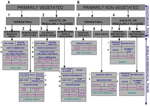
  • Totally exhaustive, in (the semantics of) D (Congalton & Green, 1999), see Figure 3.

  • Multi-level (hierarchical) in (the semantics of) D, where classes belonging to different hierarchical levels, i.e. classes at different levels of semantic granularity, are linked by parent-child relationships, synonym for relationship subset-of (specialization, with inheritance, also refer to this Section below), see Figure 3.

  These constraints are very familiar to the RS meta-science community, where D is the 4D geospace-time physical Earth (Ahlqvist, 2008; Bossard, Feranec, & Otahel, 2000; Congalton & Green, 1999; Di Gregorio & Jansen, 2000; Dumitru, Cui, Schwarz, & Datcu, 2015; Durbha, King, Shah, & Younan, 2008; EC – European Commission, 1996; ESA – European Space Agency, 2017b, 2020a, 2020b; Herold, Hubald, & Di Gregorio, 2009; Herold et al., 2006; Jansen, Groom, & Carrai, 2008; Lillesand & Kiefer, 1979; Owers et al., 2021).

  Fundamental properties of a taxonomy(‘D ⊆ W’, L) are cardinality/granularity (at the least equal to two, like in a binary/Boolean/two-value formal logic, or superior to two, like in typical crisp or fuzzy logics abopted by humans, where fuzzy sets are, for example, yes, no and maybe) and hierarchy (either flat or multi-level, to cope with semantic relationship subset-of, with inheritance), see Figure 3.

  Worth mentioning, in the Marr levels of system understanding (refer to the farther Subsection 3.2), the two taxonomical properties of semantic cardinality/granularity and hierarchy pertain to the second and third levels of system understanding, referred to as information/knowledge representation and system design (architecture). Hereafter, the two taxonomical properties of semantic granularity and hierarchy are further investigated.

  As reported in this Section above, it is well known in semiotics that message/substrate interpretation into meaning/semantics, to be regarded as meaning-by-convention/semantics-in-context (refer to references listed in this Section above), is a qualitative/equivocal information-as-data-interpretation process (Capurro & Hjørland, 2003), inherently ill-posed in the Hadamard sense (Hadamard, 1902) (refer to the farther Subsection 3.3.3).

  The inherent ill-posedness of information-as-data-interpretation means that, in the conceptualization of the physical world-domain of interest, D, according to terms provided by language L, there is no “universal” best semantic granularity (semantic resolution, vice versa, semantic scale), which is inversely related to the cardinality of the discrete and finite taxonomy of entities/classes of real-world objects required as part-of a conceptual world model (see Figure 3), exactly like there is no “universal” best number of bins for the discretization/ quantization/ categorization of a numerical variable into a categorical variable in vector quantization (VQ) problems (Baraldi & Alpaydin, 2002a, 2002b; Bishop, 1995; Cherkassky & Mulier, 1998; Fritzke, 1997).

  Since there is no “universal” semantic scale (vice versa, resolution) of analysis to conceptualize, in terms of language L, the real world-domain of interest, D, the only possible solution adopted in common practice by any community of interpretants is multi-scale hierarchical conceptualization of D. Hence, a vocabulary(D, L) of entities, to be community-agreed upon, is typically organized hierarchically, where hierarchical semantic/ontological levels of the vocabulary adopt, first, different degrees of semantic granularity, from coarse to fine, and, second, inter-level parent-child relationships, synonym for relationships superset-of (with inheritance) from a parent-entity to a child-entity, see Figure 3.

  Moreover, since semantic uncertainty is congenital in any information-as-data-interpretation task (Capurro & Hjørland, 2003), the semantic cardinality of a hierarchical vocabulary(D, L) of entities is N_l ≥ 2 at any hierarchical level l = 1, … ., L, where (N_l – 1) ≥ 1 is the number of target classes/ concepts/ entities at level l, while the N_l-th entity, required to cope with semantic uncertainty at hierarchical level l, is class “Unknown”/ “Others”/ “Outliers”/ “Rest of the world-domain of interest, D, at level l”. For example, in a one-class classification problem, N is equal to 2, according to a binary/Boolean/two-value formal logic.

  Constraint N_l ≥ 2 at any level l = 1, … ., L of a hierarchical vocabulary(D, L) of entities, where (N_l – 1) ≥ 1 is the number of target classes/ concepts/ entities at level l, while the N_l-th entity is class “Unknown at level l”, required to model semantic uncertainty at level l, is straightforward, but not trivial. It agrees with commonsense knowledge (refer to references listed in this Section above) and with traditional EO image classification system design and implementation requirements (Baraldi, 2017; Baraldi et al., 2018a, 2018b; Swain & Davis, 1978), where class “Unknown” (“Others”, “Outliers”) is considered mandatory to cope with (semantic) uncertainty in a vocabulary(D, L) of land cover (LC) classes of the Earth surface. Unfortunately, in the RS common practice, encompassing standard LC class taxonomies of the Earth surface, the proposed constraint is typically ignored, see Figure 3.

  In the realm of GIScience (refer to references listed in this Section above), well-known standard discrete and finite hierarchical taxonomies (vocabularies) of LC classes on the Earth surface, to be adopted as part-of a community-agreed conceptual model of the 4D geospace-time physical Earth, are the Coordination of Information on the Environment (CORINE) Land Cover (CLC) taxonomy (Bossard et al., 2000), the U.S. Geological Survey (USGS) Land Cover Land Use (LCLU) taxonomy by J. Anderson (Lillesand & Kiefer, 1979), the International Global Biosphere Programme (IGBP) DISCover Data Set Land Cover Classification System (EC – European Commission, 1996), the EO Image Librarian LC class legend (Dumitru et al., 2015), the two-stage fully-nested Food and Agriculture Organization (FAO) of the United Nations (UN) Land Cover Classification System (LCCS) taxonomy (see Figure 3), consisting of an 8-class 3-layer Dichotomous Phase (DP) taxonomy followed by a per-class Modular Hierarchical Phase (MHP) taxonomy (Ahlqvist, 2008; Di Gregorio, 2016; Di Gregorio & Jansen, 2000; Owers et al., 2021), etc.

• Stable/hard-to-vary, but plastic discrete and finite ensemble of inter-entity relationships/predicates (Ball, 2021; Chen, 1976), which is function of the adopted (D ⊆ W, L) pair, given a stable/hard-to-vary but plastic discrete and finite taxonomy(D, L) of entities.

  In the well-known formalism of set theory, a binary relationship R: A ⇒ B from set (entity of continuants) A, with cardinality |A| = a, and set (entity of continuants) B, whose cardinality |B| = b, is defined as any subset of the 2-fold Cartesian product between sets A and B, A × B. The Cartesian product of two sets, A × B, is a set whose elements are ordered pairs and whose size is rows × columns = a × b. In symbols, binary relationship R: A ⇒ B ⊆ A × B holds.

  Worth mentioning, in a conceptual world model, there are two peculiar categories (types) of inter-entity relationships. First, the so-called semantic relations (Green et al., 2002, p. 23), specifically, part-of without inheritance, like the part-whole relation meronymy, has-a, in WordNet, and subset-of (parent-child) with inheritance, like the super-subordinate relation hyperonymy, is-a, in WordNet (Ball, 2021; Green et al., 2002; Sonka et al., 1994; Sowa, 2000; WordNet, 2015).

  Second, causal (cause-effect) relationships. Causality is defined as “the influence by which one event, process or state, a cause, contributes to the production of another event, process or state, an effect, where the cause is partly responsible for the effect, and the effect is partly dependent on the cause” (Wikipedia, 2021b). Work by cognitive scientists, statisticians, and philosophers have emphasized the importance of identifying causal relationships for purposes of modeling the effects of actions (Heckerman & Shachter, 1995).

  Familiar to all human beings in their commonsense reasoning (Etzioni, 2017; Thompson, 2018; U.S. DARPA – Defense Advanced Research Projects Agency, 2018; Wikipedia, 2021c) and natural language understanding (Expert.ai, 2020; Rescorla, 2019; Saba, 2020a, 2020c), semantic and causal relations are peculiar because, like for grammar construction in traditional syntactic pattern recognition systems (Sonka et al., 1994, pp. 283–285), the learning process of semantic and causal relationships can rarely be algorithmic (statistical model-based) (Campagnola, 2020), i.e. they typically require significant human interaction (human-in-the-loop) (Wikipedia, 2021d) for information and knowledge representation (modeling) and processing system design (Sonka et al., 1994).

  In compliance with the well-known dictum that “cross-correlation does not imply causation” and vice versa (Baraldi, 2017; Baraldi & Soares, 2017; Fjelland, 2020; Gonfalonieri, 2020; Heckerman & Shachter, 1995; Kreyszig, 1979; Lovejoy, 2020; Pearl, 2009; Pearl et al., 2016; Pearl & Mackenzie, 2018; Schölkopf et al., 2021; Sheskin, 2000; Tabachnick & Fidell, 2014; Varando et al., 2021; Wolski, 2020a, 2020b), causal relationships should never be confused with cross-variable correlation functions, either linear or non-linear. For example, as reported in (Gonfalonieri, 2020), “in our projects, we try to not fall into the trap of equating correlation with causation.”

  In the words of Chris Lovejoy (Lovejoy, 2020), “a correlation is an association. When one thing goes up, another goes down. Or up. It doesn’t really matter, as long as they change together [or they do not change together]. But we don’t know whether the first change caused the second change. Or if the second cause the first. There could also be a third factor, which actually changes both points independently … and is the true cause of the correlation. Let’s say we notice a correlation between sunburn and ice cream sales. There’s a common cause for both; the sunny weather. Here, the sun is a ‘confounder’ (Pearl, 2009; Pearl et al., 2016) – something which impacts both variables of interest at the same time, leading to the correlation. So, in summary, to go from correlation to causation, we need to remove all possible confounders. If we control for all confounders (and account for random chance), and we still observe an association, we can say that there is causation. To remove confounders, the gold standard is the randomised control trial. Here, we divide our sample population into two, completely randomly. One half gets one treatment and one half gets another. Because the split was (at least in theory) completely random, any differences between outcome are down to the different treatment. If no randomised control trial is possible because, for example, we have already collected the data or we are investigating a variable we can’t change (like the impact of genetics, or the weather), a neat mathematical approach, called ‘stratifying on the confounders’, is proposed in (Pearl et al., 2016)”.

  Hans Reichenbach clearly articulated the connection between causality/causal explainibility (Sweeney, 2018a) and statistical dependence (Reichenbach, 1956; Schölkopf et al., 2021). He postulated the following (Reichenbach, 1956):

  Common Cause Principle: if two observables X and Y are statistically dependent, then there exists a variable Z [known as confounder (Heckerman & Shachter, 1995; Lovejoy, 2020; Pearl, 2009; Pearl et al., 2016)] that causally influences both and explains all the dependence in the sense of making them independent when conditioned on Z.

  It means that, “between causal and statistical structures, the more fundamental one is the causal structure, since it captures the physical mechanisms that generate statistical dependencies” (Schölkopf et al., 2021).

  To guarantee that two numerical variables are statistically independent, i.e. no cause-effect relationship holds between two numerical variables randomly sampled from a single population, the popular Pearson linear cross-correlation (PLCC) test (Kreyszig, 1979; Sheskin, 2000; Tabachnick & Fidell, 2014; Van der Meer & De Jong, 2011) is inadequate because it is well known that, first, PLCC is sensitive to linear relationships exclusively and, second, “cross-correlation does not imply causation” and vice versa. For example, it is easy to prove that PLCC(x, y) = cov(x, y)/[σ(x) ∙ σ(y)] = (E[x ∙ y] – E[x] ∙ E[y])/[σ(x) ∙ σ(y)] is equal to zero if y = x^2 with x in range [−1.0, 1.0], i.e. PLCC(x, y) can be zero when y is a non-linear deterministic (causal) function of x (Baraldi, 2017; Baraldi & Soares, 2017).

  In general, “nonlinearities, nonstationarities and the (ab)use of PLCC analyses hamper the discovery of true causal patterns” (Varando et al., 2021).

  The well-known Pearson Chi-square test of statistical independence can be applied when two categorical (nominal, discrete and finite) variables are randomly sampled from a single population (Kreyszig, 1979; Sheskin, 2000; Tabachnick & Fidell, 2014; U.S. EPA – Environmental Protection Agency, 1998). It is used to determine whether there is a significant association/ relation/ dependence between the two categorical variables, meaning that if the level (bin, bucket, interval) of the first nominal variable is known, then it can help predicting the level of the second nominal variable and vice versa.

  Indeed, quantization/ discretization/ binning of numerical variable pairs causes an irreversible loss of information, equivalent to a VQ (vector discretization/quantization) error (Baraldi & Alpaydin, 2002a, 2002b; Bishop, 1995; Cherkassky & Mulier, 1998; Fritzke, 1997): one cannot do the reverse of taking the categories and reproducing the raw quantitative (numerical) measurements. To avoid categorizing/discretizing numerical variables into a heuristic number of categories/ bins/ buckets/ intervals/ strata/ layers to apply the Pearson Chi-square test of independence, researchers and practitioners tend to (ab)use of PLCC analyses in the quest for causality among numerical patterns. To employ the Chi-square test of statistical independence, some researchers and practitioners undertake the discretization of numerical variables into a heuristic number of bins, e.g. take height measurements and categorize them into three levels, “below average”, “average”, and “above average”. Combining practicality with statistical soundness, a viable solution is an equiprobability Pearson Chi-Square test of statistical independence, where k equiprobable intervals must be selected (Baraldi & Soares, 2017; U.S. EPA – Environmental Protection Agency, 1998). A popular choice based on heuristics is: k = 2 * N^(2/5), where N is the size of the finite sample dataset (Baraldi & Soares, 2017; D’Agostino & Stephens, 1986; U.S. EPA – Environmental Protection Agency, 1998).

• Facts (Campagnola, 2020). A fact is typically represented as a Subject-Predicate-Object triple (Campagnola, 2020). For example, a continuant named Paul, whose identifier is Social Security Number 000–00-0018, owns the hammer whose identifier is Universal Product Code 009000 000001, where Paul is instance-of entity Citizens while the hammer at hand is instance-of entity Hardware Tools, where these two entities belong to a taxonomy of entitities, which is part-of a conceptual world ontology.

• Events/occurrents (Ferreira et al., 2014; Fonseca et al., 2002; Galton & Mizoguchi, 2009; Kuhn, 2005; Maciel et al., 2018; Tiede et al., 2017). An event/occurrent is defined as a relevant moment of change in state of one or more continuants. An event is always due to (caused by) a process/phenomenon.

• Processes/phenomena (Ferreira et al., 2014; Fonseca et al., 2002; Galton & Mizoguchi, 2009; Maciel et al., 2018; Tiede et al., 2017). A phenomenon, synonym for process or causal force, is identified by its causal effects, specifically, by an ensemble of one or more events.

In GIScience, among the aforementioned standard LC class taxonomies, to be considered mandatory as part-of a community-agreed conceptual world model, the two-stage fully-nested hierarchical FAO LCCS taxonomy (Ahlqvist, 2008; Di Gregorio, 2016; Di Gregorio & Jansen, 2000; Owers et al., 2021), originally proposed in year 2000 (see Figure 3), has been increasingly adopted by the RS meta-science community (Ahlqvist, 2008; Durbha et al., 2008; Herold et al., 2009, 2006; Jansen et al., 2008; Owers et al., 2021). For example, the FAO LCCS taxonomy is employed at the world spatial extent by the ongoing European Space Agency (ESA) Climate Change Initiative’s parallel projects (ESA – European Space Agency, 2017b, 2020a, 2020b), see Table 2.

The peculiar properties of the two-stage fully-nested hierarchical FAO LCCS taxonomy (see Figure 3) may explain its increasing popularity in the RS meta-science domain. In general, semantic error traceability is mandatory at each level of a LC class hierarchy (refer to this Section above) in compliance with:

1. The general-purpose garbage in, garbage out (GIGO) principle (Baraldi, 2017; Geiger et al., 2021; Thompson, 2018), which is intuitive to deal with, in agreement with commonsense knowledge (Etzioni, 2017; Expert.ai, 2020; Thompson, 2018; U.S. DARPA – Defense Advanced Research Projects Agency, 2018; Wikipedia, 2021c) (refer to this Section above).

2. The engineering principles of modularity, hierarchy and regularity, recommended for system scalability (Lipson, 2007).

3. The standard intergovernmental GEO-Committee on Earth Observation Satellites (CEOS) Quality Assurance Framework for Earth Observation (QA4EO) Calibration/Validation (Cal/Val) requirements (Baraldi, 2009; GEO-CEOS – Group on Earth Observations and Committee on Earth Observation Satellites, 2010; Schaepman-Strub, Schaepman, Painter, Dangel, & Martonchik, 2006; Shuai et al., 2020), where each step in a workflow must be validated by an independent third-party (GEO-CEOS, 2015) for quantitative quality assurance/traceability (vice versa, for error propagation and backtracking).

4. The Guide to the Expression of Uncertainty in Measurement (JCGM – Joint Committee for Guides in Metrology, 2008) and the International Vocabulary of Metrology (JCGM – Joint Committee for Guides in Metrology, 2012) issued by the Joint Committee for Guides in Metrology.

In a LC class hierarchy, mandatory semantic error traceability is maximum (refer to this Section above) if the class hierarchy is “fully nested”, to maximize its number of layers, like in the FAO LCCS two-stage DP and MHP taxonomy (Di Gregorio & Jansen, 2000) (see Figure 3), which would explain its increasing popularity. Semantic error traceability is inferior in LC class taxonomies which are not “fully nested” because their first-level taxonomy is already multi-class, such as the aforementioned CORINE CLC taxonomy (Bossard et al., 2000), the USGS LCLU taxonomy by J. Anderson (Lillesand & Kiefer, 1979), the IGBP DISCover Data Set Land Cover Classification System (EC – European Commission, 1996) and the EO Image Librarian LC class legend (Dumitru et al., 2015).

Last but not least, about any conceptual world model to be transmitted to/shared by members of a community before and/or after being community-agreed upon, it is worth recalling here that a hypergraph-based data structure formalism (Laurini & Thompson, 1992, p. 456) allows a hierarchical graphical representation of a conceptual world model (Matsuyama & Hwang, 1990). A graphical representation of a conceptual ontology of a real world-domain of interest, D, conceptualized by a community in the terms of a language, L, is known as semantic data model (Laurini & Thompson, 1992), semantic net (Sonka et al., 1994, p. 259), semantic network (Sowa, 2000, p. 4), conceptual network (Baraldi, 2017; Growe, 1999; Liedtke, Bückner, Grau, Growe, & Tönjes, 1997), model graph (Sonka et al., 1994, p. 293), conceptual graph (Sowa, 2000, p. 181), knowledge representation system (Green et al., 2002, p. 93), or knowledge graph (Campagnola, 2020; Expert.ai, 2020; Futia, 2020; ODSC – Open Data Science, 2018; Perera, 2021).

In a traditional semantic network, entities are graphically represented as nodes and inter-entity relationships as arcs between nodes. An event/occurrent is typically depicted as an edge in a state diagram/ graph of states/ state graph (Wikipedia, 2017). A process/phenomenon is typically depicted as node in a flow chart/ workflow/ program graph (Wikipedia, 2017).

Hence, a conceptual world model can be graphically represented as a traditional semantic (conceptual) network with entities as nodes and relationships as arcs between nodes, augmented with the classic form of, first, a finite-state diagram for event modeling as change in state and, second, a finite program graph/flow chart for process modeling (Baraldi, 2017; Tiede et al., 2017). Noteworthy, processes are nodes in flow charts corresponding to edges in state diagrams. A program graph/flow chart and a finite-state diagram can be merged to form a Petri net (Wikipedia, 2013), also known as place/transition net, which is more general than either of them (Sowa, 2000, p. 218).

In the present work, while hiding lexical/communication and syntax/structural levels of system interoperability, semantic/ontological interoperability of component systems is regarded as necessary-but-not-sufficient precondition of semantics-enabled high-level information queries, such as queries suitable for semantic content-based image retrieval (SCBIR) and semantics-enabled information/knowledge discovery (SEIKD), envisioned by portions of the existing literature (Augustin et al., 2018, 2019; Baraldi, 2017; Baraldi & Tiede, 2018a, 2018b; Baraldi et al., 2016, 2017; Dhurba & King, 2005; FFG – Austrian Research Promotion Agency, 2015, 2016, 2018, 2020; Planet, 2018; Smeulders et al., 2000; Sudmanns, Augustin, et al., 2021; Sudmanns et al., 2018; Tiede et al., 2017), see Figure 2.

Intuitive to deal with by human operators because consistent with symbolic human reasoning (Newell & Simon, 1972) formulated in natural language, synonym for human-speak, alternative to techno-speak (Brinkworth, 1992), SCBIR and SEIKD capabilities would support a query like (see Figure 2): in a large EO image database management system, required to cope with the six Vs of EO big data, namely, volume, variety, veracity, velocity, volatility and value (Metternicht et al., 2020), retrieve all EO images where a flooding event occurs through time within a urban area detected across:

1. Low-level multi-sensor (heterogeneous) uncalibrated sensory data (true-facts, observables), synonym for dimensionless numerical variables provided with no physical meaning (Baraldi, 2009; Pacifici, Longbotham, & Emery, 2014), i.e. featuring no physical unit of measure, such as multi-sensor EO optical and synthetic aperture radar (SAR) Level 0 imagery in dimensionless digital numbers (DNs), stored as unstructured data (without label/annotation) (Ball, 2021; Rowley, 2007; Stanford University, 2020; Wikipedia, 2020a)/ unsupervised data/ unlabeled data (Bishop, 1995; Cherkassky & Mulier, 1998), in raster graphics formats in (2D) bitmap-domain/ image-domain/ dot matrix data structure-domain/ 2D gridded data-domain. And/or

2. Low-level sensory data-derived calibrated numerical variables, provided with a physical meaning, a physical unit of measure and a physical range of change, either continuous (uncountable) or discrete (countable), known as geo-fields in the (2D) image-plane (Couclelis, 2010; Goodchild et al., 2007), stored as unstructured data in raster graphics formats. They include, for example: (a) EO sensory data-derived numerical variables provided with a physical unit of radiometric measure, e.g. EO Level 1 imagery radiometrically calibrated into top-of-atmosphere reflectance (TOARF) values in the physical range of change [0.0, 1.0] (Baraldi, 2009; Baraldi et al., 2014; DigitalGlobe, 2017; Helder et al., 2018). (b) Biophysical Earth surface variables, such as those included in the list of terrestrial ECVs defined by the WCO, see Table 2. For example, a scalar wind-speed estimate in meter per second or a vegetation LC class-conditional leaf area index (LAI), which is a pure (dimensionless) non-negative real value ≥ 0 provided with a physical meaning, see Table 2. Representing the non-negative amount of leaf material in an ecosystem, LAI is physically defined as the total one-sided area (in square meter) of photosynthetic tissue per unit ground surface area (in square meter) (Liang, 2004). Hence, LAI is LC class-conditioned (stratified, masked), it is equal to zero where vegetated LC classes are absent. And/or

3. (Mid-level) sensory data-derived subsymbolic categorical variables, known as field-objects in the (2D) image-plane (Couclelis, 2010; Goodchild et al., 2007), to be stored as unstructured data in either raster or vector graphics formats (Arocena, Lozano, Quartulli, Olaizola, & Bermudez, 2015; Tran, Aussenac-Gilles, Comparot, & Trojahn, 2020). They include discrete and finite fuzzy sets, e.g. “high”, “medium” or “low” (discretized membership functions), of a geospatial numerical variable (Zadeh, 1965). For example, a Digital Elevation Model (DEM) is partitioned into three strata (layers, categories), where elevation values are discretized as fuzzy sets “high”, “medium” or “low”. And/or

4. High-level sensory data-derived symbolic instances, corresponding to discrete and finite real-world objects/continuants in the 4D world-domain (refer to this Section above), known as discrete and finite geo-objects in the (2D) image-plane (Couclelis, 2010; Goodchild et al., 2007). They are stored as organized or structured data (Rowley, 2007; Wikipedia, 2020a)/ supervised data/ labeled data (Bishop, 1995; Cherkassky & Mulier, 1998)/ annotated data/ interpreted data (Ball, 2021; Stanford University, 2020), in vector graphics formats in the (2D) image-domain (Arocena et al., 2015; Tran et al., 2020). They belong to a community-agreed discrete and finite set (taxonomy, vocabulary, legend) of symbolic (categorical and semantic) variables (for example, see land cover in the list of terrestrial ECVs shown in Table 2), where each symbolic variable is an entity/class of real-world objects in a 7D conceptual world model (refer to this Section above), see Figures 2 and 3.

Two intuitive examples of semantic interoperability accomplished by symbolic information products, generated either manually by humans or semi-automatically or automatically by machines from heterogeneous big sensory data sources (equivalent to true-facts, observables), are shown in Figure 2. The first example is provided by the demonstrator of the Satellite Image Automatic Mapper™ (SIAM™) lightweight computer program (Baraldi, 2017, 2019a; Baraldi et al., 2010a, 2010b, 2018a, 2018b, 2006; Baraldi & Tiede, 2018a, 2018b), installed onto the Serco ONDA Data and Information Access Services (DIAS) Marketplace (Baraldi, 2019a). This demonstrator works as proof-of-concept of an Artificial General Intelligence (AGI), also known as Artificial Broad/Strong Intelligence (Bills, 2020; Chollet, 2019; Dreyfus, 1965, 1991, 1992; EC – European Commission, 2019; Fjelland, 2020; Hassabis et al., 2017; Ideami, 2021; Jajal, 2018; Jordan, 2018; Mindfire Foundation, 2018; Practical AI, 2020; Romero, 2021; Santoro et al., 2021; Sweeney, 2018a; Wolski, 2020a, 2020b), for Earth observation (AGI4EO) applications, where conjecture

(1) $\begin{array}{rl}& \text{lsquo}\mathrm{A}\mathrm{G}\mathrm{I}\text{-}\mathrm{e}\mathrm{n}\mathrm{a}\mathrm{b}\mathrm{l}\mathrm{e}\mathrm{d}\mathrm{D}\mathrm{I}\mathrm{A}\mathrm{S}=\mathrm{A}\mathrm{G}\mathrm{I}4\mathrm{D}\mathrm{I}\mathrm{A}\mathrm{S}=\mathrm{S}\mathrm{e}\mathrm{m}\mathrm{a}\mathrm{n}\mathrm{t}\mathrm{i}\mathrm{c}\mathrm{s}\text{-}\mathrm{e}\mathrm{n}\mathrm{a}\mathrm{b}\mathrm{l}\mathrm{e}\mathrm{d}\mathrm{D}\mathrm{I}\mathrm{A}\mathrm{S}2.0\\ & (\mathrm{D}\mathrm{I}\mathrm{A}\mathrm{S}{2}^{\mathrm{n}\mathrm{d}}\mathrm{g}\mathrm{e}\mathrm{n}\mathrm{e}\mathrm{r}\mathrm{a}\mathrm{t}\mathrm{i}\mathrm{o}\mathrm{n})=\mathrm{D}\mathrm{I}\mathrm{A}\mathrm{S}2.0=\mathrm{A}\mathrm{G}\mathrm{I}+\mathrm{D}\mathrm{I}\mathrm{A}\mathrm{S}1.0+\mathrm{S}\mathrm{C}\mathrm{B}\mathrm{I}\mathrm{R}+\mathrm{S}\mathrm{E}\mathrm{I}\mathrm{K}\mathrm{D}\text{rsquo}\end{array}$(1)

holds in practice as our working hypothesis, envisioned by portions of the existing literature (refer to references listed in this Section above), see Figure 2.

Hereafter, an integrated AGI4DIAS solution = ‘AGI + DIAS 1.0 + SCBIR + SEIKD = DIAS 2.0’ = Equation (1)(1) $\begin{array}{rl}& \text{lsquo}\mathrm{A}\mathrm{G}\mathrm{I}\text{-}\mathrm{e}\mathrm{n}\mathrm{a}\mathrm{b}\mathrm{l}\mathrm{e}\mathrm{d}\mathrm{D}\mathrm{I}\mathrm{A}\mathrm{S}=\mathrm{A}\mathrm{G}\mathrm{I}4\mathrm{D}\mathrm{I}\mathrm{A}\mathrm{S}=\mathrm{S}\mathrm{e}\mathrm{m}\mathrm{a}\mathrm{n}\mathrm{t}\mathrm{i}\mathrm{c}\mathrm{s}\text{-}\mathrm{e}\mathrm{n}\mathrm{a}\mathrm{b}\mathrm{l}\mathrm{e}\mathrm{d}\mathrm{D}\mathrm{I}\mathrm{A}\mathrm{S}2.0\\ & (\mathrm{D}\mathrm{I}\mathrm{A}\mathrm{S}{2}^{\mathrm{n}\mathrm{d}}\mathrm{g}\mathrm{e}\mathrm{n}\mathrm{e}\mathrm{r}\mathrm{a}\mathrm{t}\mathrm{i}\mathrm{o}\mathrm{n})=\mathrm{D}\mathrm{I}\mathrm{A}\mathrm{S}2.0=\mathrm{A}\mathrm{G}\mathrm{I}+\mathrm{D}\mathrm{I}\mathrm{A}\mathrm{S}1.0+\mathrm{S}\mathrm{C}\mathrm{B}\mathrm{I}\mathrm{R}+\mathrm{S}\mathrm{E}\mathrm{I}\mathrm{K}\mathrm{D}\text{rsquo}\end{array}$(1) is proposed as innovative, but viable alternative to, first, traditional metadata text-based image retrieval systems, such as popular EO (raster-based) data cubes (Open Data Cube, 2020; Baumann, 2017; CEOS – Committee on Earth Observation Satellites, 2020; Giuliani et al., 2017, 2020; Lewis et al., 2017; Strobl et al., 2017), including the EC DIAS 1^st generation (DIAS 1.0) (EU – European Union, 2017, 2018), and, second, prototypical content-based image retrieval (CBIR) systems, whose queries are input with text information, summary statistics or by either image, object or multi-object examples (Datta et al., 2008; Kumar et al., 2011; Ma & Manjunath, 1997; Shyu et al., 2007; Smeulders et al., 2000; Smith & Chang, 1996; Tyagi, 2017), see Figure 4.

Figure 4. Adapted from (Tyagi, 2017). Typical architecture of a content-based image retrieval (CBIR) system (Datta et al., 2008; Kumar et al., 2011; Ma & Manjunath, 1997; Shyu et al., 2007; Smeulders et al., 2000; Smith & Chang, 1996; Tyagi, 2017), whose prototypical instantiations have been presented in the remote sensing (RS) and computer vision (CV) literature as an alternative to traditional metadata text-based image retrieval systems in operational mode (Airbus, 2018; Planet, 2017). CBIR system prototypes support no semantic CBIR (SCBIR) operation because they lack ‘Computer Vision (CV) ⊃ EO image understanding (EO-IU)’ capabilities, i.e. they lack “intelligence” required to transform EO big sensory data into systematic, operational, timely and comprehensive information-as-data-interpretation (Capurro & Hjørland, 2003), known that relationship ‘EO-IU ⊂ CV ⊂ Artificial General Intelligence (AGI) ⊂ Cognitive science’ = Equation (2)(2) $\text{lsquo}\mathrm{C}\mathrm{o}\mathrm{g}\mathrm{n}\mathrm{i}\mathrm{t}\mathrm{i}\mathrm{v}\mathrm{e}\mathrm{s}\mathrm{c}\mathrm{i}\mathrm{e}\mathrm{n}\mathrm{c}\mathrm{e}\supset \mathrm{A}\mathrm{G}\mathrm{I}\supset \mathrm{C}\mathrm{V}\supset \mathrm{E}\mathrm{O}\text{-}\mathrm{I}\mathrm{U}\text{rsquo}$(2) holds (Bills, 2020; Chollet, 2019; Dreyfus, 1965, 1991, 1992; EC – European Commission, 2019; Fjelland, 2020; Hassabis et al., 2017; Ideami, 2021; Jajal, 2018; Jordan, 2018; Mindfire Foundation, 2018; Mitchell, 2021; Practical AI, 2020; Saba, 2020c; Santoro et al., 2021; Sweeney, 2018a; Thompson, 2018; Wolski, 2020a, 2020b).

Existing EO big data management systems, including DIAS and prototypical CBIR systems (see Figure 4), are typically affected by the so-called data-rich information-poor (DRIP) syndrome (Bernus & Noran, 2017). In short, “what is missing from data science is meaning [semantics]” (Ball, 2021). Intuitively, traditional EO big data management systems are affected by the DRIP syndrome because they lack an integrated ‘AGI ⊃ CV ⊃ EO image understanding (EO-IU)’ system in operational mode (refer to this Section below), suitable for transforming large EO image databases, acquired in the 4D geospace-time physical world-domain and characterized by the six Vs of volume, variety, veracity, velocity, volatility and value (Metternicht et al., 2020), into systematic, operational, timely and comprehensive value-adding information products and services (VAPS), starting from semantic (symbolic) information products, such as the well-known ESA EO Sentinel-2 image-derived Level 2 Scene Classification Map (SCM) co-product (DLR – Deutsches Zentrum für Luft-und Raumfahrt e.V. and VEGA Technologies, 2011; ESA – European Space Agency, 2015).

The aforementioned relationship ‘AGI ⊃ CV ⊃ EO-IU’ holds true in the multi-disciplinary domain of cognitive science (refer to references listed in this Section above). In more detail (also refer to Figure 11 in this Section below), semantic relationship

(2) $\text{lsquo}\mathrm{C}\mathrm{o}\mathrm{g}\mathrm{n}\mathrm{i}\mathrm{t}\mathrm{i}\mathrm{v}\mathrm{e}\mathrm{s}\mathrm{c}\mathrm{i}\mathrm{e}\mathrm{n}\mathrm{c}\mathrm{e}\supset \mathrm{A}\mathrm{G}\mathrm{I}\supset \mathrm{C}\mathrm{V}\supset \mathrm{E}\mathrm{O}\text{-}\mathrm{I}\mathrm{U}\text{rsquo}$(2)

holds true, where symbol ‘⊃’ means specialization with inheritance from the superset (at left) to the subset, in agreement with symbols adopted by the standard UML for graphical modeling of object-oriented software (Fowler, 2003).

A notion of AGI4DIAS = Equation (1)(1) $\begin{array}{rl}& \text{lsquo}\mathrm{A}\mathrm{G}\mathrm{I}\text{-}\mathrm{e}\mathrm{n}\mathrm{a}\mathrm{b}\mathrm{l}\mathrm{e}\mathrm{d}\mathrm{D}\mathrm{I}\mathrm{A}\mathrm{S}=\mathrm{A}\mathrm{G}\mathrm{I}4\mathrm{D}\mathrm{I}\mathrm{A}\mathrm{S}=\mathrm{S}\mathrm{e}\mathrm{m}\mathrm{a}\mathrm{n}\mathrm{t}\mathrm{i}\mathrm{c}\mathrm{s}\text{-}\mathrm{e}\mathrm{n}\mathrm{a}\mathrm{b}\mathrm{l}\mathrm{e}\mathrm{d}\mathrm{D}\mathrm{I}\mathrm{A}\mathrm{S}2.0\\ & (\mathrm{D}\mathrm{I}\mathrm{A}\mathrm{S}{2}^{\mathrm{n}\mathrm{d}}\mathrm{g}\mathrm{e}\mathrm{n}\mathrm{e}\mathrm{r}\mathrm{a}\mathrm{t}\mathrm{i}\mathrm{o}\mathrm{n})=\mathrm{D}\mathrm{I}\mathrm{A}\mathrm{S}2.0=\mathrm{A}\mathrm{G}\mathrm{I}+\mathrm{D}\mathrm{I}\mathrm{A}\mathrm{S}1.0+\mathrm{S}\mathrm{C}\mathrm{B}\mathrm{I}\mathrm{R}+\mathrm{S}\mathrm{E}\mathrm{I}\mathrm{K}\mathrm{D}\text{rsquo}\end{array}$(1) , to be implemented at the midstream portion of the ground segment, next to the EO image acquisition phase occurred at the space segment (refer to Figure 10 in this Section below), complies with Marr’s intuition that “vision goes symbolic almost immediately without loss of information” (Marr, 1982, p. 343).

In agreement with this quote by Marr, Figure 2(c,d) show two instances of a multi-source EO image-derived categorical map in semi-symbolic color names (Baraldi, 2017, 2019a; Baraldi et al., 2010a, 2010b, 2018a, 2018b, 2006; Baraldi & Tiede, 2018a, 2018b), generated seamlessly by the SIAM lightweight computer program, both automatically (without human-machine interaction) and in near real-time (with computational complexity increasing linearly with image size) from, respectively, an input 10 m resolution Sentinel-2 image mosaic, shown in Figure 2(a), and an input 30 m resolution Landsat-8 image mosaic, shown in Figure 2(b). The same SIAM’s map legend applies to the two-sensor input data sets, i.e. semantic (symbolic) interoperability is accomplished by SIAM, independent of the input data source. In practice, due to its robustness to changes in input data and to its scalability to changes in imaging sensor specifications, SIAM guarantees semantic interoperability. As such, SIAM instantiates a QuickMap™ technology, where a categorical map, provided with its discrete and finite map legend, is sensory data-derived without human-machine interaction and in near real-time, either on-line, e.g. on-board, next to the spaceborne imaging sensor as embedded AGI at the edge (Intelligent Edge Conference, 2021), in the pursuit of so-called future intelligent EO satellites (EOportal, 2020; ESA – European Space Agency, 2019; Esposito et al., 2019a, 2019b; GISCafe News, 2018; Zhou, 2001), or off-line, e.g. at the midstream portion of the ground segment (Mazzucato & Robinson, 2017) (refer to Figure 10 in this Section below).

A popular second example of semantic interoperability over heterogeneous sensory data sources is shown in Figure 2(e,f), both taken from the Google Earth platform. In Figure 2(e), a Google Maps_Satellite View instance shows multi-source sensory data (quantitative/unequivocal information-as-thing) (Baraldi & Tiede, 2018a, 2018b; Capurro & Hjørland, 2003), equivalent to subsymbolic numerical variables to be interpreted by users. It works as QuickLook technology for EO data visualization purposes. Given the former spaceborne multi-sensor image mosaic and/or image composite, by clicking a button in the Goggle Maps graphic user interface (GUI), the thematic map shown in Figure 2(f) is made instantaneously available as Google Maps_Map View (qualitative/equivocal information-as-data-interpretation) (Baraldi & Tiede, 2018a, 2018b; Capurro & Hjørland, 2003), equivalent to a symbolic interpretation of Google Maps_Satellite View data. In practice, Google Maps_Map View works as QuickMap technology, capable of sensory data compression (simplification) through discretization/categorization, together with interpretation of a continuous numerical variable belonging to a (2D) image-plane into a discrete and finite categorical variable provided with semantics, belonging to an ontology (mental model, conceptual model) of the physical world in the 4D geospace-time domain (Baraldi, 2017; Baraldi & Tiede, 2018a, 2018b; Matsuyama & Hwang, 1990).

In agreement with the important quote by Marr reported above (Marr, 1982, p. 343), the two aforementioned examples of semantic interoperability work as proof-of-concept of a heterogeneous multi-source numerical big 2D gridded data (image) set, consisting of numerical variables, e.g. EO imagery radiometrically calibrated into TOARF values ∈ [0.0, 1.0] (Baraldi, 2009; Baraldi et al., 2014; DigitalGlobe, 2017; Helder et al., 2018), which are seamlessly mapped onto a compressed (simplified), but informative symbolic (categorical and semantic) variable, pertaining to a conceptual world model, without (significant) loss of information. For example, there is no perceptual loss of “useful” (informative) spatial details when the symbolic information is backprojected from the interpretant, either human or machine, onto the (2D) image-plane, see Figure 2.

An obvious conclusion is that the two information levels of quantitative subsymbolic numerical variables as ever-varying sensations (Matsuyama & Hwang, 1990), either continuous (uncountable) or discrete (countable), such as those depicted in the Google Maps_Satellite View, and qualitative symbolic (discrete and finite, categorical and semantic) variables, equivalent to stable/hard-to-vary percepts (Matsuyama & Hwang, 1990), such as those depicted in the Google Maps_Map View, seamlessly co-exist, as shown in Figure 2. They are complementary (not-alternative), but interdependent, like two sides of the same coin, that cannot be separated.

For example, in real-time a user can switch between the Google Maps_Satellite View and Google Maps_Map View information pair, depending on his/her own needs. In practice, to walk through a city area, a user would typically select a Google Maps_Map View representation rather than a Google Maps_Satellite View, because the former provides all symbolic (summary and semantic) information needed by humans to walk in man-made environments of a typically known complexity, where geospatial-time entities (semantic referents, classes of real-world objects, e.g. houses, roads, etc.), together with their semantic relationships (e.g. part-of) and geospatial-time relationships (e.g. adjacent-to), are typically familiar to (easy to understand by) humans.

According to the Pareto formal analysis of multi-objective optimization problems, joint maximization of the popular FAIR criteria for scientific data (product and process) management (GO FAIR – International Support and Coordination Office, 2021; Wilkinson et al., 2016) (see Table 1) is an inherently-ill posed problem in the Hadamard sense (Hadamard, 1902), where many Pareto optimal solutions lying on the Pareto efficient frontier can be considered equally good, to be chosen from based on heuristics (Boschetti, Flasse, & Brivio, 2004).

In the multi-disciplinary domain of cognitive science (refer to references listed in this Section above), where semantic relationship ‘Cognitive science ⊃ AGI ⊃ CV ⊃ EO-IU’ = Equation (2)(2) $\text{lsquo}\mathrm{C}\mathrm{o}\mathrm{g}\mathrm{n}\mathrm{i}\mathrm{t}\mathrm{i}\mathrm{v}\mathrm{e}\mathrm{s}\mathrm{c}\mathrm{i}\mathrm{e}\mathrm{n}\mathrm{c}\mathrm{e}\supset \mathrm{A}\mathrm{G}\mathrm{I}\supset \mathrm{C}\mathrm{V}\supset \mathrm{E}\mathrm{O}\text{-}\mathrm{I}\mathrm{U}\text{rsquo}$(2) holds, the overarching goal of the present work is the research and technological development (RTD) of an innovative (ambitious), but realistic multi-sensor ‘EO-IU ⊂ CV ⊂ AGI’ system, constrained by (capable of) inherently ill-posed multi-objective optimization of a minimally dependent and maximally informative (mDMI) set of outcome and process (OP) quantitative quality indicators (Q²Is) (Baraldi, 2017; Baraldi & Boschetti, 2012a, 2012b; Baraldi et al., 2014, 2018a, 2018b; Baraldi & Tiede, 2018a, 2018b), in agreement with the Pareto formal analysis of multi-objective optimization problems (Boschetti et al., 2004; Hadamard, 1902).

To be considered suitable for multi-objective outcome (product) and process optimization and quality assurance (QA) of an ‘EO-IU ⊂ CV ⊂ AGI’ system, an augmented mDMI set of OP-Q²Is is required to include:

1. The popular FAIR criteria for scientific data (product and process) management (GO FAIR – International Support and Coordination Office, 2021; Wilkinson et al., 2016) (see Table 1), whose extension from the domain of data (product, outcome) to the domain of systems (processes) encompasses system interoperability at the communication, structural and semantic/ontological levels (Bittner et al., 2005; Kuhn, 2005; Sheth, 2015) (refer to this Section above).

2. The standard intergovernmental GEO-CEOS QA4EO Cal/Val requirements (Baraldi, 2009; GEO-CEOS – Group on Earth Observations and Committee on Earth Observation Satellites, 2010; Schaepman-Strub et al., 2006; Shuai et al., 2020). In agreement with commonsense knowledge (refer to references listed in this Section above), the GEO-CEOS QA4EO Cal/Val guidelines pursue suitability of both outcome (product) and process, together with feasibility (doableness, practicality, viability).

3. An original mDMI set of Q²Is for outcome (O, product) suitability (O-Q²Is), such as findability, accessibility, interoperability and reusability in compliance with the FAIR criteria, accuracy, cost, etc. (Baraldi, 2017; Baraldi & Boschetti, 2012a, 2012b; Baraldi et al., 2014, 2018a, 2018b; Baraldi & Tiede, 2018a, 2018b).

4. An original mDMI set of Q²Is for process (P) suitability (P-Q²Is), such as findability, accessibility, degree of automation, model complexity (defined as the number of model’s degrees-of-freedom) (Koehrsen, 2018; Mahadevan, 2019; Sarkar, 2018; Wikipedia, 2010), robustness to changes in input data, robustness to changes in input hyperparameters to be user-defined based on heuristics (trial-and-error), computational efficiency, memory occupation, interpretability, modularity, hierarchy, regularity/ reusability/ transferability and interoperability at the communication, structural and semantic/ontological levels (refer to this Section above) in agreement with the FAIR criteria, scalability to changes in user requirements and sensor specifications, cost in manpower, cost in computer power, etc. (Baraldi, 2017; Baraldi & Boschetti, 2012a, 2012b; Baraldi et al., 2014, 2018a, 2018b; Baraldi & Tiede, 2018a, 2018b).

Provided with a relevant survey value in the multi-disciplinary domain of cognitive science (refer to references listed in this Section above), where semantic relationship ‘Cognitive science ⊃ AGI ⊃ CV ⊃ EO-IU’ = Equation (2)(2) $\text{lsquo}\mathrm{C}\mathrm{o}\mathrm{g}\mathrm{n}\mathrm{i}\mathrm{t}\mathrm{i}\mathrm{v}\mathrm{e}\mathrm{s}\mathrm{c}\mathrm{i}\mathrm{e}\mathrm{n}\mathrm{c}\mathrm{e}\supset \mathrm{A}\mathrm{G}\mathrm{I}\supset \mathrm{C}\mathrm{V}\supset \mathrm{E}\mathrm{O}\text{-}\mathrm{I}\mathrm{U}\text{rsquo}$(2) holds, this methodological paper is of potential interest to those relevant portions of the RS community working with EO optical imagery (2D gridded data) at any sensory data and/or data-derived information processing stage, ranging from EO optical image acquisition at the space segment to low-level EO optical image pre-processing (enhancement, e.g. geometric quality enhancement and/or radiometric quality enhancement of EO optical imagery, including radiometric Cal in agreement with the GEO-CEOS QA4EO Cal requirements), EO image QA including Val by an independent third-party (GEO-CEOS, 2015), in agreement with the GEO-CEOS QA4EO Val requirements (GEO-CEOS – Group on Earth Observations and Committee on Earth Observation Satellites, 2010), and high-level EO optical image processing (analysis, interpretation, understanding), either on-line or off-line, at the space segment and/or at the midstream portion of the ground segment (refer to Figure 10 in this Section below). For example, this paper is of potential interest to the ESA Copernicus Data Quality Control team focused on “Harmonization of Cloud Classes” (ESA – European Space Agency, 2017a).

It is well known that cloud cover over land surfaces of the Earth is approximately 66% at global scale (Gómez-Chova, Camps-Valls, Calpe-Maravilla, Guanter, & Moreno, 2007; Zhaoxiang, Iwasaki, Guodong, & Jianing, 2018), see Figure 5.

Figure 5. Cloud classification according to the U.S. National Weather Service (U.S. National Weather Service, 2019). “Ice clouds, also called cirrus clouds, which include cirrus, cirrostratus, and cirrocumulus, are made up of ice crystals” (Borduas & Donahue, 2018). Located in the upper troposphere (6–10 km) or lower stratosphere (10–16 km) (Borduas & Donahue, 2018; NIWA – National Institute of Water and Atmospheric Research, 2018; U.S. National Weather Service, 2019; UCAR – University Corporation for Atmospheric Research, Center for Science Education – SCIED, 2018). Worth mentioning, the troposphere is typically located between 0 and 10 km of height (Borduas & Donahue, 2018; NIWA – National Institute of Water and Atmospheric Research, 2018; U.S. National Weather Service, 2019; UCAR – University Corporation for Atmospheric Research, Center for Science Education – SCIED, 2018), known that the height of the top of the troposphere, called the tropopause (NIWA – National Institute of Water and Atmospheric Research, 2018), varies with latitude (it is lowest over the Poles and highest at the equator) and by season (it is lower in winter and higher in summer) (UCAR – University Corporation for Atmospheric Research, Center for Science Education – SCIED, 2018). In more detail, the tropopause can be as high as 20 km near the equator and as low as 7 km over the Poles in winter (NIWA – National Institute of Water and Atmospheric Research, 2018; UCAR – University Corporation for Atmospheric Research, Center for Science Education – SCIED, 2018). Given that, above the troposphere, the stratosphere is typically located between 10 and 30 km of height (Baraldi, 2017; Borduas & Donahue, 2018; NIWA – National Institute of Water and Atmospheric Research, 2018; U.S. National Weather Service, 2019; UCAR – University Corporation for Atmospheric Research, Center for Science Education – SCIED, 2018).

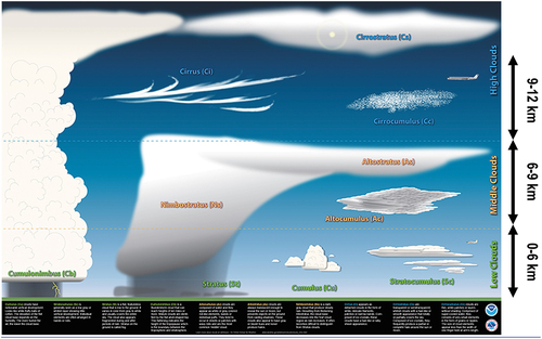
Acknowledged by the RS community, this observation (true-fact) implies that, since EO optical imagery are numerically affected by cloud cover, then the two causality-related problems of Cloud and Cloud-shadow detection (see Figure 6) ought to be accounted for as data quality layers, suitable for managing data uncertainty in EO optical imagery and image-derived information products, in agreement with an mDMI set of OP-Q²Is encompassing the popular FAIR guiding principles for scientific data (product and process) management (GO FAIR – International Support and Coordination Office, 2021; Wilkinson et al., 2016) (see Table 1) and the standard intergovernmental GEO- CEOS QA4EO Cal/Val requirements (refer to references listed in this Section above).

Figure 6. Adapted from (Baraldi & Tiede, 2018a, 2018b). Physical model, known a priori (available in addition to data), of the Sun-cloud-satellite geometry for arbitrary viewing and illumination conditions. Left: Actual 3D representation of the Sun/ cloud/ cloud–shadow geometry. Cloud height, h, is a typical unknown variable. Right: Apparent Sun/ cloud/ cloud–shadow geometry in a 2D soil projection, with a_g = h ⋅ tanφ_β, b_g = h ⋅ tanφ_μ.

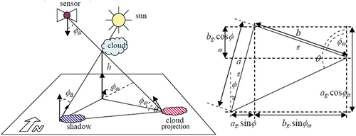
Figure 7. Adapted from (Swain & Davis, 1978). In the y-axis, reflectance values in physical range [0.0, 1.0] are represented as % values in range [0.0, 100.0], either ‘Top-of-atmosphere reflectance (TOARF) ⊇ Surface reflectance (SURF) ⊇ Surface albedo’ = Equation (8)(8) $\begin{array}{rl}& \text{lsquo}\mathrm{D}\mathrm{N}\mathrm{s}\ge 0\mathrm{a}\mathrm{t}\mathrm{E}\mathrm{O}\mathrm{L}\mathrm{e}\mathrm{v}\mathrm{e}\mathrm{l}0\supseteq \mathrm{T}\mathrm{O}\mathrm{A}\mathrm{R}\mathrm{F}\in \left[0.0,1.0\right]\mathrm{a}\mathrm{t}\mathrm{E}\mathrm{O}\mathrm{L}\mathrm{e}\mathrm{v}\mathrm{e}\mathrm{l}1\supseteq \mathrm{S}\mathrm{U}\mathrm{R}\mathrm{F}\in \left[0.0,1.0\right]\\ & \mathrm{a}\mathrm{t}\mathrm{E}\mathrm{O}\mathrm{L}\mathrm{e}\mathrm{v}\mathrm{e}\mathrm{l}2/\left(\mathrm{c}\mathrm{u}\mathrm{r}\mathrm{r}\mathrm{e}\mathrm{n}\mathrm{t}\right)\mathrm{A}\mathrm{R}\mathrm{D}\supseteq \mathrm{S}\mathrm{u}\mathrm{r}\mathrm{f}\mathrm{a}\mathrm{c}\mathrm{e}\mathrm{a}\mathrm{l}\mathrm{b}\mathrm{e}\mathrm{d}\mathrm{o}\in \left[0.0,1.0\right]\mathrm{a}\mathrm{t},\mathrm{s}\mathrm{a}\mathrm{y},\mathrm{E}\mathrm{O}\mathrm{L}\mathrm{e}\mathrm{v}\mathrm{e}\mathrm{l}3/\mathrm{n}\mathrm{e}\mathrm{x}\mathrm{t}\\ & \mathrm{g}\mathrm{e}\mathrm{n}\mathrm{e}\mathrm{r}\mathrm{a}\mathrm{t}\mathrm{i}\mathrm{o}\mathrm{n}\mathrm{A}\mathrm{R}\mathrm{D}\text{rsquo}& (8)\end{array}$(8) (refer to the farther Subsection 3.3.2), where surface albedo is included in the list of terrestrial Essential Climate Variables (ECVs) defined by the World Climate Organization (WCO), see Table 2. This graph shows the typical spectral response characteristics of “green (photosynthetically active) vegetation” in reflectance values (Liang, 2004; Swain & Davis, 1978), where chlorophyll absorption phenomena occur jointly with water content absorption phenomena, according to a convergence-of-evidence approach (Baraldi, 2017; Baraldi & Tiede, 2018a, 2018b; Matsuyama & Hwang, 1990). “In general, the total reflectance of a given object across the entire solar spectrum (also termed albedo) is strongly related to the physical condition of the relevant targets (shadowing effects, slope and aspect, particle size distribution, refraction index, etc.), whereas the spectral peaks or, vice versa, absorption valleys are more closely related to the chemical condition of the sensed target (material surface-specific absorption)” (Van der Meer & De Jong, 2011, p. 251). In the remote sensing (RS) literature and in the RS meta-science common practice, chlorophyll absorption phenomena are traditionally intercepted by so-called vegetation spectral indexes, such as the well-known two-band Normalized Difference Vegetation Index, NDVI (DLR – Deutsches Zentrum für Luft-und Raumfahrt e.V. and VEGA Technologies, 2011; ESA – European Space Agency, 2015; Jordan, 1969; Liang, 2004; Neduni & Sivakumar, 2019; Rouse, Haas, Scheel, & Deering, 1974; Sykas, 2020; Tucker, 1979), where NDVI ∈ [−1.0, 1.0] = f₁(Red, NIR) = f1(Red_0.65÷0.68, NIR_0.78÷0.90) = (NIR_0.78÷0.90 – Red_0.65÷0.68)/(NIR_0.78÷0.90 + Red_0.65÷0.68), which is monotonically increasing with the dimensionless Vegetation Ratio Index (VRI), where VRI ∈ (0, +∞) = NIR_0.78÷0.90/Red_0.65÷0.68 = (1. + NDVI)/(1. – NDVI) (Liang, 2004). Water content absorption phenomena in phenology are traditionally intercepted by so-called moisture or, vice versa, drought spectral indexes, such as the two-band Normalized Difference Moisture Index, NDMI (Liang, 2004; Neduni & Sivakumar, 2019; Sykas, 2020), equivalent to the Normalized Difference Water Index defined by Gao, NDWI_Gao (Gao, 1996), where NDMI ∈ [−1.0, 1.0] = NDWI_Gao = f₂(NIR, MIR1) = f₂(NIR_0.78÷0.90, MIR_1.57÷1.65) = (NIR_0.78÷0.90 – MIR_1.57÷1.65)/(NIR_0.78÷0.90 + MIR_1.57÷1.65), which is inversely related to the so-called Normalized Difference Bare Soil Index (NDBSI), NDBSI ∈ [−1.0, 1.0] = f3(NIR, MIR1) = (MIR_1.55÷1.75 – NIR_0.78÷0.90)/(MIR_1.55÷1.75 + NIR_0.78÷0.90) adopted in (Kang Lee, Dev Acharya, & Ha Lee, 2018; Roy, Miyatake, & Rikimaru, 2009), see Table 3. Popular two-band spectral indexes are conceptually equivalent to the angular coefficient/ slope/ 1^st-order derivative of a tangent to the spectral signature in one point (Baraldi, 2017, 2019a; Baraldi et al., 2010a, 2010b, 2018a, 2018b, 2006; Baraldi & Tiede, 2018a, 2018b; Liang, 2004). Three-band spectral indexes are conceptually equivalent to a 2^nd-order derivative as local measure of function concavity (Baraldi, 2017, 2019a; Baraldi et al., 2010a, 2010b, 2018a, 2018b, 2006; Baraldi & Tiede, 2018a, 2018b; Liang, 2004). Noteworthy, no combination of derivatives of any order can work as set of basis functions, capable of universal function approximation (Bishop, 1995; Cherkassky & Mulier, 1998). It means that if, in the fundamental feature engineering phase (Koehrsen, 2018) preliminary to feature (pattern) recognition (analysis, classification, understanding), any two-band or three-band scalar spectral index extraction occurs, then it always causes an irreversible loss in (lossy compression of) the multivariate shape and multivariate intensity information components of a spectral signature (Baraldi, 2017, 2019a; Baraldi et al., 2010a, 2010b, 2018a, 2018b, 2006; Baraldi & Tiede, 2018a, 2018b).

For example, in the RS common practice, “undetected cloudy pixels tremendously affect biophysical [variable]-retrieval methods [such as those involving EO data-derived estimation of biophysical ECVs defined by the WCO (Bojinski et al., 2014), see Table 2, pursued by the ESA Climate Change Initiative’s parallel projects (ESA – European Space Agency, 2017b, 2020a, 2020b) and by the GEO second implementation plan for years 2016–2025 of a GEOSS (GEO – Group on Earth Observations, 2015; Nativi et al., 2015, 2020; Santoro et al., 2017), see Figure 1]. Slight overmasking of potential cloudy pixels – conservative cloud masking – would be preferred in those cases in order to guarantee the quality of the final [value-adding information] product, while other applications, such as [land cover] classification [which is included, referred to as land cover, in the list of EO sensory data-derived ECVs defined by the WCO, see Table 2], are less sensitive to thin clouds and, thus, [do not require to overmask potential cloudy pixels]” (Gómez-Chova et al., 2007).

In more detail, the “Harmonization of Cloud Classes” task was assigned by ESA to the Copernicus data Quality Control team in order to, first, harmonize/ reconcile/ standardize existing Cloud cover definitions (to answer question: what to do in terms of product, see Figure 5) and, second, harmonize/ reconcile/ standardize existing Cloud and Cloud-shadow detection algorithms (to answer question: what to do, in terms of process, to accomplish the desired product), to be adopted as new product and process reference standard by the EO Copernicus Contributing Mission Entities, such as GAF AG responsible for the optical imaging payloads mounted onboard the Indian Remote sensing Satellite missions, Planet responsible for the EO spaceborne RapidEye constellation, etc. (ESA – European Space Agency, 2018). In the ESA common practice, the number and heterogeneity of EO Copernicus Contributing Mission Entities are monotonically increasing with time, which makes the “Harmonization of Cloud Classes” problem, together with its dual (complementary) causality-related problem of EO optical image-derived LC class detection in cloud-free Earth surface areas (see Figure 3), of increasing complexity and relevance for product and process interoperability, up to the third level of semantic interoperability (Durbha et al., 2008; Herold et al., 2009, 2006; Jansen et al., 2008).

Since the launch of the National Aeronautics and Space Administration (NASA) Earth Resources Technology Satellite (ERTS)-1 (Landsat-1) in 1972 (Rouse et al., 1974; Tucker, 1979), spaceborne/airborne EO optical imaging sensors have been ever increasing in both quantity and quality, operated by an increasing variety of either public or private EO big data providers (NASA – National Aeronautics and Space Administration, 2019; CEOS – Committee on Earth Observation Satellites, 2018; DLR – Deutsches Zentrum für Luft-und Raumfahrt e.V. and VEGA Technologies, 2011; Dwyer et al., 2018; ESA – European Space Agency, 2015; Gómez-Chova et al., 2007; Helder et al., 2018; Houborga & McCabe, 2018; OHB, 2016; USGS – U.S. Geological Survey, 2018a, 2018b, 2018c; Vermote & Saleous, 2007). Typically, EO imaging sensors are partitioned into “useful” categories by grouping their technical features, expressed in the techno-speak of spectrometry as part-of spectroscopy (Liang, 2004; Lillesand & Kiefer, 1979; Malenovsky et al., 2007; Swain & Davis, 1978; Van der Meer & De Jong, 2011). Spectroscopy is the branch of physics focused on the study of the interaction between matter and electromagnetic radiation. According to spectroscopy, absolute (quantitative) measurements of electromagnetic radiation reflected by a target surface convey significant information on surface properties, such as vegetation and soil properties of ecosystems on Earth (Liang, 2004; Lillesand & Kiefer, 1979; Swain & Davis, 1978; Van der Meer & De Jong, 2011), see Figure 7. Part-of spectroscopy is spectrometry (spectro-photometry), the measure of photons as a function of wavelength (Van der Meer & De Jong, 2011, p. 113). Spectrometry contributes to the RS meta-science with EO sensing devices, whose subset-of (special case) are EO imaging sensors whose outcome is an image, synonym for 2D gridded data set in a (2D) image-plane (refer to this Section above).

In the terminology of imaging spectrometry (Van der Meer & De Jong, 2011), the spectral resolution of an imaging sensor is typically described by the “full-width-half-maximum” (FWHM) of the instrument response to a monochromatic source, with central wavelength λ, synonym for sample point, located at the center of the FWHM (Liang, 2004; Lillesand & Kiefer, 1979; Malenovsky et al., 2007; Swain & Davis, 1978). The spectral extent, also named spectral range, is the difference between the minimum and maximum wavelengths, (λmax – λmin), in which measurements are made. Discrete spectral sampling is the parameter introduced to describe the number and position of the spectral channels. Spectral sampling interval is the spacing between sample points λs in the spectrum (Liang, 2004; Malenovsky et al., 2007), see Figure 8. In addition to spectral sampling and spectral resolution, fundamental EO imaging sensor specifications are spatial resolution, temporal resolution and swath width (Liang, 2004; Lillesand & Kiefer, 1979; Swain & Davis, 1978).

Figure 8. Adapted from (Malenovsky et al., 2007). Spectral resolution (“full-width-half-maximum”, FWHM), central wavelength λ, extent (λmax – λmin) and sampling interval of imaging spectroscopy data.

Based on their spectral resolution (see Figure 8), EO optical imaging sensors and their output imagery can be categorized as follows (Swain & Davis, 1978).

• Panchromatic (PAN), achromatic, one-band imaging spectrometry, whose typical spectral resolution, FWHM, belongs to range [0.35 μm, 0.75 μm] of visible (VIS) wavelengths, encompassing spectral channels visible blue (B, 0.45–0.50 μm), visible green (G, 0.50–0.57 μm) and visible red (R, 0.65–0.72 μm) (Lillesand & Kiefer, 1979), [61], see Figure 7. Because their FWHM is “large”, PAN sensors feature “high” sensitivity in collecting surface radiance; hence, their typical spatial resolution is “fine” or “very fine”, e.g. typically < 1 m in EO spaceborne PAN imaging sensors developed in recent years.

• Multi-spectral (MS) imaging spectrometry, featuring 2 to 9 spectral channels (Lillesand & Kiefer, 1979; Swain & Davis, 1978) of relatively large bandwidth, whose FWHM ranges among 70–400 nm (Liang, 2004, p. 272). It is also known as broadband spectrometry (Liang, 2004; Malenovsky et al., 2007; Van der Meer & De Jong, 2011), including Red-Green-Blue (RGB) cameras in either true- or false-colors. Started in the late 1960’s (Jordan, 1969; Kriegler, Malila, Nalepka, & Richardson, 1969), broadband spectrometry is increasingly popular since the launch of the NASA ERTS-1 (Landsat-1) in 1972 (Rouse et al., 1974; Tucker, 1979). Traditional spaceborne MS imaging sensors are the 5-band National Oceanic and Atmospheric Administration (NOAA) Advanced Very High Resolution Radiometer (AVHRR) sensor-series, the 7-band Landsat Thematic Mapper (TM)-sensor series, etc. (Liang, 2004).

• Super-spectral (SS) imaging spectrometry, featuring 10 to 20 spectral channels (Lillesand & Kiefer, 1979; Swain & Davis, 1978), where at least some channels are typically narrowband, whose FWHM ranges among 5–10 nm (Liang, 2004, p. 272). Developed since the early 2000s, popular EO spaceborne SS imaging sensors are the ESA 15-band ENVISAT Medium Resolution Imaging Spectrometer Instrument (MERIS), ESA 12-band Sentinel-2 Multi-Spectral Instrument (MSI) (DLR – Deutsches Zentrum für Luft-und Raumfahrt e.V. and VEGA Technologies, 2011; ESA – European Space Agency, 2015), ESA 11-band Sentinel-3 Sea and Land Surface Temperature Radiometer (SLSTR), DigitalGlobe 16-band WorldView-3 (DigitalGlobe, 2017), NOAA 16-band Geostationary Operational Environmental Satellites (GOES) Advanced Baseline Imager (ABI), etc.

• Hyper-spectral (HS) imaging spectrometry, featuring more than 20 spectral channels (Lillesand & Kiefer, 1979; Swain & Davis, 1978) of relatively narrow bandwidths, whose FWHM ranges among 5–10 nm (Liang, 2004, p. 272), also known as narrowband spectrometry (Liang, 2004; Malenovsky et al., 2007; Van der Meer & De Jong, 2011). HS imaging started from the mid-1980s with airborne imaging spectrometers, such as the Jet Propulsion Laboratory (JPL) 220-band Airborne Visible Near Infrared Imaging Spectrometer (AVIRIS), the ESA 285-band Airborne Prism Experiment (APEX), etc. Well-known spaceborne instances are the NASA 36-band Moderate Resolution Imaging Spectroradiometer (MODIS), ESA 21-band Sentinel-3 Ocean and Land Color Instrument (OLCI), ESA 62-band Project for OnBoard Autonomy (PROBA) Compact High Resolution Imaging Spectrometer (CHRIS), Cosine 49-band HyperScout-2 (Esposito et al., 2019b) suitable for small satellites from 500 Kg to 100 Kg, micro-satellites from 100 Kg to 10 Kg and nano-satellies from 10 Kg to 1 Kg (Satellite Applications Catapult, 2018), etc.

In terms of an mDMI set of OP-Q²Is to be jointly optimized (refer to this Section above), the ever-increasing spectral (color) data space dimensionality accomplished by EO imaging spectrometry in the last 60 years, while moving from MS to SS and HS imagery, becomes a matter of trade-offs. On the hand, it means increasing costs in computation time, data storage, run-time memory occupation and size of the training samples required by any inductive machine learning (ML)-from-data algorithm to cope with the well-known curse of (input) data dimensionality (Bishop, 1995; Cherkassky & Mulier, 1998). On the other hand, through a more detailed discrete sampling of the continuous electromagnetic spectrum (see Figures 7 and 8), SS and HS imaging sensors aim at improving sensitivity to vegetation and soil variables characterized by narrowband (local, in the spectral domain) colorimetric properties, occurring at fine spectral resolution, assuming that the SS/HS imaging sensor at hand features a spatial resolution fine enough to detect the target LC class-specific objects on the Earth surface.

In the RS literature, a typical rule of thumb in EO optical imaging sensor requirements specification is that spatial resolution should be ≤ (1/4) ÷ 1 times the spatial size of the real-world object of interest, to be detected on the Earth surface (Lillesand & Kiefer, 1979; Richter & Schläpfer, 2012; Swain & Davis, 1978).

When EO image-wide (summary) statistics are collected at large spatial extents, local non-stationary image statistics typically become indistinguishable (Egorov, Roy, Zhang, Hansen, and Kommareddy, 2018), in agreement with the central limit theorem (Kreyszig, 1979; Sheskin, 2000; Tabachnick & Fidell, 2014). For example, the Pearson linear cross-correlation (PLCC) coefficient (Kreyszig, 1979; Sheskin, 2000; Tabachnick & Fidell, 2014), belonging to range [−1.0, 1.0], typically scores (fuzzy) “high” (close to 1) when it is estimated image-wide from a pair of adjacent HS (narrow) channels selected within each of the four well-known physical model-based portions of the electromagnetic spectrum, namely, visible (VIS) ∈ (0.65–0.72 μm), Near-Infrared (NIR) ∈ (0.72–1.3 μm), Middle-Infrared (MIR) ∈ (1.3–3.0 μm) and Thermal-Infrared (TIR) ∈ (8.0–12.0 μm) (Van der Meer & De Jong, 2011) (see Figure 7), whereas PLCC values score (fuzzy) “(absolute) low” (close to 0) when the band pair is selected across the four spectral portions, see Figure 9. It means that overall (globally, image-wide, at large spatial extent) HS image redundancy (inter-band PLCC) is typically “high” within portions VIS, NIR, MIR and TIR of the electromagnetic spectrum, when local non-stationary image statistics, if any, are not taken into account at small spatial extent (because, at large spatial extent, the central limit theorem comes into play) (Kreyszig, 1979; Sheskin, 2000; Tabachnick & Fidell, 2014).

Figure 9. Adapted from (Van der Meer and De Jong, 2011). Inter-band Pearson’s linear cross-correlation (PLCC) coefficient, in range [−1.0, 1.0] (Kreyszig, 1979; Sheskin, 2000; Tabachnick & Fidell, 2014), for the main factors resulting from a principal component analysis and factor rotation for an agricultural data set acquired by the 220-band Jet Propulsion Laboratory (JPL) 220-band Airborne Visible Near Infrared Imaging Spectrometer (AVIRIS). Flevoland test site, July 5th 1991. It shows that, a global image-wide inter-band PLCC estimate, where typical local image non-stationarities are lost (Egorov, Roy, Zhang, Hansen, and Kommareddy, 2018) because averaged (wiped out), according to the central limit theorem (Kreyszig, 1979; Sheskin, 2000; Tabachnick & Fidell, 2014), scores (fuzzy) “high” (close to 1) within each of the three portions of the electromagnetic spectrum, namely, visible (VIS) ∈ [0.35 μm, 0.72 μm], Near-Infrared (NIR) ∈ [0.72 μm, 1.30 μm] and Middle-Infrared (MIR) ∈ [1.30 μm, 3.00 μm), see Figure 7.

The convergence of evidence stemming from Figures 7 and 9 reveals that, in the RS common practice, HS imagery should be considered feasible and more informative than traditional MS imagery if and only if the cognitive (interpretation) process of ‘AGI ⊃ CV ⊃ EO-IU’ of HS imagery is based on evidence stemming from local (rather than global) geospatial statistics collected at fine spectral resolution, to intercept geolocal variations/non-stationarities in HS properties of Earth surfaces at small spatial extents, assuming that the imaging sensor’s spatial and spectral resolutions are fine enough to detect subtle (narrowband) colorimetric properties of target real-world objects projected onto the (2D) image-plane (refer to this Section above).

This also means that, for improved computational efficiency, HS image analysis (interpretation, classification, understanding) should be conducted hierarchically, according to a Bayesian (stratified, class-conditional) approach to statistical data analysis (Bowers & Davis, 2012; Ghahramani, 2011; Hunt & Tyrrell, 2012; Lähteenlahti, 2021; Quinlan, 2012; Sarkar, 2018). First, suitable for image interpretation (classification) at large spatial extents and shallow semantics (at coarse semantic granularity), like at the first dichotomous level of the standard FAO 3-level 8-class LCCS-DP taxonomy (Ahlqvist, 2008; Di Gregorio, 2016; Di Gregorio & Jansen, 2000; Owers et al., 2021), consisting of the two dichotomous LC classes Vegetation and Not-vegetation (see Figure 3), few broadband spectral channels, required to be mutually uncorrelated, can be extracted as weighted sums of narrowbands. For example, four HS data-derived broadbands, one broadband located in the VIS portion of the electromagnetic spectrum, one in NIR, one in MIR and one in TIR (see Figure 7), would mimic the spectral resolution of the popular AVHRR imaging sensor series, regarded by NOAA (and by the present authors) as the best possible trade-off between dimensionality and informativeness of the MS data space, according to an image-wide inter-band PLCC minimization criterion, see Figure 9. Second, this 4-band AVHRR-like MS image can be interpreted at a 1^st hierarchical classification level featuring coarse semantic granularity, say, two-class Vegetation and Not-vegetation in agreement with a standard FAO LCCS-DP taxonomy, see Figure 3. Finally, at local spatial extents and finer semantics in the adopted hierarchical LC class taxonomy, e.g. to spectrally detect 2^nd-level LC class Oak trees stratified/ layered/ class-conditioned by the 1^st-level LC class Vegetation, narrowband HS imagery can be interpreted, at fine spectral detail, in agreement with a Bayesian (class-conditional, masked, stratified, driven-by-prior-knowledge) data analysis paradigm (refer to references listed in this Section above).

In recent years, the ever-increasing availability of multi-source EO large PAN, MS, SS and HS image databases, whose six Vs of volume, variety, veracity, velocity, volatility and value (Metternicht et al., 2020) must be successfully coped with to deliver operational, timely and comprehensive EO image-derived VAPS, has urged relevant portions of the RS meta-science community to promote the notion of Analysis Ready Data (ARD) (CEOS – Committee on Earth Observation Satellites, 2018; Dwyer et al., 2018; Helder et al., 2018; NASA – National Aeronautics and Space Administration, 2019; Qiu et al., 2019; USGS – U.S. Geological Survey, 2018a, 2018c). In agreement with commonsense knowledge and with the GEO-CEOS QA4EO Cal/Val requirements (refer to this Section above), quantitative/unequivocal big data analysis of scientific quality requires numerical variables to be better constrained, to become better behaved and better understood (Baraldi, 2009; Pacifici et al., 2014), than numerical variables typically employed in qualitative data analysis, either manual or semi-automatic, which is prone to bias, hard to reproduce and doesn’t scale to the huge amounts of sensory data available today. In this operational framework, the notion of ARD aims at enabling expert and non-expert end-users of space technology to access/retrieve EO big data ready for use in quantitative data analysis of scientific quality, without requiring laborious EO image pre-processing for geometric data enhancement, radiometric data enhancement and EO data QA, including Cloud and Cloud-shadow quality layers detection in EO optical imagery, preliminary to EO image processing (analysis, interpretation) by end-users.

For example, the popular Google Earth Engine Timelapse application (ESA – European Space Agency, 2021; Google Earth Engine, 2021) shows videos of multi-year time-series of spaceborne multi-sensor EO optical images of heterogeneous/non-harmonized radiometric quality, where no ARD policy for accomplishing multi-source multi-temporal EO data harmonization/ standardization/ interoperability is adopted. In practice, the Google Earth Engine Timelapse application is suitable for gaining a “wow” effect in qualitative human photointerpretation exclusively, equivalent to manmade works of art. Unfortunately, it is completely inadequate for quantitative big data analysis of scientific quality, which would require a (super) human-level ‘EO-IU ⊂ CV ⊂ AGI’ system in operational mode, capable of coping with the six Vs of big image databases (Metternicht et al., 2020), which does not exist yet (refer to this Section below).

In the ensemble of alternative EO optical image-derived Level 2/ARD product definitions and software implementations existing to date (NASA – National Aeronautics and Space Administration, 2019; ASI – Agenzia Spaziale Italiana, 2020; Bilal et al., 2019; CEOS – Committee on Earth Observation Satellites, 2018; DLR – Deutsches Zentrum für Luft-und Raumfahrt e.V. and VEGA Technologies, 2011; Dwyer et al., 2018; ESA – European Space Agency, 2015; Gómez-Chova et al., 2007; Helder et al., 2018; OHB, 2016; Qiu et al., 2019; USGS – U.S. Geological Survey, 2018a, 2018b, 2018c; Vermote & Saleous, 2007), Cloud and Cloud-shadow quality layers (strata, masks) are typically considered necessary to model data uncertainty (vice versa, veracity) in EO optical imagery, known that Cloud and Cloud-shadow detection in EO optical imagery consists of two causality-related data interpretation (understanding) problems in the multi-disciplinary domain of ‘EO-IU ⊂ CV ⊂ AGI ⊂ Cognitive science’ = Equation (2)(2) $\text{lsquo}\mathrm{C}\mathrm{o}\mathrm{g}\mathrm{n}\mathrm{i}\mathrm{t}\mathrm{i}\mathrm{v}\mathrm{e}\mathrm{s}\mathrm{c}\mathrm{i}\mathrm{e}\mathrm{n}\mathrm{c}\mathrm{e}\supset \mathrm{A}\mathrm{G}\mathrm{I}\supset \mathrm{C}\mathrm{V}\supset \mathrm{E}\mathrm{O}\text{-}\mathrm{I}\mathrm{U}\text{rsquo}$(2) , see Figure 6. In other words, Cloud and Cloud-shadow detection in EO optical imagery is an “AGI-complete” problem (Saba, 2020c; Wikipedia, 2021a), i.e. it is inherently ill-posed in the Hadamard sense (Hadamard, 1902) and non-deterministic polynomial (NP)-hard in computational complexity (Frintrop, 2011; Tsotsos, 1990), like any other ‘AGI ⊃ CV ⊃ EO-IU’ problem. It means that if Cloud and Cloud-shadow quality layers detection is accomplished successfully in multi-sensor EO optical imagery by an ‘EO-IU ⊂ CV’ system in operational mode (refer to this Section below), then any other ‘CV ⊃ EO-IU’ problem can be coped with successfully by the same ‘CV ⊃ EO-IU’ system solutions, investigated at the Marr five levels of system understanding (refer to the farther Subsection 3.2).

It is straightforward (intuitive, obvious), but not trivial to conclude that systematic generation of multi-source EO optical image-derived ARD products, where causality-related quality layers Cloud and Cloud-shadow (see Figure 6) are considered necessary to model EO optical image uncertainty (vice versa, veracity), is an EO image interpretation (understanding, classification) task, pertaining to the multi-disciplinary domain of cognitive science, centered on inherently ill-posed/ qualitative/ equivocal information-as-data-interpretation tasks. Intuitively, cognitive science focuses on how a sign/ symbol/ form (e.g. word in a language) or a sensory data sample is mapped onto (connected to, interpreted based on) a 7D (refer to this Section above) conceptual (mental) model of the physical real-world (see Figure 6) by an interpretant (Ball, 2021; Peirce, 1994; Perez, 2020, 2021; Salad, 2019; Santoro et al., 2021; Wikipedia, 2021e), in agreement with Peirce’s semiotics (refer to this Section below). Hence, ARD generation is regarded as a cognitive task, pertaining to the multi-disciplinary domain of cognitive science, where semantic relationship

(3) $\text{lsquo}\mathrm{A}\mathrm{R}\mathrm{D}\subset \mathrm{E}\mathrm{O}-\mathrm{I}\mathrm{U}\subset \mathrm{C}\mathrm{V}\subset \mathrm{A}\mathrm{G}\mathrm{I}\subset \mathrm{C}\mathrm{o}\mathrm{g}\mathrm{n}\mathrm{i}\mathrm{t}\mathrm{i}\mathrm{v}\mathrm{e}\mathrm{s}\mathrm{c}\mathrm{i}\mathrm{e}\mathrm{n}\mathrm{c}\mathrm{e}\text{rsquo}$(3)

holds as an extension of Equation (2)(2) $\text{lsquo}\mathrm{C}\mathrm{o}\mathrm{g}\mathrm{n}\mathrm{i}\mathrm{t}\mathrm{i}\mathrm{v}\mathrm{e}\mathrm{s}\mathrm{c}\mathrm{i}\mathrm{e}\mathrm{n}\mathrm{c}\mathrm{e}\supset \mathrm{A}\mathrm{G}\mathrm{I}\supset \mathrm{C}\mathrm{V}\supset \mathrm{E}\mathrm{O}\text{-}\mathrm{I}\mathrm{U}\text{rsquo}$(2) .

The potential impact of the cognitive problem of ‘ARD ⊂ EO-IU ⊂ CV ⊂ AGI’ = Equation (3)(3) $\text{lsquo}\mathrm{A}\mathrm{R}\mathrm{D}\subset \mathrm{E}\mathrm{O}-\mathrm{I}\mathrm{U}\subset \mathrm{C}\mathrm{V}\subset \mathrm{A}\mathrm{G}\mathrm{I}\subset \mathrm{C}\mathrm{o}\mathrm{g}\mathrm{n}\mathrm{i}\mathrm{t}\mathrm{i}\mathrm{v}\mathrm{e}\mathrm{s}\mathrm{c}\mathrm{i}\mathrm{e}\mathrm{n}\mathrm{c}\mathrm{e}\text{rsquo}$(3) on the RS community is highlighted by recalling here that the notion of ARD has been strictly coupled with the concept of EO (raster-based) data cube, proposed as innovative midstream EO technology by the RS community in recent years (Open Data Cube, 2020; Baumann, 2017; CEOS – Committee on Earth Observation Satellites, 2020; Giuliani et al., 2017, 2020; Lewis et al., 2017; Strobl et al., 2017). Prior to these developments, at the midstream segment EO images were organized according to a traditional file-based approach, similar to how people organize pictures acquired by their digital camera: individual files located in some directories on a hard drive. Compared to purely file-based approaches, an EO (raster-based) data cube is a new way of organizing EO big data, characterized by the aforementioned six Vs (Metternicht et al., 2020) to be coped with for augmenting data and/or information findability, accessibility and usability (Strobl et al., 2017). An EO big data cube is considered a multi-dimensional structure with at least one non-geospatial dimension, such as time. Although it can have any number of dimensions, it is referred to as “cube” (Strobl et al., 2017). In EO imagery, every pixel is associated with a unique position on the Earth surface, identified by 4D geospace-time coordinates and not by file and directory names. In EO (raster-based) big data cube management systems, a software translates the geographic position on a digital globe to the internal file structure, collects EO images and presents them in a way that is convenient, showing the pixels at their geographic position. Hence, it is possible to interact with an EO data cube by using geospatial and temporal coordinates instead of file names, because the EO (raster-based) data cube acts as a translation layer to the image files.

Synonym for EO (raster-based) big data cube whose sensory data belong to the 4D geospace-time physical world-domain, Digital (Twin) Earth is yet-another buzzword of increasing popularity (Craglia et al., 2012; Goodchild, 1999; Gore, 1999; Guo et al., 2020; ISDE – International Society for Digital Earth, 2012; Loekken, Le Saux, & Aparicio, 2020; Metternicht et al., 2020), stemming from Al Gore’s 1998 insight that “we need a Digital Earth, a multi-resolution, 3D representation of the planet, into which we can embed vast quantities of geo-referenced data” (Craglia et al., 2012; Gore, 1999; Loekken et al., 2020). A Digital (Twin) Earth is “an interactive digital replica of the entire planet that can facilitate a shared understanding of the multiple relationships between the physical and natural environments and society” (Guo et al., 2020). It is the pre-dating concept of Digital Twin of a complex system, defined as “a set of virtual information constructs that fully describes a potential or actual physical system from the micro atomic level to the macro geometrical level” (Grieves & Vickers, 2017), applied to planet Earth (Loekken et al., 2020).

Unfortunately, a community-agreed definition of EO big data cube does not exist yet, although several recommendations and implementations have been proposed (Open Data Cube, 2020; Baumann, 2017; CEOS – Committee on Earth Observation Satellites, 2020; Giuliani et al., 2017, 2020; Lewis et al., 2017; Strobl et al., 2017). A community-agreed definition of ARD, to be adopted as standard baseline in EO data cubes, does not exist either. As a consequence, in common practice, many EO (raster-based) data cube definitions and implementations do not require ARD to run and, vice versa, an ever-increasing ensemble of new (supposedly better) ARD definitions and/or ARD software implementations is proposed by the RS community, independently of a standardized/harmonized definition of EO big data cube management system. For example, about the current state of the Open Data Cube initiative, a quote of interest is: “the Open Data Cube initiative is an open source project born out of the need to better manage EO data. It provides the foundation of several international, regional to national scale data architecture solutions, such as Digital Earth Australia, Africa Regional Data Cube, and others (Giuliani et al., 2017, 2020; Lewis et al., 2017). The Data Cube works well with ARD, pre-processed, ready-to-use data made available by data providers. While providers work on making global ARD products available on the cloud, the Data Cube typically uses the U.S. Geological Survey collection 1 Landsat 8 for demonstrations. These data are not ARD and should not be used for scientific analysis. In 2019, it is expected ARD data will become easily available on the Cloud, and until then a user can simply add and index their own processed data. Any data available to a user can be installed on the user’s cube, including commercial, in situ, or derived products” (Open Data Cube, 2020; CEOS – Committee on Earth Observation Satellites, 2020).

Back to task “Harmonization of Cloud Classes” assigned by ESA to the Copernicus data Quality Control team, to augment the semantic/ontological level of interoperability/ harmonization/ standardization (Sheth, 2015) among multi-source EO sensory data-derived Level 1, Level 2 and ARD products delivered by an ever-increasing variety of public and private EO big data providers, where Cloud and Cloud-shadow quality layers, characterized by a causal relationship (see Figure 6), are required to manage EO optical image uncertainty (vice versa, veracity) (NASA – National Aeronautics and Space Administration, 2019; CEOS – Committee on Earth Observation Satellites, 2018; DLR – Deutsches Zentrum für Luft-und Raumfahrt e.V. and VEGA Technologies, 2011; Dwyer et al., 2018; ESA – European Space Agency, 2015; Gómez-Chova et al., 2007; Helder et al., 2018; Houborga & McCabe, 2018; OHB, 2016; USGS – U.S. Geological Survey, 2018a, 2018b, 2018c; Vermote & Saleous, 2007), the Copernicus data Quality Control team recommended for use the following Cloud versus Not-Cloud (Rest-of-the-world) taxonomy (thematic map legend) (ESA – European Space Agency, 2017a), as part-of a conceptual world model (refer to this Section above).

1. Haze (thin clouds) quality layer, where the Earth surface is visible through the cloud cover, at least in some portions of the electromagnetic spectrum, ranging from visible to thermal channels.

   1. Almost transparent haze, including thin cirrus/water-ice clouds (Borduas & Donahue, 2018), see Figure 5. “Ice clouds, also called cirrus clouds, which include cirrus, cirrostratus, and cirrocumulus, are made up of ice crystals” (Borduas & Donahue, 2018). Located in the upper troposphere (6–10 km) or lower stratosphere (10–16 km) (Borduas & Donahue, 2018; NIWA – National Institute of Water and Atmospheric Research, 2018; U.S. National Weather Service, 2019; UCAR – University Corporation for Atmospheric Research, Center for Science Education – SCIED, 2018). Worth mentioning, the troposphere is typically located between 0 and 10 km of height (Borduas & Donahue, 2018; NIWA – National Institute of Water and Atmospheric Research, 2018; U.S. National Weather Service, 2019; UCAR – University Corporation for Atmospheric Research, Center for Science Education – SCIED, 2018), known that the height of the top of the troposphere, called the tropopause (NIWA – National Institute of Water and Atmospheric Research, 2018), varies with latitude (it is lowest over the poles and highest at the equator) and by season (it is lower in winter and higher in summer) (UCAR – University Corporation for Atmospheric Research, Center for Science Education – SCIED, 2018). In more detail, the tropopause can be as high as 20 km near the equator and as low as 7 km over the poles in winter (NIWA – National Institute of Water and Atmospheric Research, 2018; UCAR – University Corporation for Atmospheric Research, Center for Science Education – SCIED, 2018). Given that, above the troposphere, the stratosphere is typically located between 10 and 30 km of height (Baraldi, 2017; Borduas & Donahue, 2018; NIWA – National Institute of Water and Atmospheric Research, 2018; U.S. National Weather Service, 2019; UCAR – University Corporation for Atmospheric Research, Center for Science Education – SCIED, 2018).

   2. Semi-transparent haze/clouds, including thin cirrus/water-ice clouds (Borduas & Donahue, 2018).

2. Cloud quality layer, including thick cirrus/water-ice clouds (Borduas & Donahue, 2018), see Figure 5.

3. Cloud-shadow quality layer, related to clouds by a cause-effect relationship. In this causal relationship, if a Cloud instance is detected and the sun and sensor’s azimuth and zenith angles are known as image acquisition metadata parameters, then the sole physical model-free parameter is the cloud height, see Figure 6.

4. Terrestrial Snow and Ice, to be discriminated from cirrus/water-ice clouds.

5. Clear (no-cloud). It encompasses Rest-of-the-world surface types, excluding Cloud, Cloud-shadow and terrestrial Snow. As such, this class (entity) of a conceptual world model is expected to include LC classes Bare soil, Vegetation, Water, etc. For example, these LC classes can be defined according to a standard LC class taxonomy, such as the increasingly popular fully-nested two-stage FAO LCCS, consisting of an 8-class 3-layer DP taxonomy followed by a per-class MHP taxonomy (Ahlqvist, 2008; Di Gregorio, 2016; Di Gregorio & Jansen, 2000; Owers et al., 2021), see Figure 3.

Based on commonsense knowledge (refer to this Section above), encompassing “thinking in counterfactuals” (Dandl & Molnar, 2021) (refer to this Section above), to accomplish any target one-class detection with high accuracy (for inclusion purposes), say, Cloud detection, the dual problem of non-target class detection with high accuracy (for exclusion purposes), say, Not-Cloud (Rest of the-world-domain of interest) detection, must be accomplished simultaneously (jointly) with high combined accuracy. For example, to accomplish pattern recognition tasks with high accuracy and high robustness to changes in sensory data, human beings typically adopt a convergence-of-evidence approach, where both pattern recognition evidence and pattern exclusion evidence are combined, for example, according to fuzzy logic criteria (Zadeh, 1965). In human reasoning (Newell & Simon, 1972), a convergence-of-evidence approach allows to infer typically strong conjectures from independent sources of evidence, even when input information sources are individually weak (Baraldi, 2017; Matsuyama & Hwang, 1990).

Moving from the technical note issued by the Copernicus data Quality Control team for use by ESA as reference work (ESA – European Space Agency, 2017a), the present methodological and survey paper aims at two main objectives.

1. About question “what to do?”: In the multi-disciplinary domain of cognitive science, where Equation (3)(3) $\text{lsquo}\mathrm{A}\mathrm{R}\mathrm{D}\subset \mathrm{E}\mathrm{O}-\mathrm{I}\mathrm{U}\subset \mathrm{C}\mathrm{V}\subset \mathrm{A}\mathrm{G}\mathrm{I}\subset \mathrm{C}\mathrm{o}\mathrm{g}\mathrm{n}\mathrm{i}\mathrm{t}\mathrm{i}\mathrm{v}\mathrm{e}\mathrm{s}\mathrm{c}\mathrm{i}\mathrm{e}\mathrm{n}\mathrm{c}\mathrm{e}\text{rsquo}$(3) = ‘ARD ⊂ EO-IU ⊂ CV ⊂ AGI ⊂ Cognitive science’ holds, enhance the aforementioned Cloud versus Not-Cloud (Rest-of-the-world) taxonomy, proposed in (ESA – European Space Agency, 2017a), to augment information coped with by a harmonized/standardized EO sensory data-derived Level 1 and Level 2/ARD product and process (NASA – National Aeronautics and Space Administration, 2019; CEOS – Committee on Earth Observation Satellites, 2018; DLR – Deutsches Zentrum für Luft-und Raumfahrt e.V. and VEGA Technologies, 2011; Dwyer et al., 2018; ESA – European Space Agency, 2015; Gómez-Chova et al., 2007; Helder et al., 2018; Houborga & McCabe, 2018; OHB, 2016; USGS – U.S. Geological Survey, 2018a, 2018b, 2018c; Vermote & Saleous, 2007), featuring semantic/ontological interoperability (refer to this Section above) across multiple EO optical imaging sensors, see Figure 2.

   For example, in agreement with commonsense knowledge (refer to references listed in this Section above) and with traditional EO image classification system design and implementation requirements (refer to references listed in this Section above), to detect any finite set of target classes, say, the target single class Cloud, equivalent to one ARD quality layer (NASA – National Aeronautics and Space Administration, 2019; CEOS – Committee on Earth Observation Satellites, 2018; DLR – Deutsches Zentrum für Luft-und Raumfahrt e.V. and VEGA Technologies, 2011; Dwyer et al., 2018; ESA – European Space Agency, 2015; Helder et al., 2018; Houborga & McCabe, 2018; OHB, 2016; USGS – U.S. Geological Survey, 2018a, 2018b, 2018c; Vermote & Saleous, 2007), the explicit modeling of the dual (complementary) output class “Unknown” (“Others”, “Outliers”, “Rest of the world-domain of interest”) is considered mandatory, to cope with (semantic) uncertainty (refer to this Section above).

   Semantic uncertainty is congenital in information-as-data-interpretation tasks (Capurro & Hjørland, 2003), such as data classification problems, synonym for mapping ever-varying numerical or categorical subsymbolic variables (sensations) into symbolic (categorical and semantic) classes (percepts) belonging to a stable/hard-to-vary, but plastic conceptual world ontology (refer to this Section above). In short, the notion of information-as-data-interpretation is inherently qualitative/ equivocal (Capurro & Hjørland, 2003)/ ill-posed in the Hadamard sense (Baraldi, 2017; Baraldi & Tiede, 2018a, 2018b; Hadamard, 1902).

   By definition, an inherently ill-posed problem in the Hadamard sense admits (Baraldi, 2017; Baraldi & Tiede, 2018a, 2018b; Hadamard, 1902):

   • no solution,

   • multiple solutions or

   • if the solution exists, the solution’s behavior changes continuously with the initial conditions.

   In agreement with philosophical hermeneutics (Capurro & Hjørland, 2003; Dreyfus, 1965, 1991, 1992; Fjelland, 2020), the notion of qualitative/ equivocal/ inherently ill-posed information-as-data-interpretation, to be coped with by cognitive science encompassing AGI (see Equation (3)(3) $\text{lsquo}\mathrm{A}\mathrm{R}\mathrm{D}\subset \mathrm{E}\mathrm{O}-\mathrm{I}\mathrm{U}\subset \mathrm{C}\mathrm{V}\subset \mathrm{A}\mathrm{G}\mathrm{I}\subset \mathrm{C}\mathrm{o}\mathrm{g}\mathrm{n}\mathrm{i}\mathrm{t}\mathrm{i}\mathrm{v}\mathrm{e}\mathrm{s}\mathrm{c}\mathrm{i}\mathrm{e}\mathrm{n}\mathrm{c}\mathrm{e}\text{rsquo}$(3) ), is dual (complementary, not alternative) to the notion of quantitative/unequivocal information as-thing (Capurro & Hjørland, 2003), typical of the Shannon data communication/transmission theory (Baraldi, 2017; Baraldi et al., 2018a, 2018b; Baraldi & Tiede, 2018a, 2018b; Capurro & Hjørland, 2003; Santoro et al., 2021; Shannon, 1948) (for more details on the two co-existing complementary not-alternative notions of quantitative/unequivocal information-as-thing and qualitative/equivocal information-as-data-interpretation, refer to the farther Subsection 3.3.3).

   The conclusion is that, to answer question “what to do?”, new harmonized/standardized EO sensory image-derived Level 1, Level 2/ARD product definitions and software implementations, capable of semantic/ontological interoperability over multiple EO optical imaging sensors, must be accomplished, in combination with (jointly with) a new harmonized/standardized definition and implementation of an EO big data cube management system as “horizontal” (enabling) midstream technology in the value chain required by a new notion of Space Economy 4.0, envisioned in 2017 by Mazzucato and Robinson in their original work for ESA (Mazzucato & Robinson, 2017), see Figure 10.

   In a new notion of Space Economy 4.0 (Mazzucato & Robinson, 2017), first-stage “horizontal” (enabling) capacity building, coping with background conditions necessary to specialization, is preliminary to second-stage “vertical” (deep and narrow) specialization policies, suitable for coping with a potentially huge worldwide market of institutional and private end-users of space technology, see Figure 10.

   Not surprisingly, the aforementioned notion of new Space Economy 4.0 (Mazzucato & Robinson, 2017) (see Figure 10) is in line with the intuitive concept of commonsense knowledge (refer to this Section above), regarded herein as “horizontal” general-purpose knowledge baseline, equivalent to a necessary-but-not-sufficient precondition of any “vertical” (deep and narrow) user- and application domain-specific mental (conceptual) model (ontology) of the 4D geospace-time physical world (refer to this Section above).

   In line with the FAIR criteria for scientific data (product and process) management (GO FAIR – International Support and Coordination Office, 2021; Wilkinson et al., 2016) (see Table 1) and with the GEO-CEOS QA4EO Cal/Val requirements (refer to this Section above), an innovative semantics-enabled EO big data cube management system at the midstream segment, such as AGI4DIAS = Equation (1)(1) $\begin{array}{rl}& \text{lsquo}\mathrm{A}\mathrm{G}\mathrm{I}\text{-}\mathrm{e}\mathrm{n}\mathrm{a}\mathrm{b}\mathrm{l}\mathrm{e}\mathrm{d}\mathrm{D}\mathrm{I}\mathrm{A}\mathrm{S}=\mathrm{A}\mathrm{G}\mathrm{I}4\mathrm{D}\mathrm{I}\mathrm{A}\mathrm{S}=\mathrm{S}\mathrm{e}\mathrm{m}\mathrm{a}\mathrm{n}\mathrm{t}\mathrm{i}\mathrm{c}\mathrm{s}\text{-}\mathrm{e}\mathrm{n}\mathrm{a}\mathrm{b}\mathrm{l}\mathrm{e}\mathrm{d}\mathrm{D}\mathrm{I}\mathrm{A}\mathrm{S}2.0\\ & (\mathrm{D}\mathrm{I}\mathrm{A}\mathrm{S}{2}^{\mathrm{n}\mathrm{d}}\mathrm{g}\mathrm{e}\mathrm{n}\mathrm{e}\mathrm{r}\mathrm{a}\mathrm{t}\mathrm{i}\mathrm{o}\mathrm{n})=\mathrm{D}\mathrm{I}\mathrm{A}\mathrm{S}2.0=\mathrm{A}\mathrm{G}\mathrm{I}+\mathrm{D}\mathrm{I}\mathrm{A}\mathrm{S}1.0+\mathrm{S}\mathrm{C}\mathrm{B}\mathrm{I}\mathrm{R}+\mathrm{S}\mathrm{E}\mathrm{I}\mathrm{K}\mathrm{D}\text{rsquo}\end{array}$(1) , is expected to boost the downstream segment in developing an ever-increasing ensemble of VAPS in operational mode, suitable for use by a worldwide market of institutional and private end-users of space technology, expected to cope with grand societal challenges, such as the United Nations (UN) Sustainable Development Goals (SDGs) from year 2015 to 2030 at regional to global spatial extents (UN – United Nations, Department of Economic and Social Affairs, 2021), in a new era of Space Economy 4.0 (Mazzucato & Robinson, 2017), see Figure 10.

2. About question “how to do it?”: Overcome the technical vagueness of document (ESA – European Space Agency, 2017a), with special regard to “Section 4.2 – (Existing) Cloud classification (algorithms)” and “Appendix I – Suggested methods for Cloud detection”, by selecting suitable ‘CV ⊃ EO-IU ⊃ ARD’ system design(s), algorithm(s) and implementation(s) solutions, whenever possible, from the existing literature, to benefit from their technology readiness level (TRL) (Wikipedia, 2016), based on quantitative quality criteria, formalized as an mDMI set of OP-Q²Is to be community-agreed upon before multi-objective optimization, in agreement with the Pareto formal analysis of multi-objective optimization problems (refer to this Section above).

To accomplish these two working objectives while coping with the six Vs of volume, variety, veracity, velocity, volatility and value that characterize EO large image database analysis (Metternicht et al., 2020), the present methodological and survey paper adopts the Marr five levels of understanding (levels of abstraction) of an information processing system (Baraldi, 2017; Baraldi et al., 2018a, 2018b; Baraldi & Tiede, 2018a, 2018b; Marr, 1982; Quinlan, 2012; Sonka et al., 1994) to promote a “universal” ‘ARD ⊂ EO-IU ⊂ CV ⊂ AGI’ system in operational mode (Baraldi, 2017; Baraldi & Tiede, 2018a, 2018b), capable of identifying automatically (without human-machine interaction) and in near real-time (featuring polynomial computational complexity, such as linear complexity with image size) semantic classes {Cloud, Cloud-shadow, Rest-of-the-world = LC classes, Unknown} in multi-sensor single-date EO optical imagery, either PAN, MS, SS or HS (refer to this Section above), as precondition to interoperability of a new semantics-enriched ARD product-pair and process reference standard. An innovative multi-sensor EO optical image-derived semantics-enriched ARD co-product pair consists of:

1. A sensory image-derived numerical variable co-product, whose DNs in the (2D) image-plane feature “high” radiometric quality, in compliance with the GEO-CEOSS QA4EO Cal requirements. Specifically, pixels of a radiometrically calibrated EO optical image are provided with a physical meaning, a physical unit of radiometric measure and a physical range of change, starting from TOARF values in the physical range of change [0.0, 1.0] (Baraldi, 2009; Baraldi et al., 2014; DigitalGlobe, 2017; Helder et al., 2018) (see Figure 7), to be corrected from:

   • Atmospheric effects (NASA – National Aeronautics and Space Administration, 2019; ASI – Agenzia Spaziale Italiana, 2020; Chavez, 1988; DLR – Deutsches Zentrum für Luft-und Raumfahrt e.V. and VEGA Technologies, 2011; Dwyer et al., 2018; ESA – European Space Agency, 2015; Fuqin et al., 2012; Giuliani et al., 2020; Hagolle, Huc, Desjardins, Auer, & Richter, 2017; Helder et al., 2018; Houborga & McCabe, 2018; Liang, 2004; Lillesand & Kiefer, 1979; Main-Knorn, Louis, Hagolle, Müller-Wilm, & Alonso, 2018; Maxar, 2021; Pacifici, 2016; Pacifici et al., 2014; Planet, 2019; Richter & Schläpfer, 2012; Swain & Davis, 1978; USGS – U.S. Geological Survey, 2018a, 2018b, 2018c; Vermote & Saleous, 2007), and

   • Topographic effects (Baraldi, Gironda, & Simonetti, 2010; Bishop & Colby, 2002; Bishop, Shroder, & Colby, 2003; DLR – Deutsches Zentrum für Luft-und Raumfahrt e.V. and VEGA Technologies, 2011; ESA – European Space Agency, 2015; Riaño, Chuvieco, Salas, & Aguado, 2003; Richter & Schläpfer, 2012; Zhaoning, Guorui, Schaepman, & Zhao, 2020), and

   • Adjacency effects (DLR – Deutsches Zentrum für Luft-und Raumfahrt e.V. and VEGA Technologies, 2011; ESA – European Space Agency, 2015; Liang, 2004; Lilles and & Kiefer, 1979; Swain & Davis, 1978),

   into surface reflectance (SURF) values ∈ [0.0, 1.0], to be corrected from bidirectional reflectance distribution function (BRDF) effects into surface albedo values ∈ [0.0, 1.0] (Bilal et al., 2019; EC, 2020; Egorov, Roy, Zhang, Hansen, and Kommareddy, 2018; Franch et al., 2019; Fuqin et al., 2012; Malenovsky et al., 2007; Schaepman-Strub et al., 2006; Qiu et al., 2019; Shuai et al., 2020).

   Noteworthy, surface albedo is included (referred to as albedo) in the list of terrestrial ECVs defined by the WCO (see Table 2), which complies with requirements of the GEO second implementation plan for years 2016–2025 of a new GEOSS, regarded as expert EO data-derived information and knowledge system (GEO – Group on Earth Observations, 2015; Nativi et al., 2015, 2020; Santoro et al., 2017), see Figure 1.

   This “high-quality” radiometrically calibrated EO optical image co-product is systematically overlapped (stacked) with (Baraldi & Tiede, 2018a, 2018b):

2. A sensory image-derived symbolic (categorical and semantic) co-product, namely, a Scene Classification Map (SCM), whose thematic map legend (taxonomy) includes quality layers Cloud and Cloud-shadow, which improves and generalizes the existing well-known ESA EO Sentinel-2 imaging sensor-specific Level 2 SCM co-product, systematically delivered as output semantic co-product by the ESA Sentinel-2 (atmospheric, adjacency and topographic) Correction Prototype Processor (Sen2Cor), developed and run by ESA or distributed by ESA free-of-cost to be run on the user side (DLR – Deutsches Zentrum für Luft-und Raumfahrt e.V. and VEGA Technologies, 2011; ESA – European Space Agency, 2015).

   To date, in addition to quality layer Cloud and, eventually, quality layer Cloud-shadow, which is not always pursued, e.g. refer to (OHB, 2016), no SCM is generated as output co-product by any other existing EO optical image-derived Level 2/ARD product definition and/or software implementation, although LC classes are EO image-derived for Level 2/ARD internal use, to accomplish EO image masking/stratification strategies preliminary to EO data radiometric correction (NASA – National Aeronautics and Space Administration, 2019; CEOS – Committee on Earth Observation Satellites, 2018; Dwyer et al., 2018; Gómez-Chova et al., 2007; Helder et al., 2018; Houborga & McCabe, 2018; OHB, 2016; Tiede, Sudmanns, Augustin, & Baraldi, 2020; USGS – U.S. Geological Survey, 2018a, 2018b, 2018c; Vermote & Saleous, 2007) (refer to Figures 35 and Figures 36 below in this text).

   In agreement with Bayesian inference, synonym for stratified/ masked/ class-conditional/ driven-by-prior-knowledge data analysis (Bowers & Davis, 2012; Ghahramani, 2011; Hunt & Tyrrell, 2012; Lähteenlahti, 2021; Quinlan, 2012; Sarkar, 2018) as viable alternative to unconditional/driven-without-prior-knowledge data analysis, an SCM is no optional by-product, but a mandatory information product required as input layer to make better conditioned for numerical solution an inherently ill-posed problem of EO optical image radiometric correction. For example, it is well known that “classification is a prerequisite for the subsequent land cover-specific BRDF correction” (Malenovsky et al., 2007), when SURF values are corrected into surface albedo values (Bilal et al., 2019; EC, 2020; Egorov, Roy, Zhang, Hansen, and Kommareddy, 2018; Franch et al., 2019; Fuqin et al., 2012; Malenovsky et al., 2007; Qiu et al., 2019; Schaepman-Strub et al., 2006; Shuai et al., 2020).

   Noteworthy, an SCM is included (referred to as land cover) in the list of terrestrial ECVs defined by the WCO (see Table 2), which complies with requirements of the GEO second implementation plan for years 2016–2025 of a new GEOSS, regarded as expert EO data-derived information and knowledge system (GEO – Group on Earth Observations, 2015; Nativi et al., 2015, 2020; Santoro et al., 2017), see Figure 1.

   According to Owers et al. (2021), “[existing ARD do] not provide the information required by national agencies tasked with coordinating implementation of [the UN] SDGs. Instead, [national agencies] require standardised and informative end user products derived from ARD to track progress towards agreed targets. [Standardised and informative products required by end users include] land cover and its change over time, that contribute to the mapping and reporting on 14 of the 17 SDGs (GEO – Group on Earth Observations, 2020; Kavvada et al., 2020; Poussin et al., 2021). However, many nations lack access to an operational, standardised land cover product.”

Selected from the RS literature (Baraldi, 2017; Baraldi & Boschetti, 2012a, 2012b; Baraldi et al., 2014, 2018a, 2018b; Baraldi & Tiede, 2018a, 2018b), the following definition is adopted herein.

An information processing system, such as an ‘AGI ⊃ CV ⊃ EO-IU ⊃ ARD’ system, is considered in operational mode if and only if it scores (fuzzy) “high” in each Q²I belonging to an mDMI set of OP-Q²Is, to be community-agreed upon (Baraldi, 2017; Baraldi & Boschetti, 2012a, 2012b; Baraldi et al., 2014, 2018a, 2018b; Baraldi & Tiede, 2018a, 2018b). According to the Pareto formal analysis of multi-objective optimization problems, optimization of an mDMI set of OP-Q²Is is an inherently ill-posed problem in the Hadamard sense (Hadamard, 1902) (refer to this Section above), where many Pareto optimal solutions lying on the Pareto efficient frontier can be considered equally good (Boschetti et al., 2004). Any ‘AGI ⊃ CV ⊃ EO-IU ⊃ ARD’ system solution lying on the Pareto efficient frontier can be considered in operational mode, which means it is eligible for success in dealing with the six Vs of volume, variety, veracity, velocity, volatility and value featured by multi-sensor EO big data acquired in the 4D geospace-time physical-world domain (Metternicht et al., 2020).

The aforementioned definition of a data and information processing system in operational mode is neither obvious nor trivial. Actually, it is in contrast with a large portion of the RS literature, including the Copernicus data Quality Control reference document (ESA – European Space Agency, 2017a), where the sole EO data mapping (e.g. classification) accuracy is typically adopted as “universal” scalar Q²I, in spite of the fact that, in general, no “universal” scalar Q²I exists, due to the non-injective property of Q²Is of complex phenomena (for more details on the non-injectivity of Q²Is, refer to the farther Subsection 3.1).

To cope with the cognitive task of systematic ARD generation, formalized as Equation (3)(3) $\text{lsquo}\mathrm{A}\mathrm{R}\mathrm{D}\subset \mathrm{E}\mathrm{O}-\mathrm{I}\mathrm{U}\subset \mathrm{C}\mathrm{V}\subset \mathrm{A}\mathrm{G}\mathrm{I}\subset \mathrm{C}\mathrm{o}\mathrm{g}\mathrm{n}\mathrm{i}\mathrm{t}\mathrm{i}\mathrm{v}\mathrm{e}\mathrm{s}\mathrm{c}\mathrm{i}\mathrm{e}\mathrm{n}\mathrm{c}\mathrm{e}\text{rsquo}$(3) = ‘ARD ⊂ EO-IU ⊂ CV ⊂ AGI ⊂ Cognitive science’, Figure 11 provides an original graphical representation of postulates adopted herein as working hypotheses in the multi-disciplinary domain of cognitive science (refer to references listed in this Section above).

Figure 10. In a new notion of Space Economy 4.0, envisioned by Mazzucato and Robinson in 2017 in their original work for the European Space Agency (ESA) (Mazzucato & Robinson, 2017), first-stage “horizontal” (enabling) capacity building, coping with background conditions necessary to specialization, is preliminary to second-stage “vertical” (deep and narrow) specialization policies, suitable for coping with a potentially huge worldwide market of institutional and private end-users of space technology. Definitions adopted herein, in agreement with the new notion of Space Economy 4.0 proposed by Mazzucato and Robinson (Mazzucato & Robinson, 2017), are: Space segment, Upstream segment for «mission control» = Ground segment for «mission control», Ground segment for «user support» = Midstream segment infrastructures and services, Downstream segment = Downstream utility of space technology (Mazzucato & Robinson, 2017, pp. 6, 57), capable of transforming quantitative (unequivocal) Earth observation (EO) big sensory data into sensory data-derived value-adding information products and services (VAPS), suitable for use by a potentially huge worldwide market of institutional and private end-users of space technology. Artificial General Intelligence (AGI) for EO (AGI4EO) technologies should be applied as early as possible in the “seamless innovation chain” required by a new notion of Space Economy 4.0, starting from AGI for space segment (AGI4Space) applications, which include the notion of future intelligent EO satellites, provided with AGI onboard (EOportal, 2020; ESA – European Space Agency, 2019; Esposito et al., 2019a, 2019b; GISCafe News, 2018; Zhou, 2001), and AGI for Data and Information Access Services (AGI4DIAS) at the midstream segment (see Figure 2), such as systematic generation of multi-sensor Analysis Ready Data (ARD) and information products, eligible for direct use in analysis at the downstream segment, without requiring laborious data pre-processing (Baraldi & Tiede, 2018a, 2018b; CEOS – Committee on Earth Observation Satellites, 2018; Dwyer et al., 2018; Helder et al., 2018; NASA – National Aeronautics and Space Administration, 2019; Qiu et al., 2019; USGS – U.S. Geological Survey, 2018a, 2018c).

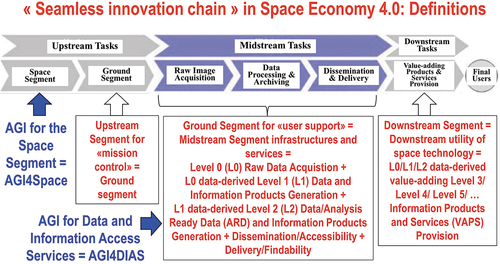
Figure 11. (a) Adapted from (Baraldi, 2017; Baraldi & Tiede, 2018a, 2018b), this original graph postulates that, within the multi-disciplinary cognitive science domain (Ball, 2021; Capra & Luisi, 2014; Hassabis et al., 2017; Hoffman, 2008, 2014; Langley, 2012; Miller, 2003; Mindfire Foundation, 2018; Mitchell, 2019; Parisi, 1991; Santoro et al., 2021; Serra & Zanarini, 1990; Varela et al., 1991; Wikipedia, 2019), encompassing disciplines like philosophy (Capurro & Hjørland, 2003; Dreyfus, 1965, 1991, 1992; Fjelland, 2020), semiotics (Ball, 2021; Peirce, 1994; Perez, 2020, 2021; Salad, 2019; Santoro et al., 2021; Wikipedia, 2021e), linguistics (Ball, 2021; Berlin & Kay, 1969; Firth, 1962; Rescorla, 2019; Saba, 2020a, 2020c), anthropology (Harari, 2011, 2017; Wikipedia, 2019), neuroscience (Barrett, 2017; Buonomano, 2018; Cepelewicz, 2021; Hathaway, 2021; Hawkins, 2021; Hawkins, Ahmad, and Cui, 2017; Kaufman, Churchland, Ryu, and Shenoy, 2014; Kosslyn, 1994; Libby & Buschman, 2021; Mason & Kandel, 1991; Salinas, 2021b; Slotnick et al., 2005; Zador, 2019), focusing on the study of the brain machinery in the mind-brain problem (Hassabis et al., 2017; Hoffman, 2008; Serra & Zanarini, 1990; Westphal, 2016), computational neuroscience (Beniaguev et al., 2021; DiCarlo, 2017; Gidon et al., 2020; Heitger et al., 1992; Pessoa, 1996; Rodrigues & Du Buf, 2009), psychophysics (Benavente et al., 2008; Bowers & Davis, 2012; Griffin, 2006; Lähteenlahti, 2021; Mermillod et al., 2013; Parraga et al., 2009; Vecera & Farah, 1997), psychology (APS – Association for Psychological Science, 2008; Hehe, 2021) computer science, formal logic (Laurini & Thompson, 1992; Sowa, 2000), mathematics, physics, statistics and (the meta-science of) engineering (Langley, 2012; Santoro et al., 2021; Wikipedia, 2019), semantic relationship ‘Human vision → Computer Vision (CV) ⊃ Earth observation (EO) image understanding (EO-IU)’ = Equation (4)(4) $\begin{array}{rl}& \text{lsquo}(Inductive/bottom\text{-}up/statisticalmodel\text{-}based)DL\text{-}from\text{-}data\subset \\ & (Inductive/bottom\text{-}up/statisticalmodel\text{-}based)ML\text{-}from\text{-}data\\ & \to AGI\supset CV\leftarrow Humanvision\text{rsquo}\end{array}$(4) holds true, where symbol ‘→’ denotes semantic relationship part-of (without inheritance) pointing from the supplier to the client, not to be confused with relationship subset-of, ‘⊃’, meaning specialization with inheritance from the superset (at left) to the subset, in agreement with symbols adopted by the standard Unified Modeling Language (UML) for graphical modeling of object-oriented software (Fowler, 2003). The working hypothesis ‘Human vision → CV ⊃ EO-IU’ = Equation (4)(4) $\begin{array}{rl}& \text{lsquo}(Inductive/bottom\text{-}up/statisticalmodel\text{-}based)DL\text{-}from\text{-}data\subset \\ & (Inductive/bottom\text{-}up/statisticalmodel\text{-}based)ML\text{-}from\text{-}data\\ & \to AGI\supset CV\leftarrow Humanvision\text{rsquo}\end{array}$(4) means that human vision is expected to work as lower bound of CV, i.e. a CV system is required to include as part-of a computational model of human vision (Baraldi, 2017; Baraldi et al., 2018a, 2018b; Baraldi & Tiede, 2018a, 2018b; Iqbal & Aggarwal, 2001), consistent with human visual perception, in agreement with a reverse engineering approach to CV (Baraldi, 2017; Bharath & Petrou, 2008; DiCarlo, 2017). In practice, to become better conditioned for numerical solution (Baraldi, 2017; Baraldi et al., 2018a, 2018b; Baraldi & Tiede, 2018a, 2018b; Bishop, 1995; Cherkassky & Mulier, 1998; Dubey, Agrawal, Pathak, Griffiths, & Efros, 2018), an inherently ill-posed CV system is required to comply with human visual perception phenomena in the multi-disciplinary domain of cognitive science. (b) In this original graph, the inherently vague/equivocal notion of Artificial Intelligence is disambiguated into the two concepts of Artificial General Intelligence (AGI) and Artificial Narrow Intelligence (ANI), which are better constrained to be better understood (Bills, 2020; Chollet, 2019; Dreyfus, 1965, 1991, 1992; EC – European Commission, 2019; Fjelland, 2020; Hassabis et al., 2017; Ideami, 2021; Jajal, 2018; Mindfire Foundation, 2018; Practical AI, 2020; Santoro et al., 2021; Sweeney, 2018a; Wolski, 2020a, 2020b). This graph postulates that semantic relationship ‘EO-IU ⊂ CV ⊂ Artificial General Intelligence (AGI) ← Artificial Narrow Intelligence (ANI) ← (Inductive/ bottom-up/ statistical model-based) Machine Learning-from-data (ML) ⊃ (Inductive/ bottom-up/ statistical model-based) Deep Learning-from-data (DL)’ = ‘EO-IU ⊂ CV ⊂ AGI ← ANI ← ML ⊃ DL’ = Equation (5)(5) $\text{lsquo}\mathrm{A}\mathrm{R}\mathrm{D}\subset \mathrm{E}\mathrm{O}\text{-}\mathrm{I}\mathrm{U}\subset \mathrm{C}\mathrm{V}\subset \mathrm{A}\mathrm{G}\mathrm{I}\leftarrow \mathrm{A}\mathrm{N}\mathrm{I}\leftarrow \mathrm{M}\mathrm{L}\supset \mathrm{D}\mathrm{L}\supset \mathrm{D}\mathrm{e}\mathrm{e}\mathrm{p}\mathrm{C}\mathrm{o}\mathrm{n}\mathrm{v}\mathrm{o}\mathrm{l}\mathrm{u}\mathrm{t}\mathrm{i}\mathrm{o}\mathrm{n}\mathrm{a}\mathrm{l}\mathrm{N}\mathrm{e}\mathrm{u}\mathrm{r}\mathrm{a}\mathrm{l}\mathrm{N}\mathrm{e}\mathrm{t}\mathrm{w}\mathrm{o}\mathrm{r}\mathrm{k}\left(\mathrm{D}\mathrm{C}\mathrm{N}\mathrm{N}\right)\text{rsquo}$(5) holds, where ANI is formulated as ‘ANI = [DL ⊂ ML logical-OR Traditional deductive Artificial Intelligence (static expert systems, non-adaptive to data, often referred to as Good Old-Fashioned Artificial Intelligence, GOFAI (Dreyfus, 1965, 1991, 1992; Santoro et al., 2021)]’ = Equation (6)(6) $x0026;\text{ANI=}[\text{DCNN}\subset \text{DL}\subset \text{ML}\text{logical0OR}\text{Traditional}\text{deductive}ArtificialIntelligencex0026;(\text{static}\text{expert}\text{systems},\text{non0adaptive}\text{to}\text{data},\text{also}\text{known}\text{as}\text{Good}\text{Old0Fashioned}x0026;ArtificialIntelligence,\text{GOFAI}]$(6) , in agreement with the entity-relationship model shown in (a). (c) In recent years, an increasingly popular thesis is that semantic relationship ‘A(G/N)I ⊃ ML ⊃ DL’ = Equation (7)(7) $\text{lsquo}\mathrm{A}(\mathrm{G}/\mathrm{N})\mathrm{I}\supset \mathrm{M}\mathrm{L}\supset \mathrm{D}\mathrm{L}\supset \mathrm{D}\mathrm{C}\mathrm{N}\mathrm{N}\text{rsquo}$(7) holds (Claire, 2019; Copeland, 2016). For example, in (Copeland, 2016), it is reported that: “since an early flush of optimism in the 1950s, smaller subsets of Artificial Intelligence – first machine learning, then deep learning, a subset of machine learning – have created even larger disruptions.” It is important to stress that the increasingly popular postulate (axiom) ‘A(G/N)I ⊃ ML ⊃ DL’ = Equation (7)(7) $\text{lsquo}\mathrm{A}(\mathrm{G}/\mathrm{N})\mathrm{I}\supset \mathrm{M}\mathrm{L}\supset \mathrm{D}\mathrm{L}\supset \mathrm{D}\mathrm{C}\mathrm{N}\mathrm{N}\text{rsquo}$(7) (Claire, 2019; Copeland, 2016), see Figure 11(c), is inconsistent with (alternative to) semantic relationship ‘AGI ← ANI ← ML ⊃ DL’ = Equation (5)(5) $\text{lsquo}\mathrm{A}\mathrm{R}\mathrm{D}\subset \mathrm{E}\mathrm{O}\text{-}\mathrm{I}\mathrm{U}\subset \mathrm{C}\mathrm{V}\subset \mathrm{A}\mathrm{G}\mathrm{I}\leftarrow \mathrm{A}\mathrm{N}\mathrm{I}\leftarrow \mathrm{M}\mathrm{L}\supset \mathrm{D}\mathrm{L}\supset \mathrm{D}\mathrm{e}\mathrm{e}\mathrm{p}\mathrm{C}\mathrm{o}\mathrm{n}\mathrm{v}\mathrm{o}\mathrm{l}\mathrm{u}\mathrm{t}\mathrm{i}\mathrm{o}\mathrm{n}\mathrm{a}\mathrm{l}\mathrm{N}\mathrm{e}\mathrm{u}\mathrm{r}\mathrm{a}\mathrm{l}\mathrm{N}\mathrm{e}\mathrm{t}\mathrm{w}\mathrm{o}\mathrm{r}\mathrm{k}\left(\mathrm{D}\mathrm{C}\mathrm{N}\mathrm{N}\right)\text{rsquo}$(5) , depicted in Figure 11(a) and Figure 11(b). The latter is adopted as working hypothesis by the present paper.

Figure 11. Continued.

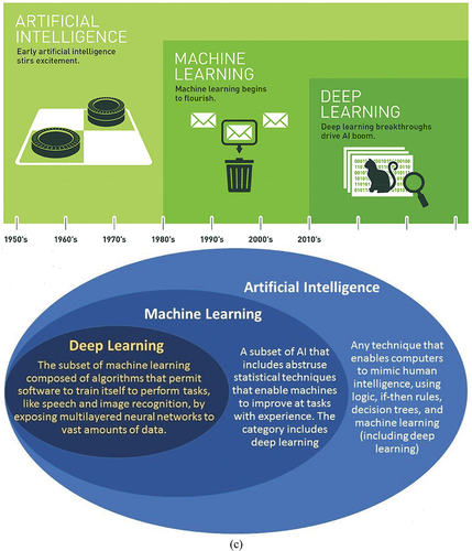
To investigate the degree of novelty of Equation (3) = ‘ARD ⊂ EO-IU ⊂ CV ⊂ AGI ⊂ Cognitive science’, depicted in Figure 11, let us recall that, as reported in this Section above, in agreement with the notion of counterfactual as hypothetical statement or question that cannot be verified or answered through observation (Heckerman & Shachter, 1995), Konrad Lorenz’ notion of thinking as acting in an imagined (mental) space (Lorenz, 1978) “ultimately requires the ability to reflect back on one’s actions and envision alternative scenarios, possibly necessitating (the illusion of) free will. The biological function of self-consciousness may be related to the need for a variable [a.k.a. agent] representing oneself in one’s Lorenzian imagined space, and free will may then be a means to communicate about actions taken by that variable, crucial for social and cultural learning, a topic which has not yet entered the stage of machine learning research although it is at the core of human intelligence” (Schölkopf et al., 2021).

This is tantamount to saying that, unlike human intelligence, where the biological function of self-consciousness, regarded as the capability of thinking back on one’s actions and envision alternative scenarios in an imagined (mental) space (Lorenz, 1978; Schölkopf et al., 2021), is required, “the narrowly focused Artificial Intelligence applications [a.k.a. Artificial Narrow Intelligence, ANI = Equation (6)(6) $x0026;\text{ANI=}[\text{DCNN}\subset \text{DL}\subset \text{ML}\text{logical0OR}\text{Traditional}\text{deductive}ArtificialIntelligencex0026;(\text{static}\text{expert}\text{systems},\text{non0adaptive}\text{to}\text{data},\text{also}\text{known}\text{as}\text{Good}\text{Old0Fashioned}x0026;ArtificialIntelligence,\text{GOFAI}]$(6) , refer to this Section below] we have today” (U.S. DARPA – Defense Advanced Research Projects Agency, 2018), not to be confused with “the more general Artificial Intelligence applications [a.k.a. Artificial General Intelligence, AGI = Equation (5)(5) $\text{lsquo}\mathrm{A}\mathrm{R}\mathrm{D}\subset \mathrm{E}\mathrm{O}\text{-}\mathrm{I}\mathrm{U}\subset \mathrm{C}\mathrm{V}\subset \mathrm{A}\mathrm{G}\mathrm{I}\leftarrow \mathrm{A}\mathrm{N}\mathrm{I}\leftarrow \mathrm{M}\mathrm{L}\supset \mathrm{D}\mathrm{L}\supset \mathrm{D}\mathrm{e}\mathrm{e}\mathrm{p}\mathrm{C}\mathrm{o}\mathrm{n}\mathrm{v}\mathrm{o}\mathrm{l}\mathrm{u}\mathrm{t}\mathrm{i}\mathrm{o}\mathrm{n}\mathrm{a}\mathrm{l}\mathrm{N}\mathrm{e}\mathrm{u}\mathrm{r}\mathrm{a}\mathrm{l}\mathrm{N}\mathrm{e}\mathrm{t}\mathrm{w}\mathrm{o}\mathrm{r}\mathrm{k}\left(\mathrm{D}\mathrm{C}\mathrm{N}\mathrm{N}\right)\text{rsquo}$(5) , refer to this Section below] we would like to create in the future” (U.S. DARPA – Defense Advanced Research Projects Agency, 2018), pursue so-called “intelligence [actually, very, very advanced statistics (Bills, 2020)] decoupled from [self-]consciousness” (Harari, 2017, p. 361), see Figure 11(a) and (b).

Reported in this Section above, a quote by John Ball is (Ball, 2021): “meaning/semantics allows ongoing generalization because it is rich content, not just labeled content. There can be many thousands of relations (of a sign) to a referent” (class of real-world objects) “in a meaning layer, but data annotations” (labeled data, supervised data, refer to the farther Subsection 3.3.3) “may only capture a single feature for a particular purpose and unsupervised data” (unlabeled data, refer to the farther Subsection 3.3.3) “is limited to the content of the source files”.

How would the ‘ML ⊃ Deep Learning (DL)-from-data’ community (see Figure11(c)) reply to these statements by John Ball? For example, in recent years, portions of the scientific community and the general public have shown increasing concern on the “politics of data labeling” in big supervised data sets gathered to train inductive ‘DL ⊂ ML’ algorithms (Crawford & Paglen, 2019; Geiger et al., 2021; Tsipras, Santurkar, Engstrom, Ilyas, & Madry, 2020). Unfortunately, no “politics of data labeling” can solve the inherent ill-posedness of any data interpretation task, involved with the collection of structured (labeled, supervised, annotated) data sets, where the data meaning is always semantics-in-context (refer to the farther Subsection 3.3.3).

Within the multi-disciplinary domain of cognitive science discussed above, where semantic relationship ‘Cognitive science ⊃ AGI ⊃ CV ⊃ EO-IU ⊃ ARD’ = Equation (3)(3) $\text{lsquo}\mathrm{A}\mathrm{R}\mathrm{D}\subset \mathrm{E}\mathrm{O}-\mathrm{I}\mathrm{U}\subset \mathrm{C}\mathrm{V}\subset \mathrm{A}\mathrm{G}\mathrm{I}\subset \mathrm{C}\mathrm{o}\mathrm{g}\mathrm{n}\mathrm{i}\mathrm{t}\mathrm{i}\mathrm{v}\mathrm{e}\mathrm{s}\mathrm{c}\mathrm{i}\mathrm{e}\mathrm{n}\mathrm{c}\mathrm{e}\text{rsquo}$(3) holds (see Figure 11), CV (a.k.a. artificial vision), synonym for inherently ill-posed scene-from-image reconstruction and understanding (a.k.a. vision) by machine (Matsuyama & Hwang, 1990), is regarded as a specialized cognitive (sub)problem of (subset-of, with inheritance) the open cognitive problem of AGI (Bills, 2020; Chollet, 2019; Dreyfus, 1965, 1991, 1992; EC – European Commission, 2019; Fjelland, 2020; Hassabis et al., 2017; Ideami, 2021; Jajal, 2018; Jordan, 2018; Mindfire Foundation, 2018; Mitchell, 2021; Practical AI, 2020; Saba, 2020c; Santoro et al., 2021; Sweeney, 2018a; Thompson, 2018; Wolski, 2020a, 2020b) (for more details about the inherent ill-posedness of the cognitive subproblem of vision, refer to the farther Subsection 4.1).

Moreover, in Figure 11(a), it is postulated that semantic relationship

(4) $\begin{array}{rl}& \text{lsquo}(Inductive/bottom\text{-}up/statisticalmodel\text{-}based)DL\text{-}from\text{-}data\subset \\ & (Inductive/bottom\text{-}up/statisticalmodel\text{-}based)ML\text{-}from\text{-}data\\ & \to AGI\supset CV\leftarrow Humanvision\text{rsquo}\end{array}$(4)

holds, where symbol ‘→’ denotes semantic relationship part-of (without inheritance) pointing from the supplier to the client, not to be confused with relationship subset-of, ‘⊃’, meaning specialization with inheritance from the superset (at left) to the subset, in agreement with symbols adopted by the standard UML for graphical modeling of object-oriented software (Fowler, 2003). In Equation (4)(4) $\begin{array}{rl}& \text{lsquo}(Inductive/bottom\text{-}up/statisticalmodel\text{-}based)DL\text{-}from\text{-}data\subset \\ & (Inductive/bottom\text{-}up/statisticalmodel\text{-}based)ML\text{-}from\text{-}data\\ & \to AGI\supset CV\leftarrow Humanvision\text{rsquo}\end{array}$(4) , hypothesis ‘Human vision → CV’ means that CV incorporates (complies with) human vision as lower bound, i.e. to become better conditioned (constrained) for numerical solution, an inherently ill-posed CV system solution is required to include by design a computational model of human vision, complying with human visual perception (Baraldi, 2017; Baraldi & Tiede, 2018a, 2018b), including visual illusion phenomena (Baraldi, 2017; Mély, Linsley, & Serre, 2018; Perez, 2018; Pessoa, 1996; Rappe, 2018) (refer to the farther Subsection 4.2).

Worth mentioning, in Figure 11(a), the RS discipline is regarded as meta-science, like engineering (Baraldi, 2017; Baraldi & Tiede, 2018a, 2018b; Couclelis, 2012). In colloquial terms, a meta-science is an “applied” science of “basic” sciences (Wikipedia, 2020b) (refer to this Section above). The goal of a meta-science is to transform observations (sensory data, true-facts) of the physical 4D geospace-time real-world, together with knowledge about the world provided by other scientific disciplines, into useful user- and context-dependent information about the world and/or solutions in the world (Couclelis, 2012; Dreyfus, 1965, 1991, 1992; Fjelland, 2020), in agreement with the increasingly popular Data-Information-Knowledge-Wisdom (DIKW) conceptual hierarchy where, typically, information is defined in terms of data, knowledge in terms of information and wisdom in terms of knowledge (Rowley, 2007; Rowley & Hartley, 2008; Wikipedia, 2020a; Zeleny, 1987, 2005; Zins, 2007), see Figure 12.

Figure 12. Adapted from (Wikipedia, 2020a). The increasingly popular Data-Information-Knowledge-Wisdom (DIKW) pyramid (Rowley, 2007; Rowley & Hartley, 2008; Wikipedia, 2020a; Zeleny, 1987, 2005; Zins, 2007), also known as the DIKW hierarchy, refers loosely to a class of models for representing purported structural and/or functional relationships between data, information, knowledge, and wisdom (Zins, 2007). Typically, “information is defined in terms of data, knowledge in terms of information and wisdom in terms of knowledge” (Rowley, 2007; Rowley & Hartley, 2008).

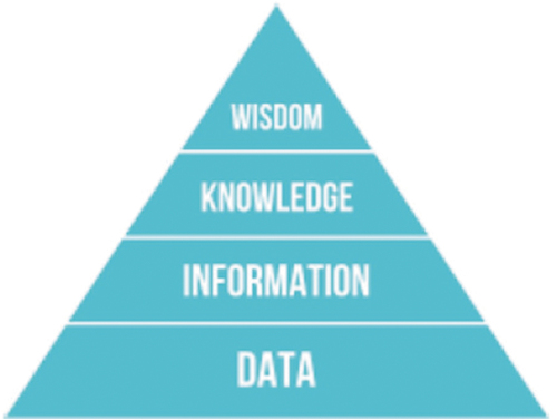
In Figure 11(a), cognitive science, regarded as superset-of AGI = Equation (2)(2) $\text{lsquo}\mathrm{C}\mathrm{o}\mathrm{g}\mathrm{n}\mathrm{i}\mathrm{t}\mathrm{i}\mathrm{v}\mathrm{e}\mathrm{s}\mathrm{c}\mathrm{i}\mathrm{e}\mathrm{n}\mathrm{c}\mathrm{e}\supset \mathrm{A}\mathrm{G}\mathrm{I}\supset \mathrm{C}\mathrm{V}\supset \mathrm{E}\mathrm{O}\text{-}\mathrm{I}\mathrm{U}\text{rsquo}$(2) , encompasses neuroscience, in particular neurophysiology, which studies the neuro-cerebral apparatus of living organisms. Neural network (NN) is synonym for distributed processing system, consisting of neurons as elementary processing units and synapses as lateral connections (Baraldi & Alpaydin, 2002a, 2002b; Buyong, 2007; Fritzke, 1997; Martinetz, Berkovich, & Schulten, 1994). Since the 1950s, the scientific community has been facing the following fundamental question (Serra & Zanarini, 1990; Westphal, 2016).

Is it possible and even convenient to mimic biological mental functions, e.g. cognitive human reasoning (Baraldi, 2017; Green et al., 2002; Kuhn, 2005; Laurini & Thompson, 1992; Matsuyama & Hwang, 1990; Newell & Simon, 1972; Sheth, 2015; Sonka et al., 1994; Sowa, 2000), by means of an artificial mind whose physical support is not an electronic brain implemented as a complex system/distributed processing system, a.k.a. artificial NN (ANN), e.g. an ANN based on the McCulloch and Pitts (MCP) neuron model, conceived almost 80 years ago as a simplified neurophysiological version of biological neurons (McCulloch & Pitts, 1943), or its improved recent versions (Cimpoi et al., 2014; Krizhevsky et al., 2012), in compliance with the mind-brain problem (Hassabis et al., 2017; Hoffman, 2008; Serra & Zanarini, 1990; Westphal, 2016)? In other words, is it possible and even convenient to search for an artificial mind independently of its physical support implemented, for example, by means of a Von Neuman machine, the basic design of the modern, or classical, computer (Britannica Online Encyclopedia, 2017), which is not an ANN?

The answer is no, according to the “connectionists approach” promoted by traditional cybernetics (Jordan, 2018; Langley, 2012), where a complex system always comprises an “artificial mind in electronic brain” paradigm (Baraldi, 2017; Serra & Zanarini, 1990; Westphal, 2016). This is alternative to a traditional approach to Artificial Narrow/Weak Intelligence (ANI) (Bills, 2020; Hassabis et al., 2017; Jajal, 2018; Mindfire Foundation, 2018; Practical AI, 2020), whose so-called symbolic/syntactic approach, typically known as GOFAI (refer to Equation (6)(6) $x0026;\text{ANI=}[\text{DCNN}\subset \text{DL}\subset \text{ML}\text{logical0OR}\text{Traditional}\text{deductive}ArtificialIntelligencex0026;(\text{static}\text{expert}\text{systems},\text{non0adaptive}\text{to}\text{data},\text{also}\text{known}\text{as}\text{Good}\text{Old0Fashioned}x0026;ArtificialIntelligence,\text{GOFAI}]$(6) in this Section below), investigates an artificial mind independently of its physical support (Baraldi, 2017; Serra & Zanarini, 1990; Westphal, 2016), see Figure 11(b).

Hence, ANI comprises as part-of (without inheritance) traditional deductive/ top-down/ learning-by-rule/ physical model-based static (non-adaptive to data) expert systems (static if-then decision trees) (Bishop, 1995; Cherkassky & Mulier, 1998; Sonka et al., 1994), often referred to as GOFAI (Dreyfus, 1965, 1991, 1992; Santoro et al., 2021), whose “attempt is to create Artificial Intelligence by applying the syntactic mechanisms developed in computer science, formal logic (Laurini & Thompson, 1992; Sowa, 2000), mathematics, physics, and psychology” (Santoro et al., 2021).

Worth observing, it is sufficient to track down the original meaning-by-convention/ semantics-in-context of the two aforementioned notions of cybernetics and Artificial Intelligence, whose origins date back not further than 1956 (Langley, 2012), to unequivocally conclude that the current interpretation of buzzword Artificial Intelligence promoted by increasing portions of both the scientific community and the general public is paradoxically affected by a transfer of meaning from the former to the latter. In the words by Michael Jordan, “it was John McCarthy (while a professor at Dartmouth, and soon to take a position at MIT) who coined the term ‘Artificial Intelligence,’ apparently to distinguish his budding research agenda from that of Norbert Wiener (then an older professor at MIT). Wiener had coined ‘cybernetics’ to refer to his own vision of intelligent systems – a vision that was closely tied to operations research, statistics, pattern recognition, information theory and control theory. McCarthy, on the other hand, emphasized the ties to logic [by now, referred to as GOFAI]. In an interesting reversal, it is Wiener’s intellectual agenda that has come to dominate in the current era [of inductive learning-from data ANNs in the realm of ML as superset-of DL], under the banner of McCarthy’s terminology” (Jordan, 2018) (for a full quote by Michael Jordan, refer to Appendix I).

In Figure 11(a) and Figure 11(b), the inherently vague/equivocal notion of Artificial Intelligence (which is one expression, with at least two meanings) is disambiguated into the two complementary (co-existing) not-alternative concepts of AGI and ANI (Bills, 2020; Chollet, 2019; Dreyfus, 1965, 1991, 1992; EC – European Commission, 2019; Fjelland, 2020; Hassabis et al., 2017; Hawkins, 2021; Ideami, 2021; Jajal, 2018; Jordan, 2018; Mindfire Foundation, 2018; Mitchell, 2021; Practical AI, 2020; Romero, 2021; Saba, 2020c; Santoro et al., 2021; Sweeney, 2018a; Thompson, 2018; Wolski, 2020a, 2020b), which are better constrained to be better understood. As original contribution of the present work, Figure 11(a) and Figure 11(b) postulate that, in the multi-disciplinary domain of cognitive science, semantic relationship

(5) $\text{lsquo}\mathrm{A}\mathrm{R}\mathrm{D}\subset \mathrm{E}\mathrm{O}\text{-}\mathrm{I}\mathrm{U}\subset \mathrm{C}\mathrm{V}\subset \mathrm{A}\mathrm{G}\mathrm{I}\leftarrow \mathrm{A}\mathrm{N}\mathrm{I}\leftarrow \mathrm{M}\mathrm{L}\supset \mathrm{D}\mathrm{L}\supset \mathrm{D}\mathrm{e}\mathrm{e}\mathrm{p}\mathrm{C}\mathrm{o}\mathrm{n}\mathrm{v}\mathrm{o}\mathrm{l}\mathrm{u}\mathrm{t}\mathrm{i}\mathrm{o}\mathrm{n}\mathrm{a}\mathrm{l}\mathrm{N}\mathrm{e}\mathrm{u}\mathrm{r}\mathrm{a}\mathrm{l}\mathrm{N}\mathrm{e}\mathrm{t}\mathrm{w}\mathrm{o}\mathrm{r}\mathrm{k}\left(\mathrm{D}\mathrm{C}\mathrm{N}\mathrm{N}\right)\text{rsquo}$(5)

holds, with ‘ARD ⊂ EO-IU ⊂ CV ⊂ AGI ⊂ Cognitive science’ = Equation (3)(3) $\text{lsquo}\mathrm{A}\mathrm{R}\mathrm{D}\subset \mathrm{E}\mathrm{O}-\mathrm{I}\mathrm{U}\subset \mathrm{C}\mathrm{V}\subset \mathrm{A}\mathrm{G}\mathrm{I}\subset \mathrm{C}\mathrm{o}\mathrm{g}\mathrm{n}\mathrm{i}\mathrm{t}\mathrm{i}\mathrm{v}\mathrm{e}\mathrm{s}\mathrm{c}\mathrm{i}\mathrm{e}\mathrm{n}\mathrm{c}\mathrm{e}\text{rsquo}$(3) and where ANI is formulated as

(6) $x0026;\text{ANI=}[\text{DCNN}\subset \text{DL}\subset \text{ML}\text{logical0OR}\text{Traditional}\text{deductive}ArtificialIntelligencex0026;(\text{static}\text{expert}\text{systems},\text{non0adaptive}\text{to}\text{data},\text{also}\text{known}\text{as}\text{Good}\text{Old0Fashioned}x0026;ArtificialIntelligence,\text{GOFAI}]$(6)

To date, it is acknowledged (at least in words) by the EC that “currently deployed Artificial Intelligence systems are examples of ANI” (EC – European Commission, 2019), in agreement with relevant portions of the scientific literature (refer to references listed in the previous paragraph of this Section).

In the words by Michael Jordan: “Most of what is being called Artificial Intelligence today, particularly in the public sphere, is what has been called ‘Machine Learning’ (ML) for the past several decades … Historically, the phrase ‘Artificial Intelligence’ was coined in the late 1950’s to refer to the heady aspiration of realizing in software and hardware an entity possessing human-level intelligence … ‘Artificial Intelligence’ was meant to focus on the ‘high-level’ or ‘cognitive’ capability of humans to ‘reason’ and to ‘think.’ Sixty years hence, however, high-level reasoning and thought remain elusive. The developments which are now being called ‘Artificial Intelligence’ arose mostly in the engineering fields associated with low-level pattern recognition and movement control, and in the field of statistics – the discipline focused on finding patterns in data and on making well-founded predictions, tests of hypotheses and decisions” (Jordan, 2018) (for a full quote by Michael Jordan, refer to Appendix I).

In agreement with these quotes, the original contribution of Equation (6)(6) $x0026;\text{ANI=}[\text{DCNN}\subset \text{DL}\subset \text{ML}\text{logical0OR}\text{Traditional}\text{deductive}ArtificialIntelligencex0026;(\text{static}\text{expert}\text{systems},\text{non0adaptive}\text{to}\text{data},\text{also}\text{known}\text{as}\text{Good}\text{Old0Fashioned}x0026;ArtificialIntelligence,\text{GOFAI}]$(6) is to propose an explicit formulation of ANI as logical-OR combination (without mixture) between, on the one hand, end-to-end inductive/ bottom-up/ statistical model-based ML-from-data algorithms (Bishop, 1995; Cherkassky & Mulier, 1998; Hassabis et al., 2017; Mindfire Foundation, 2018; Sonka et al., 1994), whose subset-of (with inheritance) is the increasingly popular DL-from-data paradigm (Cimpoi et al., 2014; Claire, 2019; Copeland, 2016; Krizhevsky et al., 2012). In the ML common practice, DL is considered equivalent to “a modern rendition of cybernetics” (Perez, 2020), where cybernetics is regarded as “connectionists approach” (Serra & Zanarini, 1990) (refer to this Section above). On the other hand, ANI comprises traditional deductive/ top-down/ learning-by-rule/ physical model-based static (non-adaptive to data) expert systems (static if-then decision trees) (Bishop, 1995; Cherkassky & Mulier, 1998; Sonka et al., 1994), often referred to as GOFAI (Dreyfus, 1965, 1991, 1992; Santoro et al., 2021).

The proposed explicit formulation of ANI = Equation (6)(6) $x0026;\text{ANI=}[\text{DCNN}\subset \text{DL}\subset \text{ML}\text{logical0OR}\text{Traditional}\text{deductive}ArtificialIntelligencex0026;(\text{static}\text{expert}\text{systems},\text{non0adaptive}\text{to}\text{data},\text{also}\text{known}\text{as}\text{Good}\text{Old0Fashioned}x0026;ArtificialIntelligence,\text{GOFAI}]$(6) is obvious (straightforward, intuitive), but not trivial. It agrees with a quote by Adam Santoro and collaborators at DeepMind, whose recent paper, unlike much of the research published by DeepMind which is largely empirical in nature, presents a philosophical perspective on the classic symbolic versus connectionist debate (Santoro et al., 2021): “ … the apparent weaknesses of current connectionist-based approaches are leading some to call for a return of symbolic methods, a de-emphasis of connectionist methods, or some reconciliation of the two. As the argument goes, perhaps it is not true that these methods alone lead to human-like intelligent action, but rather, the path towards intelligent action lies in a chimeric assembly of old methods with the new. However, here we argue that building a system that exhibits human-like engagement with symbols is not a necessary consequence of deploying ‘symbolic methods’ (which we term Good Old-Fashioned Artificial Intelligence-like, GOFAI-like), whether in conjunction with neural networks or not. This is because these (two) approaches miss much of the full spectrum of symbolic capabilities that humans exhibit.”

The original formulation of Equation (5)(5) $\text{lsquo}\mathrm{A}\mathrm{R}\mathrm{D}\subset \mathrm{E}\mathrm{O}\text{-}\mathrm{I}\mathrm{U}\subset \mathrm{C}\mathrm{V}\subset \mathrm{A}\mathrm{G}\mathrm{I}\leftarrow \mathrm{A}\mathrm{N}\mathrm{I}\leftarrow \mathrm{M}\mathrm{L}\supset \mathrm{D}\mathrm{L}\supset \mathrm{D}\mathrm{e}\mathrm{e}\mathrm{p}\mathrm{C}\mathrm{o}\mathrm{n}\mathrm{v}\mathrm{o}\mathrm{l}\mathrm{u}\mathrm{t}\mathrm{i}\mathrm{o}\mathrm{n}\mathrm{a}\mathrm{l}\mathrm{N}\mathrm{e}\mathrm{u}\mathrm{r}\mathrm{a}\mathrm{l}\mathrm{N}\mathrm{e}\mathrm{t}\mathrm{w}\mathrm{o}\mathrm{r}\mathrm{k}\left(\mathrm{D}\mathrm{C}\mathrm{N}\mathrm{N}\right)\text{rsquo}$(5) , where semantic relationship part-of (without inheritance) is proposed for ANI with respect to AGI, such that ‘ANI → AGI ⊂ Cognitive science’, agrees with Oren Etzioni’s quote that “with all due respect to the brilliant Geoff Hinton [who ‘started’ the DL hype back in 2012 (Krizhevsky et al., 2012), following his own ‘first’ invention of the back-propagation ML-from-data algorithm in 1986 (Bishop, 1995; Cherkassky & Mulier, 1998)] – thought is not a vector, and Artificial Intelligence is not a problem in statistics” (Etzioni, 2017). In fact, AGI is a problem in cognitive science, see Figure 11(a). Unlike statistics, AGI focuses on data interpretation to acquire meaning-by-convention/semantics-in-context in compliance with (constrained by) a 7D conceptual world model (refer to this Section above).

As reported above, in John Ball’s words, “what is missing from data science is meaning [semantics]” (Ball, 2021). He also considers that, “it is common to hear the question: ‘what do you mean by meaning?’ from the Artificial Intelligence community” (Ball, 2021).

These two observations read as: what is missing from both data science and currently deployed Artificial Intelligence, which is ANI (EC – European Commission, 2019), is meaning/semantics, to be regarded as meaning-by-convention/semantics-in-context (Ball, 2021; Santoro et al., 2021).

This conclusion agrees with the quote by Nicole Bills: “if you’re a nontechnical person, you can safely replace just about every use of currently deployed Artificial Intelligence, which is ANI, with very, very advanced statistics. This is certainly true for any tool available on the marketplace today. There is still room for philosophical discussion around questions of AGI, but that technology is still a long ways off” (Bills, 2020), which agrees with the aforementioned quote by Michael Jordan (for a full quote by Michael Jordan, refer to Appendix I).

With special regard to the field of Natural Language Understanding (NLU) (Expert, 2020), where NLU is regarded as subset-of AGI in analogy with ‘CV ⊂ AGI’ = Equation (5)(5) $\text{lsquo}\mathrm{A}\mathrm{R}\mathrm{D}\subset \mathrm{E}\mathrm{O}\text{-}\mathrm{I}\mathrm{U}\subset \mathrm{C}\mathrm{V}\subset \mathrm{A}\mathrm{G}\mathrm{I}\leftarrow \mathrm{A}\mathrm{N}\mathrm{I}\leftarrow \mathrm{M}\mathrm{L}\supset \mathrm{D}\mathrm{L}\supset \mathrm{D}\mathrm{e}\mathrm{e}\mathrm{p}\mathrm{C}\mathrm{o}\mathrm{n}\mathrm{v}\mathrm{o}\mathrm{l}\mathrm{u}\mathrm{t}\mathrm{i}\mathrm{o}\mathrm{n}\mathrm{a}\mathrm{l}\mathrm{N}\mathrm{e}\mathrm{u}\mathrm{r}\mathrm{a}\mathrm{l}\mathrm{N}\mathrm{e}\mathrm{t}\mathrm{w}\mathrm{o}\mathrm{r}\mathrm{k}\left(\mathrm{D}\mathrm{C}\mathrm{N}\mathrm{N}\right)\text{rsquo}$(5) , which means that both NLU and CV are “AGI-complete” problems (Saba, 2020c; Wikipedia, 2021a), Walid Saba states: “the discussion that follows is concerned with natural language understanding (NLU), namely, the task of fully comprehending (understanding) ordinary spoken language, much like humans do. We are not concerned here with what is inappropriately called natural language processing (NLP), but is really just text processing, and where text is treated as mere data (much like bits or pixels), and where data-driven approaches can perform what are essentially pattern recognition tasks, e.g. filtering, text classification, sequence-to-sequence (so-called) ‘translation’, search, clustering, etc., with some degree of ‘accuracy’ … We will present here four arguments that clearly show how fallacious is the data-driven and machine learning approaches to NLU are, and these arguments are presented in no particular order, as any one of them is actually enough on its own to put an end to this (data-driven/ML) futile effort … Finally, a plea: some sanity is needed in the field of NLU, before we spend too much time and effort travelling along the wrong path. The ‘chasing infinity’ data-driven/ML approach to NLU is a futile effort, and it is time to take this very challenging task out of the hands of hackers before more time and resources are spent in vain” (Saba, 2020c) (for a full quote by Walid Saba, refer to Appendix I).

In Pat Langley’s words: “The early days of Artificial Intelligence were guided by a common vision: understanding and reproducing, in computational systems, the full range of intelligent behavior that we observe in humans. Many researchers continued to share these aims from arguably the foundation of the 1956 Artificial Intelligence revolution until the 1980s and 1990s, when Artificial Intelligence began to fragment into a variety of specialized subdisciplines, each with far more limited objectives. This produced progress in each area, but, in the process, many abandoned the field’s original goal. Rather than creating intelligent systems with the same breadth and flexibility as humans, most recent research has produced impressive but narrow idiot savants … Most Artificial Intelligence courses ignore the cognitive systems perspective … Instead, we must provide a broad education in Artificial Intelligence that cuts across different topics to cover all the field’s branches and their role in intelligent systems … from cognitive psychology, linguistics, and logic, which are far more important to the cognitive systems agenda than ones from mainstream computer science” (Langley, 2012).

In 2017, DeepMind’s Demis Hassabis and co-authors observed that “for centuries, human intelligence has been the basic inspiration for the creation of intelligent machines. Hence, the creation of intelligent machines has been closely connected with research fields studying natural intelligence, particularly human intelligence, like neuroscience and psychology. However, there has since been a drift away from this essential exchange and collaboration between artificial and natural intelligence research for the creation of AGI … The search space of possible solutions [to intelligence] is vast and likely only very sparsely populated … this therefore underscores the utility of scrutinizing the inner workings of the human brain – the only existing proof that such an intelligence is even possible” (Hassabis et al., 2017).

In an agile approach to product development, Jan Zawadzki points out that “Artificial Intelligence product teams need a variety of skills, and not only Data Scientists” (Zawadzki, 2021). Based on Figure 11, our revised version of Jan Zawadzki’s recommendation would read as: “Artificial [General] Intelligence product teams need a variety of skills, encompassing the multi-disciplinary domain of cognitive science, and not only Data Scientists”.

In spite of the endorsement (at least in words) by the EC (EC – European Commission, 2019), in agreement with relevant portions of the scientific literature (refer to references listed in this Section above), the original formulation of Equation (5)(5) $\text{lsquo}\mathrm{A}\mathrm{R}\mathrm{D}\subset \mathrm{E}\mathrm{O}\text{-}\mathrm{I}\mathrm{U}\subset \mathrm{C}\mathrm{V}\subset \mathrm{A}\mathrm{G}\mathrm{I}\leftarrow \mathrm{A}\mathrm{N}\mathrm{I}\leftarrow \mathrm{M}\mathrm{L}\supset \mathrm{D}\mathrm{L}\supset \mathrm{D}\mathrm{e}\mathrm{e}\mathrm{p}\mathrm{C}\mathrm{o}\mathrm{n}\mathrm{v}\mathrm{o}\mathrm{l}\mathrm{u}\mathrm{t}\mathrm{i}\mathrm{o}\mathrm{n}\mathrm{a}\mathrm{l}\mathrm{N}\mathrm{e}\mathrm{u}\mathrm{r}\mathrm{a}\mathrm{l}\mathrm{N}\mathrm{e}\mathrm{t}\mathrm{w}\mathrm{o}\mathrm{r}\mathrm{k}\left(\mathrm{D}\mathrm{C}\mathrm{N}\mathrm{N}\right)\text{rsquo}$(5) and Equation (6)(6) $x0026;\text{ANI=}[\text{DCNN}\subset \text{DL}\subset \text{ML}\text{logical0OR}\text{Traditional}\text{deductive}ArtificialIntelligencex0026;(\text{static}\text{expert}\text{systems},\text{non0adaptive}\text{to}\text{data},\text{also}\text{known}\text{as}\text{Good}\text{Old0Fashioned}x0026;ArtificialIntelligence,\text{GOFAI}]$(6) cannot be considered either trivial or community-agreed upon. In more detail, AGI = Equation (5)(5) $\text{lsquo}\mathrm{A}\mathrm{R}\mathrm{D}\subset \mathrm{E}\mathrm{O}\text{-}\mathrm{I}\mathrm{U}\subset \mathrm{C}\mathrm{V}\subset \mathrm{A}\mathrm{G}\mathrm{I}\leftarrow \mathrm{A}\mathrm{N}\mathrm{I}\leftarrow \mathrm{M}\mathrm{L}\supset \mathrm{D}\mathrm{L}\supset \mathrm{D}\mathrm{e}\mathrm{e}\mathrm{p}\mathrm{C}\mathrm{o}\mathrm{n}\mathrm{v}\mathrm{o}\mathrm{l}\mathrm{u}\mathrm{t}\mathrm{i}\mathrm{o}\mathrm{n}\mathrm{a}\mathrm{l}\mathrm{N}\mathrm{e}\mathrm{u}\mathrm{r}\mathrm{a}\mathrm{l}\mathrm{N}\mathrm{e}\mathrm{t}\mathrm{w}\mathrm{o}\mathrm{r}\mathrm{k}\left(\mathrm{D}\mathrm{C}\mathrm{N}\mathrm{N}\right)\text{rsquo}$(5) and ANI = Equation (6)(6) $x0026;\text{ANI=}[\text{DCNN}\subset \text{DL}\subset \text{ML}\text{logical0OR}\text{Traditional}\text{deductive}ArtificialIntelligencex0026;(\text{static}\text{expert}\text{systems},\text{non0adaptive}\text{to}\text{data},\text{also}\text{known}\text{as}\text{Good}\text{Old0Fashioned}x0026;ArtificialIntelligence,\text{GOFAI}]$(6) , summarized as working hypothesis ‘AGI ← ANI ← ML ⊃ DL ⊃ DCNN’, are alternative to (inconsistent with) the increasingly popular postulate (axiom) that relationship

(7) $\text{lsquo}\mathrm{A}(\mathrm{G}/\mathrm{N})\mathrm{I}\supset \mathrm{M}\mathrm{L}\supset \mathrm{D}\mathrm{L}\supset \mathrm{D}\mathrm{C}\mathrm{N}\mathrm{N}\text{rsquo}$(7)

holds (Claire, 2019; Copeland, 2016), see Figure 11(c). For example, in (Copeland, 2016), it is reported that: “since an early flush of optimism in the 1950s, smaller subsets of Artificial Intelligence – first machine learning, then deep learning, a subset of machine learning – have created even larger disruptions.” Moreover, starting from 2012, when the ‘DL ⊂ ML’ paradigm was successfully proposed by the CV community (Krizhevsky et al., 2012), DL enthusiasts, practitioners and scientists have been promoting DL as synonym for A(G/N)I (Claire, 2019; Copeland, 2016), rather than as synonym for “very, very advanced statistics”, as recommended in (Bills, 2020).

Although popular in recent days, axiom ‘A(G/N)I ⊃ ML ⊃ DL ⊃ DCNN’ = Equation (7)(7) $\text{lsquo}\mathrm{A}(\mathrm{G}/\mathrm{N})\mathrm{I}\supset \mathrm{M}\mathrm{L}\supset \mathrm{D}\mathrm{L}\supset \mathrm{D}\mathrm{C}\mathrm{N}\mathrm{N}\text{rsquo}$(7) is in contrast with the early days of ML, when scientists never confused ML with AGI, i.e. relationship ‘ML ⊂ AGI’ was never promoted (Bishop, 1995; Cherkassky & Mulier, 1998; Geman et al., 1992; Mahadevan, 2019; Russell & Norvig, 1995; Wolpert, 1996).

To date, increasing disillusionment on ‘DL ⊂ ML → ANI → AGI’ (Bartoš, 2017; Bills, 2020; Bourdakos, 2017; Brendel, 2019; Brendel & Bethge, 2019; Chollet, 2019; Crawford & Paglen, 2019; Deutsch, 2012; Dreyfus, 1965, 1991, 1992; Etzioni, 2017; Expert.ai, 2020; Fjelland, 2020; Geman et al., 1992; Gonfalonieri, 2020; Hao, 2019; Hassabis et al., 2017; Hawkins, 2021; Ideami, 2021; Jordan, 2018; Langley, 2012; LeVine, 2017; Lohr, 2018; Lukianoff, 2019; Mahadevan, 2019; Marcus, 2018, 2020; Marks, 2021; Mindfire Foundation, 2018; Mitchell, 2019, 2021; Nguyen et al., 2014; Pearl & Mackenzie, 2018; Peng, 2017; Perez, 2017; Pfeffer, 2018; Practical AI, 2020; Rahimi, 2017; Romero, 2021; Russell & Norvig, 1995; Saba, 2020c; Santoro et al., 2021; Strubell et al., 2019; Sweeney, 2018a, 2018b; Szegedy et al., 2013; Thompson, 2018; U.S. DARPA – Defense Advanced Research Projects Agency, 2018; Wolpert, 1996; Wolpert & Macready, 1997; Wolski, 2020a, 2020b; Ye, 2020; Yuille & Liu, 2019; Zador, 2019) mainly stems from portions of the ML community pre-dating the recent popularity of DL (Claire, 2019; Copeland, 2016; Krizhevsky et al., 2012). To quote one of the best-known ML pioneers, Stuart Russell (Bills, 2020; Practical AI, 2020): “I don’t think DL evolves into Artificial General Intelligence (AGI). AGI is not going to be reached by just having bigger DL networks and more data … DL systems don’t know anything, they can’t reason, and they can’t accumulate knowledge, they can’t apply what they learned in one context to solve problems in another context, etc. And these are just elementary things that humans do all the time.”

In contrast with the recent hype on Equation (7)(7) $\text{lsquo}\mathrm{A}(\mathrm{G}/\mathrm{N})\mathrm{I}\supset \mathrm{M}\mathrm{L}\supset \mathrm{D}\mathrm{L}\supset \mathrm{D}\mathrm{C}\mathrm{N}\mathrm{N}\text{rsquo}$(7) , a few more quotes of interest by Alberto Romero (Romero, 2021), Walid Saba (Saba, 2020c), Michael Jordan (Jordan, 2018), Oren Etzioni (Etzioni, 2017), Stuart Russell (Bills, 2020; Practical AI, 2020), Pat Langley (Langley, 2012), EC (EC – European Commission, 2019), Melanie Mitchell (Mitchell, 2019), Geoffrey Hinton (LeVine, 2017), Ali Rahimi (Pfeffer, 2018; Rahimi, 2017), Maciej Wolski (Wolski, 2020a, 2020b) and Karen Hao (Hao, 2019; Strubell et al., 2019) are reported in Appendix I for the sake of completeness, because these relevant contributions are enigmatically ignored, to date, by meta-sciences like engineering and RS.

Two important takeaways from quotes reported in Appendix I are proposed hereafter as useful synonyms. They are short and intuitive, therefore easy to remember.

First, synonym for DL is “very, very advanced statistics” (Bills, 2020), where ‘DL ⊂ ML → ANI → AGI’ = Equation (5)(5) $\text{lsquo}\mathrm{A}\mathrm{R}\mathrm{D}\subset \mathrm{E}\mathrm{O}\text{-}\mathrm{I}\mathrm{U}\subset \mathrm{C}\mathrm{V}\subset \mathrm{A}\mathrm{G}\mathrm{I}\leftarrow \mathrm{A}\mathrm{N}\mathrm{I}\leftarrow \mathrm{M}\mathrm{L}\supset \mathrm{D}\mathrm{L}\supset \mathrm{D}\mathrm{e}\mathrm{e}\mathrm{p}\mathrm{C}\mathrm{o}\mathrm{n}\mathrm{v}\mathrm{o}\mathrm{l}\mathrm{u}\mathrm{t}\mathrm{i}\mathrm{o}\mathrm{n}\mathrm{a}\mathrm{l}\mathrm{N}\mathrm{e}\mathrm{u}\mathrm{r}\mathrm{a}\mathrm{l}\mathrm{N}\mathrm{e}\mathrm{t}\mathrm{w}\mathrm{o}\mathrm{r}\mathrm{k}\left(\mathrm{D}\mathrm{C}\mathrm{N}\mathrm{N}\right)\text{rsquo}$(5) holds.

Second, synonym for ANI = Equation (6)(6) $x0026;\text{ANI=}[\text{DCNN}\subset \text{DL}\subset \text{ML}\text{logical0OR}\text{Traditional}\text{deductive}ArtificialIntelligencex0026;(\text{static}\text{expert}\text{systems},\text{non0adaptive}\text{to}\text{data},\text{also}\text{known}\text{as}\text{Good}\text{Old0Fashioned}x0026;ArtificialIntelligence,\text{GOFAI}]$(6) is “narrow idiot savant” (Langley, 2012).

To recap, our present work is alternative to the recent hype on DL and in contrast with the popular assumption that Equation (7)(7) $\text{lsquo}\mathrm{A}(\mathrm{G}/\mathrm{N})\mathrm{I}\supset \mathrm{M}\mathrm{L}\supset \mathrm{D}\mathrm{L}\supset \mathrm{D}\mathrm{C}\mathrm{N}\mathrm{N}\text{rsquo}$(7) holds. Adopted as original working hypotheses in the rest of this paper, semantic relationships AGI = Equation (5)(5) $\text{lsquo}\mathrm{A}\mathrm{R}\mathrm{D}\subset \mathrm{E}\mathrm{O}\text{-}\mathrm{I}\mathrm{U}\subset \mathrm{C}\mathrm{V}\subset \mathrm{A}\mathrm{G}\mathrm{I}\leftarrow \mathrm{A}\mathrm{N}\mathrm{I}\leftarrow \mathrm{M}\mathrm{L}\supset \mathrm{D}\mathrm{L}\supset \mathrm{D}\mathrm{e}\mathrm{e}\mathrm{p}\mathrm{C}\mathrm{o}\mathrm{n}\mathrm{v}\mathrm{o}\mathrm{l}\mathrm{u}\mathrm{t}\mathrm{i}\mathrm{o}\mathrm{n}\mathrm{a}\mathrm{l}\mathrm{N}\mathrm{e}\mathrm{u}\mathrm{r}\mathrm{a}\mathrm{l}\mathrm{N}\mathrm{e}\mathrm{t}\mathrm{w}\mathrm{o}\mathrm{r}\mathrm{k}\left(\mathrm{D}\mathrm{C}\mathrm{N}\mathrm{N}\right)\text{rsquo}$(5) and ANI = Equation (6)(6) $x0026;\text{ANI=}[\text{DCNN}\subset \text{DL}\subset \text{ML}\text{logical0OR}\text{Traditional}\text{deductive}ArtificialIntelligencex0026;(\text{static}\text{expert}\text{systems},\text{non0adaptive}\text{to}\text{data},\text{also}\text{known}\text{as}\text{Good}\text{Old0Fashioned}x0026;ArtificialIntelligence,\text{GOFAI}]$(6) are, first, in contrast with the increasingly popular postulate that Equation (7)(7) $\text{lsquo}\mathrm{A}(\mathrm{G}/\mathrm{N})\mathrm{I}\supset \mathrm{M}\mathrm{L}\supset \mathrm{D}\mathrm{L}\supset \mathrm{D}\mathrm{C}\mathrm{N}\mathrm{N}\text{rsquo}$(7) holds (Claire, 2019; Copeland, 2016), see Figure 11. Second, AGI = Equation (5)(5) $\text{lsquo}\mathrm{A}\mathrm{R}\mathrm{D}\subset \mathrm{E}\mathrm{O}\text{-}\mathrm{I}\mathrm{U}\subset \mathrm{C}\mathrm{V}\subset \mathrm{A}\mathrm{G}\mathrm{I}\leftarrow \mathrm{A}\mathrm{N}\mathrm{I}\leftarrow \mathrm{M}\mathrm{L}\supset \mathrm{D}\mathrm{L}\supset \mathrm{D}\mathrm{e}\mathrm{e}\mathrm{p}\mathrm{C}\mathrm{o}\mathrm{n}\mathrm{v}\mathrm{o}\mathrm{l}\mathrm{u}\mathrm{t}\mathrm{i}\mathrm{o}\mathrm{n}\mathrm{a}\mathrm{l}\mathrm{N}\mathrm{e}\mathrm{u}\mathrm{r}\mathrm{a}\mathrm{l}\mathrm{N}\mathrm{e}\mathrm{t}\mathrm{w}\mathrm{o}\mathrm{r}\mathrm{k}\left(\mathrm{D}\mathrm{C}\mathrm{N}\mathrm{N}\right)\text{rsquo}$(5) and ANI = Equation (6)(6) $x0026;\text{ANI=}[\text{DCNN}\subset \text{DL}\subset \text{ML}\text{logical0OR}\text{Traditional}\text{deductive}ArtificialIntelligencex0026;(\text{static}\text{expert}\text{systems},\text{non0adaptive}\text{to}\text{data},\text{also}\text{known}\text{as}\text{Good}\text{Old0Fashioned}x0026;ArtificialIntelligence,\text{GOFAI}]$(6) agree with an increasing disillusionment on ‘DL ⊂ ML → ANI → AGI’, mainly stemming from portions of the ML community pre-dating the recent popularity of DL, which has been enigmatically ignored to date by meta-sciences like engineering and RS. Third, AGI = Equation (5)(5) $\text{lsquo}\mathrm{A}\mathrm{R}\mathrm{D}\subset \mathrm{E}\mathrm{O}\text{-}\mathrm{I}\mathrm{U}\subset \mathrm{C}\mathrm{V}\subset \mathrm{A}\mathrm{G}\mathrm{I}\leftarrow \mathrm{A}\mathrm{N}\mathrm{I}\leftarrow \mathrm{M}\mathrm{L}\supset \mathrm{D}\mathrm{L}\supset \mathrm{D}\mathrm{e}\mathrm{e}\mathrm{p}\mathrm{C}\mathrm{o}\mathrm{n}\mathrm{v}\mathrm{o}\mathrm{l}\mathrm{u}\mathrm{t}\mathrm{i}\mathrm{o}\mathrm{n}\mathrm{a}\mathrm{l}\mathrm{N}\mathrm{e}\mathrm{u}\mathrm{r}\mathrm{a}\mathrm{l}\mathrm{N}\mathrm{e}\mathrm{t}\mathrm{w}\mathrm{o}\mathrm{r}\mathrm{k}\left(\mathrm{D}\mathrm{C}\mathrm{N}\mathrm{N}\right)\text{rsquo}$(5) and ANI = Equation (6)(6) $x0026;\text{ANI=}[\text{DCNN}\subset \text{DL}\subset \text{ML}\text{logical0OR}\text{Traditional}\text{deductive}ArtificialIntelligencex0026;(\text{static}\text{expert}\text{systems},\text{non0adaptive}\text{to}\text{data},\text{also}\text{known}\text{as}\text{Good}\text{Old0Fashioned}x0026;ArtificialIntelligence,\text{GOFAI}]$(6) agree with the nomenclature endorsed (at least in words) by the EC (EC – European Commission, 2019), together with relevant portions of the scientific literature (refer to references listed in this Section above).

Hence, our original work complies with the quote by Adriano Olivetti, an Italian engineer, politician and industrialist, who said: “ … All together (as a close-knit community) we will try to imagine the future, to see it. Because only if we are able to see and imagine it, will we be able to reach it” (Merola, 2014). In the multi-disciplinary context of cognitive science (see Figure 11), this sentence means that open problems, like AGI, are not solved by being ignored. Only if we today agree on the yet-unaccomplished notion (open problem) of ‘AGI ⊂ Cognitive science’, we will be able to reach it.

This consideration fully complies with the words by the Mindfire Foundation, dating back to 2018: “the research and funding focus on ANI systems could not considerably advance the progress in the direction of AGI” (Mindfire Foundation, 2018).

It agrees with the thesis proposed in 2017 by DeepMind’s Demis Hassabis and co-authors who discussed the ongoing loss of the essential exchange and collaboration between artificial and natural intelligence research for the creation of AGI, which underlines “the utility of scrutinizing the inner workings of the human brain – the only existing proof that such an intelligence is even possible” (Hassabis et al., 2017).

It also agrees with the quote by John Ball: “Rather than throw away the science of linguistics” as special case of traditional symbolic/syntactic approaches investigating an artificial mind independently of its physical support (Baraldi, 2017; Serra & Zanarini, 1990; Westphal, 2016), also referred to as GOFAI (refer to this Section above), “in favor of statistical solutions that have major limitations, let’s keep revising the science and investigating further to find workable models that deal with the perceived problems, if possible, and also address any other unsolved problems at the same time. We owe it to the next generation of linguists and cognitive scientists to show our known pros and cons to students, so they can consider solutions outside of the current models” (Ball, 2021).

Starting from Equation (5)(5) $\text{lsquo}\mathrm{A}\mathrm{R}\mathrm{D}\subset \mathrm{E}\mathrm{O}\text{-}\mathrm{I}\mathrm{U}\subset \mathrm{C}\mathrm{V}\subset \mathrm{A}\mathrm{G}\mathrm{I}\leftarrow \mathrm{A}\mathrm{N}\mathrm{I}\leftarrow \mathrm{M}\mathrm{L}\supset \mathrm{D}\mathrm{L}\supset \mathrm{D}\mathrm{e}\mathrm{e}\mathrm{p}\mathrm{C}\mathrm{o}\mathrm{n}\mathrm{v}\mathrm{o}\mathrm{l}\mathrm{u}\mathrm{t}\mathrm{i}\mathrm{o}\mathrm{n}\mathrm{a}\mathrm{l}\mathrm{N}\mathrm{e}\mathrm{u}\mathrm{r}\mathrm{a}\mathrm{l}\mathrm{N}\mathrm{e}\mathrm{t}\mathrm{w}\mathrm{o}\mathrm{r}\mathrm{k}\left(\mathrm{D}\mathrm{C}\mathrm{N}\mathrm{N}\right)\text{rsquo}$(5) = ‘DL ⊂ ML → ANI → AGI ⊃ CV ⊃ EO-IU ⊃ ARD’, depicted in Figure 11(a) and Figure 11(b), let us focus our scientific attention on imagery, synonym for 2D gridded data belonging to an image-plane (Baraldi, 2017; Matsuyama & Hwang, 1990; Van der Meer & De Jong, 2011; Victor, 1994), as a specific instantiation of sensory data at the base of the DIKW pyramid, shown in Figure 12. It means that all images are data, but not all data are imagery. Hence, not all AGI solutions are expected to perform “well” (in terms of multi-objective optimization of an mDMI set of OP-Q²Is, refer to this Section above) when input with imagery, but CV solutions as subset-of AGI specialized on image interpretation. This is tantamount to saying that popular ‘ML → ANI → AGI’ solutions suitable for coping with a 1D vector data sequence as input, such as the multi-layer perceptron, support vector machine, random forest, etc. (Bishop, 1995; Cherkassky & Mulier, 1998; Sonka et al., 1994), are inherently unfitted to deal with input (2D) imagery, due to data dimensionality reduction from 2D to 1D, which causes a total loss of the 2D spatial topology information component (Baraldi, 2017; Buyong, 2007; OGC – Open Geospatial Consortium Inc, 2015). In practice, when adopted for CV tasks, popular ‘ML → AGI’ solutions requiring a 1D vector data sequence as input, either pixel-based (2D spatial context-insensitive) or local window-based, equivalent to 1D analysis of (2D) imagery, are always affected by non-retinotopic data mapping, i.e. they are 2D spatial topology non-preserving (Baraldi, 2017; Baraldi & Alpaydin, 2002a, 2002b; Fritzke, 1997; Martinetz et al., 1994; Öğmen & Herzog, 2010; Tsotsos, 1990), in contrast with biological vision systems (DiCarlo, 2017; Dubey et al., 2018; Heitger et al., 1992; Kosslyn, 1994; Marr, 1982; Mason & Kandel, 1991; Mély et al., 2018; Öğmen & Herzog, 2010; Perez, 2018; Pessoa, 1996; Piasini et al., 2021; Rappe, 2018; Rodrigues & Du Buf, 2009; Slotnick et al., 2005; Tsotsos, 1990; Vecera & Farah, 1997; Victor, 1994).

Unfortunately, the majority of papers published in the RS literature to date adopt non-retinotopic 1D data analysis approaches, either pixel-based or local window-based, to accomplish (2D) image analysis; therefore, they are affected by a total loss of the 2D spatial topology information component. In practice, a large portion of papers published in the RS literature adopts no CV approach, capable of 2D spatial analysis of (2D) imagery.

By reversed reasoning, the previous paragraph means that ‘ARD ⊂ EO-IU ⊂ CV ⊂ AGI’ solutions, specialized on the cognitive task of vision, synonym for scene-from-image reconstruction and understanding (Matsuyama & Hwang, 1990), cannot perform “well” on input data different from still (2D) imagery or imagery-through-time (videos) (Piasini et al., 2021), in perfect analogy with the human visual (sub)system, capable of biological vision exclusively (DiCarlo, 2017; Dubey et al., 2018; Heitger et al., 1992; Kosslyn, 1994; Marr, 1982; Mason & Kandel, 1991; Mély et al., 2018; Öğmen & Herzog, 2010; Perez, 2018; Pessoa, 1996; Piasini et al., 2021; Rappe, 2018; Rodrigues & Du Buf, 2009; Slotnick et al., 2005; Tsotsos, 1990; Vecera & Farah, 1997; Victor, 1994).

Before reaching conclusions about RTD opportunities stemming from our original ‘ARD ⊂ EO-IU ⊂ CV ⊂ AGI ⊂ Cognitive science’ problem identification, let us recall here that the intuitive general-purpose GIGO principle (Baraldi, 2017; Geiger et al., 2021; Thompson, 2018) (refer to this Section above) is synonym for error (uncertainty) propagation through a data and information processing chain, such as an ‘ARD ⊂ EO-IU ⊂ CV ⊂ AGI’ workflow. The formal version of the intuitive GIGO principle is the scientific process of uncertainty (vice versa, veracity) estimation, based on a combination of the propagation law of uncertainty with the mathematical model of causality for the input-output data mapping (data link) at hand (Zhaoning et al., 2020), according to the Guide to the Expression of Uncertainty in Measurement (JCGM – Joint Committee for Guides in Metrology, 2008) and the International Vocabulary of Metrology (JCGM – Joint Committee for Guides in Metrology, 2012) criteria issued by the Joint Committee for Guides in Metrology (refer to this Section, above). Uncertainty estimation at each processing stage of an EO data-derived VAPS workflow is also considered mandatory by the intergovernmental GEO-CEOS QA4EO Cal/Val guidelines (refer to this Section above).

In compliance with an intuitive general-purpose GIGO principle (refer to references listed in this Section above), the standard FAIR criteria for scientific data (product and process) management (GO FAIR – International Support and Coordination Office, 2021; Wilkinson et al., 2016), see Table 1and the intergovernmental GEO-CEOS QA4EO Cal/Val requirements (refer to references listed in this Section above), to be included in a community-agreed mDMI set of OP-Q²Is (refer to this Section above), the potential impact upon a “seamless chain of innovation” required by a new era of Space Economy 4.0 (Mazzucato & Robinson, 2017) (see Figure 10) of a proposed innovative ‘ARD ⊂ EO-IU ⊂ CV ⊂ AGI’ system in operational mode (according to the definition provided in this Section above), suitable for multi-sensor, systematic, timely and comprehensive generation of an ambitious (suitable), but realistic (feasible, doable, viable) semantics-enriched ARD co-product pair (refer to this Section above) at the space segment and/or midstream segment (see Figure 10), is expected to be twofold.

1. In agreement with the engineering principles of modularity, hierarchy and regularity, neither necessary nor sufficient, but highly recommended for system scalability (Lipson, 2007), an innovative ‘ARD ⊂ EO-IU ⊂ CV ⊂ AGI’ (sub)system accomplished in operational mode at the space segment and/or midstream segment is regarded as necessary-but-not-sufficient precondition for developing an integrated “horizontal” (enabling) ‘AGI4DIAS = (AGI ⊃ CV ⊃ EO-IU ⊃ ARD) + DIAS 1.0 + SCBIR + SEIKD = DIAS 2.0’ = Equation (1)(1) $\begin{array}{rl}& \text{lsquo}\mathrm{A}\mathrm{G}\mathrm{I}\text{-}\mathrm{e}\mathrm{n}\mathrm{a}\mathrm{b}\mathrm{l}\mathrm{e}\mathrm{d}\mathrm{D}\mathrm{I}\mathrm{A}\mathrm{S}=\mathrm{A}\mathrm{G}\mathrm{I}4\mathrm{D}\mathrm{I}\mathrm{A}\mathrm{S}=\mathrm{S}\mathrm{e}\mathrm{m}\mathrm{a}\mathrm{n}\mathrm{t}\mathrm{i}\mathrm{c}\mathrm{s}\text{-}\mathrm{e}\mathrm{n}\mathrm{a}\mathrm{b}\mathrm{l}\mathrm{e}\mathrm{d}\mathrm{D}\mathrm{I}\mathrm{A}\mathrm{S}2.0\\ & (\mathrm{D}\mathrm{I}\mathrm{A}\mathrm{S}{2}^{\mathrm{n}\mathrm{d}}\mathrm{g}\mathrm{e}\mathrm{n}\mathrm{e}\mathrm{r}\mathrm{a}\mathrm{t}\mathrm{i}\mathrm{o}\mathrm{n})=\mathrm{D}\mathrm{I}\mathrm{A}\mathrm{S}2.0=\mathrm{A}\mathrm{G}\mathrm{I}+\mathrm{D}\mathrm{I}\mathrm{A}\mathrm{S}1.0+\mathrm{S}\mathrm{C}\mathrm{B}\mathrm{I}\mathrm{R}+\mathrm{S}\mathrm{E}\mathrm{I}\mathrm{K}\mathrm{D}\text{rsquo}\end{array}$(1) infrastructure at the midstream segment, coping with background conditions necessary to specialization occurring at the downstream segment, see Figure 10.

   Synonym for semantics-enabled EO big raster-based (numerical) data and vector-based categorical (either subsymbolic, semi-symbolic or symbolic, refer to this Section above) information cube (Augustin et al., 2018, 2019; Baraldi et al., 2016, 2017; FFG – Austrian Research Promotion Agency, 2015, 2016, 2018, 2020; Sudmanns et al., 2018; Tiede et al., 2017), the notion of AGI4DIAS is ambitious (suitable), but realistic (feasible, doable). It is proposed as viable alternative to existing EO (raster-based) big data cube management systems (Open Data Cube, 2020; Baumann, 2017; CEOS – Committee on Earth Observation Satellites, 2020; Giuliani et al., 2017, 2020; Lewis et al., 2017; Strobl et al., 2017), including the EC DIAS 1.0 realizations (EU – European Union, 2017, 2018) and the prototypical CBIR systems (Datta et al., 2008; Kumar et al., 2011; Ma & Manjunath, 1997; Shyu et al., 2007; Smeulders et al., 2000; Smith & Chang, 1996; Tyagi, 2017) (see Figure 4), typically affected by the DRIP syndrome because they lack an integrated ‘AGI ⊃ CV ⊃ EO-IU’ capability required to transform at the edge (Intelligent Edge Conference, 2021), as close as possible to EO sensory data acquisition at the space segment, quantitative/unequivocal EO large image databases into inherently ill-posed/ qualitative/ equivocal information-as-data-interpretation (Capurro & Hjørland, 2003), provided with meaning-by-convention/semantics-in-context (Ball, 2021; Peirce, 1994; Perez, 2020, 2021; Salad, 2019; Santoro et al., 2021; Wikipedia, 2021e).

   Noteworthy, the notion of AGI4DIAS fully complies with the GEO second mandate of a GEOSS for years 2016–2025 (GEO – Group on Earth Observations, 2015) (see Figure 1), expected to evolve from an EO big data sharing infrastructure, intuitively referred to as data-centric approach (Nativi et al., 2020), to an expert EO data-derived information and knowledge system (Nativi et al., 2015, pp. 7, 22), intuitively referred to as knowledge-driven approach (Nativi et al., 2020), capable of supporting decision-making by delivering to end-users high-level Essential (Community) Variables, rather than low-level EO big sensory data, to successfully cope with challenges along all six community-agreed degrees (dimensionalities, axes) of complexity of big data, known as the six Vs of volume, variety, veracity, velocity, volatility and value (Metternicht et al., 2020) (refer to this Section above), in compliance with the well-known DIKW hierarchical conceptualization, see Figure 12.

   The ambitious, but realistic RTD of an innovative semantics-enabled AGI4DIAS infrastructure at the midstream segment in a new notion of Space Economy 4.0 is of potential interest to all present and future EO large image database providers, either private, e.g. Planet (Houborga & McCabe, 2018; Planet, 2017, 2018, 2019), Maxar (Maxar, 2021; Pacifici, 2016; Pacifici et al., 2014), BlackSky, etc., or public, e.g. ESA (DLR – Deutsches Zentrum für Luft-und Raumfahrt e.V. and VEGA Technologies, 2011; ESA – European Space Agency, 2015), USGS (Dwyer et al., 2018; USGS – U.S. Geological Survey, 2018a, 2018c), NASA (NASA – National Aeronautics and Space Administration, 2019; Helder et al., 2018), etc.

2. Availability of an innovative “horizontal” (enabling) ‘AGI4DIAS = (AGI ⊃ CV ⊃ EO-IU ⊃ ARD) + DIAS 1.0 + SCBIR + SEIKD = DIAS 2.0’ = Equation (1)(1) $\begin{array}{rl}& \text{lsquo}\mathrm{A}\mathrm{G}\mathrm{I}\text{-}\mathrm{e}\mathrm{n}\mathrm{a}\mathrm{b}\mathrm{l}\mathrm{e}\mathrm{d}\mathrm{D}\mathrm{I}\mathrm{A}\mathrm{S}=\mathrm{A}\mathrm{G}\mathrm{I}4\mathrm{D}\mathrm{I}\mathrm{A}\mathrm{S}=\mathrm{S}\mathrm{e}\mathrm{m}\mathrm{a}\mathrm{n}\mathrm{t}\mathrm{i}\mathrm{c}\mathrm{s}\text{-}\mathrm{e}\mathrm{n}\mathrm{a}\mathrm{b}\mathrm{l}\mathrm{e}\mathrm{d}\mathrm{D}\mathrm{I}\mathrm{A}\mathrm{S}2.0\\ & (\mathrm{D}\mathrm{I}\mathrm{A}\mathrm{S}{2}^{\mathrm{n}\mathrm{d}}\mathrm{g}\mathrm{e}\mathrm{n}\mathrm{e}\mathrm{r}\mathrm{a}\mathrm{t}\mathrm{i}\mathrm{o}\mathrm{n})=\mathrm{D}\mathrm{I}\mathrm{A}\mathrm{S}2.0=\mathrm{A}\mathrm{G}\mathrm{I}+\mathrm{D}\mathrm{I}\mathrm{A}\mathrm{S}1.0+\mathrm{S}\mathrm{C}\mathrm{B}\mathrm{I}\mathrm{R}+\mathrm{S}\mathrm{E}\mathrm{I}\mathrm{K}\mathrm{D}\text{rsquo}\end{array}$(1) infrastructure at the midstream segment, coping with background conditions necessary to specialization, is regarded as necessary-but-not-sufficient precondition for the downstream service and application industry to develop an ever-increasing ensemble of “vertical” (deep and narrow, specialized) user- and application-specific VAPS in operational mode, suitable for use by a potentially huge worldwide market of institutional and private end-users of space technology in a new era of Space Economy 4.0, expected to cope with grand societal challenges, such as the UN SDGs from year 2015 to 2030 at regional to global spatial extents (UN – United Nations, Department of Economic and Social Affairs, 2021), see Figure 10.

Let us consider two examples of how present RTD projects of space agencies, like ESA, aiming at the development of operational comprehensive and timely multi-source EO data-derived VAPS in support of the UN SDGs, would benefit from the proposed ‘ARD ⊂ EO-IU ⊂ CV ⊂ AGI’ system, implemented in operational mode at the space segment and/or midstream segment (see Figure 10), to augment their multi-objective optimization of an mDMI set of OP-Q²Is, encompassing the standard FAIR criteria for scientific data (product and process) management (refer to this Section above).

In 2014, ESA started the EO Thematic Exploitation Platforms (TEPs) initiative, a set of RTD activities whose first phase (up to 2017) aimed at creating an ecosystem of interconnected ESA EO TEPs on European footing, addressing the following themes of EO data applications (ESA – European Space Agency, 2020c): Coastal, Forestry, Hydrology, Geohazards, Polar, Urban themes and Food Security. In short, an ESA EO-TEP is conceived as a collaborative, virtual work environment providing access to EO data together with tools, processors and Information and Communications Technology (ICT) resources (Wikipedia, 2009) required to work with EO big data through one coherent interface. As such, an ESA EO TEP may be considered a new ground segment operations approach, complementary to the traditional ESA operations concept. The traditional ESA Ground Segment operations concept was based on moving data and tools to the single user or user’s organization, therefore transferred many times, replicated in many places, and with data exploitation taking place at users’ premises. The fundamental principle of the ESA EO TEP is to move the user to the data and tools. Moreover, the user community is present and visible in the platform, involved with its governance and invited (and enabled) to share and collaborate. An ESA EO TEP virtual workplace would typically provide access to: (i) Relevant EO data and non-EO data. (ii) Scalable network, computing resources and hosted processing (Infrastructure as a Service, IaaS). (iii) A platform environment (Platform as a Service – PaaS), allowing users to integrate, test, run, and manage applications (i.e. processors) without the complexity of building and maintaining their own infrastructure, and providing access to standard platform services and functions such as collaborative tools, data mining and visualization applications, the most relevant development tools (such as Python, IDL etc.), communication tools (social network) and documentation, accounting and reporting tools to manage resource utilization. (iv) Application repositories, software libraries or software stores (Software as a Service, SaaS) providing access to relevant advanced processing applications, such as the Sentinel Toolboxes, including the Sentinel 2 imaging sensor-specific Level 2 (atmospheric, adjacency and topographic) Correction Prototype Processor (Sen2Cor), developed and run by ESA or distributed by ESA free-of-cost to be run on the user side (DLR – Deutsches Zentrum für Luft-und Raumfahrt e.V. and VEGA Technologies, 2011; ESA – European Space Agency, 2015).

Noteworthy, an innovative EO-IU software in operational mode for multi-source systematic ARD product generation at the midstream segment (see Figure 10), such as that proposed in the present work, would be located in an ESA EO TEP repository of software applications.

Furthermore, the ESA EO TEPs are implemented according to the following baseline principles.

• Implement standards – to ensure interoperability. In compliance with the FAIR principles for scientific data (product and process) management (GO FAIR – International Support and Coordination Office, 2021; Wilkinson et al., 2016) (see Table 1), data and information processing system standardization for interoperability purposes can be pursued at the three incremental levels of lexical/communication, structural/syntax and semantic interoperability (Kuhn, 2005; Sheth, 2015), refer to this Section above.

• Be community and impact driven – implement with deep participation of the scientific and application communities, to ensure user buy-in, in agreement with a notion of new Space Economy 4.0, envisioned by Mazzucato and Robinson for ESA in 2017 (Mazzucato & Robinson, 2017).

Unfortunately, to date, the ESA EO TEPs feature little inter-TEP operability. In practice, each ESA EO TEP specializes from the start. To better comply with the engineering system design principles of modularity, hierarchy and regularity, recommended for system scalability (Lipson, 2007), and with the FAIR principles for scientific data (product and process) management (GO FAIR – International Support and Coordination Office, 2021; Wilkinson et al., 2016) (see Table 1), where quality index “interoperability” should be intended up to third-level semantic/ontological interoperability (refer to this Section above), an improved instantiation of the ESA EO TEPs would require a two-stage information processing system design (architecture), where “vertical”, deep and narrow specialization (accomplished via competition) occurs as late as possible at stage two, following “horizontal’ cooperation as enabling first stage, where product and process suitability, encompassing interoperability, reusability/transferability, interpretability, accuracy, efficiency, degree of automation, etc., is maximized in combination (jointly) with feasibility (doableness, practicality, viability), within an mDMI set of OP-Q²Is, to be community-agreed upon (refer to the farther Subsection 3.1). To pursue inter-TEP operability, a novel ecosystem of interconnected ESA EO TEPs would require re-formulation (in terms of information/knowledge representation), re-design (in terms of system architecture) and re-implementation (in terms of algorithms), to feature the following.

• At first stage, a low-level “horizontal”/ cooperative/ enabling general-purpose application-independent workflow, terminating with a multi-source general-purpose ARD product generator, see Figure 10. For example, to guarantee semantic interoperability of multi-source ARD products, a standard 3-level 8-class FAO LCCS-DP taxonomy may be adopted, see Figure 3.

• At second stage, an ever-increasing battery of high-level “vertical” (deep and narrow, specialized) domain- and user-specific information processing subsystems. For example, to guarantee semantic interoperability of vertical subsystems, a standard FAO LCCS-MHP taxonomy may be adopted, see Figure 3.

In addition to the ESA EO TEPs, the ongoing ESA Climate Change Initiative’s parallel projects (ESA – European Space Agency, 2017b, 2020a, 2020b) would benefit from the proposed ‘ARD ⊂ EO-IU ⊂ CV ⊂ AGI’ system, implemented in operational mode at the space segment and/or midstream segment, see Figure 10. The objective of the ESA Climate Change Initiative is to realize the full potential of the long-term global EO data archives that ESA together with its Member states have established over the last thirty years, as a significant and timely contribution to the ECV databases required by the UN Framework Convention on Climate Change and the WCO (Bojinski et al., 2014), see Table 2. It ensures that full capital (herein, synonym for VAPS) is derived from past, ongoing and planned ESA missions, relevant ESA-managed archives of Third-Party Mission data and the Copernicus Sentinel constellation (ESA – European Space Agency, 2020a, 2020b). The ESA Climate Change Initiative’s parallel projects, geared to ECV data production (see Table 2), include the following (ESA – European Space Agency, 2020a): Aerosol, Biomass, Cloud, Fire (ESA – European Space Agency, 2020b), Greenhouse gases, Glaciers, Antarctic ice sheet, Greenland Ice sheet, Land cover (ESA – European Space Agency, 2017b), High resolution land cover, Lakes, Land surface temperature, Ocean colour, Ozone, Permafrost, REgional Carbon Cycle Assessment and Processes’ phase 2, Sea surface salinity, Sea ice, Sea level, Seal level budget closure, Sea state, Snow, Soil moisture, Sea surface temperature and Water vapour.

Unfortunately, to date, the ESA Climate Change Initiative’s parallel projects lack inter-project operability, in contrast with first principles of a new Space Economy 4.0, where second-stage “vertical” specialization policies depend on first-stage “horizontal” (enabling) capacity building, coping with background conditions necessary to specialization (Mazzucato & Robinson, 2017). In practice, each individual ESA Climate Change Initiative project specializes from the start, rather than starting specialization from ARD generation onward, see Figure 10.

3. Notions of interest in EO sensory data-derived information processing systems research and development

Provided with a relevant survey value, this Section critically reviews the multi-disciplinary background knowledge in cognitive science required as input to the RS meta-science (Baraldi, 2017; Baraldi & Tiede, 2018a, 2018b; Couclelis, 2012) (see Figure 11), whose overarching goal is to transform multi-source EO big data, characterized by the six Vs of volume, variety, veracity, velocity, volatility and value (Metternicht et al., 2020), into VAPS, suitable for pursuing the UN SDGs from year 2015 to 2030 at local to global spatial extents (UN – United Nations, Department of Economic and Social Affairs, 2021), in a new notion of Space Economy 4.0 (Mazzucato & Robinson, 2017), see Figure 10.

In the previous Section 2, buzzword Artificial Intelligence is disambiguated into the two better defined (better constrained, to be better understood) notions of AGI and ANI, to be never confused because their semantic relationship is part-of, without inheritance, specifically, ‘ANI → AGI’, where AGI = Equation (5)(5) $\text{lsquo}\mathrm{A}\mathrm{R}\mathrm{D}\subset \mathrm{E}\mathrm{O}\text{-}\mathrm{I}\mathrm{U}\subset \mathrm{C}\mathrm{V}\subset \mathrm{A}\mathrm{G}\mathrm{I}\leftarrow \mathrm{A}\mathrm{N}\mathrm{I}\leftarrow \mathrm{M}\mathrm{L}\supset \mathrm{D}\mathrm{L}\supset \mathrm{D}\mathrm{e}\mathrm{e}\mathrm{p}\mathrm{C}\mathrm{o}\mathrm{n}\mathrm{v}\mathrm{o}\mathrm{l}\mathrm{u}\mathrm{t}\mathrm{i}\mathrm{o}\mathrm{n}\mathrm{a}\mathrm{l}\mathrm{N}\mathrm{e}\mathrm{u}\mathrm{r}\mathrm{a}\mathrm{l}\mathrm{N}\mathrm{e}\mathrm{t}\mathrm{w}\mathrm{o}\mathrm{r}\mathrm{k}\left(\mathrm{D}\mathrm{C}\mathrm{N}\mathrm{N}\right)\text{rsquo}$(5) and ANI = Equation (6)(6) $x0026;\text{ANI=}[\text{DCNN}\subset \text{DL}\subset \text{ML}\text{logical0OR}\text{Traditional}\text{deductive}ArtificialIntelligencex0026;(\text{static}\text{expert}\text{systems},\text{non0adaptive}\text{to}\text{data},\text{also}\text{known}\text{as}\text{Good}\text{Old0Fashioned}x0026;ArtificialIntelligence,\text{GOFAI}]$(6) .

According to Section 2, in the “seamless innovation chain” required by a new Space Economy 4.0 (Mazzucato & Robinson, 2017), to accomplish multi-source EO large image database analysis (interpretation) in operational mode, an ‘AGI ⊃ CV ⊃ EO-IU ⊃ ARD’ system is required, to be implemented either on-line, e.g. on-board, next to the spaceborne imaging sensor as embedded AGI at the edge (Intelligent Edge Conference, 2021) in the pursuit of so-called future intelligent EO satellites (EOportal, 2020; ESA – European Space Agency, 2019; Esposito et al., 2019a, 2019b; GISCafe News, 2018; Zhou, 2001), and/or off-line, e.g. at the midstream segment, to enable the downstream segment in coping with end-users, see Figure 10. In more detail, an ‘AGI ⊃ CV ⊃ EO-IU ⊃ ARD’ system in operational mode, implemented at the space segment (see Figure 10), identified herein as AGI for the space segment (AGI4Space), which includes the notion of future intelligent EO satellites provided with AGI onboard (EOportal, 2020; ESA – European Space Agency, 2019; Esposito et al., 2019a, 2019b; GISCafe News, 2018; Zhou, 2001), and/or implemented at the midstream segment, identified herein as AGI4DIAS = Equation (1)(1) $\begin{array}{rl}& \text{lsquo}\mathrm{A}\mathrm{G}\mathrm{I}\text{-}\mathrm{e}\mathrm{n}\mathrm{a}\mathrm{b}\mathrm{l}\mathrm{e}\mathrm{d}\mathrm{D}\mathrm{I}\mathrm{A}\mathrm{S}=\mathrm{A}\mathrm{G}\mathrm{I}4\mathrm{D}\mathrm{I}\mathrm{A}\mathrm{S}=\mathrm{S}\mathrm{e}\mathrm{m}\mathrm{a}\mathrm{n}\mathrm{t}\mathrm{i}\mathrm{c}\mathrm{s}\text{-}\mathrm{e}\mathrm{n}\mathrm{a}\mathrm{b}\mathrm{l}\mathrm{e}\mathrm{d}\mathrm{D}\mathrm{I}\mathrm{A}\mathrm{S}2.0\\ & (\mathrm{D}\mathrm{I}\mathrm{A}\mathrm{S}{2}^{\mathrm{n}\mathrm{d}}\mathrm{g}\mathrm{e}\mathrm{n}\mathrm{e}\mathrm{r}\mathrm{a}\mathrm{t}\mathrm{i}\mathrm{o}\mathrm{n})=\mathrm{D}\mathrm{I}\mathrm{A}\mathrm{S}2.0=\mathrm{A}\mathrm{G}\mathrm{I}+\mathrm{D}\mathrm{I}\mathrm{A}\mathrm{S}1.0+\mathrm{S}\mathrm{C}\mathrm{B}\mathrm{I}\mathrm{R}+\mathrm{S}\mathrm{E}\mathrm{I}\mathrm{K}\mathrm{D}\text{rsquo}\end{array}$(1) (see Figure 10), is expected to jointly detect target classes Cloud versus Not-Cloud (Rest-of-the-world), specifically, quality layers Cloud and Cloud-shadow in addition to a LC class taxonomy, such as the standard fully-nested FAO LCCS-DP and LCCS-MHP taxonomies (see Figure 3) or the ensemble of LC classes proposed to ESA by the Copernicus Data Quality Control team (ESA – European Space Agency, 2017a) (refer to Section 2).

In the previous Section 2, an information processing system is defined in operational mode if and only if it scores (fuzzy) “high” in each Q²I belonging to an mDMI set of OP-Q²Is, to be jointly maximized in agreement with the Pareto formal analysis of inherently ill-posed multi-objective optimization problems (Hadamard, 1902).

In the rest of the present Section 3, other background notions of interest to the RS meta-science, introduced by Section 2, are further discussed in the multidisciplinary domain of cognitive science, to be better behaved and better understood by the RS meta-science community.

For the sake of readability of the present Section 3, a summary of its content, extracted from Section 1, is reported below.

• In Subsection 3.1, an original mDMI set of OP-Q²Is is instantiated, to be submitted to the RS meta-science community for consideration in the multi-objective optimization of ‘AGI ⊃ CV ⊃ EO-IU ⊃ ARD’ outcomes and processes.

• The Marr five levels of system abstraction, suitable for structured ‘AGI ⊃ CV ⊃ EO-IU ⊃ ARD’ system understanding, are proposed in Subsection 3.2.

• Subsection 3.3 augments the well-known DIKW hierarchical conceptualization (refer to references listed in Section 2) (see Figure 12), where information is typically defined in terms of data, knowledge in terms of information and wisdom in terms of knowledge, for use in ‘AGI ⊃ CV ⊃ EO-IU ⊃ ARD’ applications. In this Subsection, in-depth formalization of the two notions of data, consisting of numerical variables, either continuous or discrete, either uncalibrated (provided with no physical meaning, therefore, dimensionless) or calibrated (provided with a physical meaning, a physical unit of measure and a physical range of change), and information, corresponding to the first two levels of conceptualization in the DIKW pyramid, is considered of paramount importance in a so-called era of ICT (Wikipedia, 2009). Unfortunately, buzzword information, widely adopted in an era of so-called ICT, is inherently vague because provided with two complementary not-alternative meanings, specifically, quantitative/unequivocal information-as-thing, typical of the traditional Shannon data communication/transmission theory (Baraldi, 2017; Baraldi et al., 2018a, 2018b; Baraldi & Tiede, 2018a, 2018b; Capurro & Hjørland, 2003; Santoro et al., 2021; Shannon, 1948) and qualitative/ equivocal/ inherently ill-posed information-as-data-interpretation, traditionally investigated by philosophical hermeneutics and semiotics in the multi-disciplinary domain of cognitive science (Ball, 2021; Baraldi, 2017; Baraldi et al., 2018a, 2018b; Baraldi & Tiede, 2018a, 2018b; Capurro & Hjørland, 2003; Peirce, 1994; Perez, 2020, 2021; Salad, 2019; Santoro et al., 2021; Wikipedia, 2021e), see Figure 11(a).

• Subsection 3.4 focuses on the RTD of big data cube management systems and AGI as two sides of the same coin, where these two notions are closely related to each other and cannot be separated.

• In Subsection 3.5, a better-conditioned Bayesian/ driven-by-prior-knowledge/ class-conditional approach to inherently ill-posed ‘AGI ⊃ CV ⊃ EO-IU ⊃ ARD’ cognitive problems is proposed, for further instantiation in the subsequent Part 2 (Baraldi et al., 2022) of this two-part paper.

3.1. Instantiation of an mDMI set of OP-Q²Is, suitable for multi-objective optimization of ‘AGI ⊃ CV ⊃ EO-IU ⊃ ARD’ outcomes and processes

In agreement with the intergovernmental GEO-CEOS QA4EO Cal/Val requirements (Baraldi, 2009; GEO-CEOS – Group on Earth Observations and Committee on Earth Observation Satellites, 2010; Schaepman-Strub et al., 2006; Shuai et al., 2020), where each step in a workflow must be validated by an independent third-party (GEO-CEOS, 2015) for quantitative quality assurance/traceability (vice versa, for error propagation and backtracking) (refer to Section 2), an mDMI set of OP-Q²Is should be agreed upon by the RS community as good practice in ‘AGI ⊃ CV ⊃ EO-IU ⊃ ARD’ system outcome and process joint optimization, quality assessment, inter-comparison and Val (by an independent third-party), in compliance with the Pareto formal analysis of inherently ill-posed multi-objective optimization problems (Boschetti et al., 2004).

Such a call for good practices in EO sensory data-derived VAPS quality assurance (QA) is neither trivial nor obvious. In the RS common practice, e.g. refer to the technical document proposed to ESA by the Copernicus Data Quality Control team (ESA – European Space Agency, 2017a), adopted herein as reference document, an EO data mapping/interpretation accuracy estimate is typically adopted as the sole “universal” (single, unique) scalar Q²I, specifically, as the sole “universal” outcome (product) Q²I (O-Q²I). This common practice is an enigmatic example of bad practices affecting the whole RS community. It is in contrast with scientific first principles as well as commonsense knowledge, both accounted for by the intergovernmental GEO-CEOS QA4EO Cal/Val requirements. One serious consequence of such a bad practice is that experimental results presented in relevant portions of the RS literature lack the scientific soundness required by the intergovernmental GEO-CEOS QA4EO Cal/Val guidelines (GEO-CEOS – Group on Earth Observations and Committee on Earth Observation Satellites, 2010), as highlighted below.

On the one hand, the non-injective property of scalar quality indexes is a well-known first principle (Baraldi, 2009). It means that different instantiations of a target complex phenomenon (no toy problem) may feature the same scalar quality index value (Baraldi, 2009, 2017). This is tantamount to saying that no “universal” scalar quality index exists for any complex phenomenon. For example, in agreement with intuitive common sense, it is worthless to parameterize economy based on a “universal” (single, unique) scalar quality index, such as the popular gross domestic product (GDP) where, for example, the ecological impact of economic growth is oversighted. In general, any “universal” scalar Q²I contradicts the non-injective property of scalar quality indexes.

On the other hand, in line with commonsense knowledge (Etzioni, 2017; Expert.ai, 2020; Thompson, 2018; U.S. DARPA – Defense Advanced Research Projects Agency, 2018; Wikipedia, 2021c) (refer to Section 2), no product (outcome) Q²I, identified herein as O-Q²I, such as an EO data mapping accuracy measure, provides any insight on the quality of the data mapping process and vice versa, i.e. no process Q²I, identified herein as P-Q²I, provides any insight on the quality of the outcome. For example, ‘DL ⊃ DCNN’ solutions have reached fast popularity for achieving super-human data mapping accuracies (Cimpoi et al., 2014; Jajal, 2018; Mindfire Foundation, 2018). Unfortunately, ‘DL ⊃ DCNN’ solutions are typically affected by high variance (high dependence on input data, low transferability) (Geman et al., 1992; Mahadevan, 2019). Moreover, their ecological footprint is increasingly considered unsustainable (Hao, 2019; Strubell et al., 2019).

In general, an mDMI set of OP-Q²Is must be community-agreed upon, to be adopted for use by members of the community. In the RS meta-science domain (Couclelis, 2012), an mDMI set of OP-Q²Is, to be jointly optimized in ‘AGI ⊃ CV ⊃ EO-IU ⊃ ARD’ applications, was proposed in the existing literature (Baraldi, 2017; Baraldi & Boschetti, 2012a, 2012b; Baraldi et al., 2014, 2018a, 2018b; Baraldi & Tiede, 2018a, 2018b). It is revisited and augmented as follows, in compliance with the intergovernmental GEO-CEOS QA4EO Cal/Val guidelines (GEO-CEOS – Group on Earth Observations and Committee on Earth Observation Satellites, 2010) and the popular FAIR criteria for scientific data (product and process) management (GO FAIR – International Support and Coordination Office, 2021; Wilkinson et al., 2016), see Table 1.

1. Availability (Findability), included in the FAIR standard set of engineering principles for scientific data (product and process) management (GO FAIR – International Support and Coordination Office, 2021; Wilkinson et al., 2016), see Table 1. Findability as scalar Q²I is applicable to input data, input information products, output products (outcome, O) and input-output processes (P). Hence, it works as both O-Q²I and P-Q²I, to be maximized.

2. Accessibility, included in the FAIR criteria for scientific data (product and process) management (GO FAIR – International Support and Coordination Office, 2021; Wilkinson et al., 2016), see Table 1. Accessibility as scalar Q²I is applicable to input data, input information products, output products and input-output processes. Hence, it works as both O-Q²I and P-Q²I, to be maximized.

3. Degree of automation. This is a process Q²I, P-Q²I, to be maximized, inversely related to human-machine interaction (Wikipedia, 2021d), which is a cost index, to be minimized. It is affected by: (a) the number, physical meaning and range of variation of hyperparameters to be user-defined based on heuristics (trial-and-error). Equivalent to a priori knowledge to be encoded by design, hyperparameters provide initial conditions to inductive learning-from-examples algorithms, like genotype provides initial conditions to phenotype in biological (cognitive) systems (Baraldi, 2017; Parisi, 1991; Zador, 2019). It is also affected by: (b) the collection of a training data set, if any, whose size (cardinality) increases with the input data dimensionality (curse of dimensionality) (Baraldi, Bruzzone, and Blonda, 2006; Baraldi, Bruzzone, Blonda, and Carlin, 2006; Bishop, 1995; Cherkassky & Mulier, 1998) and with the number of system’s free-parameters to be inductively learned from data (e.g. refer to the Vapnick-Chervonenkis dimension of an ANN, mentioned in this Section below) (Bishop, 1995; Cherkassky & Mulier, 1998).

   In common practice, no human-machine interaction is required, i.e. the machine is fully automated and requires no human-in-the-loop (Wikipedia, 2021d), if and only if the number of system’s hyperparameters, to be user-defined, is equal to zero and the number of model’s free-parameters to be learned from data is either equal to zero, such as in prior knowledge-based expert systems non-adaptive to data (Sonka et al., 1994), or their estimation requires no supervised data (labeled, annotated, interpreted, structured data, refer to Section 2) set (Ball, 2021; Rowley, 2007; Stanford University, 2020; Wikipedia, 2020a) to be collected for training purposes, i.e. the inductive learning-from-data machine is capable of learning from unsupervised data (unlabeled, unstructured, not-interpreted, not-annotated data, refer to Section 2) (Wolski, 2020a, 2020b; Zador, 2019) and is self-organizing, i.e. it is capable of incremental learning (Baraldi & Alpaydin, 2002a, 2002b; Fritzke, 1997; Langley, 2012; Mermillod et al., 2013; Wolski, 2020a, 2020b).

   In the domain of computational neuroscience, Anthony Zador wrote (Zador, 2019): “Artificial neural networks (ANNs) have undergone a revolution, catalyzed by better supervised learning algorithms. However, in stark contrast to young animals (including humans), training such networks requires enormous numbers of labeled examples, leading to the belief that animals must rely instead mainly on unsupervised learning. Here we argue that most animal behavior is not the result of clever learning algorithms – supervised [learning from labeled, annotated, interpreted, structured data, refer to Section 2] or unsupervised [learning from unlabeled, unstructured, not-interpreted, not-annotated data, refer to Section 2] – but is encoded in the genome. Specifically, animals are born with highly structured brain connectivity, which enables them to learn very rapidly. Because the wiring diagram is far too complex to be specified explicitly in the genome, it must be compressed through a ‘genomic bottleneck’. The genomic bottleneck suggests a path toward ANNs capable of rapid learning … ” (for a full quote by Anthony Zador, refer to Appendix II).

4. Model complexity. This is a process Q²I, P-Q²I; actually, it is a cost index to be minimized, synonym for number of degrees-of-freedom. A model’s number of degrees-of-freedom is equal to (Koehrsen, 2018; Mahadevan, 2019; Sarkar, 2018; Wikipedia, 2010): (i) the number of hyperparameters to be user-defined based on heuristics (trial-and-error), equivalent to a priori knowledge encoded by design, plus (ii) the number of model free-parameters to be learned-from-data. The number of hyperparameters to be user-defined is inversely related to the system’s degree of automation (vice versa, it is monotonically increasing with human-machine interaction) and directly related to (monotonically increasing with) the system timeliness (refer to this Section below). The same consideration holds for the number of free-parameters to be learned-from-data, affecting the size (cardinality) of the training data set (refer to the Vapnick-Chervonenkis dimension of an ANN, mentioned in this Section below) (Bishop, 1995; Cherkassky & Mulier, 1998), which is inversely related to the system’s degree of automation and directly related to the system timeliness. In inductive ML from supervised data (labeled, annotated, structured data) applications, the number of model’s free-parameters to be learned-from-data affects the bias-variance trade-off (Bishop, 1995; Cherkassky & Mulier, 1998; Geman et al., 1992; Koehrsen, 2018; Mahadevan, 2019; Sarkar, 2018; Wikipedia, 2010; Wolpert, 1996; Wolpert & Macready, 1997), see Figure 13.

   Figure 13. Hyperparameter tuning for model optimization and the bias-variance trade-off (Bishop, 1995; Cherkassky & Mulier, 1998; Geman et al., 1992; Koehrsen, 2018; Mahadevan, 2019; Sarkar, 2018; Wikipedia, 2010; Wolpert, 1996; Wolpert & Macready, 1997). As a general rule, “proper feature engineering will have a much larger impact on model performance than even the most extensive hyperparameter tuning. It is the law of diminishing returns applied to machine learning: feature engineering gets you most of the way there, and hyperparameter tuning generally only provides a small benefit. This demonstrates a fundamental aspect of machine learning: it is always a game of trade-offs. We constantly have to balance accuracy vs interpretability, bias vs variance, accuracy vs run time, and so on” (Koehrsen, 2018). On the one hand, “if you shave off your hypothesis with a big Occam’s razor, you will be likely left with a simple model, one which cannot fit all the data. Consequently, you have to supply more data to have better confidence. On the other hand, if you create a complex (and long) hypothesis, you may be able to fit your training data really well (low bias, low error rate), but this actually may not be the right hypothesis as it runs against the maximum a posteriori (MAP) principle of having a hypothesis with small entropy (with Entropy = -log₂P(Hypothesis) = length(Hypothesis)) in addition to a small error rate” (Sarkar, 2018).

   

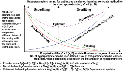
   Intuitively, according to the inductive ML from supervised data (input-output variable pairs) paradigm, either classification (where the output variable is categorical) or function regression (where the output variable is numerical) (Bishop, 1995; Cherkassky & Mulier, 1998), the well-known bias-variance cost function decomposition (bias-variance trade-off) reveals that there are two terms of cost to be jointly minimized in an expected generalization error: intuitively, the first cost term, known as bias, synonym for error rate, is monotonically non-increasing with the number of model free-parameters to be learned from data while the second cost term, known as variance, synonym for model dependence on input data, is monotonically non-decreasing with the number of model free-parameters to be learned from data, see Figure 13.

   Generalization of a either physical, statistical or hybrid (combined physical and statical) data model is the model ability to adapt properly to new, previously unseen data, drawn from the same distribution as the discrete and finite data set used to create the model (Bishop, 1995; Cherkassky & Mulier, 1998). “Generalization is the entire point of ML. Trained to solve one problem, the model attempts to utilize the patterns learned from that task to solve the same task, with slight variations. … Generalization is the act of performing tasks of the same difficulty and nature” (Ye, 2020).

   A quote of interest from Wikipedia is (Wikipedia, 2010): “The bias–variance trade-off is the property of a set of predictive inductive supervised [labeled] data learning systems [generated by changing the values of the hyperparameters, which affect the number of free-parameters to be learned-from-data], whereby models with a lower bias [error rate] in free-parameter estimation typically have a higher variance [dependence on input data] of the free-parameter estimates across samples, and vice versa. The bias-variance dilemma or problem is the conflict in trying to simultaneously minimize these two sources of error that prevent supervised data learning algorithms from generalizing beyond their training set. Hence, the bias-variance trade-off is a central problem in supervised data learning. Ideally, one wants to choose a model that accurately captures the regularities in its training data, but also generalizes well to unseen data. Unfortunately, it is typically impossible to do both simultaneously. High-variance learning methods may be able to represent their training set well, but are at risk of overfitting to noisy or unrepresentative training data. In contrast, algorithms with low variance typically produce simpler models that do not tend to overfit, but may underfit their training data, failing to capture important regularities. Models with low bias are usually more complex (e.g. higher-order regression polynomials), enabling them to represent the training set more accurately. In the process, however, they may also represent a large noise component in the training set, making their predictions less accurate – despite their added complexity. In contrast, models with higher bias tend to be relatively simple (low-order or even linear regression polynomials), but may produce lower variance predictions when applied beyond the training set”, see Figure 13.

   Although well known in the ML literature (Bishop, 1995; Cherkassky & Mulier, 1998; Geman et al., 1992; Koehrsen, 2018; Mahadevan, 2019; Sarkar, 2018; Wikipedia, 2010; Wolpert, 1996; Wolpert & Macready, 1997), the bias-variance trade-off (see Figure 13) appears largely oversighted in the ‘DCNN ⊂ DL ⊂ ML’ literature (Mahadevan, 2019; Marcus, 2018, 2020), see Figure 11. In typical ‘DL ⊃ DCNN’ applications, “[supervised, labeled, annotated] big data is never big enough” (Yuille & Liu, 2019), i.e. ‘DL ⊃ DCNN’ solutions are supervised (labeled) data hungry for training purposes by design (Lohr, 2018; Marcus, 2018, 2020). Typical ‘DL ⊃ DCNN’ models are overparameterized ANNs (Mahadevan, 2019), featuring millions of free-parameters to be learned-from-data end-to-end (Marcus, 2018, 2020).

   According to the ML literature (Bishop, 1995; Cherkassky & Mulier, 1998), the Vapnick-Chervonenkis dimension (VC-dimension) of an ANN, d_VC(ANN), is the number of training patterns the ANN at hand is able to store (memorize) exactly (Bishop, 1995; Krueger et al., 2017; Zhang, Bengio, Hardt, Recht, & Vinyals, 2017). “Only when the ANN has successfully learned a number of patterns which is much larger than its intrinsic storage capacity for random patterns (as measured by the VC-dimension) will the ANN have captured some of the structure in the data, and only then can we expect it to generalize to new data” (Bishop, 1995). In more detail, approximation d_VC(ANN) ≈ W(ANN) holds, where W(ANN) is the ANN’s number of free-parameters (e.g. weights in a multi-layer perceptron, MLP) to be learned from data (Bishop, 1995, p. 380), given that the ANN model complexity (number of degrees-of-freedom) is equal to the number of hyperparameters, to be user-defined by design, plus the number of model’s free-parameters to be learned from data (refer to this Section above). An approximate rule of thumb estimates the minimum number of training patterns, N_min, required to classify correctly a fraction (1 – ε) of new (unobserved) examples, at least equal to N_min(ANN) ≥ d_VC(ANN)/ε ≈ W(ANN)/ε, where ε is the target (testing) classification error in range (0.0, 1.0) (Bishop, 1995, p. 380).

   According to Walid Saba (Saba, 2020b), intuitively, a data memorization method is described as “knowing what” (e.g. what is the data value as outcome of a mathematical expression); it is fast and “easy”, but limited to the data that have been observed and memorized (stored). It has nothing to do with a “knowing how” (to compute a data value) method, which is not limited to the data we have seen, but requires detailed knowledge (knowing how) of the procedures. “The first method is data-driven and the second is knowledge-based. The crucial difference between ‘knowing what’ and ‘knowing how’ is that if I know how then I know what, or if I know how to compute the value of a procedure then I can always store/save the value of the outcome, but” the vice versa does not hold, e.g. “knowing the value that is stored somewhere does not mean I know how to compute it” (Saba, 2020b).

   To summarize, based on well-known ML first principles, increasingly popular ‘DL ⊃ DCNN’ models, featuring by design millions of free-parameters to be learned from data, where semantic relationship ‘DCNN ⊂ DL ⊂ ML → ANI → AGI’ = Equation (5)(5) $\text{lsquo}\mathrm{A}\mathrm{R}\mathrm{D}\subset \mathrm{E}\mathrm{O}\text{-}\mathrm{I}\mathrm{U}\subset \mathrm{C}\mathrm{V}\subset \mathrm{A}\mathrm{G}\mathrm{I}\leftarrow \mathrm{A}\mathrm{N}\mathrm{I}\leftarrow \mathrm{M}\mathrm{L}\supset \mathrm{D}\mathrm{L}\supset \mathrm{D}\mathrm{e}\mathrm{e}\mathrm{p}\mathrm{C}\mathrm{o}\mathrm{n}\mathrm{v}\mathrm{o}\mathrm{l}\mathrm{u}\mathrm{t}\mathrm{i}\mathrm{o}\mathrm{n}\mathrm{a}\mathrm{l}\mathrm{N}\mathrm{e}\mathrm{u}\mathrm{r}\mathrm{a}\mathrm{l}\mathrm{N}\mathrm{e}\mathrm{t}\mathrm{w}\mathrm{o}\mathrm{r}\mathrm{k}\left(\mathrm{D}\mathrm{C}\mathrm{N}\mathrm{N}\right)\text{rsquo}$(5) holds, are affected by two systematic drawbacks.

   • Overparameterized ‘DL ⊃ DCNN’ models are unsuitable by design for dealing with small data, either supervised (labeled, annotated, structured) or unsupervised (unlabeled) (Ball, 2021; Rowley, 2007; Stanford University, 2020; Wikipedia, 2020a).

   • According to the bias-variance trade-off (refer to references listed in this Subsection above) (see Figure 13), inductive ‘DL ⊃ DCNN’ solutions typically feature as output properties low-bias (low error rate, e.g. refer to the Vapnick-Chervonenkis dimension of an ANN, mentioned in this Subsection above) (Zhang, Bengio, Hardt, Recht, & Vinyals, 2017; Krueger et al., 2017), but high-variance (meaning high dependence on input big data, where variance is monotonically non-decreasing with the number of free-parameters). In terms of the mDMI set of OP-Q²Is proposed in the present Subsection, high dependence on input data is synonym for low transferability (Geman et al., 1992; Mahadevan, 2019; Marcus, 2018, 2020; Sarkar, 2018), low robustness to changes in input data and low scalability to changes in sensor specifications (Baraldi, 2017; Baraldi et al., 2018a, 2018b; Baraldi & Tiede, 2018a, 2018b; Wolpert, 1996; Wolpert & Macready, 1997).

   This observation agrees with the notion of “narrow idiot savant” (Langley, 2012) proposed as synonym for ‘DL ⊃ DCNN’ solutions as part-without-inheritance-of ANI = Equation (6)(6) $x0026;\text{ANI=}[\text{DCNN}\subset \text{DL}\subset \text{ML}\text{logical0OR}\text{Traditional}\text{deductive}ArtificialIntelligencex0026;(\text{static}\text{expert}\text{systems},\text{non0adaptive}\text{to}\text{data},\text{also}\text{known}\text{as}\text{Good}\text{Old0Fashioned}x0026;ArtificialIntelligence,\text{GOFAI}]$(6) (refer to Section 2). Unlike DL, to be considered as part-without-inheritance-of ANI which is part-without-inheritance-of AGI, according to Equation (5)(5) $\text{lsquo}\mathrm{A}\mathrm{R}\mathrm{D}\subset \mathrm{E}\mathrm{O}\text{-}\mathrm{I}\mathrm{U}\subset \mathrm{C}\mathrm{V}\subset \mathrm{A}\mathrm{G}\mathrm{I}\leftarrow \mathrm{A}\mathrm{N}\mathrm{I}\leftarrow \mathrm{M}\mathrm{L}\supset \mathrm{D}\mathrm{L}\supset \mathrm{D}\mathrm{e}\mathrm{e}\mathrm{p}\mathrm{C}\mathrm{o}\mathrm{n}\mathrm{v}\mathrm{o}\mathrm{l}\mathrm{u}\mathrm{t}\mathrm{i}\mathrm{o}\mathrm{n}\mathrm{a}\mathrm{l}\mathrm{N}\mathrm{e}\mathrm{u}\mathrm{r}\mathrm{a}\mathrm{l}\mathrm{N}\mathrm{e}\mathrm{t}\mathrm{w}\mathrm{o}\mathrm{r}\mathrm{k}\left(\mathrm{D}\mathrm{C}\mathrm{N}\mathrm{N}\right)\text{rsquo}$(5) = ‘DCNN ⊂ DL ⊂ ML → ANI → AGI’ (see Figure 11(a) and Figure 11(b)), AGI calls for joint (simultaneous) low bias (low error rate) and low variance (low dependence on input data), see Figure 13.

   In support of the apparently obvious (unequivocal), but not trivial observation that increasingly popular DL applications (Claire, 2019; Copeland, 2016; Krizhevsky et al., 2012) typically feature low-bias (Krueger et al., 2017; Zhang, Bengio, Hardt, Recht, & Vinyals, 2017), but high-variance by design, according to the well-known ML bias-variance first principle (see Figure 13), a renowned member of the ML community pre-dating the recent hype on DL started in 2012, Sridhar Mahadevan, wrote in 2019:

   “In agreement with the seminal work by Geman et al. (Geman et al., 1992), the essence of the ‘bias variance’ dilemma is simple to state, but it raises all sorts of profound questions that are still unresolved in brain science, Artificial Intelligence and ML. In essence, the (root mean square) error of a model in its fit to a given dataset (for function regression) can be broken into two components: the so-called ‘bias’ term [error rate], which summarizes how far a given model deviates from the best possible model and the second term is the ‘variance’ term [dependence on the input data set], which measures how far the ‘mean’ model deviates from any given learned model, if the experiment is repeated over many datasets … . As the famous saying goes, “those who ignore history are condemned to relive it”! Geman et al. point out in their summary that “to mimic substantial human behavior, such as generic object recognition in real scenes … will require complex machinery. Inferring this complexity from examples, learning it, although theoretically achievable, is, for all practical matters, not feasible: too many examples would be needed” (Geman et al., 1992). It’s remarkable how prescient this conclusion is … Is this (ongoing hype about DL) at all feasible? Geman et al. dismissed this possibility out of hand 25 years ago (Geman et al., 1992). They would be shocked to know that it has become the accepted paradigm in Artificial Intelligence and ML, and been declared a great breakthrough by every major newspaper the world over. I do think there’s a fundamental ‘bias variance’ dilemma that seems to be ignored at our peril!” (Mahadevan, 2019) (for a full quote by Sridhar Mahadevan, refer to Appendix III).

5. Computational complexity. This is a process Q²I, P-Q²I; actually, it is a cost index, to be minimized, synonym for number of elementary operations (Tsotsos, 1990), e.g. linear/ polynomial/ exponential complexity in image size.

6. Effectiveness/Accuracy. This is an outcome Q²I, O-Q²I, to be maximized, inversely related to the bias term (error rate) to be minimized in the bias-variance cost function, see Figure 13. For example, in image interpretation (classification) tasks: (a) thematic Q²Is (T-Q²Is) and (b) spatial Q²Is (S-Q²Is), where S-Q²Is estimate the 2D spatial distribution of T-Q²Is, can be designed to be statistically independent. In compliance with the intergovernmental GEO-CEOS QA4EO Val guidelines (GEO-CEOS – Group on Earth Observations and Committee on Earth Observation Satellites, 2010), T-Q²Is and S-Q²Is must be provided with a degree of uncertainty in measurement, ±δ (Baraldi, 2017; Baraldi et al., 2014; ESA, 2017a; GEO-CEOS – Group on Earth Observations and Committee on Earth Observation Satellites, 2010; Holdgraf, 2013; JCGM – Joint Committee for Guides in Metrology, 2008, 2012; Lunetta & Elvidge, 1999).

   Unfortunately, the large majority of works published in the RS literature presents OP-Q²I estimates, such as statistical estimates of T-Q²Is, provided with no degree of uncertainty in measurement, ±δ (Lunetta & Elvidge, 1999). It is important to stress that OP-Q²Is published in the RS literature featuring no uncertainty estimate, ±δ, are in contrast with the principles of statistics (GEO-CEOS – Group on Earth Observations and Committee on Earth Observation Satellites, 2010; Holdgraf, 2013; JCGM – Joint Committee for Guides in Metrology, 2008, 2012; Lunetta & Elvidge, 1999), i.e. they do not feature any statistical meaning (Baraldi, 2017; Baraldi et al., 2014; Baraldi & Tiede, 2018a, 2018b; Holdgraf, 2013), and they are in contrast with intergovernmental GEO-CEOS QA4EO Val requirements (GEO-CEOS – Group on Earth Observations and Committee on Earth Observation Satellites, 2010). If this observation holds true as premise, by deduction rule of inference (modus ponens, forward chaining, refer to the farther Subsection 3.3.4), then another fact holds true as consequence: since large portions of OP-Q²Is published in the RS literature feature no degree of uncertainty in measurement, ±δ, in disagreement with intergovernmental GEO-CEOS QA4EO Val requirements (GEO-CEOS – Group on Earth Observations and Committee on Earth Observation Satellites, 2010), then the statistical quality of a large portion of outcomes and/or processes published in the RS literature remains unknown to date.

7. Efficiency. This is a process Q²I, P-Q²I, to be maximized. For example, it comprises: (a) computation time (cost index, to be minimized), monotonically non-decreasing with computational complexity and energy consumption (Hao, 2019; Strubell et al., 2019; Wolski, 2020a, 2020b), and (b) run-time memory occupation (cost index, to be minimized).

8. Robustness/Reliability (vice versa, Sensitivity, to be minimized) to changes in input data. It is a process Q²I, P-Q²I, to be maximized, such as robustness to changes in EO big data acquired at large spatial and/or temporal extent (no toy problem). It is related to other P-Q²Is such as interoperability and transferability, e.g. AGI aims at low bias (low error rate) together with low variance (meaning low dependence on input data, high robustness/ interoperability/ transferability), see Figure 11.

9. Robustness/Reliability (vice versa, Sensitivity, to be minimized) to changes in input hyperparameters. This is a process Q²I, P-Q²I, to be maximized. As mentioned above, to be user-defined based on heuristics (trial-and-error), system hyperparameters are equivalent to a priori knowledge to be encoded by design. For example, in popular ‘DCNN ⊂ DL’ algorithms (Cimpoi et al., 2014; Krizhevsky et al., 2012), typical hyperparameters are the number of layers, the number of features per layer, the spatial filter size, the spatial filter stride, the spatial pooling size, the spatial pooling stride, etc. Worth mentioning, it is a general rule that “proper feature engineering will have a much larger impact on model performance than even the most extensive hyperparameter tuning. It is the law of diminishing returns applied to machine learning: feature engineering gets you most of the way there, and hyperparameter tuning generally only provides a small benefit. This demonstrates a fundamental aspect of machine learning: it is always a game of trade-offs. We constantly have to balance accuracy vs interpretability, bias vs variance, accuracy vs run time, and so on” (Koehrsen, 2018), see Figure 11.

10. Scalability to changes in sensor specifications and/or user requirements, synonym for Reusability/ Maintainability/ Transferability. This is a process Q²I, P-Q²I, to be maximized. For example, to comply with human vision, where panchromatic (achromatic) and chromatic vision are nearly as effective in scene-from-image reconstruction and understanding tasks (Baraldi, 2017; Baraldi & Tiede, 2018a, 2018b), a CV system to be considered scalable is required to perform nearly as well when input with either panchromatic or chromatic imagery (refer to the farther Subsection 4.1).

11. Interpretability/ Traceability/ Accountability/ Explainability of the model/solution (Koehrsen, 2018; Lukianoff, 2019; Sweeney, 2018a). This is a process Q²I, P-Q²I, to be maximized. In contrast with “the black box problem”, typically affecting ANNs (Baraldi & Tiede, 2018a, 2018b; Lukianoff, 2019; Marcus, 2018, 2020), including inductive DCNNs, learned from data end-to-end (Cimpoi et al., 2014; Krizhevsky et al., 2012), see Figure 14.

    Figure 14. Adapted from (Koehrsen, 2018). The so-called “black box problem” closes in on machine learning (ML)-from-data algorithms in general. In artificial neural networks (ANNs), typically based on the McCulloch and Pitts (MCP) neuron model, conceived almost 80 years ago as a simplified neurophysiological version of biological neurons (McCulloch & Pitts, 1943), or its improved recent versions (Cimpoi et al., 2014; Krizhevsky et al., 2012), in compliance with the mind-brain problem (Hassabis et al., 2017; Hoffman, 2008; Serra & Zanarini, 1990; Westphal, 2016), the difficulty for the system to provide a suitable explanation for how it arrived at an answer is referred to as “the black box problem”, which affects how an ANN can hit the point of reproducibility or at least traceability/interpretability (Koehrsen, 2018; Lukianoff, 2019). This chart shows “a (highly unscientific) version of the accuracy vs interpretability trade-off, to highlight a fundamental aspect of ML: it is always a game of trade-offs. We constantly have to balance accuracy vs interpretability, bias vs variance, accuracy vs run time, and so on” (Koehrsen, 2018), also refer to Figure 13.

    

12. Timeliness. This is a process Q²I, P-Q²I; actually, it is a cost index, to be minimized. Timeliness is defined as the time span from data acquisition to output product generation. It increases monotonically with manpower and computing power. For example, timeliness monotonically increases with the time required by ML systems for, first, training and, second, executing. Unfortunately, to date, in the ML literature, training time is typically oversighted in ANN quality assessment and inter-comparison (Hao, 2019).

13. Costs. This is either an outcome Q²I, O-Q²I, and/or a process Q²I, P-Q²I; actually it is a cost index, to be minimized. It is monotonically increasing with manpower (including manpower required to collect training data, if any) and computing power, e.g. energy consumption, typically “high” in DCNN applications to be considered unsustainable (Hao, 2019; Strubell et al., 2019; Wolski, 2020a, 2020b).

14. Value. This is either an outcome Q²I, O-Q²I, and/or a process Q²I, P-Q²I, to be maximized. For example, semantic information value of the outcome, economic value of output products or services, etc.

According to Section 2, an information processing system is defined in operational mode if and only if it scores (fuzzy) “high” in each Q²I belonging to an mDMI set of OP-Q²Is, to be jointly maximized in agreement with the Pareto formal analysis of inherently ill-posed multi-objective optimization problems (Hadamard, 1902). This definition agrees with common sense. Intuitively, no automobile can be expected to be considered in “operational mode”, to be sold in a competitive free-market, if it looks ok, it runs fast enough, it handles the road well, but it costs a lot of money or, vice versa, if it looks ok, it runs fast enough, its cost is reasonable, but whose handling is rather bad. It means that if a single Q²I in the mDMI set of community-agreed OP-Q²Is scores (fuzzy) “low” then it suffices for an information processing system not to be considered in operational mode; for example, a ‘CV ⊃ EO-IU’ system scoring low in degree of automation or low in transferability (due to high-variance, see Figure 13) may be considered of no potential interest for a worldwide market of unskilled end-users of space technology, in a new notion of Space Economy 4.0, see Figure 10.

3.2. The Marr five levels of system understanding, applicable to ‘AGI ⊃ CV ⊃ EO-IU ⊃ ARD’ systems research and development

According to Section 2, instantiation of a community-agreed mDMI set of OP-Q²Is (such as that proposed in Subsection 3.1 above) is necessary-but-not-sufficient precondition to the quantitative quality assessment of any information processing system, investigated at the Marr five levels of system understanding.

According to the Marr seminal work (Marr, 1982), levels of understanding (levels of abstraction) of an information processing system, such as an ‘AGI ⊃ CV ⊃ EO-IU ⊃ ARD’ system, are proposed as follows (Baraldi, 2017; Baraldi et al., 2018a, 2018b; Baraldi & Tiede, 2018a, 2018b; Marr, 1982; Quinlan, 2012; Sonka et al., 1994).

• Marr level of system understanding 1-of-5: Outcome and process requirements specification, including degree of automation, accuracy, efficiency, etc. for example, refer to the mDMI set of OP-Q²Is instantiated in Subsection 3.1. Outcome and process requirements are typically expressed in user-speak (natural language), to be translated into techno-speak in a so-called statement of external functionality (Brinkworth, 1992).

• Marr level of system understanding 2-of-5: Information and/or knowledge representation, in compliance with the increasingly popular DIKW hierarchical conceptualization (refer to references listed in Section 2), see Figure 12. For example, in the cognitive task of biological vision, where achromatic and chromatic vision are nearly as effective (refer to Subsection 3.1), 2D spatial topological and non-topological information components typically dominate colorimetric information (refer to the farther Subsection 4.1).

• Marr level of system understanding 3-of-5: System design (architecture), provided with a data/information flow and a control flow (Page-Jones, 1988). For example, structured system design is required to comply with the engineering criteria of modularity, hierarchy and regularity, considered neither necessary nor sufficient, but highly recommended for system scalability (Lipson, 2007; Page-Jones, 1988). The structured system design criterion of regularity coincides with the principle of reusability adopted by the popular FAIR guiding principles for scientific data (product and process) management (GO FAIR – International Support and Coordination Office, 2021; Wilkinson et al., 2016), see Table 1.

• Marr level of system understanding 4-of-5: Algorithm, to be selected among existing algorithmic solutions or developed from scratch for each module in a structured system design.

• Marr level of system understanding 5-of-5: Implementation, to be selected among existing solutions or accomplished from scratch for each selected algorithm.

Noteworthy, among the Marr five levels of system understanding, the three more abstract levels, namely, outcome and process requirements specification, information/knowledge representation and system design, are typically considered the linchpin for success of an information processing system, rather than algorithm and implementation (Baraldi, 2017; Baraldi et al., 2018a, 2018b; Baraldi & Tiede, 2018a, 2018b; Marr, 1982; Quinlan, 2012; Sonka et al., 1994). Although based on commonsense knowledge (refer to references listed in Section 2), this observation (true-fact) is oversighted in large portions of the RS and CV literature, where ‘CV ⊃ EO-IU’ system analysis, assessment and inter-comparison are typically focused on algorithm and implementation, e.g. refer to (Foga et al., 2017) and (Ghosh & Kaabouch, 2014) as negative examples not to be imitated in CV systems inter-comparison.

3.3. Augmented DIKW hierarchical conceptualization, applicable to ‘AGI ⊃ CV ⊃ EO-IU ⊃ ARD’ systems research and development

Following the well-known DIKW hierarchical conceptualization (refer to references listed in Section 2) (see Figure 12), where information is typically defined in terms of data, knowledge in terms of information and wisdom in terms of knowledge, more notions of interest are critically reviewed hereafter.

Pertaining to the multi-disciplinary domain of cognitive science (see Figure 11), philosophical hermeneutics (Capurro & Hjørland, 2003; Dreyfus, 1965, 1991, 1992) provides a fundamental contribution in the formalization of the two notions of data and information, corresponding to the first two (shallowest) levels of conceptualization in the DIKW pyramid, whose discrimination is of paramount importance in a so-called era of ICT, where convergence of audiovisual and telephone (communication) networks with computer (information) networks through a single cabling or link system is pursued (Wikipedia, 2009).

3.3.1. Data as numerical variables, either continuous or discrete, and data-derived information as categorical variables, discrete and finite, either ordinal or non-ordinal

In a taxonomy of levels of measurement proposed in (Baraldi, 2017; Wikipedia, 2011, 2012), data is synonym for sensory data, observables or true-facts. Sensory data are numerical variables, either uncalibrated (provided with no physical meaning, therefore dimensionless) or calibrated (provided with a physical meaning, a physical unit of measure and a physical range of change) (Baraldi, 2009; GEO-CEOS – Group on Earth Observations and Committee on Earth Observation Satellites, 2010; Schaepman-Strub et al., 2006; Shuai et al., 2020). Sensory data-derived variables are either numerical or categorical/nominal variables. Numerical variables are either continuous (uncountable) or discrete (countable, but potentially infinite). Numerical variables are always ordinal variables. Instances of an ordinal variable can be ordered and the distance between two variable instantiations is known. Categorical/nominal variables, belonging to a discrete and finite vocabulary of categories (nouns), can be discriminated as follows.

• Categorical (discrete and finite) ordinal variables. It holds if the categorical variable has a clear ordering, such as fuzzy (qualitative) data sets, e.g. fuzzy sets low, medium and high of a numerical variable (Zadeh, 1965). In a (2D) image-plane, field-objects (Couclelis, 2010; Goodchild et al., 2007) are examples of categorical ordinal variables, e.g. a DEM’s elevation dimension is discretized into three fuzzy sets “high”, “medium” or “low”.

• Categorical (discrete and finite) non-ordinal variables. They can be distinguished/discretized into three (sub)categories.

  • Semantic (symbolic) variables, belonging to a discrete and finite vocabulary of classes (entities) of real-world objects/continuants (refer to references listed in Section 2). A vocabulary of classes/entities of real-world objects is part-of a 7D (refer to Section 2) mental model of the 4D geospace-time real-world, also known as conceptual world model or world ontology (refer to references listed in Section 2), see Figure 3. In a (2D) image-plane, so-called geo-objects (refer to Section 2), popular in GIScience (refer to references listed in Section 2), are discrete and finite instances of semantic variables in the 4D geospace-time world-domain projected onto an image-plane by an imaging sensor (refer to the farther Subsection 4.1).

  • Semi-symbolic, latent/ hidden/ hypothetical categorical variable. In statistics, the popular concept of latent/hidden categorical variable was introduced to fill the information gap from input numerical observables, e.g. subsymbolic sensory data such as color values in a color space, to an output categorical variable, such as a discrete and finite vocabulary of target LC classes in the mental model of the physical world (Baraldi, 2017; Baraldi & Tiede, 2018a, 2018b; Matsuyama & Hwang, 1990), see Figure 3. Latent/hidden variables are categorical variables not directly measured, but inferred from lower level variables. “The terms hypothetical variable or hypothetical construct may be used when latent variables correspond to abstract concepts, like perceptual categories or discrete mental states” (Shotton et al., 2009; Wikipedia, 2015). Hence, to fill the semantic gap from input subsymbolic sensory data to an output categorical variable of symbolic quality, such as a LC class taxonomy (see Figure 3), a hypothetical categorical variable, such as a discrete and finite vocabulary of basic color (BC) names (Benavente et al., 2008; Berlin & Kay, 1969; Griffin, 2006; Parraga et al., 2009), is considered to be of “semi-symbolic” quality, i.e. its semantic value is superior to the zero semantics of sensory data, but inferior to the symbolic quality of output LC classes (Baraldi, 2017; Baraldi & Tiede, 2018a, 2018b), see Figure 15.

    Figure 15. Example of latent/hidden variable as a discrete and finite vocabulary of basic color (BC) names (Baraldi & Tiede, 2018a, 2018b; berlin & Kay, 1969; Griffin, 2006). This graphical model of color naming is adapted from (Shotton, Winn, Rother, & Criminisi, 2009; Wikipedia, 2015). Let us consider z as a (subsymbolic) numerical variable, such as multi-spectral (MS) color values of a population of spatial units belonging to a (2D) image-plane, where spatial units can be either (0D) pixel, (1D) line or (2D) polygon (OGC – Open Geospatial Consortium Inc, 2015), with vector data z ∈ ℜ^MS, where ℜ^MS represents a multi-spectral (MS) data space, while c represents a categorical variable of symbolic classes in the 4D geospace-time scene-domain, pertaining to the physical real-world, with c = 1, …, ObjectClassLegendCardinality. (a) According to Bayesian theory, posterior probability $\mathrm{p}\left(\mathrm{c}|\mathrm{z}\right)\text{prop}\mathrm{p}\left(\mathrm{z}|\mathrm{c}\right)\mathrm{p}\left(\mathrm{c}\right)=\mathrm{p}\left(\mathrm{c}\right)\sum _{\mathrm{k}\text{-}\mathrm{t}\mathrm{h}\mathrm{C}\mathrm{o}\mathrm{l}\mathrm{o}\mathrm{r}\mathrm{N}\mathrm{a}\mathrm{m}\mathrm{e},\mathrm{k}=1}^{\mathrm{C}\mathrm{o}\mathrm{l}\mathrm{o}\mathrm{r}\mathrm{V}\mathrm{o}\mathrm{c}\mathrm{a}\mathrm{b}\mathrm{u}\mathrm{l}\mathrm{a}\mathrm{r}\mathrm{y}\mathrm{C}\mathrm{a}\mathrm{r}\mathrm{d}\mathrm{i}\mathrm{n}\mathrm{a}\mathrm{l}\mathrm{i}\mathrm{t}\mathrm{y}}\mathrm{p}\left(\mathrm{z}|\mathrm{k}\right)\mathrm{p}\left(\mathrm{k}|\mathrm{c}\right)$, where color names ks, equivalent to color (hyper)polyhedra (Benavente et al., 2008; Griffin, 2006; Parraga et al., 2009) in a numerical color (hyper)space ℜ^MS, provide a partition of the domain of change, ℜ^MS, of numerical variable z (refer to the farther Figure 29). (b) For discriminative inference, the arrows in the graphical model are reversed using Bayes rule. Hence, a vocabulary of color names, physically equivalent to a partition of a numerical color space ℜ^MS into color name-specific hyperpolyhedra, is conceptually equivalent to a latent/ hidden/ hypothetical variable linking observables (subsymbolic sensory data) in the real world, specifically, color values, to a categorical variable of semantic (symbolic) quality in the mental (conceptual) model of the physical world (world ontology, world model) (Baraldi, 2017; Baraldi & Tiede, 2018a, 2018b; Matsuyama & Hwang, 1990).

    

  • Subsymbolic categorical variables, e.g. unlabeled data cluster/category 1, unlabeled data cluster/category 2, etc., in unsupervised (unlabeled) data clustering tasks (Baraldi & Alpaydin, 2002a, 2002b; Bishop, 1995; Cherkassky & Mulier, 1998; Fritzke, 1997).

To summarize, symbolic (categorical and semantic) variables, such as classes of real-world continuants belonging to a mental (conceptual) model of the world (world model, world ontology) (refer to Section 2), are always non-ordinal categorical variables. The vice versa does not hold, i.e. not all categorical variables (e.g. unlabeled data clusters) are provided with semantics.

3.3.2. Calibrated and uncalibrated sensory data, with special emphasis on EO data in the RS meta-science domain

The two subcategories of sensory data/ observables/ true-facts, specifically, numerical variables either uncalibrated or calibrated, deserve further comments, with special emphasis on their difference in ease of use and degree of informativeness (the condition of being informative).

Uncalibrated numerical variables are always dimensionless, i.e. they are pure numbers, and lack any physical meaning. Calibrated numerical variables are provided with a physical meaning, a physical unit of measure (eventually, dimensionless) and a physical range of change. Hence, calibrated sensory data, provided with a physical meaning, are better behaved/conditioned and better understood than uncalibrated sensory data (Baraldi, 2009; Pacifici et al., 2014).

Intuitively, what would happen to our human lives if the artificial physical sensors we rely upon, say, our car’s speedometer, the thermometer in our oven, etc., were uncalibrated or poorly calibrated? Undoubtedly, when dealing with uncalibrated or poorly calibrated sensory data, our human lives in the physical world would become very difficult/ ill-posed/ poorly conditioned. Human decisions based on poorly behaved and poorly understood uncalibrated sensory data would be undertaken according to heuristic criteria, synonym for trial-and-error solutions, equivalent to ad-hoc “narrow” data- user- and application-specific strategies affected by low transferability (to different application domains) and low reusability (in the same domain of applications). For example, when driving a car whose speedometer is uncalibrated, a driver may figure that the uncalibrated speedometer’s value ought to be divided by two to drive safely. Whenever the same driver changes the car to drive, no such heuristics is likely to be ever reused as a priori knowledge, available in addition to sensory data.

Pertaining to the realm of commonsense knowledge, shared by all human beings as community-agreed knowledge baseline (refer to references listed in Section 2), an obvious observation is that, to live successfully in a physical world, no human being would ever choose to be provided with uncalibrated physical sensors over calibrated physical sensors. Quite enigmatically, this intuitive baseline knowledge is ignored or oversighted in the domains of the RS and ML meta-sciences, as explained below.

In technical terms, since calibrated sensory data are better behaved and better understood than uncalibrated sensory data, then the former are more suitable for pursuing the interoperability and reusability criteria of the standard FAIR guiding principles for scholarly/scientific digital data and non-data (e.g. analytical pipelines) research objects management (GO FAIR – International Support and Coordination Office, 2021; Wilkinson et al., 2016), in agreement with the criterion of regularity/reusability adopted by the structured processing system design principles of modularity (where a problem is divided into subproblems, easier to be coped with), hierarchy (to benefit from inter-problem semantic relationships part-without-inheritance-of and subset-with-inheritance-of, if any) and regularity/reusability (Lipson, 2007), considered neither necessary nor sufficient, but highly recommended for system scalability (Page-Jones, 1988) (refer to Section 2).

In more detail, a first reason of technical relevance of calibrated sensory data over uncalibrated data is that, in general, uncalibrated data, provided with no physical meaning, are eligible for statistical data analysis exclusively, encompassing inductive/ bottom-up/ statistical (data-driven) inference systems, such as ‘ML ⊃ DL ⊃ DCNN’ algorithms (Bishop, 1995; Cherkassky & Mulier, 1998).

On the contrary, calibrated data are provided with a physical meaning, a physical unit of measure and a physical range of change. Hence, they can be input to either:

• Inductive/ bottom-up/ statistical (data-driven) inference systems, such as ‘ML ⊃ DL ⊃ DCNN’ algorithms (Bishop, 1995; Cherkassky & Mulier, 1998; Salmon, 1963). In general, statistical model-based systems can be input with either uncalibrated or calibrated data. If input with calibrated data, which are better behaved/conditioned than uncalibrated data, then statistical model-based systems typically gain in accuracy, robustness, transferability and scalability (refer to Subsection 3.1).

  Inductive ML-from-data inference is inherently ill-posed in the Hadamard sense (Hadamard, 1902) and requires a priori knowledge in addition to data to become better conditioned for numerical solution (Bishop, 1995; Cherkassky & Mulier, 1998, p. 21). As a consequence of their inherent ill-posedness, inductive ML-from-data algorithms are typically semi-automatic (where system hyperameters must be user-defined based on heuristics, refer to Subsection 3.1) and site-specific (data-dependent) (Liang, 2004) (refer to the bias-variance trade-off in Subsection 3.1).

  In general, “No Free Lunch” theorems have shown that inductive learning-from-data algorithms cannot be universally good (Wolpert, 1996; Wolpert & Macready, 1997), i.e. there’s no one-size-fits-all inductive learning-from-data algorithm that will help you solve every problem and tackle every dataset based on a finite data sample. In other words, “finite-sample generalization without assumptions on function classes is impossible” (Schölkopf et al., 2021).

And/or

• Deductive/ top-down/ physical model-based/ prior knowledge-based inference algorithms such as expert systems/decision support systems (Laurini & Thompson, 1992; Sonka et al., 1994), consisting of prior knowledge-based if-then decision rules, non-adaptive to data (static decision trees). Physical model-based information processing systems cannot work if input data are not provided with a physical meaning, i.e. they require calibrated data as input.

  Deductive inference is static (non-adaptive to data) and typically lacks flexibility to transform ever-varying sensory data (sensations) into stable percepts (concepts) in a stable/hard-to-vary (Sweeney, 2018a), but plastic (adaptive, self-organizing, capable of incremental learning and forgetting to model non-stationary data distributions) (Baraldi & Alpaydin, 2002a, 2002b; Fritzke, 1997; Langley, 2012; Mermillod et al., 2013; Wolski, 2020a, 2020b) conceptual/ mental/ perceptual model of the 4D geospace-time physical world (Baraldi, 2017; Baraldi & Tiede, 2018a, 2018b; Hassabis et al., 2017; Laurini & Thompson, 1992; Liang, 2004; Mindfire Foundation, 2018; Nagao & Matsuyama, 1980; Wolski, 2020a, 2020b).

And/or

• Hybrid (combined) deductive/top-down/ physical model-driven and inductive/ bottom-up/ statistical data-driven inference systems (Baraldi, 2017; Baraldi & Tiede, 2018a, 2018b; Bishop, 1995; Cherkassky & Mulier, 1998; Chomsky, 1957; Expert.ai, 2020; Hassabis et al., 2017; Laurini & Thompson, 1992; Liang, 2004; Marcus, 2018, 2020; Matsuyama & Hwang, 1990; Mindfire Foundation, 2018; Nagao & Matsuyama, 1980; Parisi, 1991; Piaget, 1970; Sonka et al., 1994; Sweeney, 2018b; Thompson, 2018; Zador, 2019).

  Hybrid inference combines deductive with inductive inference, “to take advantage of each and overcome their shortcomings” (Liang, 2004).

  A hybrid (combined deductive and inductive) inference paradigm agrees with Noam Chomsky, who argued that humans are born wired to learn from experience, programmed to master language and interpret the physical world (Chomsky, 1957; Thompson, 2018) and with Gary Marcus who argued that, to overcome its current limitations, what DL needs is a boost – rules that supplement or are built in to help it reason about the physical world (Marcus, 2018, 2020; Thompson, 2018). It also complies with the Marr seminal work on vision (Marr, 1982), where Marr’s computational constraints, reflecting properties of the world embodied through evolution into the human visual system (Quinlan, 2012), are encoded by design. Last, but not least, it agrees with biological cognitive systems, where “there is never an absolute beginning” (Baraldi, 2017; Parisi, 1991; Piaget, 1970; Zador, 2019).

  Since a physical model-based subsystem belonging to a hybrid inference system cannot work if input data are not provided with a physical meaning, then hybrid inference systems require at least a portion of the input data to be (e.g. radiometrically) calibrated.

In line with the aforementioned commonsense knowledge (refer to references listed in Section 2), in the RS meta-science domain (Couclelis, 2012) (see Figure 11(a)), to better cope with the six Vs of EO big data, namely, volume, variety, veracity, velocity, volatility and value (Metternicht et al., 2020), radiometric Cal of EO sensory data is regarded as a well-known “prerequisite for physical model-based analysis of airborne and satellite sensor measurements in the optical domain” (Schaepman-Strub et al., 2006). In more detail, radiometric Cal of EO sensory data is considered mandatory by the standard intergovernmental GEO-CEOS QA4EO Cal/Val guidelines (refer to references listed in Section 2), whose overarching goal is systematic transformation of EO big data into operational, timely and comprehensive EO data-derived VAPS, in agreement with the GEO visionary goal of a GEOSS implementation plan for years 2005–2015 (EC – European Commission and GEO – Group on Earth Observations, 2014; GEO – Group on Earth Observations, 2005, 2019; Mavridis, 2011), unaccomplished to date and revised by a GEO’s second implementation plan for years 2016–2025 of a new GEOSS, regarded as expert EO data-derived information and knowledge system (GEO – Group on Earth Observations, 2015; Nativi et al., 2015, 2020; Santoro et al., 2017), see Figure 1.

In the RS common practice, radiometric Cal (refer to references listed in Section 2) is the process of transforming EO sensory data, such as EO optical imagery, typically encoded as non-negative dimensionless digital numbers (DNs, with DN ≥ 0) provided with no physical meaning at EO Level 0, into a physical radiometric variable, provided with a physical meaning, a community-agreed radiometric unit of measure and range of change (Baraldi, 2009, 2017; Baraldi et al., 2018a, 2018b; Baraldi & Tiede, 2018a, 2018b; DigitalGlobe, 2017; EC – European Commission, 2020; GEO-CEOS – Group on Earth Observations and Committee on Earth Observation Satellites, 2010; Malenovsky et al., 2007; Pacifici et al., 2014; Schaepman-Strub et al., 2006; Shuai et al., 2020), such as top-of-atmosphere radiance (TOARD) values, with TOARD ≥ 0, top-of-atmosphere reflectance (TOARF) values belonging to the physical domain of change [0.0, 1.0], surface reflectance (SURF) values in the physical range of change [0.0, 1.0] and surface albedo values in the physical range [0.0, 1.0]. Noteworthy, surface albedo is included (referred to as albedo) in the list of terrestrial ECVs defined by the WCO (see Table 2), which complies with requirements of the GEO second implementation plan for years 2016–2025 of a new GEOSS, regarded as expert EO data-derived information and knowledge system (refer to references listed in Section 2) (see Figure 1), in agreement with the well-known DIKW hierarchical conceptualization where, typically, information is defined in terms of data, knowledge in terms of information and wisdom in terms of knowledge, see Figure 12.

When EO optical sensory data, acquired as dimensionless DN ≥ 0 at EO Level 0, are radiometrically calibrated into TOARF values ∈ [0.0, 1.0] at EO Level 1, SURF values ∈ [0.0, 1.0] at EO Level 2/(current, existing) ARD and surface albedo values ∈ [0.0, 1.0] at, say, EO Level 3/next generation ARD where, for example, terrestrial ECVs, including surface albedo (see Table 2), are systematically estimated as standard information products required by end-users in the framework of a new GEOSS implementation plan for years 2016–2025 (refer to references listed in Section 2) (see Figure 1), an intuitive set relation

(8) $\begin{array}{rl}& \text{lsquo}\mathrm{D}\mathrm{N}\mathrm{s}\ge 0\mathrm{a}\mathrm{t}\mathrm{E}\mathrm{O}\mathrm{L}\mathrm{e}\mathrm{v}\mathrm{e}\mathrm{l}0\supseteq \mathrm{T}\mathrm{O}\mathrm{A}\mathrm{R}\mathrm{F}\in \left[0.0,1.0\right]\mathrm{a}\mathrm{t}\mathrm{E}\mathrm{O}\mathrm{L}\mathrm{e}\mathrm{v}\mathrm{e}\mathrm{l}1\supseteq \mathrm{S}\mathrm{U}\mathrm{R}\mathrm{F}\in \left[0.0,1.0\right]\\ & \mathrm{a}\mathrm{t}\mathrm{E}\mathrm{O}\mathrm{L}\mathrm{e}\mathrm{v}\mathrm{e}\mathrm{l}2/\left(\mathrm{c}\mathrm{u}\mathrm{r}\mathrm{r}\mathrm{e}\mathrm{n}\mathrm{t}\right)\mathrm{A}\mathrm{R}\mathrm{D}\supseteq \mathrm{S}\mathrm{u}\mathrm{r}\mathrm{f}\mathrm{a}\mathrm{c}\mathrm{e}\mathrm{a}\mathrm{l}\mathrm{b}\mathrm{e}\mathrm{d}\mathrm{o}\in \left[0.0,1.0\right]\mathrm{a}\mathrm{t},\mathrm{s}\mathrm{a}\mathrm{y},\mathrm{E}\mathrm{O}\mathrm{L}\mathrm{e}\mathrm{v}\mathrm{e}\mathrm{l}3/\mathrm{n}\mathrm{e}\mathrm{x}\mathrm{t}\\ & \mathrm{g}\mathrm{e}\mathrm{n}\mathrm{e}\mathrm{r}\mathrm{a}\mathrm{t}\mathrm{i}\mathrm{o}\mathrm{n}\mathrm{A}\mathrm{R}\mathrm{D}\text{rsquo}& (8)\end{array}$(8)

holds true. Equation (8)(8) $\begin{array}{rl}& \text{lsquo}\mathrm{D}\mathrm{N}\mathrm{s}\ge 0\mathrm{a}\mathrm{t}\mathrm{E}\mathrm{O}\mathrm{L}\mathrm{e}\mathrm{v}\mathrm{e}\mathrm{l}0\supseteq \mathrm{T}\mathrm{O}\mathrm{A}\mathrm{R}\mathrm{F}\in \left[0.0,1.0\right]\mathrm{a}\mathrm{t}\mathrm{E}\mathrm{O}\mathrm{L}\mathrm{e}\mathrm{v}\mathrm{e}\mathrm{l}1\supseteq \mathrm{S}\mathrm{U}\mathrm{R}\mathrm{F}\in \left[0.0,1.0\right]\\ & \mathrm{a}\mathrm{t}\mathrm{E}\mathrm{O}\mathrm{L}\mathrm{e}\mathrm{v}\mathrm{e}\mathrm{l}2/\left(\mathrm{c}\mathrm{u}\mathrm{r}\mathrm{r}\mathrm{e}\mathrm{n}\mathrm{t}\right)\mathrm{A}\mathrm{R}\mathrm{D}\supseteq \mathrm{S}\mathrm{u}\mathrm{r}\mathrm{f}\mathrm{a}\mathrm{c}\mathrm{e}\mathrm{a}\mathrm{l}\mathrm{b}\mathrm{e}\mathrm{d}\mathrm{o}\in \left[0.0,1.0\right]\mathrm{a}\mathrm{t},\mathrm{s}\mathrm{a}\mathrm{y},\mathrm{E}\mathrm{O}\mathrm{L}\mathrm{e}\mathrm{v}\mathrm{e}\mathrm{l}3/\mathrm{n}\mathrm{e}\mathrm{x}\mathrm{t}\\ & \mathrm{g}\mathrm{e}\mathrm{n}\mathrm{e}\mathrm{r}\mathrm{a}\mathrm{t}\mathrm{i}\mathrm{o}\mathrm{n}\mathrm{A}\mathrm{R}\mathrm{D}\text{rsquo}& (8)\end{array}$(8) accounts for the following two qualitative relationships (Baraldi, 2017, 2019a; Baraldi & Boschetti, 2012a, 2012b; Baraldi et al., 2014, 2010a, 2010b, 2010, 2018a, 2018b, 2006; Baraldi & Tiede, 2018a, 2018b; Bishop & Colby, 2002; Chavez, 1988; DLR – Deutsches Zentrum für Luft-und Raumfahrt e.V. and VEGA Technologies, 2011; ESA – European Space Agency, 2015; Irish, 2000; Liang, 2004; Lillesand & Kiefer, 1979; Pacifici, 2016; Pacifici et al., 2014; Swain & Davis, 1978) (also refer to Figure 30 below in this text).

(9) $\begin{array}{rl}& \text{lsquo}\mathrm{T}\mathrm{O}\mathrm{A}\mathrm{R}\mathrm{F}\approx \mathrm{S}\mathrm{U}\mathrm{R}\mathrm{F}\pm \mathrm{r}\mathrm{a}\mathrm{d}\mathrm{i}\mathrm{o}\mathrm{m}\mathrm{e}\mathrm{t}\mathrm{r}\mathrm{i}\mathrm{c}\mathrm{n}\mathrm{o}\mathrm{i}\mathrm{s}\mathrm{e}\mathrm{v}\mathrm{a}\mathrm{r}\mathrm{i}\mathrm{a}\mathrm{t}\mathrm{i}\mathrm{o}\mathrm{n}1,\mathrm{d}\mathrm{u}\mathrm{e}\mathrm{t}\mathrm{o}\mathrm{a}\mathrm{t}\mathrm{m}\mathrm{o}\mathrm{s}\mathrm{p}\mathrm{h}\mathrm{e}\mathrm{r}\mathrm{i}\mathrm{c}\mathrm{e}\mathrm{f}\mathrm{f}\mathrm{e}\mathrm{c}\mathrm{t}\mathrm{s},\\ & \pm \mathrm{r}\mathrm{a}\mathrm{d}\mathrm{i}\mathrm{o}\mathrm{m}\mathrm{e}\mathrm{t}\mathrm{r}\mathrm{i}\mathrm{c}\mathrm{n}\mathrm{o}\mathrm{i}\mathrm{s}\mathrm{e}\mathrm{v}\mathrm{a}\mathrm{r}\mathrm{i}\mathrm{a}\mathrm{t}\mathrm{i}\mathrm{o}\mathrm{n}2,\mathrm{d}\mathrm{u}\mathrm{e}\mathrm{t}\mathrm{o}\mathrm{t}\mathrm{o}\mathrm{p}\mathrm{o}\mathrm{g}\mathrm{r}\mathrm{a}\mathrm{p}\mathrm{h}\mathrm{i}\mathrm{c}\mathrm{e}\mathrm{f}\mathrm{f}\mathrm{e}\mathrm{c}\mathrm{t}\mathrm{s},\\ & \pm \mathrm{r}\mathrm{a}\mathrm{d}\mathrm{i}\mathrm{o}\mathrm{m}\mathrm{e}\mathrm{t}\mathrm{r}\mathrm{i}\mathrm{c}\mathrm{n}\mathrm{o}\mathrm{i}\mathrm{s}\mathrm{e}\mathrm{v}\mathrm{a}\mathrm{r}\mathrm{i}\mathrm{a}\mathrm{t}\mathrm{i}\mathrm{o}\mathrm{n}3,\mathrm{d}\mathrm{u}\mathrm{e}\mathrm{t}\mathrm{o}\mathrm{a}\mathrm{d}\mathrm{j}\mathrm{a}\mathrm{c}\mathrm{e}\mathrm{n}\mathrm{c}\mathrm{y}\mathrm{e}\mathrm{f}\mathrm{f}\mathrm{e}\mathrm{c}\mathrm{t}\mathrm{s},\pm \dots \text{rsquo}& (9)\end{array}$(9)

and

(10) $\text{lsquo}\mathrm{S}\mathrm{U}\mathrm{R}\mathrm{F}\approx \mathrm{S}\mathrm{u}\mathrm{r}\mathrm{f}\mathrm{a}\mathrm{c}\mathrm{e}\mathrm{a}\mathrm{l}\mathrm{b}\mathrm{e}\mathrm{d}\mathrm{o}\pm \mathrm{r}\mathrm{a}\mathrm{d}\mathrm{i}\mathrm{o}\mathrm{m}\mathrm{e}\mathrm{t}\mathrm{r}\mathrm{i}\mathrm{c}\mathrm{n}\mathrm{o}\mathrm{i}\mathrm{s}\mathrm{e}\mathrm{v}\mathrm{a}\mathrm{r}\mathrm{i}\mathrm{a}\mathrm{t}\mathrm{i}\mathrm{o}\mathrm{n}4,\mathrm{d}\mathrm{u}\mathrm{e}\mathrm{t}\mathrm{o}\mathrm{B}\mathrm{R}\mathrm{D}\mathrm{F}\mathrm{e}\mathrm{f}\mathrm{f}\mathrm{e}\mathrm{c}\mathrm{t}\mathrm{s}\text{rsquo}$(10)

hold true, such that approximation

(11) $\text{lsquo}\mathrm{T}\mathrm{O}\mathrm{A}\mathrm{R}\mathrm{F}\approx \mathrm{S}\mathrm{U}\mathrm{R}\mathrm{F}\text{rsquo}$(11)

becomes true in clear-sky and flat-terrain conditions (Baraldi, 2017; Baraldi et al., 2010; Baraldi & Tiede, 2018a, 2018b; Bishop & Colby, 2002; Bishop et al., 2003; Chavez, 1988), when BRDF effects are either omitted or considered negligible (Bilal et al., 2019; EC, 2020; Egorov, Roy, Zhang, Hansen, and Kommareddy, 2018; Franch et al., 2019; Fuqin et al., 2012; Malenovsky et al., 2007; Qiu et al., 2019; Schaepman-Strub et al., 2006; Shuai et al., 2020).

In agreement with Equation (9)(9) $\begin{array}{rl}& \text{lsquo}\mathrm{T}\mathrm{O}\mathrm{A}\mathrm{R}\mathrm{F}\approx \mathrm{S}\mathrm{U}\mathrm{R}\mathrm{F}\pm \mathrm{r}\mathrm{a}\mathrm{d}\mathrm{i}\mathrm{o}\mathrm{m}\mathrm{e}\mathrm{t}\mathrm{r}\mathrm{i}\mathrm{c}\mathrm{n}\mathrm{o}\mathrm{i}\mathrm{s}\mathrm{e}\mathrm{v}\mathrm{a}\mathrm{r}\mathrm{i}\mathrm{a}\mathrm{t}\mathrm{i}\mathrm{o}\mathrm{n}1,\mathrm{d}\mathrm{u}\mathrm{e}\mathrm{t}\mathrm{o}\mathrm{a}\mathrm{t}\mathrm{m}\mathrm{o}\mathrm{s}\mathrm{p}\mathrm{h}\mathrm{e}\mathrm{r}\mathrm{i}\mathrm{c}\mathrm{e}\mathrm{f}\mathrm{f}\mathrm{e}\mathrm{c}\mathrm{t}\mathrm{s},\\ & \pm \mathrm{r}\mathrm{a}\mathrm{d}\mathrm{i}\mathrm{o}\mathrm{m}\mathrm{e}\mathrm{t}\mathrm{r}\mathrm{i}\mathrm{c}\mathrm{n}\mathrm{o}\mathrm{i}\mathrm{s}\mathrm{e}\mathrm{v}\mathrm{a}\mathrm{r}\mathrm{i}\mathrm{a}\mathrm{t}\mathrm{i}\mathrm{o}\mathrm{n}2,\mathrm{d}\mathrm{u}\mathrm{e}\mathrm{t}\mathrm{o}\mathrm{t}\mathrm{o}\mathrm{p}\mathrm{o}\mathrm{g}\mathrm{r}\mathrm{a}\mathrm{p}\mathrm{h}\mathrm{i}\mathrm{c}\mathrm{e}\mathrm{f}\mathrm{f}\mathrm{e}\mathrm{c}\mathrm{t}\mathrm{s},\\ & \pm \mathrm{r}\mathrm{a}\mathrm{d}\mathrm{i}\mathrm{o}\mathrm{m}\mathrm{e}\mathrm{t}\mathrm{r}\mathrm{i}\mathrm{c}\mathrm{n}\mathrm{o}\mathrm{i}\mathrm{s}\mathrm{e}\mathrm{v}\mathrm{a}\mathrm{r}\mathrm{i}\mathrm{a}\mathrm{t}\mathrm{i}\mathrm{o}\mathrm{n}3,\mathrm{d}\mathrm{u}\mathrm{e}\mathrm{t}\mathrm{o}\mathrm{a}\mathrm{d}\mathrm{j}\mathrm{a}\mathrm{c}\mathrm{e}\mathrm{n}\mathrm{c}\mathrm{y}\mathrm{e}\mathrm{f}\mathrm{f}\mathrm{e}\mathrm{c}\mathrm{t}\mathrm{s},\pm \dots \text{rsquo}& (9)\end{array}$(9) , a four-step TOARF and SURF estimation sequence is discussed hereafter at the Marr second level of system abstraction, namely, information/knowledge representation (refer to Subsection 3.2), where the four radiometric correction stages are investigated in terms of both structural knowledge and procedural knowledge (refer to the farther Subsection 3.3.4). Noteworthy, the four-step TOARF and SURF estimation sequence proposed by Equation (9)(9) $\begin{array}{rl}& \text{lsquo}\mathrm{T}\mathrm{O}\mathrm{A}\mathrm{R}\mathrm{F}\approx \mathrm{S}\mathrm{U}\mathrm{R}\mathrm{F}\pm \mathrm{r}\mathrm{a}\mathrm{d}\mathrm{i}\mathrm{o}\mathrm{m}\mathrm{e}\mathrm{t}\mathrm{r}\mathrm{i}\mathrm{c}\mathrm{n}\mathrm{o}\mathrm{i}\mathrm{s}\mathrm{e}\mathrm{v}\mathrm{a}\mathrm{r}\mathrm{i}\mathrm{a}\mathrm{t}\mathrm{i}\mathrm{o}\mathrm{n}1,\mathrm{d}\mathrm{u}\mathrm{e}\mathrm{t}\mathrm{o}\mathrm{a}\mathrm{t}\mathrm{m}\mathrm{o}\mathrm{s}\mathrm{p}\mathrm{h}\mathrm{e}\mathrm{r}\mathrm{i}\mathrm{c}\mathrm{e}\mathrm{f}\mathrm{f}\mathrm{e}\mathrm{c}\mathrm{t}\mathrm{s},\\ & \pm \mathrm{r}\mathrm{a}\mathrm{d}\mathrm{i}\mathrm{o}\mathrm{m}\mathrm{e}\mathrm{t}\mathrm{r}\mathrm{i}\mathrm{c}\mathrm{n}\mathrm{o}\mathrm{i}\mathrm{s}\mathrm{e}\mathrm{v}\mathrm{a}\mathrm{r}\mathrm{i}\mathrm{a}\mathrm{t}\mathrm{i}\mathrm{o}\mathrm{n}2,\mathrm{d}\mathrm{u}\mathrm{e}\mathrm{t}\mathrm{o}\mathrm{t}\mathrm{o}\mathrm{p}\mathrm{o}\mathrm{g}\mathrm{r}\mathrm{a}\mathrm{p}\mathrm{h}\mathrm{i}\mathrm{c}\mathrm{e}\mathrm{f}\mathrm{f}\mathrm{e}\mathrm{c}\mathrm{t}\mathrm{s},\\ & \pm \mathrm{r}\mathrm{a}\mathrm{d}\mathrm{i}\mathrm{o}\mathrm{m}\mathrm{e}\mathrm{t}\mathrm{r}\mathrm{i}\mathrm{c}\mathrm{n}\mathrm{o}\mathrm{i}\mathrm{s}\mathrm{e}\mathrm{v}\mathrm{a}\mathrm{r}\mathrm{i}\mathrm{a}\mathrm{t}\mathrm{i}\mathrm{o}\mathrm{n}3,\mathrm{d}\mathrm{u}\mathrm{e}\mathrm{t}\mathrm{o}\mathrm{a}\mathrm{d}\mathrm{j}\mathrm{a}\mathrm{c}\mathrm{e}\mathrm{n}\mathrm{c}\mathrm{y}\mathrm{e}\mathrm{f}\mathrm{f}\mathrm{e}\mathrm{c}\mathrm{t}\mathrm{s},\pm \dots \text{rsquo}& (9)\end{array}$(9) is not new. In terms of procedural knowledge, it fully agrees with the ESA EO Level 2 Sen2Cor software workflow (DLR – Deutsches Zentrum für Luft-und Raumfahrt e.V. and VEGA Technologies, 2011; ESA – European Space Agency, 2015) (also refer to Figure 38 below in this text).

• At EO Level 1, at-sensor dimensionless DNs, generated at Level 0 and provided with no physical meaning, are radiometrically corrected into TOARF values, belonging to range [0.0, 1.0]. First, absolute radiometric Cal of DNs into TOARD values (Baraldi, 2009; Baraldi et al., 2014; DigitalGlobe, 2017), with TOARD ≥ 0, is accomplished based on per-band offset (bias) and gain Cal parameters available in a metadata calibration file. Next, TOARD ≥ 0 values are radiometrically corrected into TOARF ∈ [0.0, 1.0] values, where ancillary information required for Cal purposes are the image acquisition time, necessary to estimate the sun-Earth distance (Baraldi, 2009; Helder et al., 2018) (also refer to this Subsection below), the sun’s zenith angle and the sensor-specific set of band-averaged solar exoatmospheric irradiance values, e.g. refer to (DigitalGlobe, 2017).

• At EO Level 2, sub-Level 1-of-3, TOARF values available at Level 1 are corrected from atmospheric effects into SURF 1-of-3 values. In the RS literature, atmospheric effects correction has been widely investigated (NASA – National Aeronautics and Space Administration, 2019; ASI – Agenzia Spaziale Italiana, 2020; Chavez, 1988; DLR – Deutsches Zentrum für Luft-und Raumfahrt e.V. and VEGA Technologies, 2011; Dwyer et al., 2018; ESA – European Space Agency, 2015; Fuqin et al., 2012; Giuliani et al., 2020; Hagolle et al., 2017; Helder et al., 2018; Houborga & McCabe, 2018; Liang, 2004; Lillesand & Kiefer, 1979; Main-Knorn et al., 2018; Maxar, 2021; Pacifici, 2016; Pacifici et al., 2014; Planet, 2019; Richter & Schläpfer, 2012; Swain & Davis, 1978; USGS – U.S. Geological Survey, 2018a, 2018b, 2018c; Vermote & Saleous, 2007). This is the sole correction adopted for SURF value estimation, if any, by large portions of the RS community. Atmospheric correction models are typically independent of changes in the illumination angle, due to the sun illumination-terrain interaction, known as topographic effects (Baraldi et al., 2010; Bishop & Colby, 2002; Bishop et al., 2003; Richter & Schläpfer, 2012; Zhaoning et al., 2020), and are not normally involved with bidirectional reflectance distribution function (BRDF) effect correction (EC – European Commission, 2020; Egorov, Roy, Zhang, Hansen, and Kommareddy, 2018; Malenovsky et al., 2007; Schaepman-Strub et al., 2006; Shuai et al., 2020), where solar and viewing angles are required as input metadata for sensory data normalization/ harmonization/ interoperability across changes in solar and viewing angles. Hence, atmospheric correction approaches are typically affected by significant inaccuracies when input with optical data acquired by imaging sensors with wider view angles and off-nadir pointing. Moreover, atmospheric correction algorithms may cause inconsistencies in EO data time series analysis (Bilal et al., 2019; Franch et al., 2019; Fuqin et al., 2012; Qiu et al., 2019).

  Although atmospheric effects correction of EO optical imagery has been widely investigated in the RS literature, it is not clearly acknowledged that, in terms of problem complexity (refer to Subsection 3.1), the atmospheric correction problem has a circular nature, i.e. it is a chicken-and-egg dilemma (Riaño et al., 2003), inherently ill-posed in the Hadamard sense (refer to Section 2). Hence, it is very difficult to solve and requires a priori knowledge in addition to sensory data to become better posed for numerical solution (Baraldi, 2017; Baraldi et al., 2018a, 2018b; Baraldi & Tiede, 2018a, 2018b; Bishop, 1995; Cherkassky & Mulier, 1998; Dubey et al., 2018), suitable for multi-objective optimization of an mDMI set of OP-Q²Is (refer to Subsection 3.1). On the one hand, an automatic interpretation (classification) of an EO optical image must rely upon well-behaved (i.e. radiometically corrected) input data. On the other hand, realistic atmospheric correction approaches must rely on an SCM (LC classification map) as prerequisite for optical image stratification/masking purposes. For example, for MS image masking purposes in the atmospheric effect correction stage, the four EO optical sensory image-derived Level 2/ARD-specific software systems compared in the farther Section 5 adopt as categorical input variable an EO image-derived SCM whose map legend includes layers/masks such as Snow, Water, Cloud, Cloud-shadow, etc. (refer to Figure 35 in the farther Subsection 5.1).

• At EO Level 2, sub-Level 2-of-3, SURF 1-of-3 values are corrected from topographic effects into SURF 2-of-3 values, in analogy with (DLR – Deutsches Zentrum für Luft-und Raumfahrt e.V. and VEGA Technologies, 2011; ESA – European Space Agency, 2015), where mandatory ancillary information are a DEM and the sun’s zenith and azimuth angles, required for illumination angle estimation in an adopted sun illumination-terrain model. In the RS literature, topographic effects correction, if any, is applied on either TOARF or SURF 1-of-3 values as input (Baraldi et al., 2010; Bishop & Colby, 2002; Bishop et al., 2003; DLR – Deutsches Zentrum für Luft-und Raumfahrt e.V. and VEGA Technologies, 2011; ESA – European Space Agency, 2015; Riaño et al., 2003; Richter & Schläpfer, 2012; Zhaoning et al., 2020).

  In the RS literature, a quote of interest is (Baraldi et al., 2010, p. 114): “Although it has been investigated for at least 20 years, the topographic correction problem has not yet been solved satisfactorily due to its circular nature. While an automatic classification of an EO MS image must rely upon well-behaved (i.e. radiometically corrected) input data, realistic topographic correction approaches must account for non-Lambertian (anisotropic) surface reflectance as a function of structural landscape characteristics, such as surface roughness, which is LC class-specific. In other words, realistic non-Lambertian topographic correction systems must incorporate the ‘stratified’ or ‘layered’ approach. In RS common practice, the exploitation of stratified non-Lambertian topographic correction approaches is limited by the need for a priori knowledge of LC class-specific surface roughness. To overcome this limitation, more research regarding the use of better stratification [EO image classification] methods is strongly encouraged (Bishop & Colby, 2002, p. 2130; Bishop et al., 2003, p. 294).”

  In other words, in terms of problem complexity (refer to Subsection 3.1), the topographic effects correction problem has a circular nature, i.e. it is a chicken-and-egg dilemma (Riaño et al., 2003), inherently ill-posed in the Hadamard sense (refer to Section 2). Hence, it is very difficult to solve and requires a priori knowledge in addition to sensory data to become better posed for numerical solution (refer to references listed in this Subsection above), suitable for multi-objective optimization of an mDMI set of OP-Q²Is (refer to Subsection 3.1). On the one hand, an automatic interpretation (classification) of an EO optical image must rely upon well-behaved (i.e. radiometically corrected) input data. On the other hand, realistic topographic correction approaches must rely on an SCM (LC classification map) as prerequisite for optical image stratification/masking purposes.

  In the RS common practice, LC class-conditional correction of topographic effects, as recommended in (Bishop & Colby, 2002; Bishop et al., 2003) and implemented in (Baraldi et al., 2010), is alternative to topographic correction algorithms, typically proposed in the RS literature, which are driven-without-prior-knowledge, i.e. they are run on a LC class-unconditional basis (DLR – Deutsches Zentrum für Luft-und Raumfahrt e.V. and VEGA Technologies, 2011; ESA – European Space Agency, 2015; Riaño et al., 2003; Richter & Schläpfer, 2012; Qiu et al., 2019), like in the ESA Sen2Cor software toolbox, where topographic correction is masked/class-conditioned exclusively by the haze map and cirrus map layers of an available SCM (see Figure 38 in this text below).

  Due to an ongoing lack of LC class-conditional topographic correction algorithms in operational mode (refer to Subsection 3.1), topographic effects correction is not a standard EO optical image pre-processing practice to date. For example, among the four EO optical sensory data-derived Level 2/ARD-specific software systems considered in Figures 35 and 36 of the farther Subsection 5.1, only the ESA Sen2Cor software toolbox pursues (at least in theory) SURF 2-of-3 value estimation, although its efficacy is questionable (Shi Qiu et al., 2019), since it is run on a LC class-unconditional basis.

• At EO Level 2, sub-Level 3-of-3, SURF 2-of-3 values are corrected from adjacency effects (Egorov, Roy, Zhang, Hansen, and Kommareddy, 2018; Liang, 2004; Lillesand & Kiefer, 1979) into SURF 3-of-3 values, in analogy with (DLR – Deutsches Zentrum für Luft-und Raumfahrt e.V. and VEGA Technologies, 2011; ESA – European Space Agency, 2015), where mandatory ancillary information are a DEM, the sun’s zenith and azimuth angles and the satellite viewing zenith and azimuth angles.

  Since adjacency effects are LC class-specific (Liang, 2004; Lillesand & Kiefer, 1979), the adjacency effects correction problem has a circular nature, i.e. it is a chicken-and-egg dilemma (Riaño et al., 2003), inherently ill-posed in the Hadamard sense (refer to Section 2). Hence, it is very difficult to solve and requires a priori knowledge in addition to sensory data to become better posed for numerical solution (refer to reference listed in this Subsection above), suitable for multi-objective optimization of an mDMI set of OP-Q²Is (refer to Subsection 3.1). On the one hand, an automatic interpretation (classification) of an EO optical image must rely upon well-behaved (i.e. radiometically corrected) input data. On the other hand, realistic adjacency effects correction approaches must rely on an SCM (LC classification map) as prerequisite for optical image stratification/masking purposes.

  Due to an ongoing lack of LC class-conditional adjacency effects correction algorithms in operational mode (refer to Subsection 3.1), adjacency effects correction is not a standard EO optical image pre-processing practice to date (Egorov, Roy, Zhang, Hansen, and Kommareddy, 2018). For example, among the four EO optical sensory data-derived Level 2/ARD-specific software systems considered in Figures 35 and 36 of the farther Subsection 5.1, only the ESA Sen2Cor software toolbox pursues (at least in theory) SURF 3-of-3 value estimation, although its efficacy is questionable, since it is run in a LC class-unconditional basis (see Figure 38 in this text below).

There are three technical reasons to consider EO optical image radiometric Cal, formulated as Equation (8)(8) $\begin{array}{rl}& \text{lsquo}\mathrm{D}\mathrm{N}\mathrm{s}\ge 0\mathrm{a}\mathrm{t}\mathrm{E}\mathrm{O}\mathrm{L}\mathrm{e}\mathrm{v}\mathrm{e}\mathrm{l}0\supseteq \mathrm{T}\mathrm{O}\mathrm{A}\mathrm{R}\mathrm{F}\in \left[0.0,1.0\right]\mathrm{a}\mathrm{t}\mathrm{E}\mathrm{O}\mathrm{L}\mathrm{e}\mathrm{v}\mathrm{e}\mathrm{l}1\supseteq \mathrm{S}\mathrm{U}\mathrm{R}\mathrm{F}\in \left[0.0,1.0\right]\\ & \mathrm{a}\mathrm{t}\mathrm{E}\mathrm{O}\mathrm{L}\mathrm{e}\mathrm{v}\mathrm{e}\mathrm{l}2/\left(\mathrm{c}\mathrm{u}\mathrm{r}\mathrm{r}\mathrm{e}\mathrm{n}\mathrm{t}\right)\mathrm{A}\mathrm{R}\mathrm{D}\supseteq \mathrm{S}\mathrm{u}\mathrm{r}\mathrm{f}\mathrm{a}\mathrm{c}\mathrm{e}\mathrm{a}\mathrm{l}\mathrm{b}\mathrm{e}\mathrm{d}\mathrm{o}\in \left[0.0,1.0\right]\mathrm{a}\mathrm{t},\mathrm{s}\mathrm{a}\mathrm{y},\mathrm{E}\mathrm{O}\mathrm{L}\mathrm{e}\mathrm{v}\mathrm{e}\mathrm{l}3/\mathrm{n}\mathrm{e}\mathrm{x}\mathrm{t}\\ & \mathrm{g}\mathrm{e}\mathrm{n}\mathrm{e}\mathrm{r}\mathrm{a}\mathrm{t}\mathrm{i}\mathrm{o}\mathrm{n}\mathrm{A}\mathrm{R}\mathrm{D}\text{rsquo}& (8)\end{array}$(8) , of potential relevance to the RS common practice.

First, unlike uncalibrated data, eligible for use by statistical analytics exclusively, radiometrically calibrated EO optical sensory imagery in either ‘TOARF values at EO Level 1 ⊇ SURF values at EO Level 2/(current) ARD ⊇ Surface albedo values at EO Level 3 or beyond’ = Equation (8)(8) $\begin{array}{rl}& \text{lsquo}\mathrm{D}\mathrm{N}\mathrm{s}\ge 0\mathrm{a}\mathrm{t}\mathrm{E}\mathrm{O}\mathrm{L}\mathrm{e}\mathrm{v}\mathrm{e}\mathrm{l}0\supseteq \mathrm{T}\mathrm{O}\mathrm{A}\mathrm{R}\mathrm{F}\in \left[0.0,1.0\right]\mathrm{a}\mathrm{t}\mathrm{E}\mathrm{O}\mathrm{L}\mathrm{e}\mathrm{v}\mathrm{e}\mathrm{l}1\supseteq \mathrm{S}\mathrm{U}\mathrm{R}\mathrm{F}\in \left[0.0,1.0\right]\\ & \mathrm{a}\mathrm{t}\mathrm{E}\mathrm{O}\mathrm{L}\mathrm{e}\mathrm{v}\mathrm{e}\mathrm{l}2/\left(\mathrm{c}\mathrm{u}\mathrm{r}\mathrm{r}\mathrm{e}\mathrm{n}\mathrm{t}\right)\mathrm{A}\mathrm{R}\mathrm{D}\supseteq \mathrm{S}\mathrm{u}\mathrm{r}\mathrm{f}\mathrm{a}\mathrm{c}\mathrm{e}\mathrm{a}\mathrm{l}\mathrm{b}\mathrm{e}\mathrm{d}\mathrm{o}\in \left[0.0,1.0\right]\mathrm{a}\mathrm{t},\mathrm{s}\mathrm{a}\mathrm{y},\mathrm{E}\mathrm{O}\mathrm{L}\mathrm{e}\mathrm{v}\mathrm{e}\mathrm{l}3/\mathrm{n}\mathrm{e}\mathrm{x}\mathrm{t}\\ & \mathrm{g}\mathrm{e}\mathrm{n}\mathrm{e}\mathrm{r}\mathrm{a}\mathrm{t}\mathrm{i}\mathrm{o}\mathrm{n}\mathrm{A}\mathrm{R}\mathrm{D}\text{rsquo}& (8)\end{array}$(8) can be input to either inductive, deductive or hybrid (combined deductive and inductive) inference systems (refer to this Subsection above).

Second, Equation (8)(8) $\begin{array}{rl}& \text{lsquo}\mathrm{D}\mathrm{N}\mathrm{s}\ge 0\mathrm{a}\mathrm{t}\mathrm{E}\mathrm{O}\mathrm{L}\mathrm{e}\mathrm{v}\mathrm{e}\mathrm{l}0\supseteq \mathrm{T}\mathrm{O}\mathrm{A}\mathrm{R}\mathrm{F}\in \left[0.0,1.0\right]\mathrm{a}\mathrm{t}\mathrm{E}\mathrm{O}\mathrm{L}\mathrm{e}\mathrm{v}\mathrm{e}\mathrm{l}1\supseteq \mathrm{S}\mathrm{U}\mathrm{R}\mathrm{F}\in \left[0.0,1.0\right]\\ & \mathrm{a}\mathrm{t}\mathrm{E}\mathrm{O}\mathrm{L}\mathrm{e}\mathrm{v}\mathrm{e}\mathrm{l}2/\left(\mathrm{c}\mathrm{u}\mathrm{r}\mathrm{r}\mathrm{e}\mathrm{n}\mathrm{t}\right)\mathrm{A}\mathrm{R}\mathrm{D}\supseteq \mathrm{S}\mathrm{u}\mathrm{r}\mathrm{f}\mathrm{a}\mathrm{c}\mathrm{e}\mathrm{a}\mathrm{l}\mathrm{b}\mathrm{e}\mathrm{d}\mathrm{o}\in \left[0.0,1.0\right]\mathrm{a}\mathrm{t},\mathrm{s}\mathrm{a}\mathrm{y},\mathrm{E}\mathrm{O}\mathrm{L}\mathrm{e}\mathrm{v}\mathrm{e}\mathrm{l}3/\mathrm{n}\mathrm{e}\mathrm{x}\mathrm{t}\\ & \mathrm{g}\mathrm{e}\mathrm{n}\mathrm{e}\mathrm{r}\mathrm{a}\mathrm{t}\mathrm{i}\mathrm{o}\mathrm{n}\mathrm{A}\mathrm{R}\mathrm{D}\text{rsquo}& (8)\end{array}$(8) implies that any ‘AGI ⊃ CV ⊃ EO-IU ⊃ ARD’ system capable of interpreting “noisy” input EO imagery radiometrically calibrated into TOARF values is either explicitly or implicitly provided with a “radiometric noise” model, which includes the zero-noise case, when ‘TOARF ≈ SURF’ = Equation (11)(11) $\text{lsquo}\mathrm{T}\mathrm{O}\mathrm{A}\mathrm{R}\mathrm{F}\approx \mathrm{S}\mathrm{U}\mathrm{R}\mathrm{F}\text{rsquo}$(11) holds as special case of Equation (9)(9) $\begin{array}{rl}& \text{lsquo}\mathrm{T}\mathrm{O}\mathrm{A}\mathrm{R}\mathrm{F}\approx \mathrm{S}\mathrm{U}\mathrm{R}\mathrm{F}\pm \mathrm{r}\mathrm{a}\mathrm{d}\mathrm{i}\mathrm{o}\mathrm{m}\mathrm{e}\mathrm{t}\mathrm{r}\mathrm{i}\mathrm{c}\mathrm{n}\mathrm{o}\mathrm{i}\mathrm{s}\mathrm{e}\mathrm{v}\mathrm{a}\mathrm{r}\mathrm{i}\mathrm{a}\mathrm{t}\mathrm{i}\mathrm{o}\mathrm{n}1,\mathrm{d}\mathrm{u}\mathrm{e}\mathrm{t}\mathrm{o}\mathrm{a}\mathrm{t}\mathrm{m}\mathrm{o}\mathrm{s}\mathrm{p}\mathrm{h}\mathrm{e}\mathrm{r}\mathrm{i}\mathrm{c}\mathrm{e}\mathrm{f}\mathrm{f}\mathrm{e}\mathrm{c}\mathrm{t}\mathrm{s},\\ & \pm \mathrm{r}\mathrm{a}\mathrm{d}\mathrm{i}\mathrm{o}\mathrm{m}\mathrm{e}\mathrm{t}\mathrm{r}\mathrm{i}\mathrm{c}\mathrm{n}\mathrm{o}\mathrm{i}\mathrm{s}\mathrm{e}\mathrm{v}\mathrm{a}\mathrm{r}\mathrm{i}\mathrm{a}\mathrm{t}\mathrm{i}\mathrm{o}\mathrm{n}2,\mathrm{d}\mathrm{u}\mathrm{e}\mathrm{t}\mathrm{o}\mathrm{t}\mathrm{o}\mathrm{p}\mathrm{o}\mathrm{g}\mathrm{r}\mathrm{a}\mathrm{p}\mathrm{h}\mathrm{i}\mathrm{c}\mathrm{e}\mathrm{f}\mathrm{f}\mathrm{e}\mathrm{c}\mathrm{t}\mathrm{s},\\ & \pm \mathrm{r}\mathrm{a}\mathrm{d}\mathrm{i}\mathrm{o}\mathrm{m}\mathrm{e}\mathrm{t}\mathrm{r}\mathrm{i}\mathrm{c}\mathrm{n}\mathrm{o}\mathrm{i}\mathrm{s}\mathrm{e}\mathrm{v}\mathrm{a}\mathrm{r}\mathrm{i}\mathrm{a}\mathrm{t}\mathrm{i}\mathrm{o}\mathrm{n}3,\mathrm{d}\mathrm{u}\mathrm{e}\mathrm{t}\mathrm{o}\mathrm{a}\mathrm{d}\mathrm{j}\mathrm{a}\mathrm{c}\mathrm{e}\mathrm{n}\mathrm{c}\mathrm{y}\mathrm{e}\mathrm{f}\mathrm{f}\mathrm{e}\mathrm{c}\mathrm{t}\mathrm{s},\pm \dots \text{rsquo}& (9)\end{array}$(9) . In other words, an ‘AGI ⊃ CV ⊃ EO-IU ⊃ ARD’ system capable of coping with input EO imagery radiometrically calibrated into “noisy” TOARF values is also able to interpret (map) input EO imagery radiometrically calibrated into SURF values where, for example, “radiometric noise” due to atmospheric conditions is either zero, due to clear-sky conditions, or reduced to zero by an EO data pre-processing stage capable of atmospheric effects removal. The vice versa does not hold, i.e. a better posed (better constrained, more restrictive) ‘AGI ⊃ CV ⊃ EO-IU ⊃ ARD’ system requiring as input “noise-free” EO imagery radiometrically calibrated into SURF values lacks explicit radiometric noise models, suitable for coping with “noisy” input EO imagery in TOARF values, typically affected by atmospheric, topographic and adjacency “noise” effects, see Equation (9)(9) $\begin{array}{rl}& \text{lsquo}\mathrm{T}\mathrm{O}\mathrm{A}\mathrm{R}\mathrm{F}\approx \mathrm{S}\mathrm{U}\mathrm{R}\mathrm{F}\pm \mathrm{r}\mathrm{a}\mathrm{d}\mathrm{i}\mathrm{o}\mathrm{m}\mathrm{e}\mathrm{t}\mathrm{r}\mathrm{i}\mathrm{c}\mathrm{n}\mathrm{o}\mathrm{i}\mathrm{s}\mathrm{e}\mathrm{v}\mathrm{a}\mathrm{r}\mathrm{i}\mathrm{a}\mathrm{t}\mathrm{i}\mathrm{o}\mathrm{n}1,\mathrm{d}\mathrm{u}\mathrm{e}\mathrm{t}\mathrm{o}\mathrm{a}\mathrm{t}\mathrm{m}\mathrm{o}\mathrm{s}\mathrm{p}\mathrm{h}\mathrm{e}\mathrm{r}\mathrm{i}\mathrm{c}\mathrm{e}\mathrm{f}\mathrm{f}\mathrm{e}\mathrm{c}\mathrm{t}\mathrm{s},\\ & \pm \mathrm{r}\mathrm{a}\mathrm{d}\mathrm{i}\mathrm{o}\mathrm{m}\mathrm{e}\mathrm{t}\mathrm{r}\mathrm{i}\mathrm{c}\mathrm{n}\mathrm{o}\mathrm{i}\mathrm{s}\mathrm{e}\mathrm{v}\mathrm{a}\mathrm{r}\mathrm{i}\mathrm{a}\mathrm{t}\mathrm{i}\mathrm{o}\mathrm{n}2,\mathrm{d}\mathrm{u}\mathrm{e}\mathrm{t}\mathrm{o}\mathrm{t}\mathrm{o}\mathrm{p}\mathrm{o}\mathrm{g}\mathrm{r}\mathrm{a}\mathrm{p}\mathrm{h}\mathrm{i}\mathrm{c}\mathrm{e}\mathrm{f}\mathrm{f}\mathrm{e}\mathrm{c}\mathrm{t}\mathrm{s},\\ & \pm \mathrm{r}\mathrm{a}\mathrm{d}\mathrm{i}\mathrm{o}\mathrm{m}\mathrm{e}\mathrm{t}\mathrm{r}\mathrm{i}\mathrm{c}\mathrm{n}\mathrm{o}\mathrm{i}\mathrm{s}\mathrm{e}\mathrm{v}\mathrm{a}\mathrm{r}\mathrm{i}\mathrm{a}\mathrm{t}\mathrm{i}\mathrm{o}\mathrm{n}3,\mathrm{d}\mathrm{u}\mathrm{e}\mathrm{t}\mathrm{o}\mathrm{a}\mathrm{d}\mathrm{j}\mathrm{a}\mathrm{c}\mathrm{e}\mathrm{n}\mathrm{c}\mathrm{y}\mathrm{e}\mathrm{f}\mathrm{f}\mathrm{e}\mathrm{c}\mathrm{t}\mathrm{s},\pm \dots \text{rsquo}& (9)\end{array}$(9) .

For example, the SIAM lightweight computer program for prior knowledge-based MS reflectance space (hyper)polyhedralization (see Figure 2) into a discrete and finite vocabulary of MS (hyper)color names (Baraldi, 2017, 2019a; Baraldi et al., 2010a, 2010b, 2018a, 2018b, 2006; Baraldi & Tiede, 2018a, 2018b) (see Figure 15) was built upon a prior knowledge base of LC class-conditional families of spectral signatures (Swain & Davis, 1978) in TOARF values. Any LC class-specific family (e.g. the Vegetation LC class-specific family) of spectral signatures in TOARF values (see Figure 7) forms an envelope/ (hyper)polyhedron/ manifold in the MS reflectance hyperspace, where each envelope includes SURF values as a special case of TOARF values in clear sky and flat terrain conditions (Chavez, 1988), while BRDF effects are not taken into account (refer to Figure 30 below in this text). In the RS common practice, when SIAM is input with SURF values, these SURF values are mapped onto hyperpolyhedra (identified by MS color names) expected to be (overall, e.g. image-wide) the same as (because included in) those hyperpolyhedra detected when SIAM is input with TOARF values. On the contrary, because surface albedo values estimated by BRDF effect correction algorithms from input SURF values can be very different from their input counterparts, such as in optical data acquired by imaging sensors with wider view angles and off-nadir pointing (Bilal et al., 2019; EC, 2020; Egorov, Roy, Zhang, Hansen, and Kommareddy, 2018; Franch et al., 2019; Fuqin et al., 2012; Malenovsky et al., 2007; Qiu et al., 2019; Schaepman-Strub et al., 2006; Shuai et al., 2020), then the SIAM mapping of input surface albedo values onto MS color names/hyperpolyhedra is expected to be eligible for shifting significantly from MS color names/hyperpolyhedra mapped by SIAM when input with either TOARF or SURF values preliminary to surface albedo estimation.

A third reason of relevance of Equation (8)(8) $\begin{array}{rl}& \text{lsquo}\mathrm{D}\mathrm{N}\mathrm{s}\ge 0\mathrm{a}\mathrm{t}\mathrm{E}\mathrm{O}\mathrm{L}\mathrm{e}\mathrm{v}\mathrm{e}\mathrm{l}0\supseteq \mathrm{T}\mathrm{O}\mathrm{A}\mathrm{R}\mathrm{F}\in \left[0.0,1.0\right]\mathrm{a}\mathrm{t}\mathrm{E}\mathrm{O}\mathrm{L}\mathrm{e}\mathrm{v}\mathrm{e}\mathrm{l}1\supseteq \mathrm{S}\mathrm{U}\mathrm{R}\mathrm{F}\in \left[0.0,1.0\right]\\ & \mathrm{a}\mathrm{t}\mathrm{E}\mathrm{O}\mathrm{L}\mathrm{e}\mathrm{v}\mathrm{e}\mathrm{l}2/\left(\mathrm{c}\mathrm{u}\mathrm{r}\mathrm{r}\mathrm{e}\mathrm{n}\mathrm{t}\right)\mathrm{A}\mathrm{R}\mathrm{D}\supseteq \mathrm{S}\mathrm{u}\mathrm{r}\mathrm{f}\mathrm{a}\mathrm{c}\mathrm{e}\mathrm{a}\mathrm{l}\mathrm{b}\mathrm{e}\mathrm{d}\mathrm{o}\in \left[0.0,1.0\right]\mathrm{a}\mathrm{t},\mathrm{s}\mathrm{a}\mathrm{y},\mathrm{E}\mathrm{O}\mathrm{L}\mathrm{e}\mathrm{v}\mathrm{e}\mathrm{l}3/\mathrm{n}\mathrm{e}\mathrm{x}\mathrm{t}\\ & \mathrm{g}\mathrm{e}\mathrm{n}\mathrm{e}\mathrm{r}\mathrm{a}\mathrm{t}\mathrm{i}\mathrm{o}\mathrm{n}\mathrm{A}\mathrm{R}\mathrm{D}\text{rsquo}& (8)\end{array}$(8) is that, when EO big sensory data, equivalent to uncalibrated DNs ≥ 0 typically encoded as 16-bit unsigned short integer at EO Level 0, are radiometrically calibrated into ‘TOARF ⊇ SURF ⊇ Surface albedo’ = Equation (8)(8) $\begin{array}{rl}& \text{lsquo}\mathrm{D}\mathrm{N}\mathrm{s}\ge 0\mathrm{a}\mathrm{t}\mathrm{E}\mathrm{O}\mathrm{L}\mathrm{e}\mathrm{v}\mathrm{e}\mathrm{l}0\supseteq \mathrm{T}\mathrm{O}\mathrm{A}\mathrm{R}\mathrm{F}\in \left[0.0,1.0\right]\mathrm{a}\mathrm{t}\mathrm{E}\mathrm{O}\mathrm{L}\mathrm{e}\mathrm{v}\mathrm{e}\mathrm{l}1\supseteq \mathrm{S}\mathrm{U}\mathrm{R}\mathrm{F}\in \left[0.0,1.0\right]\\ & \mathrm{a}\mathrm{t}\mathrm{E}\mathrm{O}\mathrm{L}\mathrm{e}\mathrm{v}\mathrm{e}\mathrm{l}2/\left(\mathrm{c}\mathrm{u}\mathrm{r}\mathrm{r}\mathrm{e}\mathrm{n}\mathrm{t}\right)\mathrm{A}\mathrm{R}\mathrm{D}\supseteq \mathrm{S}\mathrm{u}\mathrm{r}\mathrm{f}\mathrm{a}\mathrm{c}\mathrm{e}\mathrm{a}\mathrm{l}\mathrm{b}\mathrm{e}\mathrm{d}\mathrm{o}\in \left[0.0,1.0\right]\mathrm{a}\mathrm{t},\mathrm{s}\mathrm{a}\mathrm{y},\mathrm{E}\mathrm{O}\mathrm{L}\mathrm{e}\mathrm{v}\mathrm{e}\mathrm{l}3/\mathrm{n}\mathrm{e}\mathrm{x}\mathrm{t}\\ & \mathrm{g}\mathrm{e}\mathrm{n}\mathrm{e}\mathrm{r}\mathrm{a}\mathrm{t}\mathrm{i}\mathrm{o}\mathrm{n}\mathrm{A}\mathrm{R}\mathrm{D}\text{rsquo}& (8)\end{array}$(8) values, belonging to range [0.0, 1.0], then physical variables TOARF, SURF and surface albedo are not only better behaved and better understood than uncalibrated DNs (refer to references listed above in this Subsection), but they can also be quantized/discretized into the discrete and finite range of change {0, 255}, supported by data type unsigned byte, with a negligible data quantization error, equal to 0.001960 ≈ 0.2% (Baraldi, 2017; Baraldi & Tiede, 2018a). As reported in (Baraldi & Tiede, 2018a), let us consider a normalized numerical variable, identified as NORMVAR, belonging to range [0.0, 1.0] and whose data type is either float, long integer or short integer, rescaled onto the discrete and finite range {0, 255} according to an unsigned byte data coding expression, e.g. byte(float(NORMVAR)*255. + 0.5) where operator byte() truncates any fractional part of a number whose data type is float, enforced by operator float(). If byte-coded into range {0, 255}, then TOARF, SURF and surface albedo values ∈ [0.0, 1.0] are affected by a quantization (discretization) error equal to (MaxValue − MinValue)/number of bins/2 (due to rounding to the closest integer, either above or below) = (1.0 − 0.0)/255/2. = 0.001960 ≈ 0.002 = 0.2%, to be considered negligible. For example, no human photointerpreter can perceptually distinguish the difference when the same MS image encoded in either unsigned byte or unsigned short integer is visualized (without distortion, e.g. without histogram stretching) in either true- or false-colors in a monitor-typical red-green-blue (RGB) data cube (Griffin, 2006). It means that, in addition to providing DNs with a physical unit of radiometric measure, radiometric Cal of DNs into TOARF, SURF and surface albedo values allows pixel coding as 8-bit unsigned char, with a 50% save in memory storage at the cost of a 0.2% quantization error.

This third observation, although straightforward, is neither obvious nor trivial. In the RS common practice, Level 1 TOARF values and Level 2/ARD SURF values are typically encoded as 16-bit unsigned short integer, such as in the Planet Surface Reflectance Product (Planet, 2019), the U.S. Landsat ARD format (NASA – National Aeronautics and Space Administration, 2019; Dwyer et al., 2018; Helder et al., 2018; USGS – U.S. Geological Survey, 2018a, 2018c) and the Level 1 TOARF and Level 2 SURF value formats adopted by the ground segment of the Italian Space Agency (ASI) Hyperspectral Precursor and Application Mission (PRISMA) (ASI – Agenzia Spaziale Italiana, 2020; OHB, 2016). These multi-source EO big data archives, calibrated into TOARF or SURF values and encoded as 16-bit unsigned short integer, can be seamlessly transcoded into an 8-bit unsigned char, affected by a quantization error as low as 0.2%, with a 50% save in memory storage.

For comparison purposes in data quality assurance (vice versa, for error propagation monitoring along the EO data processing chain), in agreement with the GEO-CEOS QA4EO Val requirements (GEO-CEOS – Group on Earth Observations and Committee on Earth Observation Satellites, 2010), it is worth recalling here that when per-image metadata calibration parameters (e.g. gain, offset, acquisition time, etc.) are available to transform, first, DNs into TOARD ≥ 0 values, based on a band-specific gain and offset (bias) metadata parameter pair, and, next, to transform TOARD ≥ 0 values into TOARF values ∈ [0.0, 1.0], it is well known that a typical approximation of the sun-Earth distance to 1 independent of the image-specific acquisition time typically causes TOARF estimation errors of about 3%−5% (Baraldi, 2009; Helder et al., 2018), superior by one order of magnitude to the aforementioned quantization error of 0.2% affecting byte-coded TOARF, SURF or surface albedo values. Indeed, to improve radiometric accuracy (by reducing radiometric estimation errors) together with robustness/ harmonization/ interoperability (refer to Subsection 3.1) of multi-sensor multi-temporal EO big data cubes, conceived as made of ARD (refer to references listed in Section 2), an ARD standardization of the sun-Earth distance estimation procedure was recommended in (Helder et al., 2018), to be community-agreed upon.

In spite of the three aforementioned technical advantages of EO calibrated over uncalibrated data, it is enigmatic that, in the RS literature and the RS common practice, EO data radiometric Cal is largely oversighted to date, although it is considered a well-known “prerequisite for physical model-based analysis of airborne and satellite sensor measurements in the optical domain” (Schaepman-Strub et al., 2006), regarded as mandatory by the intergovernmental GEO-CEOS QA4EO Cal requirements, in agreement with the popular FAIR guiding principles for scientific data (product and process) management (GO FAIR – International Support and Coordination Office, 2021; Wilkinson et al., 2016), see Table 1.

In the RS literature, large portions of published papers coping with EO-IU tasks never mention the word “calibration”, i.e. they totally ignore radiometric Cal issues while dealing with EO imagery whose pixels are either uncalibrated dimensionless DNs, provided with no radiometric unit of physical measure, or calibrated DNs whose radiometric unit of measure is either unknown or oversighted. For example, in a survey of EO image classification systems published in the RS literature in year 2014 (Ghosh & Kaabouch, 2014), word “calibration” is absent and radiometric Cal tasks are totally ignored.

In the RS common practice, commercial or free-of-cost EO data processing software toolboxes typically consist of overly complicated collections (libraries) of inductive/statistical model-based ML-from-data algorithms to choose from based on heuristics (trial-and-error) (OpenCV, 2020; L3Harris Geospatial, 2009), which require as input no data radiometrically calibrated to be provided with a radiometric unit of physical measure (Baraldi, 2009, 2017; Baraldi & Boschetti, 2012a, 2012b; Baraldi et al., 2014; Pacifici et al., 2014).

The unquestionable true-fact (observation) that the RS literature and the RS common practice, including either commercial or free-of-cost EO data processing software toolboxes, lack EO data Cal requirements means that statistical model-based data analysis, such as inductive ML-from-data algorithms, dominate the RS community, where deductive/ top-down/ physical model-based/prior knowledge-based inference algorithms and hybrid (combined top-down and bottom-up) inference systems are neglected.

Our obvious (unequivocal), but not trivial conclusion is that, in compliance with the intergovernmental GEO-CEOS QA4EO Cal requirements and with the popular FAIR guiding principles for scientific data (product and process) management (GO FAIR – International Support and Coordination Office, 2021; Wilkinson et al., 2016) (see Table 1), oversighted by the RS community to date, EO big data must be radiometrically calibrated, i.e. provided with a physical meaning, a physical unit of radiometric measure and a physical range of change, to become better behaved/conditioned, better understood and eligible for scientific (quantitative and reproducible) analytics, rather than qualitative analytics, by means of either inductive, deductive or hybrid (combined deductive and inductive) inference algorithms, encompassed by the notion of AGI, see Figure 11.

3.3.3. The two complementary not-alternative notions of information: Quantitative/unequivocal information-as-thing and qualitative/ equivocal/ inherently ill-posed information-as-data-interpretation

In Section 2, buzzword Artificial Intelligence, which is inherently vague, is disambiguated into the two better defined (better constrained) notions of AGI and ANI, to be better behaved and better understood. Once understood, AGI and ANI should never be confused because, intuitively, their semantic relationship is part-of, without inheritance, specifically, ‘ANI → AGI’, where AGI = Equation (5) and ANI = Equation (6), see Figure 11. By analogy, in everyday life, nobody would confuse a wheel with a car it belongs to as part-of (without inheritance), or would confuse an arm with the human being it belongs to as part-of (without inheritance).

Unfortunately, following the DIKW hierarchy from the data level to the information level (refer to references listed in Section 2) (see Figure 12), noun information too is inherently equivocal because provided with two meanings, in agreement with philosophical hermeneutics (Capurro & Hjørland, 2003; Dreyfus, 1965, 1991, 1992; Fjelland, 2020) and semiotics (Ball, 2021; Peirce, 1994; Perez, 2020, 2021; Salad, 2019; Santoro et al., 2021; Wikipedia, 2021e). Hence, the widespread use of word information in a so-called ICT era (Wikipedia, 2009) and in the well-known DIKW pyramid is a potential source of confusion in human interpretation.

According to philosophical hermeneutics (Capurro & Hjørland, 2003), there are two complementary not-alternative (co-existing) concepts (notions) of information.

• Quantitative/unequivocal information-as-thing, typical of the Shannon data communication/transmission theory (Baraldi, 2017; Baraldi et al., 2018a, 2018b; Baraldi & Tiede, 2018a, 2018b; Capurro & Hjørland, 2003; Santoro et al., 2021; Shannon, 1948). Through a communication channel, a document/message (e.g. sequence of bits, numbers, words, symbols, etc.) is transmitted to a receiver, which is expected to receive the same document/message, whatever it is, independent of its content (meaning, semantics). In the words of semiotics, “Shannon’s communication theory exploits the fact that material substrates do not inherently symbolize anything” (Santoro et al., 2021). For example, the Fourier transform decomposition (analysis) of a function of time or space into its constituent frequencies is informative-as-thing. In common practice, e.g. for the purpose of low-pass filtering a noisy signal, the frequency-domain representation of a quantitative/numerical variable into another quantitative/numerical variable can be considered useful indeed, hence, it is informative (Ehlers, 2004). However, this informativeness pertains to the numerical (quantitative) domain of data representation, independent of the data content or meaning. This holds so true that an inverse Fourier transform reconstruction (synthesis) exists to accomplish lossless or lossy back-projection of a signal from the frequency domain to the original time or space domain (Baraldi, 2017). In the DIKW literature, Jennifer Rowley characterizes data “as being discrete, objective facts or observations, which are unorganized and unprocessed and therefore have no meaning or value because of lack of context and interpretation” (Rowley, 2007; Wikipedia, 2020a). Hence, quantitative (unequivocal) information-as-thing is synonym for unstructured data (without label/annotation) (Ball, 2021; Rowley, 2007; Stanford University, 2020; Wikipedia, 2020a), either uncalibrated (dimensionless, provided with no physical unit of measure) or calibrated (provided with a physical unit of measure), e.g. speed in meter per second (refer to Subsection 3.3.2).

  Intuitively, the notion of quantitative/unequivocal information-as-thing and the colloquial term of “hard” science are mutually related (correlated). Hard science and soft science are colloquial terms used to compare scientific fields on the basis of perceived methodological rigor, exactitude, and objectivity (Frost, 2016; Wikipedia, 2020b). Not surprisingly, “soft sciences are more prone to a rapid turnover of buzzwords” (Wikipedia, 2020b). Roughly speaking, the natural sciences (e.g. physics, biology, astronomy) are considered “hard”, whereas the social sciences (e.g. psychology, sociology, anthropology) are usually described as “soft” (Frost, 2016). This categorization is independent of the discretization of scientific fields into “basic” sciences and “applied” sciences (meta-sciences) of basic sciences (Wikipedia, 2020b) (refer to Section 2), although soft sciences are typically applied sciences.

• Qualitative/ equivocal/ inherently ill-posed information-as-data-interpretation, typically investigated by ‘Cognitive science ⊃ AGI ⊃ CV ⊃ EO-IU’ solutions, see Figure 11(a). In short, there is no meaning/semantics in numbers/ (sensory) data/ numerical variables. Hence, meaning/semantics of a data message is provided by the message receiver/interpretant (Ball, 2021; Baraldi, 2017; Baraldi et al., 2018a, 2018b; Baraldi & Tiede, 2018a, 2018b; Capurro & Hjørland, 2003; Peirce, 1994; Perez, 2020, 2021; Salad, 2019; Santoro et al., 2021; Wikipedia, 2021e), where meaning/semantics is always intended as semantics-in-context (Ball, 2021; Santoro et al., 2021).

  Intuitively, the notion of qualitative/ equivocal/ ill-posed information-as-data-interpretation and the colloquial term of “soft” science (refer to this Subsection above) are mutually related (Frost, 2016; Wikipedia, 2020b). In fact, “soft sciences are more prone (than hard sciences) to a rapid turnover of (qualitative, fuzzy, vague) buzzwords” (Wikipedia, 2020b) (refer to this Subsection above).

  Contributions by philosophical hermeneutics on the inherently ill-posed/ qualitative/ equivocal nature of information-as-data-interpretation fully comply with the key components of symbolic behavior described by semiotics (Ball, 2021; Peirce, 1994; Perez, 2020, 2021; Salad, 2019; Santoro et al., 2021; Wikipedia, 2021e) (refer to Section 2). Symbolic behavior is “the observable consequence of symbol-use that humans are ultimately concerned with, and which can be directly measured and targeted when building Artificial Intelligence … as symbolically fluent (robust) as humans.” (Santoro et al., 2021). About semiotics (semiotic studies), in short, “it is the study of sign processes (semiosis), which are any activity, conduct, or process that involves signs (symbols), where a sign is defined as anything that communicates a meaning that is not the sign itself to the sign’s interpreter” (Wikipedia, 2021e). “Semiotics is an investigation into how meaning is created and how meaning is communicated. Its origins lie in the academic study of how signs and symbols (visual and linguistic) create meaning. It is a way of … understanding how [contexts like] the landscape and culture in which we live have a massive impact on all of us unconsciously” (Salad, 2019), because human beings’ interpretation of symbols is synonym for inherently ill-posed interpretation of symbols into meaning-by-convention/semantics-in-context (Ball, 2021; Santoro, Lampinen, Mathewson, Lillicrap, and Raposo, 2021). “Semiotics explains language as the connection of (i) signs [forms] to (ii) meaning [interpretation/ semantics/ mapping process] to (iii) objects [either referents/classes of real-world objects or predicates/relationships in a mental model of the real-world, refer to Section 2]. [Worth mentioning,] Peirce’s model (Peirce, 1994) includes an interpretant, which comes in handy for languages because it incorporates the potential ambiguity [ill-posedness] of a word’s meaning [semantics]… In Peirce’s semiotics, the possible meanings, or word-senses, of the sign are interpreted based on the real-world [mental model, conceptual model of the real-world] by the interpretant” (Ball, 2021). “This interpretation of symbols underpins the broader characteristics of symbol-use in humans, and contrasts with narrower interpretations that focus on the syntactic manipulation of discrete tokens. It emphasizes how symbol meaning is established by convention, how symbols only exist with respect to an interpreter that exhibits certain behaviours, how symbol meaning is independent of the properties of their substrate, and how symbols are situated in broader symbolic frameworks” (Santoro et al., 2021) (refer to Section 2).

  In the popular DIKW literature where, typically, information is defined in terms of data, knowledge in terms of information and wisdom in terms of knowledge (Rowley, 2007; Rowley & Hartley, 2008; Wikipedia, 2020a; Zeleny, 1987, 2005; Zins, 2007) (see Figure 12), Jennifer Rowley defines information as “organized or structured data, which has been processed in such a way that the information now has relevance for a specific purpose or context, and is therefore meaningful, valuable, useful and relevant” (Rowley, 2007; Wikipedia, 2020a).

  For example, a numerical variable labeled (annotated, supervised, structured) as “wind speed” is an example of structured data (Ball, 2021; Rowley, 2007; Stanford University, 2020; Wikipedia, 2020a), where numerical variable speed is labeled as wind, where wind is an entity as class of continuants, whose instances/continuants projected onto a (2D) image-plane are geo-fields (refer to references listed in Section 2), and where entities belong to a discrete and finite vocabulary (legend) of entities in a 7D mental (conceptual) model of the 4D geospace-time physical world (world model, world ontology) (refer to Section 2). As an example of a finite and discrete vocabulary of LC classes as part-of a conceptual world model, refer to Figure 3.

  Noteworthy, supervised (labeled, annotated) data, i.e. input-output (X, Y) variable pairs, where input X is a numerical variable and output Y is a label, either numerical or categorical, to be employed for training ML-from-supervised-data algorithms for either function regression or classification tasks (Bishop, 1995; Cherkassky & Mulier, 1998; Geman et al., 1992; Mahadevan, 2019; Wolpert, 1996), are structured data, pertaining to the domain of information-as-data-interpretation, whenever label Y is symbolic, i.e. whenever label Y is categorical and provided with semantics-in-context (Ball, 2021; Santoro et al., 2021), e.g. label Y belongs to a conceptual class/ entity/ referent of continuants in a conceptual/ mental/ perceptual world model (refer to Section 2).

  The inherent ill-posedness of any interpretation task involved with the collection of structured (labeled, supervised, annotated) data sets justifies the increasing concern on the “politics of data labeling” in big supervised data sets gathered to train ‘ML ⊃ DL’ algorithms (Crawford & Paglen, 2019; Geiger et al., 2021; Tsipras et al., 2020) (refer to Section 2). A quote of interest is (Crawford & Paglen, 2019): “You open up a database of pictures called ImageNet, one of the most widely used training sets for machine learning … At first, things seem straightforward. You are met with thousands of images: apples and oranges, birds, dogs … But as you probe further into the dataset, things get strange … You’re looking at the “person” category … A young man drinking beer is categorized as an “alcoholic, alky, dipsomaniac” … Something is wrong with this picture. Where did these images come from? Why were the people in the photos labeled this way? What sorts of politics are at work when pictures are paired with labels, and what are the implications when they are used to train technical systems? In short, how did we get here?”

  Unfortunately, no aforementioned “politics of data labeling” can solve the inherent ill-posedness of any interpretation task involved with the collection of structured (labeled, supervised, annotated) data sets. In the domain of semiotics, John Ball writes (Ball, 2021): “meaning/semantics allows ongoing generalization because it is rich content, not just labeled content. There can be many thousands of relations [of a sign] to a referent [class of real-world objects] in a meaning layer, but data annotations [labeled data, supervised data] may only capture a single feature for a particular purpose and unsupervised data [unlabeled data] is limited to the content of the source files” (refer to Section 2).

Stemming from the conceptual difference between qualitative/ equivocal/ inherently ill-posed information-as-data-interpretation and quantitative/unequivocal information-as-thing, highlighted by philosophical hermeneutics (Capurro & Hjørland, 2003; Dreyfus, 1965, 1991, 1992; Fjelland, 2020) in agreement with semiotics (Ball, 2021; Peirce, 1994; Perez, 2020, 2021; Salad, 2019; Santoro et al., 2021; Wikipedia, 2021e) in the multi-disciplinary domain of cognitive science (refer to references listed in Section 2) (see Figure 11), a question arises, to be answered by the ‘ML ⊃ DL ⊃ DCNN’ community.

If the philosophical premise “there is no meaning/semantics in numbers, i.e. the meaning/semantics of a data message is provided by the message receiver/interpretant, where meaning/semantics is always intended as semantics-in-context,” (refer to references listed above in this Subsection) holds as first principle (axiom, postulate) (refer to this Subsection above), then what does ML-from-data mean (Bishop, 1995; Cherkassky & Mulier, 1998), whose special case is the increasingly popular DL-from-data paradigm (Claire, 2019; Copeland, 2016), whose special case for CV applications is DCNN learning-from-imagery, where an image is a 2D gridded data set (Cimpoi et al., 2014; Krizhevsky et al., 2012)?

Our answer is: A machine, specifically, a programmable data-crunching machine, a.k.a. computer, whose being is not in-the-world of humans (Capurro & Hjørland, 2003; Dreyfus, 1965, 1991, 1992; Fjelland, 2020), can learn from numbers, either labeled (supervised, structured, annotated) data or unlabeled (unsupervised, unstructured, without annotation) data, no meaning/semantics because there is none, but statistical data properties exclusively.

For example, inherently ill-posed ML-from-unsupervised data (unlabeled, unstructured, without annotation data) algorithms (Bishop, 1995; Cherkassky & Mulier, 1998) can be suitable for:

• Probability density function estimation (Fritzke, 1997).

• Entropy maximization (Fritzke, 1997).

• Vector discretization/quantization (VQ) problems, where there is a known cost function to minimize (Baraldi & Alpaydin, 2002a, 2002b; Bishop, 1995; Cherkassky & Mulier, 1998; Fritzke, 1997).

• Unlabeled data clustering, where the number and shape of the unlabeled data clusters are model’s degrees-of-freedom to be detected and there is no known cost function to minimize, if any (Baraldi & Alpaydin, 2002a, 2002b; Fritzke, 1997). In the ML common practice, suboptimal unlabeled data clustering solutions are typically detected by means of popular VQ algorithms (Cherkassky & Mulier, 1998).

Inherently ill-posed ML-from-supervised data (labeled, annotated, “structured”, interpreted data) algorithms (Bishop, 1995; Cherkassky & Mulier, 1998), given a discrete and finite sample of an (input X, output Y) numerical variable pair, are suitable for either:

• Supervised data memorization (Bishop, 1995, p. 380; Zhang, Bengio, Hardt, Recht, & Vinyals, et al., 2017; Krueger et al., 2017) (also refer to Subsection 3.1).

• Cross-variable correlation/ association/ co-change estimation, known the dictum that “cross-correlation does not imply causation” and vice versa (refer to references listed in Section 2), comprising either:

  • Multivariate function regression, where output Y is a numerical variable (Bishop, 1995; Cherkassky & Mulier, 1998). Or

  • Classification function estimation, where output Y is a categorical variable (Bishop, 1995; Cherkassky & Mulier, 1998).

Focused on predicting outcomes, Ys, from previously unseen input patterns, Xs, to improve generalization (Bishop, 1995; Cherkassky & Mulier, 1998; Ye, 2020) (refer to Subsection 3.1), inherently ill-posed ML-from-supervised data algorithms are typically not good at understanding causality (Bills, 2020; Gonfalonieri, 2020; Marcus, 2018, 2020; Pearl, 2009; Pearl & Mackenzie, 2018), with causality defined as in (Wikipedia, 2021b) (refer to Section 2). “Indeed, ML systems excel in learning connections between input data and output predictions, but lack in reasoning about cause-effect relations or environment changes” (Gonfalonieri, 2020). Although ML-from-supervised data algorithms’ “ability to find [cross-variable] correlations is more than enough for a growing number of business applications (ex: price prediction, object classification, better targeting, etc.)” (Gonfalonieri, 2020), supervised data models that could capture causal relationships will be more suitable for coping with both “easy” (so to speak) predictivity, synonym for supervised data interpolation/generalization problems (Ye, 2020) (refer to Subsection 3.1), as well as “hard” extrapolation problems (Ye, 2020), sometimes referred to as horizontal, strong or out-of-distribution generalization problems, or generalization across problems (Schölkopf et al., 2021), also known as the cognitive process of analogy (Marks, 2021) (refer to the farther Subsection 3.3.4). For example, “the ability to uncover the causes and effects of different phenomena in complex systems would help us build better solutions in areas as diverse as health care, justice, and agriculture. Indeed, these areas should not take risks when correlations are mistaken for causation … Understanding cause and effect would make existing [complex systems] smarter and more efficient … The development of more causality in Machine Learning is a necessary step in building more human-like machine intelligence (possibly Artificial General Intelligence, AGI)” (Gonfalonieri, 2020).

If this deduction (modus ponens) rule of inference or forward chaining: (P; P → R) ⇒ R holds (refer to the farther Subsection 3.3.4), meaning that:

“If fact P is true and the rule if P then fact R is also true, then we derive by deduction that fact R is also true” (Laurini & Thompson, 1992; Peirce, 1994),

then it means that ML is synonym for “very advanced statistics” and DL as subset-with-inheritance-of ML, ‘DL ⊂ ML’, is synonym for “very, very advanced statistics” (Bills, 2020) (refer to Section 2).

If this observation (true-fact) holds as premise then consequence is that ‘ML ⊃ DL ⊃ DCNN’ algorithms, capable of statistical data analysis exclusively, are per se incapable of human-level Artificial Intelligence (refer to references listed in Section 2), whatever Artificial Intelligence might mean (Jordan, 2018), in addition to statistical analytics (Etzioni, 2017). This is in contrast with the increasingly popular postulate (axiom) that relationship ‘A(G/N)I ⊃ ML ⊃ DL ⊃ DCNN’ = Equation (7)(7) $\text{lsquo}\mathrm{A}(\mathrm{G}/\mathrm{N})\mathrm{I}\supset \mathrm{M}\mathrm{L}\supset \mathrm{D}\mathrm{L}\supset \mathrm{D}\mathrm{C}\mathrm{N}\mathrm{N}\text{rsquo}$(7) holds (Claire, 2019; Copeland, 2016), see Figure 11.

The obvious (straightforward), but not trivial consequence of our reasoning on the conceptual difference between the two notions of qualitative/ equivocal/ inherently ill-posed information-as-data-interpretation and quantitative/unequivocal information-as-thing is that, for the sake of the ‘ML ⊃ DL ⊃ DCNN’ community (see Figure 11(a)), a generic expression like ML-from-data should be intended as either ML from unlabeled (unsupervised, unstructured) data X (information-as-thing), a.k.a. unsupervised data learning by machine, or ML-from-supervised-data pairs (X, Y), where supervision (labeling) Y of input data X is either numerical (information-as-thing), in quantitative statistical function regression tasks, or subsymbolic categorical (information-as-thing) in quantitative statistical classification/categorization tasks. In other words, supervision (labeling) Y of input data X can never be considered symbolic (categorical and semantic), belonging to a 7D conceptual world model (refer to Section 2) whose part-of is a finite and discrete taxonomy of classes/entities (see Figure 3), pertaining to the inherently qualitative/equivocal domain of information-as-data-interpretation tasks. This is tantamount to saying that no quantitative/statistical model-based ML-from-data algorithm should ever be considered suitable for facing inherently qualitative/equivocal information-as-data-interpretation tasks, where AGI is required, in compliance with Equation (5)(5) $\text{lsquo}\mathrm{A}\mathrm{R}\mathrm{D}\subset \mathrm{E}\mathrm{O}\text{-}\mathrm{I}\mathrm{U}\subset \mathrm{C}\mathrm{V}\subset \mathrm{A}\mathrm{G}\mathrm{I}\leftarrow \mathrm{A}\mathrm{N}\mathrm{I}\leftarrow \mathrm{M}\mathrm{L}\supset \mathrm{D}\mathrm{L}\supset \mathrm{D}\mathrm{e}\mathrm{e}\mathrm{p}\mathrm{C}\mathrm{o}\mathrm{n}\mathrm{v}\mathrm{o}\mathrm{l}\mathrm{u}\mathrm{t}\mathrm{i}\mathrm{o}\mathrm{n}\mathrm{a}\mathrm{l}\mathrm{N}\mathrm{e}\mathrm{u}\mathrm{r}\mathrm{a}\mathrm{l}\mathrm{N}\mathrm{e}\mathrm{t}\mathrm{w}\mathrm{o}\mathrm{r}\mathrm{k}\left(\mathrm{D}\mathrm{C}\mathrm{N}\mathrm{N}\right)\text{rsquo}$(5) = ‘AGI ← ANI ← ML ⊃ DL’.

3.3.4. Notions of knowledge as “know-how” and wisdom as “what to do”/know-what and “why do”/know-why

Back to the DIKW conceptual pyramid (see Figure 12), following the first and second levels of data and information discussed in the previous Subsection 3.3.2 and Subsection 3.3.3, the elusive concept of knowledge, located at the third hierarchical level of the DIKW conceptualization, adopts a definition different from that used by epistemology (Wikipedia, 2020a). The DIKW view is that “knowledge is defined with reference to information” (Rowley, 2007; Rowley & Hartley, 2008), where information is defined as “organized or structured” (supervised, labeled, annotated) data (Ball, 2021; Rowley, 2007; Stanford University, 2020; Wikipedia, 2020a). Intuitively, Zeleny defines information as “know-what” (what is a car like? Does the car entity exists in our mental model of the world?), “know-who” (among these cars, which is the car of brand X model Y?), “know-when” and “why is”, knowledge as “know-how” (procedural knowledge) (Saba, 2020b) and wisdom as “what to do, act or carry out”/know-what and “why do”/know-why (Zeleny, 1987, 2005).

The conceptual and factual gap between knowledge as “know-how” (factual statement) (Harari, 2017, p. 222) and wisdom as “what to do”/know-what and “why do”/know-why (ethical judgement) (Harari, 2017, p. 222) is huge to be filled by any human-like AGI, capable of human personal and collective (societal) intelligence (Benavente et al., 2008; Harari, 2017). This is acknowledged by Yuval Noah Harari where he writes: filling the gap from knowledge as “know-how” (factual statement) to wisdom as “what to do”/know-what and “why do”/know-why (ethical judgement) is equivalent to crossing “the border from the land of science into that of religion” (Harari, 2017, p. 244). About the relationship between religion and science, “science always need religious assistance in order to create viable human institutions. Scientists study how the world functions, but there is no scientific method for determining how humans ought to behave … Only religions provide us with the necessary guidance” (Harari, 2017, p. 219).

Worth noting, fictional/imagined notions of religions and gods, suitable for filling the gap from knowledge as “know-how” (factual statement) to wisdom as “what to do” and “why do” (ethical judgement), pertain to the realm of Harari’s intersubjective entities/ realities/ world models to be community-agreed upon, when they become commonsense knowledge, suitable for providing the 4D geospace-time physical world with meaning-by-convention (refer to Section 2).

Let us consider “intelligence” the reasoning capability required to accomplish procedural knowledge (“know-how”) whereas wisdom, dependent on “intelligence” (reasoning capability), is defined as the capability of deciding “what to do and why, once know-how knowledge is acquired”.

Intelligence (reasoning) comprises two distinct complementary not-alternative capabilities (Salmon, 1963; Sweeney, 2018a).

1. Bottom-up/ inductive/ statistical inter-variable cross-correlation-based (Kreyszig, 1979; Sheskin, 2000; Tabachnick & Fidell, 2014) predictivity, subject to the well-known dictum that “cross-correlation does not imply causation” and vice versa (refer to references listed in Section 2).

   Statistical predictivity (Sweeney, 2018a) is synonym for “easy” (so to speak) interpolation/generalization problems (Ye, 2020), where statistical model-based solutions are fairly good at (Bills, 2020). In short (Ye, 2020): “Generalization is the entire point of ML. Trained to solve one problem, the model attempts to utilize the patterns learned from that task to solve the same task, with slight variations. … Generalization is the act of performing tasks of the same difficulty and nature” (refer to Subsection 3.1).

2. Top-down/ deductive/ physical model-based/ scientific/ causal explainability, whose goal is to identify cause-effect (causal) relationships (Bills, 2020; Deutsch, 2012; Fjelland, 2020; Gonfalonieri, 2020; Heckerman & Shachter, 1995; Lovejoy, 2020; Lukianoff, 2019; Pearl, 2009; Pearl et al., 2016; Pearl & Mackenzie, 2018; Salmon, 1963; Schölkopf et al., 2021; Sweeney, 2018a, 2018b; Varando et al., 2021; Ye, 2020).

   Causal (scientific) explainability (Sweeney, 2018a) copes with “hard” extrapolation problems (Ye, 2020), sometimes referred to as horizontal, strong or out-of-distribution generalization problems, or generalization across problems (Schölkopf et al., 2021), or the cognitive process of analogy (Marks, 2021), where statistical model-based solutions are not good at (Bills, 2020).

   In short (Ye, 2020): “It’s important to realize that extrapolation is hard. Even many humans cannot succeed at extrapolation – indeed, intelligence really is a measure of being able to extrapolate, or to take concepts explained in a lower dimension and being able to apply them at a higher one (of course, dimension as in levels of complexity, not literally) … In terms of ML, one example of extrapolation can be thought of as being trained on a certain range of data and being able to predict on a different range of data.”

   In the words of Melanie Mitchell (Marks, 2021), the cognitive process of analogy – how human beings make abstract connections between similar ideas, perceptions and experiences – would be crucial to unlocking human-like Artificial Intelligence. Analogy can go much deeper than exam-style pattern matching. “It is understanding the essence of a [new] situation by mapping it to another situation that is already understood … Today’s state-of-the-art [inductive artificial] neural networks are very good at certain tasks, but they’re very bad at taking what they’ve learned in one kind of situation and transferring it to another – the essence of analogy” (Marks, 2021).

   Hans Reichenbach clearly postulated the connection between causality/causal explainability (Sweeney, 2018a) and statistical dependence in his Common Cause Principle (Reichenbach, 1956; Schölkopf et al., 2021) (refer to Section 2). It means that, “between causal and statistical structures, the more fundamental one is the causal structure, since it captures the physical mechanisms that generate statistical dependencies” (Schölkopf et al., 2021).

To highlight the paramount difference between (statistical) predictivity and (scientific, causal) explainability in biological intelligence and/or Artificial Intelligence, some quotes are selected from the scientific literature. In 2020, about the DARPA initiative for Explainable Artificial Intelligence, Michael Lukianoff comments: “Any technology that calls itself Artificial Intelligence and promises ‘the most accurate results and game-changing insights’ requires healthy skepticism. That’s not to say Artificial Intelligence/ML cannot be part of a successful insights program – it absolutely can be, but the algorithm/machine that answers why will be setup very differently from the one that tells you what to do next (prediction)” (Lukianoff, 2019).

Another quote of interest is by David Deutsch (Deutsch, 2012): “the ability to create new explanations is the unique, morally and intellectually significant functionality of people [agents, either humans or AGIs]… What is needed is nothing less than a breakthrough in philosophy, a new epistemological theory that explains how brains create explanatory knowledge and hence defines, in principle, without ever running them as programs, which algorithms possess that functionality and which do not.”

In the seminal words of Peter Sweeney (Sweeney, 2018a): “On the one side, machine learning/weak intelligence [a.k.a. ANI] is associated with predicting, on the other side the process of scientific discovery/strong intelligence [a.k.a. AGI] is associated with explaining … Explanations (or theories) consist of interpretations of how the world works and why. These explanations are expressed in formalisms as mathematical or logical models. Models provide the foundation for predictions, which in turn provide the means for testing through controlled experiments. In this light, predictions (a part) is subsumed by explanations (the whole). To predict is to infer new observations beyond what we’ve observed thus far. Predictions are bounded by an assumption of uniformity … Explaining is much more robust than predicting. In fact, strong/good explanations are hard-to-vary … the philosopher Wesley Salmon (Salmon, 1963) characterized predictions based on ‘crude induction’ as ‘unquestionably prescientific’, even the antithesis of scientific explanations” (for a full quote by Peter Sweeney, refer to Appendix IV).

A second quote of interest by Peter Sweeney is (Sweeney, 2018b): “In a seminal article in the 1990s introducing the ‘new paradigm’ of evidence-based medicine, Gordon Guyatt and his collaborators challenged the authoritative basis of expert-based medicine … Evidence-based medicine advocates point to the many cases where expertise failed (that is, where exclusively mechanistic explanations were insufficient and eventually contradicted based on empirical studies). But the pendulum had swung too far from rationalism, towards empiricism. Critics counter with biologically implausible treatments such as homeopathy finding evidentiary support. There is a growing chorus of clinical researchers, philosophers of science and scientific researchers in other fields who are challenging the lack of emphasis on theory in clinical medicine. The complexities of the real world demand pluralism, the best of both worlds, to be combined in hybrid approaches capable of fusing data-as-observations (the stuff of predictions) with theories-as-explanations (the stuff of science). Medicine and Artificial Intelligence have teetered back and forth between rationalism and empiricism. Today, rebounding from rationalist dominance and fuelled by big data, Artificial Intelligence and medicine tend strongly to empiricism. Today, machine learning is the dominant form of Artificial Intelligence. This alignment threatens to entrench the incumbents in cycles of codependency and reinforcing errors. Examples of these cycles include data as a cure-all, theory-free science, and the misuse of statistics” (for a full second quote by Peter Sweeney, the interested reader can refer to Appendix V).

Intuitively, the paramount difference between (statistical) predictivity and (scientific, causal) explainability is summarized as follows. In the multi-disciplinary domain of cognitive science (see Figure 11), the well-known dictum that “cross-correlation does not imply causation” and vice versa (refer to references listed in Section 2) means that (statistical) prediction, based on statistical inter-variable cross-correlation (Kreyszig, 1979; Sheskin, 2000; Tabachnick & Fidell, 2014), does not imply (scientific, causal) explanation, whose goal is to identify cause-effect (causal) relationships, and vice versa (Bills, 2020; Deutsch, 2012; Fjelland, 2020; Gonfalonieri, 2020; Heckerman & Shachter, 1995; Lovejoy, 2020; Lukianoff, 2019; Pearl, 2009; Pearl et al., 2016; Pearl & Mackenzie, 2018; Salmon, 1963; Schölkopf et al., 2021; Sweeney, 2018a, 2018b; Varando et al., 2021; Ye, 2020).

Potential consequences of the difference of utmost importance between (statistical) predictivity and (scientific, causal) explainability upon common practice in meta-sciences, like CV and RS, are relevant.

For example, statistical model-based/ inductive/ bottom-up ML-from-data algorithms, where relationship ‘ML ⊃ DL ⊃ DCNN’ holds (see Figure 11), should be considered inherently unsuitable to cope with causal system categories characterized by cause-effect relationships (Baraldi, 2017; Baraldi & Soares, 2017; Bills, 2020; Deutsch, 2012; Fjelland, 2020; Gonfalonieri, 2020; Lukianoff, 2019; Marcus, 2018, 2020; Pearl, 2009; Pearl & Mackenzie, 2018; Sonka et al., 1994; Wolski, 2020a, 2020b; Ye, 2020), such as causality-related Cloud and Cloud-shadow phenomena (see Figure 6) to be detected as quality layers in ‘ARD ⊂ EO-IU ⊂ CV ⊂ AGI ⊂ Cognitive science’ tasks, given that semantic relationship ‘DCNN ⊂ DL ⊂ ML → ANI → AGI ⊃ CV ⊃ EO-IU ⊃ ARD’ = Equation (5)(5) $\text{lsquo}\mathrm{A}\mathrm{R}\mathrm{D}\subset \mathrm{E}\mathrm{O}\text{-}\mathrm{I}\mathrm{U}\subset \mathrm{C}\mathrm{V}\subset \mathrm{A}\mathrm{G}\mathrm{I}\leftarrow \mathrm{A}\mathrm{N}\mathrm{I}\leftarrow \mathrm{M}\mathrm{L}\supset \mathrm{D}\mathrm{L}\supset \mathrm{D}\mathrm{e}\mathrm{e}\mathrm{p}\mathrm{C}\mathrm{o}\mathrm{n}\mathrm{v}\mathrm{o}\mathrm{l}\mathrm{u}\mathrm{t}\mathrm{i}\mathrm{o}\mathrm{n}\mathrm{a}\mathrm{l}\mathrm{N}\mathrm{e}\mathrm{u}\mathrm{r}\mathrm{a}\mathrm{l}\mathrm{N}\mathrm{e}\mathrm{t}\mathrm{w}\mathrm{o}\mathrm{r}\mathrm{k}\left(\mathrm{D}\mathrm{C}\mathrm{N}\mathrm{N}\right)\text{rsquo}$(5) holds.

An experimental proof of the inherent inadequacy of inductive DCNNs, learned from data end-to-end, in accomplishing joint (combined) Cloud and Cloud-shadow quality layer detection in EO optical imagery, to be considered an “AGI-complete” problem (Saba, 2020c; Wikipedia, 2021a) (refer to Section 2), is found in (Bartoš, 2017). Recent works on inductive DCNN applications to Cloud and Cloud-shadow detection in EO optical imagery either omit Cloud-shadow detection (EOportal, 2020; Zhaoxiang et al., 2018) or claim to score low in bias (low error rate) of both Cloud detection and Cloud-shadow detection (Wieland, Li, & Martinis, 2019), which would be in line with theoretical expectations (refer to Subsection 3.1), but provide no evidence of scoring low in variance (low dependence on input data), in compliance with the bias-variance trade-off well known in the ‘ML ⊃ DL ⊃ DCNN’ literature, see Figure 13.

Back to human reasoning (intelligence), according to formal logic, there are four inference mechanisms employed by humans on a regular basis (Laurini & Thompson, 1992). Let us define:

1. A fact base: A, B, etc. A true-fact is an observation (sensory data). In the traditional DIKW pyramid (refer to references listed in Section 2) (see Figure 12), this fact base is regarded as information intended as “organized or structured” (labeled, supervised, annotated) data (Ball, 2021; Rowley, 2007; Stanford University, 2020; Wikipedia, 2020a), e.g. wind speed. Fact instances must be assigned to (organized into) a finite and discrete vocabulary of symbols, V = [Vn, Vt], where V belongs to a grammar G = [Vn, Vt, PR, S] (Chomsky, 1957), with Vt = terminal finite and discrete vocabulary (alphabet) of letters, Vn = non-terminal finite and discrete vocabulary of symbols, S = grammar axiom or start symbol, PR(V, V) = non-empty finite subset of the Cartesian product V × V, called set of substitution (production) rules. The set of all words generated by G is called the language L(G).

   In cognitive tasks, the discrete and finite vocabulary of symbols, V = [Vn, Vt], must belong to (is constrained by) a 7D mental model (ontology) of the 4D geospace-time physical world (refer to Section 2). According to Section 2, whereas the sensory data dimensionality of an observed geospace-time scene-domain, belonging to the real (physical) world, is 3D for geographic space + 1D for time = 4D, the typical dimensionality of a conceptual (mental) world model is 3D for geographic space + 3D for time, partitioned for weighting purposes into past, present and future + 1D for meaning-by-convention/semantics-in-context (Ball, 2021; Sowa, 2000, p. 181) = 7D overall, where meaning-by-convention/semantics-in-context is regarded as the conceptual/ mental/ intellectual meaning of observations of the real-world, in agreement with philosophical hermeneutics and semiotics (Capurro & Hjørland, 2003; Dreyfus, 1965, 1991, 1992; Fjelland, 2020).

   Intuitively, a 7D ontology of a 4D physical world can be graphically represented as a semantic (conceptual) network/knowledge graph (Baraldi, 2017; Campagnola, 2020; Futia, 2020; Green et al., 2002; Growe, 1999; Liedtke et al., 1997; Matsuyama & Hwang, 1990; ODSC – Open Data Science, 2018; Perera, 2021; Sonka et al., 1994; Sowa, 2000), featuring the following information primitives (refer to Section 2).

   • Nodes in a semantic network are classes (entities, referents) (Ball, 2021) of real-world objects (individuals, continuants), belonging to the 4D geospatio-temporal physical world-domain (refer to Section 2). Each node is provided with attributes (observables), such as 4D geospace-time attributes. Entities/ nodes/ classes of real-world objects belong to a symbolic (categorical and semantic) variable, known as vocabulary or taxonomy, typically represented as a multi-level (hierarchical) taxonomy, where classes belonging to different hierarchical levels (at different levels of semantic granularity) are linked by parent-child relationships, synonym for relationship subset-of (with inheritance), e.g. refer to the standard two-stage fully-nested FAO LCCS taxonomy, consisting of an 8-class 3-layer DP taxonomy followed by a per-class MHP taxonomy (Ahlqvist, 2008; Di Gregorio, 2016; Di Gregorio & Jansen, 2000; Owers et al., 2021), see Figure 3. Hence, there is always a discrete and finite (typically, hierarchical, multi-level) taxonomy of semantic classes as part-of a 7D conceptual (mental) world model.

   • Arcs in a semantic network are inter-class relationships (predicates) (Ball, 2021), where an inter-set relationship is defined as subset of a Cartesian product between sets (refer to Section 2), provided with attributes (observables), such as 4D geospace-time attributes of inter-class relationships. In a semantic network, inter-class relationships are categorized/ discretized/ partitioned as follows.

     • Semantic relationships, part-of (without inheritance) and subset-of (with inheritance) (Ball, 2021; Baraldi, 2017; Fowler, 2003; Green et al., 2002; Growe, 1999; Laurini & Thompson, 1992; Sonka et al., 1994; Sowa, 2000; WordNet, 2015), e.g. see Figure 3.

     • Spatial topological relationships, e.g. adjacent-to, inclusion, etc. (Baraldi, 2017; Buyong, 2007; OGC – Open Geospatial Consortium Inc, 2015). Topological relationship is a subset of a wide range of spatial relationships. Topology is the study of those spatial properties of geometric objects that remain invariant under topological transformations such as translation, rotation, scaling, bending and stretching (Buyong, 2007).

     • Spatial non-topological relationships, e.g. distance-from, in-between angle, etc. (Baraldi, 2017; Buyong, 2007; Matsuyama & Hwang, 1990; Nagao & Matsuyama, 1980).

     • Temporal topological relationships, e.g. equals, before, after, contains, overlaps, etc. (ISO – International Organization for Standardization, 2002).

     • Temporal non-topological relationships, e.g. begins, ends, etc. (ISO – International Organization for Standardization, 2002).

     • Causal (cause-effect) relationships (Baraldi, 2017; Bills, 2020; Deutsch, 2012Fjelland, 2020; Gonfalonieri, 2020; Heckerman & Shachter, 1995; Lovejoy, 2020; Lukianoff, 2019; Pearl, 2009; Pearl et al., 2016; Pearl & Mackenzie, 2018; Salmon, 1963; Schölkopf et al., 2021; Sonka et al., 1994; Sweeney, 2018a, 2018b; Varando et al., 2021; Ye, 2020).

     As reported in Section 2, the peculiar relevance of semantic and causal relations is that, like for grammar construction in traditional syntactic pattern recognition systems (Sonka et al., 1994, pp. 283–285), the learning process of semantic and causal relationships can rarely be algorithmic (statistical model-based) (Campagnola, 2020), i.e. they typically require significant human interaction (human-in-the-loop) (Wikipedia, 2021d) for information and knowledge representation system design (Sonka et al., 1994).

   • Events/ occurrents/ end-of-processes, where an event is defined as a relevant moment of change in state of one or more continuants (refer to references listed in Section 2).

   • Phenomena (processes) are ensembles of events, connected by causal relationships (refer to references listed in Section 2).

     In practice, a 7D conceptual world model comprises a well-known entity-relationship conceptual model of knowledge (Chen, 1976), augmented with the classic form of, first, a finite-state diagram for event modeling as change in state (Baraldi, 2017; Tiede et al., 2017; Wikipedia, 2017) and, second, a finite program graph/flow chart for process modeling (Baraldi, 2017; Sonka et al., 1994; Tiede et al., 2017; Wikipedia, 2017) (also refer to Section 2). A program graph/flow chart and a finite-state diagram can be merged to form a Petri net (Wikipedia, 2013), also known as place/transition net, which is more general than either of them (Sowa, 2000, p. 218). The nodes/circles of the Petri net, called places, correspond to the nodes as states of a finite-state machine; the rectangles, called transitions, correspond to the nodes as processes of a flow chart; the oriented arcs/edges run from a place to a transition or vice versa, never between places or between transitions (Wikipedia, 2013). Petri nets are especially convenient for representing cause and effect relationships: each edge/transition represents a process, causing an event as change in state, the input states of a transition represent the causes and the output states represent the effects. By executing a Petri net interpretatively, a computer can simulate the processes and causal dependencies (Sowa, 2000, p. 218). Causal network notations that resemble Petri nets have been used in many deductive/ top-down/prior knowledge-based expert systems for representing cause and effect (Sowa, 2000, p. 253). In the pursuit of applying statistics and probability to causal networks, Pearl introduced belief networks, which are causal networks whose links are labeled with probabilities (Pearl, 2009).

     Worth mentioning, a 7D conceptual world model is expressed in user-speak (Brinkworth, 1992), i.e. in terms of a natural human language encompassing physical units of measure, say, meter as unit of distance, second as unit of time, etc. (Matsuyama & Hwang, 1990). User-speak is easy to understand and intuitive to work with, unlike any so-called techno-speak (Brinkworth, 1992), which is sensory data-, user- and application-specific, e.g. see Figure 8.

     In a conceptual world model, attributes of either classes or relationships belong to the terminal finite and discrete vocabulary (alphabet) of letters, Vt. Per-class attributes or relationship-specific attributes form a word. Inter-class relationships are syntactically described as n-ary relations, equivalent to concatenations of words (sentences), to be encoded as data structures (lists/chains, trees, spreadsheet, relational database). In a class-specific grammar (syntactic pattern recognition approach), for each class c of continuants in the world model, with c = 1, …, C, where C is the total number of classes, a class-specific grammar Gc = [Vn,c, Vt,c, PRc, Sc] exists (Sonka et al., 1994).

2. A knowledge base of production (substitution) rules, PR(V, V) ⊆ V × V, belonging to a grammar G = [Vn, Vt, PR, S], with vocabulary of symbols V = [Vn, Vt]. In practice, the production rule set, PR(V, V), consists of If-Then decision rules, specifically, if Premise(s) then Consequence(s), symbolized as Premises → Consequences, where Premises and Consequences belong to the finite and discrete vocabulary of symbols, V = [Vn, Vt]. Hence, through V, the set of production rules, PR(V, V), is constrained by a world model. A special case of If-Then decision rule is the causal (cause-effect) relationship, if Cause then Effect, pertaining to the domain of (scientific, causal) explainability (refer to this Subsection above). The list of decision rules in a decision tree is typically identified as structural knowledge. It is independent of the order of presentation of the rule set, known as procedural knowledge (Baraldi, 2017; Laurini & Thompson, 1992; Sonka et al., 1994).

Starting from the aforementioned fact base (1), to be employed as input to a structural knowledge base (2) of production (substitution) rules, the latter is suitable for both (statistical) predictivity and (scientific, causal) explainability tasks (refer to this Subsection above) and consists of four inference mechanisms, defined as follows (Laurini & Thompson, 1992; Peirce, 1994).

• Deduction (modus ponens) rule of inference or forward chaining: (P; P → R) ⇒ R, meaning that if fact P is true and the rule if P then fact R is also true, then we derive by deduction that fact R is also true. It is the way to test the effects of some starting fact or cause.

• Abduction (modus tollens) rule of inference or backward chaining: (R; P → R) ⇒ P, meaning that if fact R is true and the rule if P then R is also true, then we obtain by abduction that fact P is also true. It is adopted for diagnosis to discover the potential causes generating the observed facts.

• Induction rule of inference: (P; R) ⇒ (P ↔ R), meaning that if two facts P and R are (always observed as) concomitant, then we can derive (induce) a cross-correlation (!) rule P ↔ R that when P is true, then R is also true and vice versa (Salmon, 1963). Cross-correlation relationships pertain to the statistical domain of predictivity (Bills, 2020; Pearl, 2009; Sweeney, 2018a; Ye, 2020), given that “(statistical) cross-correlation does not imply (scientific) causation” and vice versa (refer to references listed in Section 2).

  Hans Reichenbach clearly postulated the connection between causality/causal explainability and statistical dependence in his Common Cause Principle (Reichenbach, 1956; Schölkopf et al., 2021) (refer to Section 2).

• Transitivity rule of inference: (P → Q; Q → R) ⇒ (P → R), where a new rule is produced by transitivity if two different rules, the first implying fact Q and the second starting from fact Q, hold true.

Traditional expert systems/decision support systems consist of a fact base, a knowledge base (structural knowledge) and an inference (reasoning) engine (Laurini & Thompson, 1992; Sonka et al., 1994), synonym for “intelligence” (capability of reasoning), independent of wisdom (refer to this Subsection above). The inference engine inputs the fact base to the knowledge base and applies the four inference mechanisms, whose concatenation transforms the structural knowledge into procedural (“know-how”) knowledge, constrained by the conceptual world model.

So-called hybrid inference systems (refer to references listed in Subsection 3.3.2) combine deductive/ top-down/ physical model-based/ learning-by-rule inference with inductive/ bottom-up/ data-driven/ learning-from-examples inference, to take advantage of each and overcome their shortcomings (refer to Subsection 3.3.2 above). As real-world examples of hybrid inference, let us consider biological cognitive systems, where “there is never an absolute beginning” (Piaget, 1970). In more detail, biological cognitive systems always adopt a hybrid inference paradigm, where a priori genotype provides initial conditions, that reflect properties of the world, embodied through evolution, based on evolutionary experience (Marr, 1982; Quinlan, 2012), to learning-from-examples phenotype, where phenotype explores the neighborhood of genotype in a solution space (Baraldi, 2017; Parisi, 1991; Zador, 2019).

In the Marr seminal work on vision (Marr, 1982), Marr’s computational constraints, reflecting properties of the world embodied through evolution into the human visual system (Quinlan, 2012), are encoded by design (Lipson, 2007; Page-Jones, 1988) into a CV complex system structured as a hierarchical modular network of component networks (distributed processing system of subsystems) provided with feedback loops (Baraldi, 2017; Baraldi & Tiede, 2018a, 2018b; DiCarlo, 2017; Hathaway, 2021; Hawkins, 2021; Hawkins et al., 2017; Kosslyn, 1994; Matsuyama & Hwang, 1990; Rappe, 2018; Slotnick et al., 2005; Tsotsos, 1990; Vecera & Farah, 1997). Equivalent to a priori knowledge (such as genotype) (Baraldi, 2017; Marr, 1982; Parisi, 1991; Piaget, 1970; Quinlan, 2012; Zador, 2019), Marr’s computational constraints are mathematically equivalent to Bayesian priors in a Bayesian inference approach to vision (Bowers & Davis, 2012; Ghahramani, 2011; Lähteenlahti, 2021; Quinlan, 2012; Sarkar, 2018), whose goal is to solve the inherently qualitative/ equivocal/ ill-posed (in the Hadamard sense) (Hadamard, 1902) cognitive problem (Capurro & Hjørland, 2003) of vision, synonym for scene-from-image reconstruction and understanding (Baraldi, 2017; Baraldi & Tiede, 2018a, 2018b; Matsuyama & Hwang, 1990), see Figure 11(a).

Stemming from these observations (true-facts), an obvious question to answer might be the following (also refer to Section 2).

If biological cognitive systems, such as human beings, adopt a hybrid inference paradigm where, first, learning-from-examples phenotype explores the neighborhood of an a priori genotype in a solution space (Baraldi, 2017; Marr, 1982; Parisi, 1991; Piaget, 1970; Quinlan, 2012; Zador, 2019) and, second, the four inference mechanisms traditionally investigated by formal logic are employed on a daily basis to accomplish cognitive tasks, such as (statistical) prediction and (scientific, causal) explanation (refer to references listed above in this Subsection), how can a computer system, synonym for programmable data-crunching machine, which does not “live” (is not embodied) (Perez, 2017; Varela et al., 1991) in the 4D geospatio-temporal physical world of human beings (Capurro & Hjørland, 2003; Dreyfus, 1965, 1991, 1992; Fjelland, 2020), be considered “intelligent”, i.e. capable of artificial human-level intelligence (Hassabis et al., 2017; Mindfire Foundation, 2018), through human-like reasoning, useful to find real-world solutions (Couclelis, 2012), when provided with inductive learning-from-examples inference capabilities exclusively, instantiated by ‘DL ⊂ ML → ANI → AGI’ algorithms?

Our straightforward answer to this logical question is as follows (also refer to Section 2).

No programmable data-crunching machine, a.k.a. computer, which is not embodied in a 4D geospace-time physical world, when provided with the sole inductive learning-from-examples inference capability is suitable for accomplishing human-level intelligence (refer to references listed above in this Subsection), capable of (statistical) predictivity and (scientific, causal) explainability (refer to references listed above in this Subsection), because humans are embodied in a 4D physical world, our senses are designed to comprehend and interact with that world (Chomsky, 1957; Dreyfus, 1965, 1991, 1992; Dubey et al., 2018; Marcus, 2018; Marr, 1982; Perez, 2017, 2018; Quinlan, 2012; Thompson, 2018; Zador, 2019) and human-like reasoning requires, in general, a combination of four inference mechanisms, whose special case is hybrid (combined) deductive and inductive inference (refer to this Subsection above).

Intuitively, in line with biological cognitive systems and in agreement with seminal works in the ‘ML ⊃ DL’ literature (Bishop, 1995; Cherkassky & Mulier, 1998; Geman et al., 1992; Mahadevan, 2019; Marcus, 2018, 2020; Sarkar, 2018; Wolpert, 1996; Wolpert & Macready, 1997), to accomplish jointly low bias and low variance (see Figure 13) in both predictive and explanatory tasks (Sweeney, 2018a), when input with big data as well as small data (also refer to the farther Subsection 3.4), then AGI, where semantic relationship ‘AGI ← ANI ← ML ⊃ DL’ = Equation (5)(5) $\text{lsquo}\mathrm{A}\mathrm{R}\mathrm{D}\subset \mathrm{E}\mathrm{O}\text{-}\mathrm{I}\mathrm{U}\subset \mathrm{C}\mathrm{V}\subset \mathrm{A}\mathrm{G}\mathrm{I}\leftarrow \mathrm{A}\mathrm{N}\mathrm{I}\leftarrow \mathrm{M}\mathrm{L}\supset \mathrm{D}\mathrm{L}\supset \mathrm{D}\mathrm{e}\mathrm{e}\mathrm{p}\mathrm{C}\mathrm{o}\mathrm{n}\mathrm{v}\mathrm{o}\mathrm{l}\mathrm{u}\mathrm{t}\mathrm{i}\mathrm{o}\mathrm{n}\mathrm{a}\mathrm{l}\mathrm{N}\mathrm{e}\mathrm{u}\mathrm{r}\mathrm{a}\mathrm{l}\mathrm{N}\mathrm{e}\mathrm{t}\mathrm{w}\mathrm{o}\mathrm{r}\mathrm{k}\left(\mathrm{D}\mathrm{C}\mathrm{N}\mathrm{N}\right)\text{rsquo}$(5) holds, is expected to streamline a hybrid inference paradigm, capable of combining the four inference mechanisms investigated by formal logic in human reasoning (Green et al., 2002; Laurini & Thompson, 1992; Sowa, 2000).

In short, our conclusion is:

Well-known first principles (axioms, postulates), like, first, the popular ML bias-variance trade-off (see Figure 13) and, second, the four inference mechanisms employed in human reasoning and investigated by formal logic (Laurini & Thompson, 1992; Peirce, 1994), appear sufficient to play down the recent hype on inductive ‘DL ⊂ ML’ solutions (also refer to Section 2), acknowledged that semantic relationship ‘AGI ← ANI ← ML ⊃ DL’ = Equation (5)(5) $\text{lsquo}\mathrm{A}\mathrm{R}\mathrm{D}\subset \mathrm{E}\mathrm{O}\text{-}\mathrm{I}\mathrm{U}\subset \mathrm{C}\mathrm{V}\subset \mathrm{A}\mathrm{G}\mathrm{I}\leftarrow \mathrm{A}\mathrm{N}\mathrm{I}\leftarrow \mathrm{M}\mathrm{L}\supset \mathrm{D}\mathrm{L}\supset \mathrm{D}\mathrm{e}\mathrm{e}\mathrm{p}\mathrm{C}\mathrm{o}\mathrm{n}\mathrm{v}\mathrm{o}\mathrm{l}\mathrm{u}\mathrm{t}\mathrm{i}\mathrm{o}\mathrm{n}\mathrm{a}\mathrm{l}\mathrm{N}\mathrm{e}\mathrm{u}\mathrm{r}\mathrm{a}\mathrm{l}\mathrm{N}\mathrm{e}\mathrm{t}\mathrm{w}\mathrm{o}\mathrm{r}\mathrm{k}\left(\mathrm{D}\mathrm{C}\mathrm{N}\mathrm{N}\right)\text{rsquo}$(5) holds true, see Figure 11.

According to this critical review, in cognitive tasks, the DIKW pyramid (see Figure 12) comprises, at the third conceptual level of knowledge, several components.

• 7D conceptual (mental) model of the 4D geospace-time physical world (refer to Section 2), graphically represented as a semantic (conceptual) network, consisting of a finite and discrete set of entities as nodes, relationships as arcs between nodes, events and phenomena (refer to this Section above), where attributes of either entities or relationships belong to Vt = terminal finite and discrete vocabulary (alphabet) of letters, whereas entities belong to Vn = non-terminal finite and discrete vocabulary of symbols.

  Noteworthy, a 7D conceptual model of the world must be a trade-off between stability and plasticity (Baraldi, 2017; Baraldi & Tiede, 2018a, 2018b; Laurini & Thompson, 1992; Liang, 2004; Matsuyama & Hwang, 1990; Nagao & Matsuyama, 1980; Wolski, 2020a, 2020b), i.e. in addition to starting from an a priori genotype as stable/hard-to-vary initial conditions (refer to this Subsection above), it must be capable of self-organizing, where incremental learning and dynamic pruning (forgetting) capabilities are combined to model non-stationary data distributions (Baraldi & Alpaydin, 2002a, 2002b; Fritzke, 1997; Langley, 2012; Mermillod et al., 2013; Wolski, 2020a, 2020b).

• Structural knowledge base of production rules (independent of their concatenation/order of presentation), PR(V, V) ⊆ V × V, with vocabulary V = [Vn, Vt] constrained by the world model. It consists of two components.

  • Structural knowledge base of (statistical) predictivity (cross-correlation) rules, P ↔ R, suitable for inductive inference. It deals with “easy” (so to speak) interpolation/generalization problems (Ye, 2020), where statistical model-based solutions are fairly good at (Bills, 2020) (refer to this Subsection above).

  • Structural knowledge base of (scientific, causal) explainability rules, P → R, suitable for abduction, deduction and transitivity rules of inference (Laurini & Thompson, 1992; Peirce, 1994). It deals with “hard” extrapolation problems (Ye, 2020), where statistical model-based solutions are not good at (Bills, 2020) (refer to this Subsection above).

• Procedural (“know-how”, streamlined) knowledge, accomplished by an inference engine (where “intelligence” is located): the fact base is input to the structural knowledge base and the four inference mechanisms are applied in sequence and/or in parallel, to form a procedure/workflow.

3.3.5. Takeaways on an augmented DIKW conceptualization

Based on the previous Subsections of the present Section, an augmented, better constrained to be better understood version of the traditional DIKW pyramid (Rowley, 2007; Rowley & Hartley, 2008; Wikipedia, 2020a; Zeleny, 1987, 2005; Zins, 2007) (see Figure 12), suitable for ‘AGI ⊃ CV ⊃ EO-IU ⊃ ARD’ applications, is proposed in Figure 16.

Figure 16. Augmented (better constrained) version of the traditional Data-Information-Knowledge-Wisdom (DIKW) pyramid (Rowley, 2007; Rowley and Hartley, 2008; Wikipedia, 2020a; Zeleny, 1987; Zeleny, 2005; Zins, 2007) (see Figure 12), where “information is typically defined in terms of data, knowledge in terms of information, and wisdom in terms of knowledge” (Rowley, 2007). Intuitively, Zeleny defines knowledge as “know-how” (procedural knowledge) (Saba, 2020b) and wisdom as “what to do, act or carry out”/know-what and “why do”/know-why (Zeleny, 1987; Zeleny, 2005). The conceptual and factual gap between knowledge as “know-how” (factual statement) (Harari, 2017, p. 222) and wisdom as “what to do”/know-what and “why do”/know-why (ethical judgement) (Harari, 2017, p. 222) is huge to be filled by any human-like Artificial General Intelligence (AGI), capable of human personal and collective (societal) intelligence (Benavente, Vanrell, and Baldrich, 2008; Harari, 2017). This is acknowledged by Yuval Noah Harari, who writes: filling the gap from knowledge as “know-how” (factual statement) to wisdom as “what to do”/know-what and “why do”/know-why (ethical judgement) is equivalent to crossing “the border from the land of science into that of religion” (Harari, 2017, p. 244). About the relationship between religion and science, “science always needs religious assistance in order to create viable human institutions. Scientists study how the world functions, but there is no scientific method for determining how humans ought to behave. Only religions provide us with the necessary guidance” (Harari, 2017, p. 219).

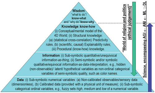
3.4. RTD of big data cube management systems and AGI as two sides of the same coin, that are closely related to each other and cannot be separated

Following the in-depth analysis of the fundamental DIKW conceptualization (see Figure 16) proposed in Subsection 3.3, the notion of big data is worth a detailed discussion.

Typically employed in both scientific and non-scientific domains as a buzzword featuring shallow meaning, big data are either numerical or categorical variables (refer to Subsection 3.3.1) characterized by the six Vs of volume, variety, veracity, velocity, volatility and value (Metternicht et al., 2020). Because no big data can be realistically processed and interpreted by traditional data processing systems and/or human labor, then the notion of big data always implies (requires) AGI = Equation (5)(5) $\text{lsquo}\mathrm{A}\mathrm{R}\mathrm{D}\subset \mathrm{E}\mathrm{O}\text{-}\mathrm{I}\mathrm{U}\subset \mathrm{C}\mathrm{V}\subset \mathrm{A}\mathrm{G}\mathrm{I}\leftarrow \mathrm{A}\mathrm{N}\mathrm{I}\leftarrow \mathrm{M}\mathrm{L}\supset \mathrm{D}\mathrm{L}\supset \mathrm{D}\mathrm{e}\mathrm{e}\mathrm{p}\mathrm{C}\mathrm{o}\mathrm{n}\mathrm{v}\mathrm{o}\mathrm{l}\mathrm{u}\mathrm{t}\mathrm{i}\mathrm{o}\mathrm{n}\mathrm{a}\mathrm{l}\mathrm{N}\mathrm{e}\mathrm{u}\mathrm{r}\mathrm{a}\mathrm{l}\mathrm{N}\mathrm{e}\mathrm{t}\mathrm{w}\mathrm{o}\mathrm{r}\mathrm{k}\left(\mathrm{D}\mathrm{C}\mathrm{N}\mathrm{N}\right)\text{rsquo}$(5) for “good” analysis (interpretation, understanding), characterized by low bias (error rate) and low variance (dependence on input data) jointly (see Figure 13), where AGI should never be confused with ANI = Equation (6)(6) $x0026;\text{ANI=}[\text{DCNN}\subset \text{DL}\subset \text{ML}\text{logical0OR}\text{Traditional}\text{deductive}ArtificialIntelligencex0026;(\text{static}\text{expert}\text{systems},\text{non0adaptive}\text{to}\text{data},\text{also}\text{known}\text{as}\text{Good}\text{Old0Fashioned}x0026;ArtificialIntelligence,\text{GOFAI}]$(6) , acknowledged that “currently deployed Artificial Intelligence systems are examples of ANI” (refer to references listed in Section 2), where ANI is synonym for “narrow idiot savant” (Langley, 2012), capable of low bias, but inherently affected by high variance (low robustness to changes in input data, low scalability to changes in user requirements and/or sensor specifications, low transferability, low extrapolation capability) (refer to Subsection 3.1). Since interpretation of big data always requires AGI = Equation (5)(5) $\text{lsquo}\mathrm{A}\mathrm{R}\mathrm{D}\subset \mathrm{E}\mathrm{O}\text{-}\mathrm{I}\mathrm{U}\subset \mathrm{C}\mathrm{V}\subset \mathrm{A}\mathrm{G}\mathrm{I}\leftarrow \mathrm{A}\mathrm{N}\mathrm{I}\leftarrow \mathrm{M}\mathrm{L}\supset \mathrm{D}\mathrm{L}\supset \mathrm{D}\mathrm{e}\mathrm{e}\mathrm{p}\mathrm{C}\mathrm{o}\mathrm{n}\mathrm{v}\mathrm{o}\mathrm{l}\mathrm{u}\mathrm{t}\mathrm{i}\mathrm{o}\mathrm{n}\mathrm{a}\mathrm{l}\mathrm{N}\mathrm{e}\mathrm{u}\mathrm{r}\mathrm{a}\mathrm{l}\mathrm{N}\mathrm{e}\mathrm{t}\mathrm{w}\mathrm{o}\mathrm{r}\mathrm{k}\left(\mathrm{D}\mathrm{C}\mathrm{N}\mathrm{N}\right)\text{rsquo}$(5) in operational mode (refer to Section 2), capable of low bias jointly with low variance, differently from ANI = Equation (6)(6) $x0026;\text{ANI=}[\text{DCNN}\subset \text{DL}\subset \text{ML}\text{logical0OR}\text{Traditional}\text{deductive}ArtificialIntelligencex0026;(\text{static}\text{expert}\text{systems},\text{non0adaptive}\text{to}\text{data},\text{also}\text{known}\text{as}\text{Good}\text{Old0Fashioned}x0026;ArtificialIntelligence,\text{GOFAI}]$(6) , then big data and AGI can be regarded as two sides of the same coin; the former, big data, always implies the latter, AGI, so that these two concepts cannot be separated.

This inference is neither trivial nor obvious. It is in contrast with a wide audience, ranging from public media to scientists and practitioners, where buzzword big data is almost never one-to-one related to AGI = Equation (5)(5) $\text{lsquo}\mathrm{A}\mathrm{R}\mathrm{D}\subset \mathrm{E}\mathrm{O}\text{-}\mathrm{I}\mathrm{U}\subset \mathrm{C}\mathrm{V}\subset \mathrm{A}\mathrm{G}\mathrm{I}\leftarrow \mathrm{A}\mathrm{N}\mathrm{I}\leftarrow \mathrm{M}\mathrm{L}\supset \mathrm{D}\mathrm{L}\supset \mathrm{D}\mathrm{e}\mathrm{e}\mathrm{p}\mathrm{C}\mathrm{o}\mathrm{n}\mathrm{v}\mathrm{o}\mathrm{l}\mathrm{u}\mathrm{t}\mathrm{i}\mathrm{o}\mathrm{n}\mathrm{a}\mathrm{l}\mathrm{N}\mathrm{e}\mathrm{u}\mathrm{r}\mathrm{a}\mathrm{l}\mathrm{N}\mathrm{e}\mathrm{t}\mathrm{w}\mathrm{o}\mathrm{r}\mathrm{k}\left(\mathrm{D}\mathrm{C}\mathrm{N}\mathrm{N}\right)\text{rsquo}$(5) . At best, big data are positively correlated with “currently deployed Artificial Intelligence systems” (EC – European Commission, 2019), which are instances of ‘ANI ← ML ⊃ DL’ = Equation (6)(6) $x0026;\text{ANI=}[\text{DCNN}\subset \text{DL}\subset \text{ML}\text{logical0OR}\text{Traditional}\text{deductive}ArtificialIntelligencex0026;(\text{static}\text{expert}\text{systems},\text{non0adaptive}\text{to}\text{data},\text{also}\text{known}\text{as}\text{Good}\text{Old0Fashioned}x0026;ArtificialIntelligence,\text{GOFAI}]$(6) (see Figure 17), but ANI is only part-without-inheritance-of AGI, i.e. semantic relationship ‘DL ⊂ ML → ANI → AGI ⊂ Cognitive science’ = Equation (5)(5) $\text{lsquo}\mathrm{A}\mathrm{R}\mathrm{D}\subset \mathrm{E}\mathrm{O}\text{-}\mathrm{I}\mathrm{U}\subset \mathrm{C}\mathrm{V}\subset \mathrm{A}\mathrm{G}\mathrm{I}\leftarrow \mathrm{A}\mathrm{N}\mathrm{I}\leftarrow \mathrm{M}\mathrm{L}\supset \mathrm{D}\mathrm{L}\supset \mathrm{D}\mathrm{e}\mathrm{e}\mathrm{p}\mathrm{C}\mathrm{o}\mathrm{n}\mathrm{v}\mathrm{o}\mathrm{l}\mathrm{u}\mathrm{t}\mathrm{i}\mathrm{o}\mathrm{n}\mathrm{a}\mathrm{l}\mathrm{N}\mathrm{e}\mathrm{u}\mathrm{r}\mathrm{a}\mathrm{l}\mathrm{N}\mathrm{e}\mathrm{t}\mathrm{w}\mathrm{o}\mathrm{r}\mathrm{k}\left(\mathrm{D}\mathrm{C}\mathrm{N}\mathrm{N}\right)\text{rsquo}$(5) holds.

Figure 17. Adapted from (Camara, 2017). Google Trends: Big data vs Machine learning (ML) search trends, May 6, 2012 – May 6, 2017.

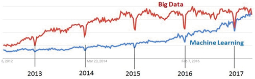
Whereas big data are impossible to be dealt with by traditional data processing systems and/or human labor and require AGI for “good” interpretation (featuring low bias and low variance jointly, see Figure 13), it is important to stress that the vice versa does not hold, i.e. AGI is required to perform “well” (featuring low bias and low variance jointly) upon:

• Big data, characterized by the six Vs of volume, variety, veracity, velocity, volatility and value (Metternicht et al., 2020) and, by now (see Figure 17), higly correlated with “currently deployed Artificial Intelligence systems” (EC – European Commission, 2019), which are instances of ‘ANI ← ML ⊃ DL’ = Equation (6)(6) $x0026;\text{ANI=}[\text{DCNN}\subset \text{DL}\subset \text{ML}\text{logical0OR}\text{Traditional}\text{deductive}ArtificialIntelligencex0026;(\text{static}\text{expert}\text{systems},\text{non0adaptive}\text{to}\text{data},\text{also}\text{known}\text{as}\text{Good}\text{Old0Fashioned}x0026;ArtificialIntelligence,\text{GOFAI}]$(6) ,

as well as

• Small data (see Figure 18), in agreement with:

  • Biological intelligence, which is capable of few-sample (few-shot) learning (Bills, 2020; Gonfalonieri, 2019; Parisi, 1991; Piaget, 1970; Practical AI, 2020). In the words by Melanie Mitchell: “The problem [of DL] is that you have already lost the battle if you are having to train it on thousands and thousands of examples. That is not what abstraction is all about. It is all about what people in machine learning call ‘few-shot learning,’ which means you learn on a very small number of examples. That is what abstraction is really for … where you cannot learn any weird statistical correlations because all you have [are few] examples” (Marks, 2021).

  • The property of systematicity of language/thought, which is related to the property of compositionality, considered at the basis of real understanding of natural language by prominent cognitive scientists, logicians and philosophers of science (Fodor, 1998; Peirce, 1994; Rescorla, 2019; Saba, 2020a). In the terminology of philosophy and linguistics, “it has been proven long time ago that understanding (intended as know how, alternative to know what, refer to Subsection 3.1) is systematic: if I know/understand what some expression/syntactic pattern means, then I must know what infinitely similar expression/syntactic pattern means – and if I ‘know’ one, but not the other, then I have simply memorized one, but not the other and thus there is no real understanding … Here is the corresponding argument in natural language: no one can entertain the thought (or equivalently, truly understand the meaning of) ‘John loves Mary’ without being able to entertain the thought (or equivalently, understand the meaning of) ‘Mary loves John’, ‘John loves John’, ‘Someone loves John’, ‘Mary loves someone’, etc.” (Saba, 2020b).

Figure 18. Lesson to be learned from big data analysis, required to cope with the six Vs of volume, velocity, variety, veracity, volatility and value (Metternicht et al., 2020). For example, the popular Google Earth Engine (Gorelick et al., 2017) is typically considered a valuable instance of the set of algorithms suitable for working on EO large image databases. Noteworthy, the Google Earth Engine typically adopts a pixel-based-through-time image analysis approach, synonym for spatial-context insensitive 1D image analysis. The computer vision (CV) and remote sensing (RS) communities have been striving to abandon 1D analysis of (2D) imagery since the 1970s (Nagao & Matsuyama, 1980). In spite of these efforts, to date, in the RS common practice, traditional suboptimal algorithms for 1D analysis of (2D) imagery implemented in the Google Earth Engine platform are considered the state-of-the-art in EO big data cube analysis (Gorelick et al., 2017). Only a small subset of data processing algorithms scores “(fuzzy) high” in a minimally dependent maximally informative (mDMI) set of outcome and process quantitative quality indicators (OP-Q²Is), including accuracy, efficiency, robustness to changes in input data, robustness to changes in input parameters, scalability, timeliness, costs and value (Baraldi, 2017; Baraldi & Boschetti, 2012a, 2012b; Baraldi et al., 2014, 2018a, 2018b; Baraldi & Tiede, 2018a, 2018b) (refer to Subsection 3.1), in both small data analysis and big data analysis. Only this small subset of data processing algorithms belongs to the domain of interest of Artificial General Intelligence (AGI) = Equation (5)(5) $\text{lsquo}\mathrm{A}\mathrm{R}\mathrm{D}\subset \mathrm{E}\mathrm{O}\text{-}\mathrm{I}\mathrm{U}\subset \mathrm{C}\mathrm{V}\subset \mathrm{A}\mathrm{G}\mathrm{I}\leftarrow \mathrm{A}\mathrm{N}\mathrm{I}\leftarrow \mathrm{M}\mathrm{L}\supset \mathrm{D}\mathrm{L}\supset \mathrm{D}\mathrm{e}\mathrm{e}\mathrm{p}\mathrm{C}\mathrm{o}\mathrm{n}\mathrm{v}\mathrm{o}\mathrm{l}\mathrm{u}\mathrm{t}\mathrm{i}\mathrm{o}\mathrm{n}\mathrm{a}\mathrm{l}\mathrm{N}\mathrm{e}\mathrm{u}\mathrm{r}\mathrm{a}\mathrm{l}\mathrm{N}\mathrm{e}\mathrm{t}\mathrm{w}\mathrm{o}\mathrm{r}\mathrm{k}\left(\mathrm{D}\mathrm{C}\mathrm{N}\mathrm{N}\right)\text{rsquo}$(5) , see Figure 9.

The proposed requirement that AGI, by definition, is expected to perform “well”, which means it features low bias (error rate) and low variance (dependence on input data) jointly (see Fig. 13), when input with big data a well as small data (see Fig. 18), in agreement with biological intelligence and with the property of systematicity of natural language/thought (Fodor, 1998; Peirce, 1994; Rescorla, 2019; Saba, 2020a), requires further investigation.

First, on the one hand, a big labeled/supervised data set can be regarded as big in terms of size/cardinality of the sampled data set, despite the fact it can be small, i.e., narrow/specialized/deep, in terms of labeling value/ meaning/ semantics. For example, supervised big data samples are many, but their labels belong to a small vocabulary/ taxonomy(D, L) of semantic elements (Ball, 2021)/ referents (Ball, 2021)/ classes of real world-objects/ entities (Chen, 1976)/ concepts in a conceptual/mental model of a world-“domain of interest, D, from the perspective of a person who uses a language, L, for the purpose of talking about D” (Sowa, 2000, p. 492) (refer to Section 2).

Second, on the other hand, so-called small labeled/supervised data set, although small in terms of size/cardinality, can be either broad/horizontal or narrow/specialized/deep in terms of labeling value/ meaning/ semantics.

Third, AGI is necessary-but-not-sufficient precondition to big data analysis in operational mode, featuring low bias and low variance jointly, see Figure 13. For example, to accomplish an AGI4DIAS = Equation (1)(1) $\begin{array}{rl}& \text{lsquo}\mathrm{A}\mathrm{G}\mathrm{I}\text{-}\mathrm{e}\mathrm{n}\mathrm{a}\mathrm{b}\mathrm{l}\mathrm{e}\mathrm{d}\mathrm{D}\mathrm{I}\mathrm{A}\mathrm{S}=\mathrm{A}\mathrm{G}\mathrm{I}4\mathrm{D}\mathrm{I}\mathrm{A}\mathrm{S}=\mathrm{S}\mathrm{e}\mathrm{m}\mathrm{a}\mathrm{n}\mathrm{t}\mathrm{i}\mathrm{c}\mathrm{s}\text{-}\mathrm{e}\mathrm{n}\mathrm{a}\mathrm{b}\mathrm{l}\mathrm{e}\mathrm{d}\mathrm{D}\mathrm{I}\mathrm{A}\mathrm{S}2.0\\ & (\mathrm{D}\mathrm{I}\mathrm{A}\mathrm{S}{2}^{\mathrm{n}\mathrm{d}}\mathrm{g}\mathrm{e}\mathrm{n}\mathrm{e}\mathrm{r}\mathrm{a}\mathrm{t}\mathrm{i}\mathrm{o}\mathrm{n})=\mathrm{D}\mathrm{I}\mathrm{A}\mathrm{S}2.0=\mathrm{A}\mathrm{G}\mathrm{I}+\mathrm{D}\mathrm{I}\mathrm{A}\mathrm{S}1.0+\mathrm{S}\mathrm{C}\mathrm{B}\mathrm{I}\mathrm{R}+\mathrm{S}\mathrm{E}\mathrm{I}\mathrm{K}\mathrm{D}\text{rsquo}\end{array}$(1) framework in operational mode (refer to Section 2), the integration of an AGI component system with a big data management component system, such as the GEOSS digital Common Infrastructure (see Figure 1), is necessary.

Fourth, AGI is sufficient-but-not-necessary precondition to small data analysis. For example, ANI = Equation (6)(6) $x0026;\text{ANI=}[\text{DCNN}\subset \text{DL}\subset \text{ML}\text{logical0OR}\text{Traditional}\text{deductive}ArtificialIntelligencex0026;(\text{static}\text{expert}\text{systems},\text{non0adaptive}\text{to}\text{data},\text{also}\text{known}\text{as}\text{Good}\text{Old0Fashioned}x0026;ArtificialIntelligence,\text{GOFAI}]$(6) , which is only part-without-inheritance-of AGI = Equation (5)(5) $\text{lsquo}\mathrm{A}\mathrm{R}\mathrm{D}\subset \mathrm{E}\mathrm{O}\text{-}\mathrm{I}\mathrm{U}\subset \mathrm{C}\mathrm{V}\subset \mathrm{A}\mathrm{G}\mathrm{I}\leftarrow \mathrm{A}\mathrm{N}\mathrm{I}\leftarrow \mathrm{M}\mathrm{L}\supset \mathrm{D}\mathrm{L}\supset \mathrm{D}\mathrm{e}\mathrm{e}\mathrm{p}\mathrm{C}\mathrm{o}\mathrm{n}\mathrm{v}\mathrm{o}\mathrm{l}\mathrm{u}\mathrm{t}\mathrm{i}\mathrm{o}\mathrm{n}\mathrm{a}\mathrm{l}\mathrm{N}\mathrm{e}\mathrm{u}\mathrm{r}\mathrm{a}\mathrm{l}\mathrm{N}\mathrm{e}\mathrm{t}\mathrm{w}\mathrm{o}\mathrm{r}\mathrm{k}\left(\mathrm{D}\mathrm{C}\mathrm{N}\mathrm{N}\right)\text{rsquo}$(5) , can be adopted for small data analysis, where low bias is pursued, but high variance (low robustness to changes in input data, low scalability to changes in user requirements and/or sensor specifications, low transferability, low extrapolation capability) is tolerated.

These working hypotheses about big data and AGI, stemming from the original semantic relationship ‘Cognitive science ⊃ AGI ← ANI ← ML ⊃ DL’ = Equation (5)(5) $\text{lsquo}\mathrm{A}\mathrm{R}\mathrm{D}\subset \mathrm{E}\mathrm{O}\text{-}\mathrm{I}\mathrm{U}\subset \mathrm{C}\mathrm{V}\subset \mathrm{A}\mathrm{G}\mathrm{I}\leftarrow \mathrm{A}\mathrm{N}\mathrm{I}\leftarrow \mathrm{M}\mathrm{L}\supset \mathrm{D}\mathrm{L}\supset \mathrm{D}\mathrm{e}\mathrm{e}\mathrm{p}\mathrm{C}\mathrm{o}\mathrm{n}\mathrm{v}\mathrm{o}\mathrm{l}\mathrm{u}\mathrm{t}\mathrm{i}\mathrm{o}\mathrm{n}\mathrm{a}\mathrm{l}\mathrm{N}\mathrm{e}\mathrm{u}\mathrm{r}\mathrm{a}\mathrm{l}\mathrm{N}\mathrm{e}\mathrm{t}\mathrm{w}\mathrm{o}\mathrm{r}\mathrm{k}\left(\mathrm{D}\mathrm{C}\mathrm{N}\mathrm{N}\right)\text{rsquo}$(5) proposed as postulate (axiom, first-principle) in Section 2, agree with Melanie Mitchell’s quote (reported in Section 2): “Unlocking Artificial Intelligence’s barrier of meaning [semantics] is likely to require a step backward for the field, away from ever bigger networks and data collections, and back to the field’s roots as an interdisciplinary [cognitive] science studying the most challenging of scientific problems: the nature of intelligence” (Mitchell, 2019).

The observation (true-fact) that big data require an AGI as necessary-but-not-sufficient precondition for accomplishing big data interpretation is tantamount to saying that the collection of big data “does not make (full) logical sense” if there is no AGI available in advance, capable of fulfilling an inherently ill-posed/ qualitative/ equivocal/ difficult information-as-data-interpretation task (Capurro & Hjørland, 2003) (refer to Subsection 3.3.3).

This observation is oversighted by the human community as a whole, including the scientific community, where big data acquisition, storage and transmission come first while AGI, necessary for big data interpretation, comes later. Actually, AGI comes never. In fact, AGI has not been accomplished yet, because “currently deployed Artificial Intelligence systems are examples of ANI” (refer to references listed in Section 2), where ANI is synonym for “narrow idiot savant” (Langley, 2012), capable of low bias, but inherently affected by high variance (refer to Subection 3.1), see Figure 11. Until now, the major portion of the intellectual, financial and technological efforts carried out by both private and public sectors has been focusing on the RTD of yet-another quantitative information-as-thing infrastructure (refer to Subsection 3.3.3), capable of big sensory data acquisition, storage and transmission, such as the EC DIAS 1.0 at the European continental scale (EU – European Union, 2017, 2018), the fifth-generation (5G) wireless technology for digital cellular networks, etc., rather than on developing the first AGI infrastructure, pertaining to the inherently ill-posed/ qualitative/ equivocal domain of information-as-data-interpretation (refer to Subsection 3.3.3) and consisting of a hardware/electronic brain component system in combination with a software/artificial mind component system, in agreement with the “connectionists approach”, synonym for “artificial mind in electronic brain” paradigm, promoted by traditional cybernetics (Baraldi, 2017; Jordan, 2018; Langley, 2012; Serra & Zanarini, 1990; Westphal, 2016) (refer to Section 2).

The logical explanation of this ongoing situation is that Shannon’s data acquisition and communication problems (Shannon, 1948) in the quantitative/unequivocal domain of information-as-thing are better conditioned than, and therefore are (so-to-speak) much easier to solve than, inherently ill-posed AGI problems in the qualitative/equivocal domain of information-as-data-interpretation (refer to Subsection 3.3.3). The consequence of this ongoing situation is twofold.

On the one hand, since the 1950s, first, the data transmission/communication technology has reached its fifth-generation 5G infrastructure. Second, the quality and quantity of spaceborne, airborne and terrestrial EO big data acquired by the RS community have been ever increasing (Belward & Skøien, 2015; Manilici, Kiemle, Reck, & Winkler, 2013; NASA – National Aeronautics and Space Administration, 2016; Pinna & Ferrante, 2009), apparently according to the Moore exponential law of productivity (Ball, 2013), see Figure 19(a).

Figure 19. (a) Adapted from (Manilici et al., 2013). Deutsches Zentrum für Luft- und Raumfahrt (German Aerospace Center, DLR) archive size in petabytes (PB) of optical and synthetic aperture radar (SAR) data acquired by spaceborne imaging sensors. Status on July 30, 2013. Also refer to (Belward & Skøien, 2015; NASA – National Aeronautics and Space Administration, 2016; Pinna & Ferrante, 2009). (b) Global European annual satellite EO products and services turnover, in millions of euros (eoVox, 2008). Unfortunately, this latter estimate, which is monotonically increasing with the number of EO data users, provides no clue at all on the average per user productivity, monotonically increasing with the average number of different EO images actually used (interpreted, rather than downloaded) by a single user per year. Our conjecture is that existing suboptimal EO image understanding (EO-IU) systems, not provided with the Artificial General Intelligence (AGI) capability required to accomplish EO big data interpretation in operational mode (see Figure 18), have been outpaced in productivity by the exponential rate of collection of EO sensory data, whose quality and quantity are ever-increasing, see Figure 19(a).

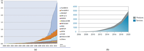
On the other hand, has this exponential increase in EO big data availability, accessibility and suitability come together with an exponential increase in AGI capability, if any? Unfortunately, no … (e.g. refer to Appendix I to Appendix V on an increasing disillusionment about ‘DL ⊂ ML → ANI → AGI’ solutions).

Our conjecture is that, supported by no AGI, humans are overwhelmed by big sensory subsymbolic data they are unable to interpret (transform into useful information-as-data-interpretation). Due to lack of AGI, humans blame the big data and ask for even bigger data, whose quantity and quality increase exponentially … which makes the semantic gap (Matsuyama & Hwang, 1990) to fill from sensory data to information-as-data-interpretation monotonically increasing through time.

When applied to the RS meta-science domain (refer to Section 2), the conjecture above means that the capability of the RS community to accomplish the qualitative/ equivocal/ inherently ill-posed (difficult) cognitive task of information-as-data-interpretation has always been outpaced by the rate of collection of EO big sensory data, whose six Vs are ever increasing (Metternicht et al., 2020), see Figure 19(a).

To prove this conjecture, let us consider that, back in 2002, the percentage of EO big data ever downloaded from the ESA databases was estimated at about 10% or less (ESA - European Space Agency, D’Elia, S., Personal communication, 2002). Data downloading does not imply data use, meaning data interpretation. This observation is tantamount to saying that when EO data users were mainly institutional stakeholders, which means “few” in number (for reason of simplicity, let us think of one single end-user of the ESA data, back in year 2002), more than 90% of the EO sensory data ever collected by ESA was totally ignored (never accessed to for interpretation purposes) until year 2002. From year 2002 to 2020, first, the number of EO data users, either institutional or private, has been monotonically increasing; second, the rate of collection of EO data has been exponentially increasing, see Figure 19(a); third, unfortunately, no AGI has been achieved yet, to support humans in big data interpretation. Hence, an average EO data exploitation factor, equal to the amount of available big data divided by the ability to interpret data per single user, updated to year 2020 is realistically estimated to be lower than the (optimistic) 10% value scored back in 2002 (by an idealistic single user). This estimate implies that, in the RS common practice, past and present suboptimal EO-IU systems, not pertaining to the AGI = Equation (5)(5) $\text{lsquo}\mathrm{A}\mathrm{R}\mathrm{D}\subset \mathrm{E}\mathrm{O}\text{-}\mathrm{I}\mathrm{U}\subset \mathrm{C}\mathrm{V}\subset \mathrm{A}\mathrm{G}\mathrm{I}\leftarrow \mathrm{A}\mathrm{N}\mathrm{I}\leftarrow \mathrm{M}\mathrm{L}\supset \mathrm{D}\mathrm{L}\supset \mathrm{D}\mathrm{e}\mathrm{e}\mathrm{p}\mathrm{C}\mathrm{o}\mathrm{n}\mathrm{v}\mathrm{o}\mathrm{l}\mathrm{u}\mathrm{t}\mathrm{i}\mathrm{o}\mathrm{n}\mathrm{a}\mathrm{l}\mathrm{N}\mathrm{e}\mathrm{u}\mathrm{r}\mathrm{a}\mathrm{l}\mathrm{N}\mathrm{e}\mathrm{t}\mathrm{w}\mathrm{o}\mathrm{r}\mathrm{k}\left(\mathrm{D}\mathrm{C}\mathrm{N}\mathrm{N}\right)\text{rsquo}$(5) domain, but belonging to the ANI = Equation (6)(6) $x0026;\text{ANI=}[\text{DCNN}\subset \text{DL}\subset \text{ML}\text{logical0OR}\text{Traditional}\text{deductive}ArtificialIntelligencex0026;(\text{static}\text{expert}\text{systems},\text{non0adaptive}\text{to}\text{data},\text{also}\text{known}\text{as}\text{Good}\text{Old0Fashioned}x0026;ArtificialIntelligence,\text{GOFAI}]$(6) domain, have been outpaced, in terms of productivity (related to the several OP-Q²Is proposed in Subsection 3.1, including degree of automation, accuracy, efficiency, timeliness and costs), by the exponential rate of collection of EO sensory data, whose quality and quantity are exponentially increasing, see Figure 18(a) (Belward & Skøien, 2015; Manilici et al., 2013; NASA – National Aeronautics and Space Administration, 2016; Pinna & Ferrante, 2009).

A shallow assessment of our conjecture that, in year 2020, an average EO data exploitation (productivity) factor per single user is lower than the (optimistic) 10% value scored back in 2002 may conclude that our estimate is affected by a pessimistic attitude. On the contrary, our conjecture is perfectly compatible with both the annual satellite EO products and services economic turnover, shown in Figure 19(b), and the Copernicus hubs’ Archive Exploitation Ratio monitored by ESA (Serco, 2019). The Archive Exploitation Ratio is defined by ESA as the total number of products which have been published on the whole set of Copernicus hubs (Open Hub, ColHub, IntHub and ServHub) since their start, divided by the total number of users’ downloads made from all these hubs. An Archive Exploitation Ratio estimate is monotonically decreasing with the overall users’ interest, considered equal to the total number of EO data downloads, which is, in turn, monotonically non-decreasing with the number of users. For example, an Archive Exploitation Ratio per Sentinel-2 mission at the end of year 2018 was 1:12 (Serco, 2019). Unfortunately, an Archive Exploitation Ratio estimate provides no clue at all on the average per user productivity, which is the average number of different EO images actually used (interpreted, rather than downloaded) by a single user per year, for either low-level EO image pre-processing (enhancement) tasks and/or high-level EO image interpretation tasks, either semantic (thematic) interpretation or biophysical variable estimation, encompassing ECVs estimation (Bojinski et al., 2014) (see Table 2), which is targeted by the ongoing ESA Climate Change Initiative’s parallel projects (ESA – European Space Agency, 2017b, 2020a, 2020b) (refer to Section 2).

If no ‘AGI ⊃ CV ⊃ EO-IU’ has yet been accomplished to interpret multi-source EO big image databases in operational mode (refer to Section 2), we can conclude that the hundreds of suboptimal EO-IU algorithms presented to date in the scientific literature and/or implemented in either commercial or free-of-cost ‘CV ⊃ EO-IU’ software toolboxes and/or software libraries, acknowledged that the former typically consist of overly complicated collections (libraries) of inductive ML-from-data algorithms to choose from based on heuristics (trial-and-error) (OpenCV, 2020; L3Harris Geospatial, 2009) (refer to Subsection 3.3.2), do not belong to the domain of AGI = Equation (5)(5) $\text{lsquo}\mathrm{A}\mathrm{R}\mathrm{D}\subset \mathrm{E}\mathrm{O}\text{-}\mathrm{I}\mathrm{U}\subset \mathrm{C}\mathrm{V}\subset \mathrm{A}\mathrm{G}\mathrm{I}\leftarrow \mathrm{A}\mathrm{N}\mathrm{I}\leftarrow \mathrm{M}\mathrm{L}\supset \mathrm{D}\mathrm{L}\supset \mathrm{D}\mathrm{e}\mathrm{e}\mathrm{p}\mathrm{C}\mathrm{o}\mathrm{n}\mathrm{v}\mathrm{o}\mathrm{l}\mathrm{u}\mathrm{t}\mathrm{i}\mathrm{o}\mathrm{n}\mathrm{a}\mathrm{l}\mathrm{N}\mathrm{e}\mathrm{u}\mathrm{r}\mathrm{a}\mathrm{l}\mathrm{N}\mathrm{e}\mathrm{t}\mathrm{w}\mathrm{o}\mathrm{r}\mathrm{k}\left(\mathrm{D}\mathrm{C}\mathrm{N}\mathrm{N}\right)\text{rsquo}$(5) because unsuitable for coping with the six Vs of big data analysis.

Belonging to the domain of ANI = Equation (6)(6) $x0026;\text{ANI=}[\text{DCNN}\subset \text{DL}\subset \text{ML}\text{logical0OR}\text{Traditional}\text{deductive}ArtificialIntelligencex0026;(\text{static}\text{expert}\text{systems},\text{non0adaptive}\text{to}\text{data},\text{also}\text{known}\text{as}\text{Good}\text{Old0Fashioned}x0026;ArtificialIntelligence,\text{GOFAI}]$(6) , these hundreds of suboptimal EO-IU algorithms, including increasingly popular ‘DCNN ⊂ DL ⊂ ML → ANI → AGI’ algorithms (see Figure 17), featuring low bias (low error rate), but affected by high variance (high dependence on input data, low transferability, see Figure 13), are eligible for use in EO narrow/ deep/ “vertical”/ specialized/ “easy” data analysis exclusively, equivalent to toy problems (narrow/ deep/ “vertical”/ specialized/ “easy” problems, so to speak), although narrow/ deep/ “vertical”/ specialized data (e.g., spaceborne Sentinel-2 optical imagery, which is different from spaceborne Sentinel-1 Synthetic Aperture Radar imagery, but also from spaceborne Sentinel-3 optical imagery) typically consist of big data (in size, cardinality), see Figure 18.

As explained above, this conclusion is not in contrast with current estimates of the ESA Archive Exploitation Ratio (Serco, 2019) or with the annual satellite EO products and services economic turnover, see Figure 19(b) (eoVox, 2008). Our conjecture is statistically independent of the two aforementioned statistics because not affected by the total number of EO data users, which is ever increasing.

Unfortunately, our inference above has never been acknowledged by the CV and RS meta-science communities, whose RTD efforts remain focused on the domain of ANI = Equation (6)(6) $x0026;\text{ANI=}[\text{DCNN}\subset \text{DL}\subset \text{ML}\text{logical0OR}\text{Traditional}\text{deductive}ArtificialIntelligencex0026;(\text{static}\text{expert}\text{systems},\text{non0adaptive}\text{to}\text{data},\text{also}\text{known}\text{as}\text{Good}\text{Old0Fashioned}x0026;ArtificialIntelligence,\text{GOFAI}]$(6) .

Our conclusion urges the CV and RS meta-science communities to start considering the RTD of ‘Cognitive science ⊃ AGI ⊃ CV ⊃ EO-IU ⊃ ARD’ = Equation (3)(3) $\text{lsquo}\mathrm{A}\mathrm{R}\mathrm{D}\subset \mathrm{E}\mathrm{O}-\mathrm{I}\mathrm{U}\subset \mathrm{C}\mathrm{V}\subset \mathrm{A}\mathrm{G}\mathrm{I}\subset \mathrm{C}\mathrm{o}\mathrm{g}\mathrm{n}\mathrm{i}\mathrm{t}\mathrm{i}\mathrm{v}\mathrm{e}\mathrm{s}\mathrm{c}\mathrm{i}\mathrm{e}\mathrm{n}\mathrm{c}\mathrm{e}\text{rsquo}$(3) solutions in operational mode (refer to Section 2) as their most challenging open problem in the inherently ill-posed and difficult domain of qualitative/equivocal information-as-data-interpretation, to be tackled with highest priority by means of an innovative multi-disciplinary approach to cognitive science (refer to refences listed in Section 2) (see Figure 11), acknowledged that AGI “is not a problem in statistics” (Etzioni, 2017) (refer to Appendix I).

3.5. Bayesian inference constraints for better conditioning an inherently ill-posed AGI system solution, acknowledged that semantic relationhsip ‘Cognitive science ⊃ AGI ⊃ CV ⊃ EO-IU ⊃ ARD’ holds

In line with the GEO visionary goal of an implementation plan for years 2005–2015 of a GEOSS (EC – European Commission and GEO – Group on Earth Observations, 2014; GEO – Group on Earth Observations, 2005, 2019; Mavridis, 2011), unaccomplished to date, revised by a GEO’s second implementation plan for years 2016–2025 of a new GEOSS, regarded as expert EO data-derived information and knowledge system (GEO – Group on Earth Observations, 2015; Nativi et al., 2015, 2020; Santoro et al., 2017) (see Figure 1), this Subsection focuses on the open problem of transforming EO big data, characterized by the six Vs of volume, variety, veracity, velocity, volatility and value (Metternicht et al., 2020), including multi-sensor EO big 2D gridded data (imagery) as special case, into operational, timely and comprehensive VAPS, in agreement with the intergovernmental GEO-CEOS QA4EO Cal/Val requirements (refer to references listed in Section 2) and with the FAIR principles for scholarly/scientific digital data and non-data research objects, see Table 1.

According to the previous Subsections of the present Section 3, transformation of EO big sensory data into operational, timely and comprehensive VAPS is regarded as a qualitative/equivocal cognitive problem of information-as-data-interpretation (Capurro & Hjørland, 2003), inherently ill-posed in the Hadamard sense (Hadamard, 1902), to be coped with by AGI systems (refer to Subsection 3.4), which require a priori knowledge in addition to sensory data to become better posed (better conditioned, better constrained) for numerical solution (Baraldi, 2017; Baraldi et al., 2018a, 2018b; Baraldi & Tiede, 2018a, 2018b; Bishop, 1995; Cherkassky & Mulier, 1998; Dubey et al., 2018), see Figure 11.

In compliance with a Bayesian/ driven-by-prior-knowledge/ class-conditional approach to data analysis (Bowers & Davis, 2012; Ghahramani, 2011; Lähteenlahti, 2021; Quinlan, 2012; Sarkar, 2018) adopted by the Marr constraints proposed in the CV literature (Marr, 1982; Quinlan, 2012), a set of Bayesian constraints is proposed hereafter to better condition an inherently ill-posed AGI system solution, investigated at the Marr five levels of system understanding (refer to Subsection 3.2).

Since semantic relationship ‘AGI ⊃ CV ⊃ EO-IU ⊃ ARD’ = Equation (3)(3) $\text{lsquo}\mathrm{A}\mathrm{R}\mathrm{D}\subset \mathrm{E}\mathrm{O}-\mathrm{I}\mathrm{U}\subset \mathrm{C}\mathrm{V}\subset \mathrm{A}\mathrm{G}\mathrm{I}\subset \mathrm{C}\mathrm{o}\mathrm{g}\mathrm{n}\mathrm{i}\mathrm{t}\mathrm{i}\mathrm{v}\mathrm{e}\mathrm{s}\mathrm{c}\mathrm{i}\mathrm{e}\mathrm{n}\mathrm{c}\mathrm{e}\text{rsquo}$(3) holds, then Bayesian constraints suitable for better conditioning a general-purpose inherently ill-posed AGI system will be inherited by specialized AGI subsystems, such as ‘ARD ⊂ EO-IU ⊂ CV’ systems involved with the inherently ill-posed cognitive (sub)task of vision, synonym for inherently ill-posed scene-from-image reconstruction and understanding, regarded as a specialized information-as-data-interpretation (sub)task (refer to the farther Section 4). In other words, Bayesian constraints inherited from AGI will be eligible for further specialization in the cognitive subdomain of ‘ARD ⊂ EO-IU ⊂ CV’ (sub)tasks (refer to the farther Subsection 4.2).

1. In agreement with an intuitive general-purpose GIGO principle (Baraldi, 2017; Geiger et al., 2021; Thompson, 2018) (refer to Section 2), easy to understand based on commonsense knowledge (refer to references listed in Section 2), with the popular FAIR criteria for scientific data (product and process) management (GO FAIR – International Support and Coordination Office, 2021; Wilkinson et al., 2016) (see Table 1) and with the GEO-CEOS QA4EO Cal requirements (refer to references listed in Section 2), whenever possible, which means whenever sensory data are provided with metadata Cal parameters, sensory data, either big data or small data to be coped with by AGI system solutions in operational mode (see Figure 18), must be calibrated (e.g. radiometrically calibrated) to become better behaved (better conditioned) and better understood, because provided with a physical meaning, a physical unit of measure (e.g. a radiometric unit of measure) and a physical range of change (Baraldi, 2009; Dwyer et al., 2018; Pacifici et al., 2014) (refer to Subsection 3.3.2).

   As reported in Subsection 3.3.2, unlike uncalibrated data, eligible for use in statistical analytics exclusively, such as inductive statistical model-based ‘ML ⊃ DL ⊃ DCNN’ algorithms, calibrated data can be employed as input to deductive/physical model-based inference systems as well as inductive/statistical model-based inference systems as well as hybrid (combined deductive and inductive) inference systems, such as hybrid ‘AGI ⊃ CV ⊃ EO-IU ⊃ ARD’ = Equation (3)(3) $\text{lsquo}\mathrm{A}\mathrm{R}\mathrm{D}\subset \mathrm{E}\mathrm{O}-\mathrm{I}\mathrm{U}\subset \mathrm{C}\mathrm{V}\subset \mathrm{A}\mathrm{G}\mathrm{I}\subset \mathrm{C}\mathrm{o}\mathrm{g}\mathrm{n}\mathrm{i}\mathrm{t}\mathrm{i}\mathrm{v}\mathrm{e}\mathrm{s}\mathrm{c}\mathrm{i}\mathrm{e}\mathrm{n}\mathrm{c}\mathrm{e}\text{rsquo}$(3) system solutions in the multi-disciplinary domain of cognitive science, see Figure 11(a).

   As reported in Subsection 3.3.2, in the RS meta-science domain, a second technical advantage of the radiometric Cal of EO optical big 2D gridded data (imagery) is that, whereas optical sensory data at EO Level 0 are dimensionless DNs ≥ 0 typically encoded as unsigned short int, DNs radiometrically calibrated into ‘TOARF ∈ [0.0, 1.0] at EO Level 1 ⊇ SURF ∈ [0.0, 1.0] at EO Level 2/(current) ARD ⊇ surface albedo ∈ [0.0, 1.0] at, say, EO Level 3/next generation ARD’ = Equation (8)(8) $\begin{array}{rl}& \text{lsquo}\mathrm{D}\mathrm{N}\mathrm{s}\ge 0\mathrm{a}\mathrm{t}\mathrm{E}\mathrm{O}\mathrm{L}\mathrm{e}\mathrm{v}\mathrm{e}\mathrm{l}0\supseteq \mathrm{T}\mathrm{O}\mathrm{A}\mathrm{R}\mathrm{F}\in \left[0.0,1.0\right]\mathrm{a}\mathrm{t}\mathrm{E}\mathrm{O}\mathrm{L}\mathrm{e}\mathrm{v}\mathrm{e}\mathrm{l}1\supseteq \mathrm{S}\mathrm{U}\mathrm{R}\mathrm{F}\in \left[0.0,1.0\right]\\ & \mathrm{a}\mathrm{t}\mathrm{E}\mathrm{O}\mathrm{L}\mathrm{e}\mathrm{v}\mathrm{e}\mathrm{l}2/\left(\mathrm{c}\mathrm{u}\mathrm{r}\mathrm{r}\mathrm{e}\mathrm{n}\mathrm{t}\right)\mathrm{A}\mathrm{R}\mathrm{D}\supseteq \mathrm{S}\mathrm{u}\mathrm{r}\mathrm{f}\mathrm{a}\mathrm{c}\mathrm{e}\mathrm{a}\mathrm{l}\mathrm{b}\mathrm{e}\mathrm{d}\mathrm{o}\in \left[0.0,1.0\right]\mathrm{a}\mathrm{t},\mathrm{s}\mathrm{a}\mathrm{y},\mathrm{E}\mathrm{O}\mathrm{L}\mathrm{e}\mathrm{v}\mathrm{e}\mathrm{l}3/\mathrm{n}\mathrm{e}\mathrm{x}\mathrm{t}\\ & \mathrm{g}\mathrm{e}\mathrm{n}\mathrm{e}\mathrm{r}\mathrm{a}\mathrm{t}\mathrm{i}\mathrm{o}\mathrm{n}\mathrm{A}\mathrm{R}\mathrm{D}\text{rsquo}& (8)\end{array}$(8) can be encoded as unsigned byte into the discrete and finite range of change {0, 255}, with a negligible data quantization error ≈ 0.2% while reducing memory occupation by 50% (Baraldi, 2017; Baraldi & Tiede, 2018a).

   A third technical consideration implied by Equation (8)(8) $\begin{array}{rl}& \text{lsquo}\mathrm{D}\mathrm{N}\mathrm{s}\ge 0\mathrm{a}\mathrm{t}\mathrm{E}\mathrm{O}\mathrm{L}\mathrm{e}\mathrm{v}\mathrm{e}\mathrm{l}0\supseteq \mathrm{T}\mathrm{O}\mathrm{A}\mathrm{R}\mathrm{F}\in \left[0.0,1.0\right]\mathrm{a}\mathrm{t}\mathrm{E}\mathrm{O}\mathrm{L}\mathrm{e}\mathrm{v}\mathrm{e}\mathrm{l}1\supseteq \mathrm{S}\mathrm{U}\mathrm{R}\mathrm{F}\in \left[0.0,1.0\right]\\ & \mathrm{a}\mathrm{t}\mathrm{E}\mathrm{O}\mathrm{L}\mathrm{e}\mathrm{v}\mathrm{e}\mathrm{l}2/\left(\mathrm{c}\mathrm{u}\mathrm{r}\mathrm{r}\mathrm{e}\mathrm{n}\mathrm{t}\right)\mathrm{A}\mathrm{R}\mathrm{D}\supseteq \mathrm{S}\mathrm{u}\mathrm{r}\mathrm{f}\mathrm{a}\mathrm{c}\mathrm{e}\mathrm{a}\mathrm{l}\mathrm{b}\mathrm{e}\mathrm{d}\mathrm{o}\in \left[0.0,1.0\right]\mathrm{a}\mathrm{t},\mathrm{s}\mathrm{a}\mathrm{y},\mathrm{E}\mathrm{O}\mathrm{L}\mathrm{e}\mathrm{v}\mathrm{e}\mathrm{l}3/\mathrm{n}\mathrm{e}\mathrm{x}\mathrm{t}\\ & \mathrm{g}\mathrm{e}\mathrm{n}\mathrm{e}\mathrm{r}\mathrm{a}\mathrm{t}\mathrm{i}\mathrm{o}\mathrm{n}\mathrm{A}\mathrm{R}\mathrm{D}\text{rsquo}& (8)\end{array}$(8) is that if an ‘AGI ⊃ CV ⊃ EO-IU ⊃ ARD‘ system is capable of coping with input EO imagery radiometrically calibrated into “noisy” TOARF values, then it is also able (i.e., it can be reused, which augments reusability) to interpret (map) input EO imagery radiometrically calibrated into “less noisy” SURF 1-of-3 values where, for example, “radiometric noise” due to atmospheric conditions is either zero, due to clear-sky conditions, or reduced to zero by an EO data pre-processing (enhancement) stage capable of atmospheric effects removal (refer to Subsection 3.3.2).

   In spite of the aforementioned commonsense knowledge about the unequivocal technical advantages of calibrated sensory data over uncalibrated sensory data (refer to Subsection 3.3.2), a Cal data requirement for ‘AGI ⊃ CV ⊃ EO-IU ⊃ ARD’ = Equation (3)(3) $\text{lsquo}\mathrm{A}\mathrm{R}\mathrm{D}\subset \mathrm{E}\mathrm{O}-\mathrm{I}\mathrm{U}\subset \mathrm{C}\mathrm{V}\subset \mathrm{A}\mathrm{G}\mathrm{I}\subset \mathrm{C}\mathrm{o}\mathrm{g}\mathrm{n}\mathrm{i}\mathrm{t}\mathrm{i}\mathrm{v}\mathrm{e}\mathrm{s}\mathrm{c}\mathrm{i}\mathrm{e}\mathrm{n}\mathrm{c}\mathrm{e}\text{rsquo}$(3) system solutions is neither obvious nor trivial. For example, it goes against large portions of the literature and the common practice in meta-sciences like ML and RS, where inductive statistical model-based ‘ML ⊃ DL ⊃ DCNN’ algorithms are increasingly adopted as ‘CV ⊃ EO-IU ⊃ ARD’ system solutions.

   On the one hand, in the RS literature, large portions of published papers coping with EO-IU tasks never mention the notion of “(radiometric) calibration”. For example, in a survey of EO image classification systems published in the RS literature in year 2014 (Ghosh & Kaabouch, 2014), word “calibration” is absent and radiometric Cal tasks are totally ignored (refer to Subsection 3.3.2). On the other hand, in the RS common practice, commercial or free-of-cost EO data processing software toolboxes typically consist of overly complicated collections (libraries) of inductive/statistical model-based ML-from-data algorithms to choose from based on heuristics (trial-and-error) (OpenCV, 2020; L3Harris Geospatial, 2009), which require as input no data radiometrically calibrated to be provided with a radiometric unit of physical measure (Baraldi, 2009, 2017; Baraldi & Boschetti, 2012a, 2012b; Baraldi et al., 2014; Pacifici et al., 2014) (refer to Subsection 3.3.2).

   Our enigmatic conclusion is that EO data radiometric Cal issues are either ignored or oversighted by large portions of the RS literature and in the RS common practice, although radiometric Cal is considered a well-known “prerequisite for physical model-based analysis of airborne and satellite sensor measurements in the optical domain” (Schaepman-Strub et al., 2006), in compliance with the intergovernmental GEO-CEOS QA4EO Cal requirements and with the popular FAIR guiding principles for scientific data (product and process) management, see Table 1. The lack of radiometric Cal requirements specification and implementation typically occurs when the RS meta-science community adopts inductive statistical model-based ‘ML ⊃ DL ⊃ DCNN’ solutions, because statistical model-based algorithms do not require as input data provided with a physical meaning, although robustness to changes in input data of statistical analytics can benefit from data better behaved (better conditioned), because calibrated (refer to Subsection 3.3.2).

2. In compliance with the FAIR criteria for scientific data (product and process) management (see Table 1), AGI solutions are required to adopt the engineering principles of structured system design, specifically, modularity, hierarchy and regularity, recommended for system scalability (Lipson, 2007; Page-Jones, 1988) (refer to Section 2). Structured system design, including structured network-of-networks architectures combining intra-network cooperation with inter-network competition mechanisms to pursue per-network specialization (Baraldi, 2017; Baraldi & Alpaydin, 2002a, 2002b; Fritzke, 1997; Martinetz et al., 1994), guarantees “high” interpretability/ traceability/ accountability/ explainability of the model/solution (Koehrsen, 2018; Lukianoff, 2019) (refer to Subsection 3.1), in contrast with “the black box problem” typically affecting inductive end-to-end learning-from-data ANNs (Baraldi & Tiede, 2018a, 2018b; Lukianoff, 2019; Marcus, 2018, 2020), encompassing increasingly popular ‘DCNN ⊂ DL ⊂ ML’ solutions (Cimpoi et al., 2014; Krizhevsky et al., 2012), see Figure 14.

3. By reverse engineering “the inner workings of the human brain – the only existing proof that such an intelligence is even possible” (Hassabis et al., 2017), acknowledged that in biological cognitive systems “there is never an absolute beginning” (Piaget, 1970), AGI relies upon a hybrid inference paradigm (refer to references listed in Subsection 3.3.2), where deductive/ top-down/ physical model-driven and inductive/ bottom-up/ statistical data-driven inference subsystems are combined, such that top-down/a priori knowledge (like genotype) provides initial conditions to inductive learning-from-examples capabilities (like phenotype), to take advantage of each and overcome their shortcomings (refer to Subsection 3.3.2). According to semantic relationship ‘DCNN ⊂ DL ⊂ ML → ANI → AGI ⊂ Cognitive science’ = Equation (5)(5) $\text{lsquo}\mathrm{A}\mathrm{R}\mathrm{D}\subset \mathrm{E}\mathrm{O}\text{-}\mathrm{I}\mathrm{U}\subset \mathrm{C}\mathrm{V}\subset \mathrm{A}\mathrm{G}\mathrm{I}\leftarrow \mathrm{A}\mathrm{N}\mathrm{I}\leftarrow \mathrm{M}\mathrm{L}\supset \mathrm{D}\mathrm{L}\supset \mathrm{D}\mathrm{e}\mathrm{e}\mathrm{p}\mathrm{C}\mathrm{o}\mathrm{n}\mathrm{v}\mathrm{o}\mathrm{l}\mathrm{u}\mathrm{t}\mathrm{i}\mathrm{o}\mathrm{n}\mathrm{a}\mathrm{l}\mathrm{N}\mathrm{e}\mathrm{u}\mathrm{r}\mathrm{a}\mathrm{l}\mathrm{N}\mathrm{e}\mathrm{t}\mathrm{w}\mathrm{o}\mathrm{r}\mathrm{k}\left(\mathrm{D}\mathrm{C}\mathrm{N}\mathrm{N}\right)\text{rsquo}$(5) adopted herein as working hypothesis, hybrid (combined deductive/physical model-based and inductive/statistical model-based) inference is alternative to inductive end-to-end ‘ML ⊃ DL ⊃ DCNN’ algorithms (Bishop, 1995; Cherkassky & Mulier, 1998; Claire, 2019; Copeland, 2016; Krizhevsky et al., 2012; Sonka et al., 1994).

4. An AGI inference engine exploits four inference mechanisms: deduction, abduction, induction and transitivity (Laurini & Thompson, 1992; Peirce, 1994) (refer to Subsection 3.3.4). This is in contrast with the recent hype on inductive end-to-end ‘DCNN ⊂ DL ⊂ ML’ solutions (Cimpoi et al., 2014; Krizhevsky et al., 2012).

5. In agreement with the intergovernmental GEO-CEOS QA4EO Val requirements (GEO-CEOS – Group on Earth Observations and Committee on Earth Observation Satellites, 2010), AGI solutions pursue inherently ill-posed multi-objective optimization of a community-agreed mDMI set of OP-Q²Is (Baraldi, 2017; Baraldi et al., 2018a, 2018b; Baraldi & Tiede, 2018a, 2018b) (refer to Subsection 3.1), where bias (error rate) and variance (dependence on input data) are required to be jointly minimized (Bishop, 1995; Cherkassky & Mulier, 1998; Geman et al., 1992; Mahadevan, 2019; Sarkar, 2018; Wolpert, 1996; Wolpert & Macready, 1997) (see Figure 13), when input with big data as well as small data sets, see Figure 18 (refer to Subsection 3.4). This is in contrast with the recent hype on ‘DCNN ⊂ DL ⊂ ML’ algorithms (Cimpoi et al., 2014; Krizhevsky et al., 2012), typically characterized by low bias, but high variance and where “big data is never big enough” (Yuille & Liu, 2019) (refer to Subsection 3.1).

4. Background knowledge of the RS meta-science in coping with ‘EO-IU ⊂ CV ⊂ AGI’ cognitive tasks

At the first level of an “augmented” DIKW pyramid (see Figure 16), the notion of big data, characterized by the six Vs of volume, variety, veracity, velocity, volatility and value (Metternicht et al., 2020), includes as special case the notion of big 2D gridded data (imagery) (Baraldi, 2017; Matsuyama & Hwang, 1990; Van der Meer & De Jong, 2011; Victor, 1994).

According to Subsection 3.4, the two notions of big data and AGI are closely related as two sides of the same coin that cannot be separated. In more detail, AGI is mandatory to accomplish inherently ill-posed transformation of big data into qualitative/equivocal information-as-data-interpretation, i.e. big data implies AGI, although the vice versa does not hold, because AGI is required to perform “well” (in terms of multi-objective optimization of an mDMI set of OP-Q²Is, including joint minimization of bias/error rate and variance/dependence on input data, refer to Subsection 3.1) when input with big data as well as small data, see Figure 18.

Since all images are data, but not all data are 2D gridded data/imagery, then not all AGI system solutions are expected to perform “well” (in terms of multi-objective optimization of an mDMI set of OP-Q²Is, refer to Subsection 3.1) when input with imagery, but CV system solutions as subset-of AGI specialized on the cognitive (information-as-data-interpretation) (sub)task of vision, synonym for inherently ill-posed scene-from-image reconstruction and understanding, see Figure 20. Vice versa, in perfect analogy with the human visual (sub)system, capable of biological vision exclusively (refer to references listed in Section 2), ‘CV ⊂ AGI’ system solutions, specialized on the cognitive task of vision, are expected to be unable to perform “well” on input data different from still (2D) imagery or imagery-through-time (videos), such as an input 1D sequence of vector data, see Figures 21 and 22.

Figure 20. Synonym for scene-from-image reconstruction and understanding (Matsuyama & Hwang, 1990), vision is a cognitive problem (Ball, 2021; Capra & Luisi, 2014; Hassabis et al., 2017; Hoffman, 2008, 2014; Langley, 2012; Miller, 2003; Mindfire Foundation, 2018; Mitchell, 2019; Parisi, 1991; Santoro et al., 2021; Serra & Zanarini, 1990; Varela et al., 1991; Wikipedia, 2019), i.e. it is an inherently qualitative/ equivocal/ ill-posed information-as-data-interpretation task (Baraldi, 2017; Baraldi et al., 2018a, 2018b; Baraldi & Tiede, 2018a, 2018b; Capurro & Hjørland, 2003), see Figure 11. Encompassing both biological vision and computer vision (CV) (see Figure 11), vision is very difficult to solve because: (i) non-deterministic polynomial (NP)-hard in computational complexity (Frintrop, 2011; Tsotsos, 1990), and (ii) inherently ill-posed in the Hadamard sense (Baraldi, 2017; Baraldi & Tiede, 2018a, 2018b; Hadamard, 1902; Matsuyama & Hwang, 1990) (refer to Section 2). Vision is inherently ill-posed because affected by: (a) a 4D-to-2D data dimensionality reduction, from the 4D geospatio-temporal scene-domain to the (2D, planar) image-domain, which is responsible of occlusion phenomena, and (b) a semantic information gap (Matsuyama & Hwang, 1990), from ever-varying subsymbolic sensory data (sensations) in the physical world-domain to stable symbolic percepts in the mental model of the physical world (modeled world, world ontology, real-world model). Since it is inherently ill-posed, vision requires a priori knowledge in addition to sensory data to become better posed for numerical solution (Baraldi, 2017; Baraldi et al., 2018a, 2018b; Baraldi & Tiede, 2018a, 2018b; Bishop, 1995; Cherkassky & Mulier, 1998; Dubey et al., 2018).

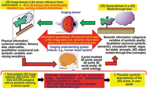
Figure 21. An observation (true-fact) familiar to all human beings wearing sunglasses, such as “spatial information dominates color information in vision” (Baraldi, 2017; Baraldi et al., 2018a, 2018b; Baraldi & Tiede, 2018a, 2018b), is typically questioned or disagreed upon by many computer vision (CV) and remote sensing (RS) experts and/or practitioners. At right, a panchromatic Baboon is as easy to be visually identified as such as its chromatic counterpart, at left, by any human photointerpreter. This perceptual fact works as proof-of-concept that the bulk of visual information is spatial rather than colorimetric in both the 4D geospace-time scene-domain and its projected (2D) image-plane. In spite of this unequivocal true-fact, to date, the great majority of the CV and RS communities adopt 1D non-retinotopic/2D spatial topology non-preserving (Baraldi, 2017; Baraldi & Alpaydin, 2002a, 2002b; Fritzke, 1997; Martinetz et al., 1994; Öğmen & Herzog, 2010; Tsotsos, 1990) image analysis algorithms, either pixel-based or local window-based, insensitive to permutations in the input data sequence (Cimpoi et al., 2014; Krizhevsky et al., 2012), where inter-object spatial topological relationships (e.g. adjacency, inclusion, etc.) and inter-object spatial non-topological relationships (e.g. spatial distance and angle measure) are oversighted in the (2D) image-plane (refer to Subsection 3.3.4), also refer to Figure 22.

Figure 22. Examples of 1D image analysis approaches (Baraldi, 2017; Baraldi et al., 2018a, 2018b; Baraldi & Tiede, 2018a, 2018b; Matsuyama & Hwang, 1990), 2D spatial topology non-preserving (non-retinotopic) in the (2D) image-domain (Baraldi, 2017; Baraldi & Alpaydin, 2002a, 2002b; Fritzke, 1997; Martinetz et al., 1994; Öğmen & Herzog, 2010; Tsotsos, 1990). Intuitively, 1D image analysis is insensitive to permutations in the input data set (Cimpoi et al., 2014; Krizhevsky et al., 2012). Synonym for 1D analysis of a 2D gridded data set, non-retinotopic 1D image analysis is affected by spatial data dimensionality reduction, from 2D to 1D. The (2D) image at top/left is transformed into the 1D vector data stream (sequence) shown at bottom/right, where vector data are either pixel-based (2D spatial context-insensitive) or spatial context-sensitive, e.g. local window-based or image-object-based. This 1D vector data stream means nothing to a human photo interpreter. When it is input to either an inductive learning-from-data classifier or a deductive learning-by-rule classifier, the 1D vector data sequence is what the classifier actually sees when watching the (2D) image at left. Undoubtedly, computers are more successful than humans in 1D image analysis. Nonetheless, humans are still far more successful than computers in 2D image analysis, which is 2D spatial context-sensitive and 2D spatial topology-preserving (retinotopic) (Baraldi, 2017; Baraldi & Alpaydin, 2002a, 2002b; Fritzke, 1997; Martinetz et al., 1994; Öğmen & Herzog, 2010; Tsotsos, 1990), see Figure 23. (a) Pixel-based (2D spatial context-insensitive) or (spatial context-sensitive) local window-based 1D image analysis. (b) Typical example of 1D image analysis approach implemented within the (geographic) object-based image analysis (GEOBIA) paradigm (Baraldi, Lang, Tiede, & Blaschke, 2018; Blaschke et al., 2014). In the so-called (GE)OBIA approach to CV, spatial analysis of (2D) imagery is intended to replace traditional pixel-based/2D spatial context-insensitive image analysis algorithms, dominating the RS literature to date. In practice, (GE)OBIA solutions can pursue either (2D spatial topology non-preserving, non-retinotopic) 1D image analysis or (2D spatial topology preserving, retinotopic) 2D image analysis (Baraldi et al., 2018). Also refer to Figures 23 and 24.

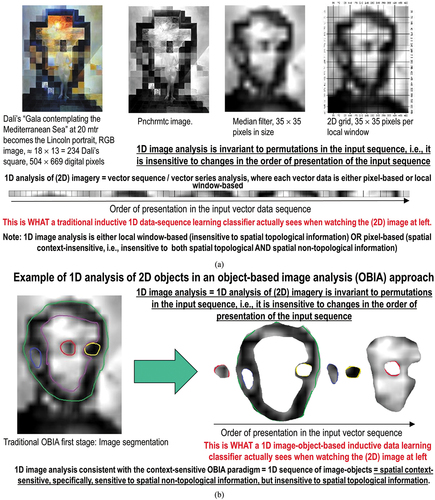
These considerations are obvious (unequivocal), but not trivial. De facto, they are in contrast with the RS common practice, where traditional general-purpose ‘ML → ANI → AGI’ solutions, suitable for coping with a 1D vector data sequence as input, such as the multi-layer perceptron, support vector machine, random forest, etc. (Bishop, 1995; Cherkassky & Mulier, 1998; Sonka et al., 1994), are widely adopted for ‘CV ⊃ EO-IU ⊃ ARD’ tasks.

Since they require as input a 1D vector data sequence, traditional inductive ‘ML → ANI → AGI’ algorithms are inherently unfitted to deal with input (2D) imagery, due to input data dimensionality reduction from 2D to 1D, either 1D pixel-based (2D spatial context-insensitive) or 1D local window-based, which causes a total or partial loss of the 2D spatial topological information component of (2D) imagery, see Figure 21 to Figure 23. In other words, if employed in 2D gridded data (image) mapping tasks, these traditional ML algorithms are 2D spatial topology non-preserving, i.e. they are non-retinotopic (Öğmen & Herzog, 2010; Tsotsos, 1990), in contrast with biological vision systems (refer to references listed in Section 2). Intuitively, any 1D image analysis algorithm, which is non-retinotopic, i.e. 2D spatial topology non-preserving (Baraldi, 2017; Baraldi & Alpaydin, 2002a, 2002b; Fritzke, 1997; Martinetz et al., 1994; Öğmen & Herzog, 2010; Tsotsos, 1990), is insensitive to permutations in the input data sequence (Cimpoi et al., 2014; Krizhevsky et al., 2012).

Figure 23. Alternative to 1D analysis of (2D) imagery (see .Figure 22), 2D image analysis (Baraldi, 2017; Baraldi et al., 2018a, 2018b; Baraldi & Tiede, 2018a, 2018b; DiCarlo, 2017; Öğmen & Herzog, 2010; Tsotsos, 1990) is synonym for 2D analysis of (2D) imagery, meaning 2D spatial context-sensitive and 2D spatial topology-preserving (retinotopic) feature mapping in a (2D) image-domain (Baraldi, 2017; Baraldi & Alpaydin, 2002a, 2002b; Fritzke, 1997; Martinetz et al., 1994; Öğmen & Herzog, 2010; Tsotsos, 1990). Intuitively, 2D image analysis is sensitive to permutations in the input data set (Cimpoi et al., 2014; Krizhevsky et al., 2012). Activation domains of physically adjacent processing units in the 2D array (grid, network) of 2D convolutional spatial filters are spatially adjacent regions in the 2D visual field (image-plane). Distributed processing systems capable of 2D image analysis, such as physical model-based (‘handcrafted’) 2D wavelet filter banks (Baraldi, 2017; Burt & Adelson, 1983; DiCarlo, 2017; Jain & Healey, 1998; Mallat, 2009; Marr, 1982; Sonka et al., 1994), typically provided with a high degree of biological plausibility in modelling 2D spatial topological and spatial non-topological information components (DiCarlo, 2017; Heitger et al., 1992; Kosslyn, 1994; Mason & Kandel, 1991; Öğmen & Herzog, 2010; Rappe, 2018; Rodrigues & Du Buf, 2009; Slotnick et al., 2005; Tsotsos, 1990; Vecera & Farah, 1997) and/or deep convolutional neural networks (DCNNs), typically learned inductively (bottom-up) from data end-to-end (Cimpoi et al., 2014; Krizhevsky et al., 2012), are eligible for outperforming traditional 1D image analysis approaches. Will computer vision (CV) systems ever become as good as humans in 2D image analysis? Also refer to Figure 24. Unfortunately, due to bad practices in multi-scale spatial filtering implementation (Geirhos et al., 2018; Zhang, 2019), modern inductive DCNN algorithms typically neglect the spatial ordering of object parts, i.e. they are insensitive to the shuffling of image parts (Brendel, 2019; Brendel & Bethge, 2019). In practice, large portions of modern inductive DCNNs adopt a decision-strategy very similar to that of traditional 1D image analysis approaches, such as bag-of-local-features models (Brendel, 2019; Brendel & Bethge, 2019), insensitive to permutations in the 1D sequence of input data (Bourdakos, 2017), see Figure 25.

Provided with a relevant survey value, the present Section critically reviews the multi-disciplinary domain of the cognitive task of vision, synonym for inherently ill-posed 4D scene-from-(2D) image reconstruction and understanding (see Figure 20), encompassing both biological vision and CV, where semantic relationship ‘EO-IU ⊂ CV ⊂ AGI ⊂ Cognitive science’ = Equation (3)(3) $\text{lsquo}\mathrm{A}\mathrm{R}\mathrm{D}\subset \mathrm{E}\mathrm{O}-\mathrm{I}\mathrm{U}\subset \mathrm{C}\mathrm{V}\subset \mathrm{A}\mathrm{G}\mathrm{I}\subset \mathrm{C}\mathrm{o}\mathrm{g}\mathrm{n}\mathrm{i}\mathrm{t}\mathrm{i}\mathrm{v}\mathrm{e}\mathrm{s}\mathrm{c}\mathrm{i}\mathrm{e}\mathrm{n}\mathrm{c}\mathrm{e}\text{rsquo}$(3) holds, meaning that ‘CV ⊃ EO-IU’ cognitive systems are regarded as subset-of (specialization-of, with inheritance) inherently ill-posed AGI system solutions (refer to Subsection 3.5). Knowledge on inherently ill-posed ‘EO-IU ⊂ CV ⊂ AGI’ cognitive systems, capable of qualitative/equivocal information-as-data-interpretation, is regarded as background knowledge of the RS meta-science (Couclelis, 2012), whose overarching goal is to transform multi-source EO large image databases into VAPS in operational mode (refer to Subsection 3.1), in compliance with a new notion of Space Economy 4.0 (Mazzucato & Robinson, 2017), suitable for coping with grand societal challenges, such as the UN SDGs from year 2015 to 2030 (UN – United Nations, Department of Economic and Social Affairs, 2021) (refer to Section 2).

In this Section, first, a critical review of the multi-disciplinary literature on the cognitive task of vision is proposed. Next, a set of Bayesian inference constraints is presented to better condition inherently ill-posed ‘CV ⊃ EO-IU ⊃ ARD’ system solutions, in agreement with a Bayesian/ driven-by-prior-knowledge/ class-conditional approach to data analysis (Bowers & Davis, 2012; Ghahramani, 2011; Lähteenlahti, 2021; Quinlan, 2012; Sarkar, 2018). Since semantic relationship ‘EO-IU ⊂ CV ⊂ AGI’ = Equation (3)(3) $\text{lsquo}\mathrm{A}\mathrm{R}\mathrm{D}\subset \mathrm{E}\mathrm{O}-\mathrm{I}\mathrm{U}\subset \mathrm{C}\mathrm{V}\subset \mathrm{A}\mathrm{G}\mathrm{I}\subset \mathrm{C}\mathrm{o}\mathrm{g}\mathrm{n}\mathrm{i}\mathrm{t}\mathrm{i}\mathrm{v}\mathrm{e}\mathrm{s}\mathrm{c}\mathrm{i}\mathrm{e}\mathrm{n}\mathrm{c}\mathrm{e}\text{rsquo}$(3) holds, i.e. ‘CV ⊃ EO-IU’ is a special case of (subset-of, with inheritance) AGI, then, in agreement with a stepwise approach, a set of Bayesian constraints proposed to better condition inherently ill-posed ‘CV ⊃ EO-IU’ systems is expected to be more severe (specialized, domain-specific) than the general-purpose set of constraints proposed for AGI solutions in Subsection 3.5.

4.1. Critical review of the multi-disciplinary literature on the cognitive task of vision, encompassing both biological vision and CV

Synonym for 4D geospace-time scene-from-(2D) image reconstruction and understanding (Matsuyama & Hwang, 1990) (refer to Section 2), vision is a cognitive task (process), pertaining to the multi-disciplinary domain of cognitive science (refer to references listed in Section 2) (see Figure 11), i.e. vision is an inherently ill-posed/ qualitative/ equivocal information-as-data-interpretation problem (Capurro & Hjørland, 2003) (refer to Subsection 3.3.3), see Figure 20. Encompassing both biological vision and CV, where CV belongs to semantic relationship ‘Cognitive science ⊃ AGI ⊃ CV ⊃ EO-IU ⊃ ARD’ = Equation (3)(3) $\text{lsquo}\mathrm{A}\mathrm{R}\mathrm{D}\subset \mathrm{E}\mathrm{O}-\mathrm{I}\mathrm{U}\subset \mathrm{C}\mathrm{V}\subset \mathrm{A}\mathrm{G}\mathrm{I}\subset \mathrm{C}\mathrm{o}\mathrm{g}\mathrm{n}\mathrm{i}\mathrm{t}\mathrm{i}\mathrm{v}\mathrm{e}\mathrm{s}\mathrm{c}\mathrm{i}\mathrm{e}\mathrm{n}\mathrm{c}\mathrm{e}\text{rsquo}$(3) , vision is very difficult to solve because:

1. Non-deterministic polynomial (NP)-hard in computational complexity (Frintrop, 2011; Tsotsos, 1990). And

2. Inherently ill-posed in the Hadamard sense (Baraldi, 2017; Baraldi et al., 2018a, 2018b; Baraldi & Tiede, 2018a, 2018b; Marr, 1982; Matsuyama & Hwang, 1990; Quinlan, 2012), i.e. vision admits no solution, multiple solutions or, if the solution exists, the solution’s behavior changes continuously with the initial conditions (Hadamard, 1902) (refer to Section 2). Vision is inherently ill-posed in the Hadamard sense because affected by:

   1. A 4D-to-2D data dimensionality reduction, from the 4D geospatio-temporal scene-domain to the (2D, planar) image-domain (image-plane), which is responsible of occlusion phenomena, see Figure 20. And

   2. A semantic information gap (Matsuyama & Hwang, 1990), from ever-varying subsymbolic sensory data (sensations) in the (2D) image-plane to stable symbolic percepts in the mental model of the physical world (modeled world, world ontology, real-world model) (refer to Subsection 3.3.4), see Figure 20.

A first unequivocal fact (true-fact, observation) about the cognitive task of vision is that, since it is inherently ill-posed, vision (encompassing both biological vision and CV) requires a priori knowledge, available in addition to sensory 2D gridded data (imagery) (Baraldi, 2017; Van der Meer & De Jong, 2011; Victor, 1994), to become better conditioned for numerical solution (Baraldi, 2017; Baraldi et al., 2018a, 2018b; Baraldi & Tiede, 2018a, 2018b; Bishop, 1995; Cherkassky & Mulier, 1998; Dubey et al., 2018).

Considered mandatory to make the inherently ill-posed cognitive (information-as-data-interpretation) task of vision better conditioned for numerical solution, a priori visual knowledge, known as Marr’s constraints (Marr, 1982; Quinlan, 2012), must be encoded by design in the visual system, in agreement with a Bayesian inference approach (Bowers & Davis, 2012; Ghahramani, 2011; Lähteenlahti, 2021; Quinlan, 2012; Sarkar, 2018) to scene-from-image reconstruction and understanding tasks (Marr, 1982), see Figure 11(a).

By definition, a priori knowledge, if any, is available in addition to sensory data (it is available before looking at data, before collecting observations), i.e. prior knowledge is never alternative to data/observation. In agreement with a Bayesian inference paradigm (refer to references listed above in this Subsection), prior knowledge works as initial conditions. For example, according to genetic epistemology, in biological cognitive systems, “there is never an absolute beginning” (Piaget, 1970), because learning-from-examples phenotype starts exploring a solution space from initial conditions provided by a genotype, available a priori (Baraldi, 2017; Parisi, 1991; Zador, 2019) (refer to Subsection 3.3.4).

Stemming from these first principles, it is straightforward to speculate that vision is a hybrid inference process, combining deductive/ top-down/ driven-by-prior knowledge inference with inductive/ bottom-up/ driven-by-data inference, to take advantage of each and overcome their shortcomings (refer to Subsection 3.3.2). For example, Vecera and Farah wrote: “we have demonstrated that (low-level, pre-attentional) image segmentation [as the dual problem of image-contour detection] is inherently ill-posed [in the Hadamard sense]. It can be influenced by the familiarity of the shape being segmented … these results are consistent with the hypothesis that image segmentation is an interactive [hybrid inference] process … in which top-down knowledge partly guides lower level processing” (Vecera & Farah, 1997).

The abovementioned quote from (Vecera & Farah, 1997) fully complies with additional evidence in neuroscience, where “mental imagery is known to induce retinotopically organized activation of early (retinal) visual areas via feedback connections” (Hawkins, 2021; Hawkins et al., 2017), which is tantamount to saying that “mental images in the mind’s eye can alter the way we see things in the retina” (Slotnick et al., 2005). Additional recent studies in visual science suggest that, in a sense, “mammals dream about the world they are about to experience before they are even born. Waves of activity that emanate from the neonatal retina in mice before their eyes ever open disappear soon after birth and are replaced by a more mature network of neural transmissions of visual stimuli to the brain, where information is further encoded and stored. At eye opening, mammals are capable of pretty sophisticated perception of motion and behaviors to navigate the world because, before their eyes opened, their retinal waves flow in a pattern that mimics the activity that would occur if the mammal were moving forward through the environment” (Hathaway, 2021).

In agreement with quotes in visual science reported above (Hathaway, 2021; Hawkins, 2021; Hawkins et al., 2017; Slotnick et al., 2005; Vecera & Farah, 1997), it is straightforward to observe that, in the cognitive/mental process of vision, whereas sensory data (sensations) collected by an imaging sensor (eye), by means of forward (sensor-to-mind) mapping of an observed 4D geospace-time scene-domain onto a (2D) image-plane (retina), are ever-varying (see Figure 20), stable/hard-to-vary (Sweeney, 2018a) information/ knowledge/ constraints can be mapped backward (back-projected, mind-to-sensor) (Hathaway, 2021; Hawkins, 2021; Hawkins et al., 2017; Kosslyn, 1994; Matsuyama & Hwang, 1990; Slotnick et al., 2005), via directed feedback connections, from the high-level inference system (mind), accounting for the mind-brain problem (Serra & Zanarini, 1990; Westphal, 2016) (refer to Section 2) and provided with a 7D stable/hard-to-vary conceptual model of the world in user-speak (refer to Section 2), consisting of stable percepts (Matsuyama & Hwang, 1990), such as entities/referents (Ball, 2021) and inter-entity relationships/predicates (Ball, 2021) (refer to Subsection 3.3.4), onto the low-level (2D) image-plane.

Both forward sensor-to-mind connections and backward mind-to-sensor connections (see Figure 20) are modulated by (filtered by) a stable/hard-to-vary set of imaging sensor-specific (eye-specific) characteristics, in techno-speak, see Figure 8. For example, in the 7D domain of the conceptual world model in user-speak (refer to Section 2), popular units of measure are meter for distance and second for time (Matsuyama & Hwang, 1990). In the difficult (non-intuitive) technical terms of a techno-speak, imaging sensor properties are spatial resolution, spectral resolution, temporal resolution, etc. (see Figure 8), where pixel is the spatial unit of measure in the (2D) image-plane (Matsuyama & Hwang, 1990).

Noteworthy, a conceptual/ mental/ perceptual world model of stable/hard-to-vary entities and relationships in user-speak exists independently of an imaging sensor in techno-speak. In other words, pertaining to the domain of a priori knowledge, a stable/hard-to-vary conceptual world model exists, whether or not an imaging sensor is observing the world. For example, in a stable sensor-independent mental world model, LC class cars exists, whether or not cars can be detected in ever-varying observations (sensory data) of the world, such as spaceborne EO imagery.

Like a mental world model is stable/hard-to-vary and pertains to prior knowledge (like genotype), available in addition to sensory data, so is an imaging sensor specification, typically known before image acquisition, see Figure 8. However, unlike the conceptual world model in user-speak, imaging sensor properties are in techno-speak. For example, sensor-specific spatial, spectral and temporal resolutions in techno-speak (see Figure 8) are hyperparameters to be encoded by design in a CV system.

As an example of CV system where a mental world model in user-speak and an imaging sensor model in techno-speak are both available as a priori knowledge, let us consider a 7D conceptual world model (refer to Subsection 3.3.4) where LC class cars exists in the LC class vocabulary and features as attribute of size in length in the world-domain the physical range of change from 2 to 7 meters in user-speak. If the imaging sensor’s spatial resolution is 30 meter per pixel in a sensor-specific techno-speak, then the mind-to-sensor feedback projection infers, based on prior knowledge exclusively, that no instance of LC class cars can ever be detected for recognition in the image-plane of that imaging sensor.

On the contrary, if it is known a priori that the imaging sensor’s spatial resolution is 0.5 meter per pixel and the optical imaging sensor is achromatic (panchromatic, PAN, refer to Section 2), then the mind-to-sensor feedback projection figures, based on prior knowledge exclusively, that an instance of LC class cars can be detected in the image-plane if an image-object’s size in length belongs to range 4 to 14 in pixel units in the sensor-specific techno-speak, whereas no real-world car’s colorimetric property can be exploited for panchromatic visual detection and recognition of instances of LC class cars, according to a convergence of spatial evidence with color evidence approach, i.e. spatial evidence in the image-plane must suffice for real-world object detection and recognition in PAN image interpretation, see Figure 21.

In the cognitive science subdomain of ‘AGI ⊃ CV ⊃ EO-IU ⊃ ARD’ problems, the mind-to-sensor back-projection of a stable/hard-to-vary and sensor-independent 7D conceptual/ mental/ perceptual world model in user-speak onto a (2D) image-plane through a known and stable, but sensor-specific, imaging sensor parameterization in techno-speak (see Figure 8), typical of biological vision as described in the previous paragraphs, becomes an example of top-down knowledge transfer, from human-to-machine (Laurini & Thompson, 1992). In traditional expert systems, also referred to as GOFAI (Dreyfus, 1965, 1991, 1992; Santoro et al., 2021) (see Figure 11), top-down knowledge transfer from human-to-machine is accomplished by knowledge engineering (Laurini & Thompson, 1992; Sowa, 2000). Aiming at solving practical problems in-the-world within given constraints of budgets and deadlines (Sowa, 2000, p. 132), knowledge engineering is the process of codifying knowledge in the user-speak, L, of human experts about some world-domain, D, into a computable model in techno-speak, e.g. in data structures combined with a static (non-adaptive to data) if-then prior knowledge-based rule set in a GOFAI framework (Laurini & Thompson, 1992, p. 641) (refer to Subsection 3.3.4).

By analogy with traditional expert systems, in CV applications, the role of knowledge engineering would be to encode in techno-speak (e.g. in data structures), first, a stable/hard-to-vary 7D conceptual world model collected in user-speak from world-domain human experts (refer to Subsection 3.3.4). Once a stable/hard-to-vary and sensor-independent 7D conceptual/ mental/ perceptual world model in user-speak has been structured and encoded in techno-speak by knowledge engineers, e.g. in the graphical techno-speak of a semantic network or Petri net which is easier to be shared to be community-agreed upon (refer to Subsection 3.3.4), then, via directed feedback (mind-to-sensor) connections, a conceptual world model, now encoded in techno-speak, can be modulated by (filtered by) an imaging sensor-specific model, which is also in techno speak, if the imaging sensor specifications (e.g. spatial, spectral and temporal resolutions) are also known a priori (see Figure 8), in addition to the stable/hard-to-vary conceptual world model.

To recap, in the cognitive science subdomain of inherently ill-posed ‘AGI ⊃ CV ⊃ EO-IU ⊃ ARD’ problems (see Figure 20), where a priori knowledge is mandatory in addition to imagery to make the inherently ill-posed cognitive problem of 4D geospace-time scene-from-(2D) image reconstruction and understanding better conditioned for numerical solution (refer to references listed in this Subsection above), there are two sources of a priori knowledge, available in addition to imagery. First, the imaging sensor technical specifications, in techno-speak, are typically known in advance, before image acquisition, see Figure 8. Second, a 7D conceptual/ mental/ perceptual world model is available in human-speak, to be community-agreed upon. The latter requires knowledge engineering (Laurini & Thompson, 1992, p. 641) to be transcoded from human-speak into techno-speak, e.g. the graphical techno-speak of a Petri net. Hence, in CV applications, knowledge engineering is mandatory to accomplish top-down knowledge transfer (Laurini & Thompson, 1992), from human (being-in-the-world, which includes their mental model of the world) to machine (whose being is not in the physical world of humans) (Capurro & Hjørland, 2003; Dreyfus, 1965, 1991, 1992; Fjelland, 2020) (refer to Section 2).

Unfortunately, the CV and the RS common practice are very different from the conceptual and methodological scenario described above in the multi-disciplinary domain of cognitive science, where top-down knowledge transfer, from human (being-in-the-world) to machine (whose being is not in the physical world of humans), is mandatory and requires knowledge engineering to be accomplished (Laurini & Thompson, 1992; Sowa, 2000).

For example, in (Belgiu, Drǎguţ, & Strobl, 2014), the research goal was to quantitatively assess the robustness to changes in input data of a second-stage static (non-adaptive to data) prior spectral knowledge-based decision-tree classifier, typically adopted in sequence to a semi-automatic inductive learning-from-data algorithm for MS image segmentation (partitioning), in agreement with a two-stage hybrid (in this case, combined first-stage inductive and second-stage deductive) geographic object-based image analysis (GEOBIA) paradigm (Baraldi et al., 2018; Blaschke et al., 2014), see Figure 24. One prior spectral knowledge-based decision-tree classifier was designed and implemented independently by each of the three authors to detect four target LC classes, specifically, impervious surface, bare soil, vegetation and water (which are located across the three hierarchical dichotomous layers of the standard FAO LCCS-DP taxonomy, see Figure 3) in a toy problem, regarding two test areas, one test area of 3556 × 2521 pixels in size, the second test area of larger extent, 7328 × 4181 pixels in size, covering 90% of the first test site, within the same very high resolution spaceborne EO image acquired by the WorldView-2 imaging sensor, featuring eight spectral channels, ranging from the visible Blue to the Near InfraRed (NIR) portion of the electromagnetic spectrum, with spatial resolution equal to 2 m.

Figure 24. A (geographic) object-based image analysis (GEOBIA) paradigm (Blaschke et al., 2014), reconsidered (Baraldi et al., 2018). In the (GE)OBIA subdomain of computer vision (CV) (see Figure 11), spatial analysis of (2D) imagery is intended to replace traditional pixel-based (2D spatial context-insensitive) image analysis algorithms, dominating the remote sensing (RS) literature and common practice to date. In practice, (GE)OBIA solutions encompass either 1D image analysis (spatial topology non-preserving, non-retinotopic) or 2D image analysis (spatial topology preserving, retinotopic). To overcome limitations of the existing GEOBIA paradigm (Blaschke et al., 2014), in a more restrictive definition of EO for Geographic Information Science (GIScience) (EO4GIScience) (see Figure 11), novel EO4GIScience applications consider mandatory a 2D image analysis approach, see Figure 23 (Baraldi et al., 2018).

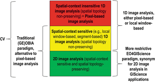
A first critical observation about this experimental setting is that, to fairly assess and compare robustness to changes in input data, the three static (non-adaptive to data) prior spectral knowledge-based decision-tree classifier implementations under comparison adopt as input the same sets of image-segments and segment-based (per-segment) secondary (subordinate in relevance, see Figure 21) spectral features, but ignore per-segment geometric (shape) and size properties together with inter-segment primary (dominant in relevance, see Figure 21) 2D spatial topological and 2D spatial non-topological relationships, in the arguable pursuit of a 2D spatial topology non-preserving/non-retinotopic 1D image analysis approach to the GEOBIA paradigm, see Figure 22(b) and Figure 24.

A second critical observation is that, in (Belgiu et al., 2014), enigmatically, but not surprisingly in the context of bad practices affecting the RS community (refer to Subsection 3.5), at the EO data pre-processing stage, preliminary to EO data analysis, in spite of their quest for system robustness, the three authors totally ignore EO data radiometric Cal requirements (refer to Subsection 3.5), considered mandatory to provide dimensionless EO sensory data with a physical meaning, eligible for EO radiometrically calibrated data to become better behaved and better understood than their uncalibrated counterparts, in compliance with an intuitive GIGO principle (Baraldi, 2017; Geiger et al., 2021; Thompson, 2018), with the popular FAIR criteria for scientific data (product and process) management (GO FAIR – International Support and Coordination Office, 2021; Wilkinson et al., 2016) (see Table 1) and with the intergovernmental GEO-CEOS QA4EO Cal requirements (refer to references listed in Section 2).

After testing for robustness to changes in input data their three deductive prior spectral knowledge-based decision-tree classification algorithms in a toy data interpretation problem, consisting of two small and overlapping test areas in a single EO image where no radiometric Cal data pre-processing is adopted to augment data harmonization/interoperability, these authors concluded that “[the three prior spectral knowledge-based] object-based decision-tree classifications remain consistent to a certain degree when applied to other test areas”.

Rather than a helpful conclusion, this final statement is a typical example of non-informative tautology (an expression in which the same thing is said twice in different words). It is indeed a contradiction in terms to assess whether a static prior knowledge-based decision tree, implemented to work in a (WorldView-2) imaging sensor-specific image-plane as back-projection of an a priori sensor-independent stable conceptual/ mental/ perceptual world model (e.g. in this experiment, the conceptual world model is agreed-upon by the community of the three authors and comprises as entities four target LC classes located across the three hierarchical dichotomous layers of the standard FAO LCCS-DP taxonomy, see Figure 3), filtered/modulated by the imaging sensor-specific technical specifications known a priori (e.g. in this experiment, only the spectral resolution and the spatial resolution of the WorldView-2 imaging sensor are relevant, since temporal resolution is irrelevant for the single-date image interpretation task at hand, see Figure 8), is robust to changes in input data representative of the complexity of real-world problems (refer to Subsection 3.1), which includes changes in sensor specifications and excludes toy problems at small spatial extents, such as the experimental problem at hand.

In spite of reaching non-informative conclusions about a CV toy problem, whose specifications encompass few target LC classes at coarse levels of semantics (see Figure 3), a single imaging sensor, a single image acquired by that sensor and two small and overlapping test areas within a single input image, these three authors actually brought to surface a relevant cognitive fact, pertaining to the multi-disciplinary domain of cognitive science: while coping with the same oversimplistic problem (toy problem, not representative of the complexity of real-world problems), pertaining to the CV subdomain of cognitive science (see Figure 11), three human experts, who shared the same a priori conceptual world model in human-speak and the same a priori imaging sensor specifications in techno-speak, ended up with three different implementations of a prior knowledge-based CV (expert, static decision-tree) system.

In more detail, in (Belgiu, Drǎguţ, and Strobl, 2014), the three authors proved that their individual mind-to-sensor backward knowledge mapping is inherently ill-posed and, therefore, very difficult to solve (refer to Section 2). Mind-to-sensor backward knowledge mapping consists of two steps. First, a conceptual world model in user-speak is community-agreed upon and translated into techno-speak by knowledge engineering. For example, at this phase, in this experiment, inter-entity relationships are ignored in a semantic network where the conceptual world model is represented graphically in techno-speak (refer to Subsection 3.3.4). Second, the a priori world model transformed into techno-speak by knowledge engineering is filtered by/ modulated by/ mapped through the imaging sensor-dependent spatial, spectral and temporal specifications, known a priori in techno-speak (see Figure 8), to be (mind-to-sensor) back-projected onto a (WorldView-2) sensor-specific (2D) image-plane in techno-speak, where, for example, the spatial unit of measure is pixel.

Our conclusion, learned from the (cognitive) experiment proposed in (Belgiu, Drǎguţ, and Strobl, 2014), is that knowledge engineering is “AGI-complete” (Saba, 2020c; Wikipedia, 2021a). It is, per se, a cognitive (sub)problem (refer to Section 2), inherently ill-posed in the Hadamard sense (Baraldi, 2017; Baraldi and Tiede, 2018a; Baraldi and Tiede, 2018b; Hadamard, 1902; Matsuyama and Hwang, 1990). Hence, it is very difficult to solve (Frintrop, 2011; Tsotsos, 1990).

Back to the inherently ill-posed cognitive task of vision, encompassing both biological vision and CV (see Figure 20), a second unequivocal fact (true-fact, observation) is that, in biological vision, spatial information typically dominates color information (Baraldi, 2017; Baraldi et al., 2018a, 2018b; Baraldi & Tiede, 2018a, 2018b), see Figure 21. This inference stems from the observation (true-fact) that, in human visual perception, achromatic/panchromatic (PAN) and chromatic visions are nearly as effective in scene-from-image reconstruction and understanding (Baraldi, 2017; Baraldi & Tiede, 2018a, 2018b), see Figure 21.

Noteworthy, the observation that, in biological vision, spatial information typically dominates colorimetric information means that this information property holds true in both the observed 4D geospace-time scene-domain and in the projected (2D) image-plane (Baraldi, 2017; Baraldi & Tiede, 2018a, 2018b), since both spatial domains, the 3D geospace scene-domain and the (2D) image-domain, are involved with the cognitive task of vision, see Figure 20.

The observation that, in biological vision, spatial information typically dominates color information is obvious (unequivocal) per se, but not trivial. This perceptual evidence is familiar to all human beings wearing sunglasses. In spite of being experienced by humans in their daily visual practice, when asked if spatial information dominates colorimetric information in vision, many CV and RS experts and/or practitioners typically remain puzzled before typically answering: no, at least at first round. This attentional (conscious) denial of a pre-attentional (unconscious) visual evidence proves the ongoing lack of (attentional, conscious) knowledge in cognitive science (Langley, 2012), with special emphasis on biological vision and psychophysics (see Figure 11), affecting large portions of the CV and RS meta-science communities working with the cognitive task of vision (image interpretation) at a professional level (Couclelis, 2012) (also refer to Appendix I). In practice, many scientists dealing with CV problems have little or no background (prior) knowledge in the cross-disciplinary domains of biological visual machinery (brain) and perception (mental interpretation/understanding of sensory data) (DiCarlo, 2017; Dubey et al., 2018; Heitger et al., 1992; Iqbal & Aggarwal, 2001; Kosslyn, 1994; Marr, 1982; Mason & Kandel, 1991; Mély et al., 2018; Öğmen & Herzog, 2010; Perez, 2017, 2018; Pessoa, 1996; Rappe, 2018; Rodrigues & Du Buf, 2009; Slotnick et al., 2005; Tsotsos, 1990; Vecera & Farah, 1997). In the words of Qasim Iqbal and Jagdishkumar Aggarwal “frequently, no claim is made about the pertinence or adequacy of the digital models as embodied by computer algorithms to the proper model of human visual perception … This enigmatic situation arises because RTD in CV is often considered quite separate from research into the functioning of human vision. A fact that is generally ignored is that biological vision is currently the only measure of the incompleteness of the current stage of computer vision, which illustrates that the problem is still open to solution” (Iqbal & Aggarwal, 2001).

In line with the aforementioned observation stemming from human visual perception, postulate ‘DL ⊂ ML → ANI → AGI ⊃ CV ← Human vision’ = Equation (4)(4) $\begin{array}{rl}& \text{lsquo}(Inductive/bottom\text{-}up/statisticalmodel\text{-}based)DL\text{-}from\text{-}data\subset \\ & (Inductive/bottom\text{-}up/statisticalmodel\text{-}based)ML\text{-}from\text{-}data\\ & \to AGI\supset CV\leftarrow Humanvision\text{rsquo}\end{array}$(4) holds, see Figure 11(a). This working hypothesis means that, to become better constrained for numerical solution (refer to references listed in this Subsection above), inherently ill-posed ‘CV ⊃ EO-IU ⊃ ARD’ systems are required to incorporate by design a computational model of human vision, in compliance with human visual perception, as lower bound. In contrast with the ongoing “enigmatic situation” where RTD in ‘EO-IU ⊂ CV ⊂ AGI’ is “considered quite separate from research into the functioning of human vision and visual perception” (Iqbal & Aggarwal, 2001), Equation (4)(4) $\begin{array}{rl}& \text{lsquo}(Inductive/bottom\text{-}up/statisticalmodel\text{-}based)DL\text{-}from\text{-}data\subset \\ & (Inductive/bottom\text{-}up/statisticalmodel\text{-}based)ML\text{-}from\text{-}data\\ & \to AGI\supset CV\leftarrow Humanvision\text{rsquo}\end{array}$(4) adopted herein as axiom urges the multi-disciplinary cognitive science community to provide meta-sciences, like engineering, computer science, CV and RS (Couclelis, 2012), with a broad education in AGI that “cuts across different topics to cover all the field’s branches and their role in intelligent systems … (such as) cognitive psychology, linguistics, and logic, which are far more important to the cognitive systems agenda than ones from mainstream computer science” (Langley, 2012) (refer to Appendix I).

The primary relevance of spatial information in the 4D geospatio-temporal physical world is acknowledged by GIScience (refer to references listed in Section 2), where the Tobler’s first law (TFL) of geography (Tobler, 1970), familiar to all geographers, states that “all things are related, but nearby things are more related than distant things”, although certain phenomena clearly constitute exceptions (Longley et al., 2005). Unfortunately, the quantitative counterpart of the qualitative TFL of geography, specifically, the statistical concept of spatial autocorrelation (Baraldi, 2017; Wikipedia, 2014a, 2014b) remains obscure to many geographers.

At the same time, the statistical concept of spatial autocorrelation in imagery (2D gridded data set) (Baraldi, 2017; Geirhos et al., 2018; Jain & Healey, 1998; Julesz, 1986; Julesz, Gilbert, Shepp, & Frisch, 1973; Victor, 1994; Wikipedia, 2014a, 2014b; Yellott, 1993), pertaining to the image-domain in the cognitive process of vision (see Figure 20), remains apparently obscure to many CV and RS experts and practitioners, such as those involved with the development or exploitation of low-level image segmentation/partitioning algorithms (Baatz & Schäpe, 2000; Camara, Souza, Freitas, & Garrido, 1996; Espindola, Camara, Reis, Bins, & Monteiro, 2006), typically adopted as first stage in the (GE)OBIA paradigm, see Figure 24. For example, the Yellott Triple spatial-autocorrelation uniqueness theorem, stating that every panchromatic (one-channel multi-gray leveled) image of finite size is uniquely determined (up to spatial translation) by its image-wide third-order statistics (Yellott, 1993), has been rarely investigated by the CV and RS communities (Baraldi, 2017).

In truth, the unquestionable relevance of spatial autocorrelation in both the 4D geospatio-temporal world-domain, typically investigated by GIScience, and the projected (2D) image-domain involved with the cognitive task of vision can be regarded as the true-fact (observation) at the origin of the development of the (GE)OBIA approach to CV, conceived around year 2000 by the GIScience community to overcome limitations of traditional 2D spatial-context insensitive/non-retinotopic 1D pixel-based image analysis algorithms (Blaschke et al., 2014), see Figure 22(a).

Unfortunately, whereas 2D spatial-context insensitive/1D pixel-based image analysis is inherently unsuitable for pursuing vision as synonym for (retinotopic) 2D spatial analysis of 2D gridded data (see Figure 24), the (GE)OBIA paradigm is not required to pursue 2D spatial topology-preserving analysis of (2D) imagery either, see Figure 23. As a consequence, typical (GE)OBIA algorithms are non-retinotopic (2D spatial topology non-preserving) too, see Figure 22(b). Moreover, typical (GE)OBIA algorithms are based on heuristics at the inherently ill-posed image segmentation first phase (Baatz & Schäpe, 2000; Camara et al., 1996; Espindola et al., 2006) and, as a consequence, they typically score (fuzzy) “low” in an mDMI set of OP-Q²Is (refer to Subsection 3.1), encompassing degree of automation (bottom-up/inductive image segmentation algorithms are typically semi-automatic, i.e. they require several empirical hyperparameters to be user-defined based on heuristics/trial-and-error), data mapping (image segmentation) accuracy (e.g. image segmentation algorithms are typically inconsistent with human visual perception in ramp-edge detection, in compliance with the Mach bands visual illusion phenomenon, see Figure 27), robustness to changes in input data (since they are based on heuristics, image segmentation algorithms typically score low in large and/or heterogeneous data sets, reflecting the complexity of real-world problems), etc. (refer to the farther Subsection 4.2).

Due to the ongoing lack of suitable alternatives, including (GE)OBIA, benefitting from its conceptual simplicity and implementation straightforwardness in raster graphics formats (refer to Section 2) and despite its total lack in analytics of dominant 2D spatial information, 2D spatial context-insensitive/1D pixel-based image analysis remains, to date, the predominant suboptimal approach to ‘CV ⊃ EO-IU ⊃ ARD’ system solutions, implemented for either low-level pre-processing (enhancement) or high-level analysis (interpretation) of multi-sensor EO big 2D gridded data (see Figure 18) by the RS community (DLR – Deutsches Zentrum für Luft-und Raumfahrt e.V. and VEGA Technologies, 2011; ESA – European Space Agency, 2015; Gómez-Chova et al., 2007; Gorelick et al., 2017; Lillesand & Kiefer, 1979; OHB, 2016; Picoli et al., 2018; Sonka et al., 1994; Swain & Davis, 1978; USGS – U.S. Geological Survey, 2018a, 2018b; Vermote & Saleous, 2007).

At the Marr level of system understanding 2-of-5, specifically, information/knowledge representation (refer to Subsection 3.2), in a CV system, the primary/dominant spatial information (see Figure 21) consists of several statistically independent (refer to Section 2) spatial information components in the 4D geospace-time scene-domain, which are projected by an imaging sensor onto a (2D) image-plane, see Figure 20. Statistically independent components of the primary/dominant spatial information in the 4D geospace-time scene-domain and in the projected (2D) image-plane of an imaging sensor (see Figure 20) are listed below (Baraldi, 2017).

• (Object-specific, per-object) geometric shape in a 4D geospace-time scene-domain. In the projected (2D, planar) image-domain, image-objects, also known as segments, regions, connected-components or tokens (Baraldi, 2017; Dillencourt, Samet, & Tamminen, 1992; Marr, 1982; Perona & Malik, 1990), typically investigated in the Gestalt laws of perceptual grouping (Cherry, 2019; Green, 1997; Koffka, 1935; Tuceryan, 1992), can be either 0D (pixel), 1D (line) or 2D (polygon), in agreement with the Open Geospatial Consortium (OGC) nomenclature (OGC – Open Geospatial Consortium Inc, 2015), to be parameterized by scale-invariant planar (2D) shape indexes (Baraldi, 2017; Baraldi & Soares, 2017).

• (Object-specific, per-object) size in a 4D geospace-time scene-domain. For example, in the scene-domain, size is expressed in user-speak (natural language) (Brinkworth, 1992), encompassing physical units of spatial distance, say, meter. In the projected (2D) image-domain, size is expressed in techno-speak (Brinkworth, 1992), where a spatial distance is in pixel units (Baraldi, 2017; Baraldi et al., 2018a, 2018b; Baraldi & Tiede, 2018a, 2018b; Matsuyama & Hwang, 1990).

• Inter-object 3D geospatial topological relationships, e.g. inclusion, adjacency, etc., in a 4D geospace-time scene-domain (Baraldi, 2017; Buyong, 2007; OGC – Open Geospatial Consortium Inc, 2015). In the projected (2D, planar) image-domain, 2D spatial topological relationships involve 0D, 1D or 2D image-objects (segments, regions, connected-components, tokens) (Baraldi, 2017; Dillencourt et al., 1992; Marr, 1982; Perona & Malik, 1990).

• Inter-object 3D geospatial non-topological relationships, e.g. distance-from, in-between angle, etc., in a 4D geospace-time scene-domain (Baraldi, 2017; Buyong, 2007; Matsuyama & Hwang, 1990; Nagao & Matsuyama, 1980). In the projected (2D, planar) image-domain, there are 2D spatial non-topological relationships among 0D, 1D or 2D image-objects (segments, regions, connected-components, tokens).

• Inter-object texture. Known as perceptual spatial grouping of tokens (textons, texture elements, texels) (Cherry, 2019; Green, 1997; Koffka, 1935; Tuceryan, 1992), texture is defined as a perceptual visual effect generated from spatial variations in either gray or color values in the image-plane, whose local statistics are stationary up to third-order statistics (Baraldi, 2017; Geirhos et al., 2018; Jain & Healey, 1998; Julesz, 1986; Julesz et al., 1973; Victor, 1994; Yellott, 1993). For example, two fabrics can feature the same texture (spatial distribution of texels), but differ in colors of tokens/ textons/ texels (Baraldi, 2017; Cherry, 2019; Geirhos et al., 2018; Green, 1997; Jain & Healey, 1998; Julesz, 1986; Julesz et al., 1973; Koffka, 1935; Tuceryan, 1992; Victor, 1994; Yellott, 1993). In the (2D) image-domain, in accordance with the Yellott Triple spatial-autocorrelation uniqueness theorem, stating that every panchromatic (one-channel multi-gray leveled) image of finite size is uniquely determined (up to spatial translation) by its image-wide third-order statistics (Yellott, 1993), textured images can be analyzed/decomposed and exactly reconstructed/synthesized (without loss in data) by multi-scale multi-orientation low-pass 2D Gaussian filters and band-pass trimodal even-symmetric 2D spatial filters (Baraldi, 2017).

Unfortunately, to date, large portions of the RS community, coping with EO optical imagery at any low-level EO image pre-processing (enhancement) phase and/or high-level EO image processing (analysis, interpretation) stage, keep relying upon 2D spatial topology non-preserving 1D image analysis algorithms (see Figure 22) because they apparently ignore the unequivocal true-fact, equivalent to a first principle (axiom), that, in the cognitive task of vision, encompassing both biological vision and CV, primary spatial information components, listed above in this Subsection, typically dominate secondary (subordinate) colorimetric information, see Figure 21.

This axiom holds true in general, independent of the fact that, in the last 50 years, EO optical imaging sensors have been monotonically improving in both spatial resolution and spectral resolution specifications (see Figure 8), where the latter has been increasing from PAN to MS, SS and HS imagery (refer to Section 2).

As a consequence, in the RS common practice, ‘CV ⊃ EO-IU ⊃ ARD’ system solutions typically adopt 1D image analysis approaches (see Figure 22), synonym for 1D analysis of (2D) imagery, that score either zero or “low” in 2D spatial analytics, see Figure 23. It means that, in an mDMI set of OP-Q²Is, such as that proposed in Subsection 3.1, non-retinotopic 1D image analysis approaches (see Figure 22) would typically score “low” in several OP-Q²Is, such as robustness to changes in input data and scalability to changes in sensor specifications. Hence, they could not be considered in operational mode, according to the definition proposed in Subsection 3.1.

As reported in this Section above, intuitively, any non-retinotopic/2D spatial topology non-preserving 1D image analysis algorithm (see Figure 22) is insensitive to permutations in the input data sequence (Cimpoi et al., 2014; Krizhevsky et al., 2012). In more detail, in the RS common practice, three categories of 1D image analysis algorithms can be identified (Baraldi, 2017; Baraldi & Boschetti, 2012a, 2012b; Baraldi et al., 2018a, 2018b; Baraldi & Tiede, 2018a, 2018b; Blaschke et al., 2014; Tsotsos, 1990), see Figure 22. They can be either:

• Pixel-based/2D spatial-context insensitive (DLR – Deutsches Zentrum für Luft-und Raumfahrt e.V. and VEGA Technologies, 2011; ESA – European Space Agency, 2015; Gómez-Chova et al., 2007; Lillesand & Kiefer, 1979; OHB, 2016; Sonka et al., 1994; Swain & Davis, 1978; USGS – U.S. Geological Survey, 2018a, 2018b; Vermote & Saleous, 2007), i.e. insensitive to primary 2D spatial information components in the (2D) image-plane, either topological or non-topological (refer to this Subsection above). Secondary (subordinate) colorimetric information, which is the sole information available at the imaging sensor spatial resolution (pixel unit), is investigated exclusively, see Figure 22(a).

• Local window-based, sensitive to a 2D spatial context fixed in size, but insensitive to inter-window spatial topological and spatial non-topological relationships, see Figure 22(a).

• (GE)OBIA (Baraldi, 2017; Baraldi & Boschetti, 2012a, 2012b; Blaschke et al., 2014; Camara et al., 1996; Espindola et al., 2006), typically consisting of an inductive/bottom-up semi-automatic image segmentation first stage, followed by an image object-based classification second stage, either inductive or deductive (Belgiu et al., 2014), but typically insensitive to inter-object 2D spatial topological and/or 2D spatial non-topological relationships, see Figure 22(b).

Alternative to non-retinotopic/2D spatial topology non-preserving 1D image analysis approaches, insensitive to permutations in the input data sequence (Cimpoi et al., 2014; Krizhevsky et al., 2012) (see Figure 22), 2D image analysis, synonym for 2D analysis of (2D) imagery, is (at least, conceptually) sensitive to permutations in the input data sequence, see Figures 23 and 24. When a 2D image analysis approach is sensitive to permutations in the input data sequence, then it is termed retinotopic (Öğmen & Herzog, 2010; Tsotsos, 1990), synonym for 2D spatial topology-preserving (Baraldi, 2017; Baraldi & Alpaydin, 2002a, 2002b; Fritzke, 1997; Martinetz et al., 1994).

Eligible for outperforming traditional 1D image analysis approaches, affected by a total or partial loss of 2D spatial analytics (see Figure 22), distributed processing systems (complex systems, a.k.a. ANNs) capable of 2D analysis of (2D) imagery (see Figure 23) consist of 2D arrays (e.g. multi-scale hierarchical arrays) of 2D spatial filters, either:

• Physical model-based (“handcrafted”) 2D wavelet-based filter banks (Baraldi, 2017; Burt & Adelson, 1983; DiCarlo, 2017; Jain & Healey, 1998; Mallat, 2009; Marr, 1982; Sonka et al., 1994), typically provided with a high degree of biological plausibility in modelling 2D spatial topological and spatial non-topological information components (DiCarlo, 2017; Dubey et al., 2018; Heitger et al., 1992; Kosslyn, 1994; Marr, 1982; Mason & Kandel, 1991; Mély et al., 2018; Öğmen & Herzog, 2010; Perez, 2018; Pessoa, 1996; Rappe, 2018; Rodrigues & Du Buf, 2009; Slotnick et al., 2005; Tsotsos, 1990; Vecera & Farah, 1997). Or

• Increasingly popular inductive DCNNs, where 2D spatial filter profiles (convolutional filter weights) are typically learned inductively (bottom-up) from data end-to-end (Cimpoi et al., 2014; Krizhevsky et al., 2012).

Unfortunately, due to bad practices in multi-scale 2D spatial filtering implementation (Geirhos et al., 2018; Zhang, 2019), modern inductive DCNNs learned-from-data end-to-end typically neglect the spatial ordering of object parts, i.e. they are insensitive to the shuffling of image parts (Bourdakos, 2017; Brendel, 2019; Brendel & Bethge, 2019), see Figure 25. In practice, large portions of modern inductive DCNNs adopt a decision-strategy very similar to that of traditional 1D image analysis approaches, such as bag-of-local-features models (Brendel, 2019; Brendel & Bethge, 2019), insensitive to permutations in a 1D sequence of input data (Bourdakos, 2017).

Figure 25. Adapted from (Bourdakos, 2017). Modern inductive learned-from-data end-to-end Deep Convolutional Neural Networks (DCNNs) typically neglect the spatial ordering of object parts, i.e. they are insensitive to the shuffling (permutations) of image parts. Hence, they are similar to traditional 1D image analysis approaches, such as bag-of-local-features models (Brendel, 2019; Brendel & Bethge, 2019). Experimental evidence and conclusions reported in (Brendel, 2019; Brendel & Bethge, 2019) are aligned with those reported in (Bourdakos, 2017). These experimental results highlight how little we have yet understood about the inner working of DCNNs. For example, a well-trained DCNN has difficulty with the concept of “correct face” whose parts, such as an eye and a mouth, are in the wrong place. In addition to being easily fooled by images with features in the wrong place, a DCNN is also easily confused when viewing an image in a different orientation. One way to combat this is with excessive training of all possible angles, but this takes a lot of time and seems counter intuitive (Bourdakos, 2017).

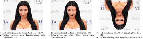
In the RS literature and common practice, where a large majority of ‘EO-IU ⊂ CV’ system solutions belongs to the most suboptimal 1D image analysis approach, specifically, pixel-based/2D spatial context-insensitive image analysis (see Figure 22(a) and Figure 24), a typical strategy to gain quality in EO image interpretation is to augment the (2D) raster data dimensionality with one additional data dimension, specifically, time, which explains the recent hype on EO (raster-based) data cubes (Open Data Cube, 2020; Baumann, 2017; CEOS – Committee on Earth Observation Satellites, 2020; Giuliani et al., 2017, 2020; Lewis et al., 2017; Strobl et al., 2017) (refer to Section 2). In practice, to recover from typically “low” OP-Q²I values affecting 2D spatial context-insensitive/1D pixel-based image analysis algorithms, 2D spatial context-insensitive pixel-through-time analysis is proposed instead. In (Camara, 2017), the pragmatic question raised by Gilberto Camara is:

In EO large image database analysis, “space first, time later or time first, space later”? Gilberto Camara’s practical answer is: “time first, space later”.

Unfortunately, in the RS common practice dominated by 1D image analysis algorithms, a pragmatic ‘CV ⊃ EO-IU’ approach where “time (comes) first, space (comes) later” is typically implemented as a pixel-through-time analysis in an image time-series (Picoli et al., 2018). Synonym for 2D spatial context-insensitive 1D vector data sequence analysis of a 3D (2D space + 1D time) data cube, pixel-through-time analysis of an image time-series is conceptually equivalent to a

“time first, space never” approach to video (image time-series) analysis.

Presented as such it would sound very suboptimal indeed, quite unappealing to a community of video experts and practitioners. Nevertheless, to date, pixel-through-time analysis of an EO image time-series is a standard approach in the RS meta-science domain.

4.2. Bayesian inference constraints for better conditioning an inherently ill-posed ‘EO-IU ⊂ CV ⊂ AGI’ system solution

To overcome the data dimensionality reduction problem, from 2D gridded data (imagery) to 1D vector data sequence, affecting non-retinotopic 1D image analysis algorithms (see Figure 22 and Figure 25) largely adopted by the RS community in coping with the six Vs of EO large image databases, starting from 2D spatial context-insensitive/pixel-based analysis of EO big imagery and pixel-through-time analysis of EO big data cubes (whose minimum data dimensionality is 3D, with 2D for imagery + 1D for time, also refer to Figure 39 below in this text), this Subsection proposes an original set of ‘EO-IU ⊂ CV ⊂ AGI ⊂ Cognitive science’ system requirements/constraints, inspired by the Marr constraints presented in the CV literature (Marr, 1982; Quinlan, 2012) and engaged with each of the Marr five levels of system understanding (refer to Subsection 3.2). In agreement with a Bayesian/ driven-by-prior knowledge/ class-conditional approach to data analysis (Bowers & Davis, 2012; Ghahramani, 2011; Lähteenlahti, 2021; Quinlan, 2012; Sarkar, 2018) (refer to Subsection 3.5), alternative to unconditional/driven-without-prior-knowledge data analysis, prior knowledge-based constraints, whose a priori knowledge is available in addition to sensory data, are required by inherently ill-posed ‘EO-IU ⊂ CV ⊂ AGI ⊂ Cognitive science’ systems (see Figure 20) to become: (i) better posed for numerical solution (refer to references listed in Subsection 3.3.2), and (ii) capable of joint optimization of an mDMI set of OP-Q²Is to be community-agreed upon (refer to Subsection 3.1).

Since relationship ‘EO-IU ⊂ CV ⊂ AGI’ holds, i.e. ‘CV ⊃ EO-IU’ is a special case of (subset-of, with inheritance) AGI, then, in agreement with a stepwise approach, the following set of ‘CV ⊃ EO-IU’ system constraints is expected to be more severe (specialized, domain-specific) than the general-purpose set of constraints proposed for AGI solutions in Subsection 3.5.

1. Marr levels of system understanding 1-of-5 and 2-of-5 (refer to Subsection 3.2): Input data requirements specification and information/knowledge representation. When an EO imaging sensor is provided with a radiometric Cal subsystem onboard, such as in high-quality spaceborne and airborne EO platforms, typically excluding small satellite (< 500 kg) constellations provided with no Cal subsystem onboard (Baraldi, 2019b), each EO image is acquired together with its radiometric Cal metadata file. In agreement with Subsection 3.5, whenever a radiometric Cal metadata file is available, then radiometric Cal of EO imagery is considered mandatory to augment EO image standardization/ harmonization/ interoperability across time, geospace and imaging sensors, in compliance with an intuitive general-purpose GIGO principle (Baraldi, 2017; Geiger et al., 2021; Thompson, 2018) (refer to Section 2), easy to understand based on commonsense knowledge (refer to references listed in Section 2), with the intergovernmental GEO-CEOS QA4EO Cal requirements (refer to references listed in Section 2) and with the standard FAIR principles for scientific data (product and process) management (refer to references listed in Section 2 and see Table 1).

   As reported in Subsection 3.3.2, radiometrically calibrated EO imagery is provided with a physical meaning, a physical unit of measure and a physical range of change. It can be employed as input to: (i) physical model-based (top-down, deductive) inference systems, requiring as input numerical variables provided with a physical meaning. (ii) Statistical (data-driven, bottom-up, inductive) algorithms. Although they do not require as input numerical variables provided with a physical meaning, they typically benefit from radiometric Cal of input variables, which are better behaved. (iii) Hybrid (combined deductive and inductive) inference systems, whose deductive/ top-down/ physical model-based system components require as input numerical variables provided with a physical meaning.

   When EO optical imagery is radiometrically calibrated into TOARF values at EO Level 1, SURF 1-of-3 to SURF 3-of-3 values at EO Level 2/ARD or surface albedo values at EO Level 3 or beyond, whose physical range of change is [0.0, 1.0], then Equation (8)(8) $\begin{array}{rl}& \text{lsquo}\mathrm{D}\mathrm{N}\mathrm{s}\ge 0\mathrm{a}\mathrm{t}\mathrm{E}\mathrm{O}\mathrm{L}\mathrm{e}\mathrm{v}\mathrm{e}\mathrm{l}0\supseteq \mathrm{T}\mathrm{O}\mathrm{A}\mathrm{R}\mathrm{F}\in \left[0.0,1.0\right]\mathrm{a}\mathrm{t}\mathrm{E}\mathrm{O}\mathrm{L}\mathrm{e}\mathrm{v}\mathrm{e}\mathrm{l}1\supseteq \mathrm{S}\mathrm{U}\mathrm{R}\mathrm{F}\in \left[0.0,1.0\right]\\ & \mathrm{a}\mathrm{t}\mathrm{E}\mathrm{O}\mathrm{L}\mathrm{e}\mathrm{v}\mathrm{e}\mathrm{l}2/\left(\mathrm{c}\mathrm{u}\mathrm{r}\mathrm{r}\mathrm{e}\mathrm{n}\mathrm{t}\right)\mathrm{A}\mathrm{R}\mathrm{D}\supseteq \mathrm{S}\mathrm{u}\mathrm{r}\mathrm{f}\mathrm{a}\mathrm{c}\mathrm{e}\mathrm{a}\mathrm{l}\mathrm{b}\mathrm{e}\mathrm{d}\mathrm{o}\in \left[0.0,1.0\right]\mathrm{a}\mathrm{t},\mathrm{s}\mathrm{a}\mathrm{y},\mathrm{E}\mathrm{O}\mathrm{L}\mathrm{e}\mathrm{v}\mathrm{e}\mathrm{l}3/\mathrm{n}\mathrm{e}\mathrm{x}\mathrm{t}\\ & \mathrm{g}\mathrm{e}\mathrm{n}\mathrm{e}\mathrm{r}\mathrm{a}\mathrm{t}\mathrm{i}\mathrm{o}\mathrm{n}\mathrm{A}\mathrm{R}\mathrm{D}\text{rsquo}& (8)\end{array}$(8) to Equation (11)(11) $\text{lsquo}\mathrm{T}\mathrm{O}\mathrm{A}\mathrm{R}\mathrm{F}\approx \mathrm{S}\mathrm{U}\mathrm{R}\mathrm{F}\text{rsquo}$(11) hold (refer to Subsection 3.3.2). These calibrated numerical variables in range [0.0, 1.0] can be encoded as unsigned byte in range {0, 255}, featuring a negligible quantization error ≈ 0.2% and a 50% saving in memory occupation in comparison with a 16-bit unsigned short integer encoding, typically adopted by the RS community (refer to references listed in Subsection 3.3.2).

2. Marr level of system understanding 1-of-5 (refer to Subsection 3.2): Outcome and process requirements specification. To be considered in operational mode (refer to Section 2), a ‘CV ⊃ EO-IU’ system is required to score “high” in an mDMI set of OP-Q²Is, such as that proposed in Subsection 3.1, to be community-agreed upon in advance, in agreement with the intergovernmental GEO-CEOS QA4EO Val guidelines (GEO-CEOS – Group on Earth Observations and Committee on Earth Observation Satellites, 2010). In an mDMI set of OP-Q²Is, multi-objective optimization pursues low bias (low error rate) in combination with (jointly with) low variance (low dependence on input data)/ high robustness to changes in input data/ high transferability/ high interoperability (see Figure 13), in agreement with the AGI outcome and process requirements specification proposed in Subsection 3.5, whereas ‘ML ⊃ DL ⊃ DCNN’ applications in the CV and RS meta-sciences typically feature low bias, but high variance (refer to Subsection 3.1), together with low interpretability, see Figure 14.

   Figure 26. Adapted from (DiCarlo, 2017). As instance of the science of Natural Intelligence, reverse engineering primate visual perception adopts a stepwise approach (Baraldi, 2017; Bharath & Petrou, 2008; DiCarlo, 2017), in agreement with the seminal work by Marr (Marr, 1982).

   

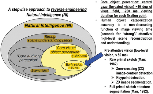
3. Marr levels of system understanding 1-of-5 to 5-of-5 (refer to Subsection 3.2): Outcome and process requirements specification, information/knowledge representation, system design (architecture), algorithm and implementation. Working hypothesis ‘Human vision → CV ⊃ EO-IU’ = Equation (4)(4) $\begin{array}{rl}& \text{lsquo}(Inductive/bottom\text{-}up/statisticalmodel\text{-}based)DL\text{-}from\text{-}data\subset \\ & (Inductive/bottom\text{-}up/statisticalmodel\text{-}based)ML\text{-}from\text{-}data\\ & \to AGI\supset CV\leftarrow Humanvision\text{rsquo}\end{array}$(4) (see Figure 11) means that human vision is adopted as lower bound of CV, i.e. to become better posed for numerical solution (refer to references listed in Subsection 3.3.2), an inherently ill-posed ‘CV ⊃ EO-IU’ system is required to include as part-of (without inheritance) a computational model of human vision, consistent with human vision perceptual phenomena (Baraldi, 2017; Baraldi et al., 2018a, 2018b; Baraldi & Tiede, 2018a, 2018b; Iqbal & Aggarwal, 2001).

   A straightforward approach to computational modelling human vision is reverse engineering primate visual perception (Baraldi, 2017; Baraldi et al., 2018a, 2018b; Baraldi & Tiede, 2018a, 2018b; Bharath & Petrou, 2008; DiCarlo, 2017; Hassabis et al., 2017; Iqbal & Aggarwal, 2001; Rappe, 2018; Slotnick et al., 2005; Vecera & Farah, 1997), see Figure 26. In the words of Qasim Iqbal and Jagdishkumar Aggarwal “biological vision is currently the only measure of the incompleteness of the current stage of computer vision, and illustrates that the problem is still open to solution” (Iqbal & Aggarwal, 2001).

   1. A first constraint stemming from reverse engineering primate visual perception (see Figure 26) requires an inherently ill-posed ‘CV ⊃ EO-IU’ system to embed by design a hybrid (combined deductive and inductive) inference approach, in agreement with Subsection 3.5.

      In general, biological cognitive systems, suitable for exploiting the four inference mechanisms investigated by formal logic (refer to Subsection 3.3.4), are hybrid inference systems, where a priori genotype provides initial conditions to learning-from-examples phenotype (Baraldi, 2017; Parisi, 1991; Zador, 2019). According to genetic epistemology, in biological cognitive systems, “there is never an absolute beginning” (Piaget, 1970) (refer to Subsection 3.3.4).

      A special case of biological cognitive (sub)system is the primate visual (sub)system (refer to references listed in Section 2). It accomplishes an early vision/low-level vision first phase, which is pre-attentional (unconscious, non-attentive), parallel and fast (< 50 ms), followed by an attentional vision/high-level vision second phase, which is conscious, slow (in terms of secs) and sequential in nature (DiCarlo, 2017; Kosslyn, 1994; Mason & Kandel, 1991), see Figure 26. In the Marr terminology, within early vision, a pre-attentive raw primal sketch, synonym for image segmentation/partitioning, is preliminary to a pre-attentional full primal sketch (Marr, 1982), synonym for texture segmentation (perceptual grouping of texture elements, texels, or tokens) (Baraldi, 2017; Cherry, 2019; Geirhos et al., 2018; Green, 1997; Jain & Healey, 1998; Julesz, 1986; Julesz et al., 1973; Koffka, 1935; Tuceryan, 1992; Victor, 1994; Yellott, 1993). Noteworthy, to date, no texture segmentation algorithm in operational mode exists (in compliance with the definition proposed in Subsection 3.1).

      In humans, at the first phase of early vision (see Figure 26), image segmentation/partitioning (raw primal sketch) (Baraldi, 2017; Marr, 1982) is an example of inherently ill-posed hybrid (combined deductive and inductive) inference subsystem. In the words of Shaun Vecera and Martha Farah “we have demonstrated that [low-level, pre-attentional] image segmentation [as the dual problem of image-contour detection] is inherently ill-posed [in the Hadamard sense]. It can be influenced by the familiarity of the shape being segmented … these results are consistent with the hypothesis that image segmentation is an interactive [hybrid inference] process … in which top-down knowledge partly guides lower level processing” (Vecera & Farah, 1997) (refer to Subsection 4.1).

      Noteworthy, a hybrid ‘CV ⊃ EO-IU’ inference approach is alternative to increasingly popular inductive/bottom-up ‘DCNN ⊂ DL ⊂ ML’ algorithms (Cimpoi et al., 2014; Krizhevsky et al., 2012), learned from data end-to-end starting from scratch (tabula rasa, actually, starting from a set of model hyperparameters to be user-defined based on heuristics, equivalent to prior knowledge to be encoded by design, refer to Subsection 3.1).

   2. As discussed in Subsection 4.1, a second constraint stemming from reverse engineering primate visual perception (see Figure 26) requires an inherently ill-posed ‘CV ⊃ EO-IU’ system to embed by design a retinotopic/2D spatial topology-preserving image mapping approach (Baraldi, 2017; Baraldi & Alpaydin, 2002a, 2002b; Fritzke, 1997; Martinetz et al., 1994; Öğmen & Herzog, 2010; Tsotsos, 1990), synonym for 2D analysis of (2D) imagery by means of a 2D grid (array) of 2D spatial filters, see Figures 23 and 24.

      At the Marr levels of system understanding 3-of-5 (system design), 4-of-5 (algorithm) and 5-of-5 (implementation), spatial topology-preserving 2D analysis of (2D) imagery can be pursued by a multi-scale hierarchy of 2D arrays (grids, networks) of 2D spatial filters (see Figure 23), either isotropic (Burt & Adelson, 1983; Marr, 1982) or oriented (Baraldi, 2017; Jain & Healey, 1998), even- or odd-symmetric (Baraldi, 2017; Burt & Adelson, 1983; Canny, 1986; Jain & Healey, 1998; Mallat, 2009; Marr, 1982), either low-pass (e.g. Gaussian), band-pass or high-pass (Baraldi, 2017; Jain & Healey, 1998; Mallat, 2009), etc. A multi-scale hierarchy of 2D spatial filters can be implemented either top-down or bottom-up.

      • Top-down/ physical model-based /deductive /“handcrafted” 2D wavelet-based filter bank, whose 2D spatial filters are typically provided with a high degree of biological plausibility (refer to references listed in Subsection 4.1), including retinotopic/2D spatial topology-preserving feature mapping capabilities, see Figure 23. Or

      • Bottom-up/inductive DCNN, typically learned from data end-to-end (Cimpoi et al., 2014; Krizhevsky et al., 2012). Unfortunately, due to bad practices in multi-scale spatial filter implementation (Geirhos et al., 2018; Zhang, 2019), modern inductive learning-from-data DCNNs typically neglect the spatial ordering of object parts, i.e. they are insensitive to the shuffling of image parts (Brendel, 2019; Brendel & Bethge, 2019), see Figure 25. In practice, large portions of modern DCNNs adopt a decision strategy very similar to that of traditional 1D image analysis approaches (see Figure 22), such as bag-of-local-features models (Brendel, 2019; Brendel & Bethge, 2019), which are insensitive to permutations in the 1D sequence of input data (Bourdakos, 2017) (refer to Subsection 4.1).

      In summary, synonym for retinotopic/2D spatial topology-preserving image analysis, 2D image analysis in operational mode is alternative to, first, 1D image analysis approaches, synonym for non-retinotopic 1D analysis of (2D) imagery (see Figure 22), currently dominating the RS literature and the RS common practice. Second, (retinotopic) 2D image analysis is alternative to several inductive ‘DCNN ⊂ DL ⊂ ML’ system implementations, whose multi-scale 2D arrays of 2D spatial filters are theoretically consistent with retinotopic/2D spatial topology-preserving image decomposition (Burt & Adelson, 1983), image reconstruction (Burt & Adelson, 1983) and image analysis/understanding (see Figure 23), but whose non-retinotopic image mapping behavior is similar to that of traditional 1D image analysis approaches (Bourdakos, 2017), such as bag-of-local-features models (Brendel, 2019; Brendel & Bethge, 2019), see Figure 25.

   3. A third family of constraints stemming from reverse engineering primate visual perception (see Figure 26) focuses on so-called visual illusion phenomena (illusory contours) (Baraldi, 2017; Mély et al., 2018; Perez, 2018; Pessoa, 1996; Rappe, 2018). About visual illusions, a quote of interest by Thomas Serre is (Mély et al., 2018; Rappe, 2018): “there is growing consensus that optical illusions are not a bug, but a feature. I think they are a feature. They may represent edge cases for our visual system, but our vision is so powerful in day-to-day life and in recognizing objects.” According to Luiz Pessoa (Pessoa, 1996), “if we require that a CV system should be able to predict perceptual effects, such as the well-known Mach bands illusion where bright and dark bands are seen at ramp edges, then the number of published vision models becomes surprisingly small”, see Figure 27. In more detail (Baraldi, 2017; Baraldi & Tiede, 2018a, 2018b), the Mach bands illusion proves that, if image-segments/image-contours detected by a ‘CV ⊃ EO-IU’ system are required to be consistent with human visual perception, including ramp-edge detection independent of the ramp slope, then popular local image statistics in ‘CV ⊃ EO-IU’ algorithms, namely, local image variance, contrast and 1st-order derivative (gradient), sensitive to a ramp slope, are not suitable visual features, see Figure 27.

      This straightforward (obvious), but not trivial observation (true-fact) is at odd with a large portion of the existing CV and RS literature, where many ‘CV ⊃ EO-IU’ algorithms, specifically, semi-automatic image segmentation (partitioning) algorithms, based on either connected-region growing criteria (Baatz & Schäpe, 2000; Camara et al., 1996; Espindola et al., 2006) or, vice versa, non-connected image-contour detection by means of 2D spatial filters (Heitger et al., 1992; Pessoa, 1996; Rodrigues & Du Buf, 2009), such as the popular Canny edge detector (Canny, 1986), typically employ as decision rule some empirical thresholding of local (e.g. region-based, local window-based, 2D spatial filter activation domain-specific, etc.) image statistics, such as local variance, local contrast or first-order gradient.

      The conclusion is that, to better condition an inherently ill-posed ‘CV ⊃ EO-IU’ system for numerical solution (Baraldi, 2017; Baraldi et al., 2018a, 2018b; Baraldi & Tiede, 2018a, 2018b; Bishop, 1995; Cherkassky & Mulier, 1998; Dubey et al., 2018), a prior knowledge-based constraint to be embedded by design in the ‘CV ⊃ EO-IU’ system, where a 2D array of 2D spatial filters is required for 2D image analysis (refer to this Subsection above), is compliance by design with the Mach bands visual illusion (Baraldi, 2017; Baraldi & Tiede, 2018a, 2018b; Pessoa, 1996), where bright and dark bands are automatically perceived at ramp edges, independent of the ramp slope, see Figure 27.

      Figure 27. Mach bands visual illusion (Pessoa, 1996). Below, in the image profile, in black: Ramp in (true, quantitative) luminance units across space. In red: Brightness (qualitative, perceived luminance) across space, where brightness is defined as a subjective aspect of vision, i.e. brightness is the perceived luminance of a surface (Boynton, 1990). Where a luminance (radiance, intensity) ramp meets a plateau, there are spikes of brightness, although there is no discontinuity in the luminance profile. Hence, human vision detects two boundaries, one at the beginning and one at the end of the ramp in luminance, independent of the ramp slope. Since there is no discontinuity in luminance where brightness is spiking, the Mach bands effect is called a visual ‘illusion’. In the words of Luiz Pessoa, ‘if we require that a brightness model should at least be able to predict Mach bands, the bright and dark bands which are seen at ramp edges, the number of published models is surprisingly small’ (Pessoa, 1996). The important lesson to be learned from the Mach bands illusion is that, in vision, local variance, contrast and 1st-order derivative (gradient) are statistical features (data-derived numerical variables) computed locally in the (2D) image-domain not suitable to detect image-objects (segments, closed contours) required to be perceptually ‘uniform’ (‘homogeneous’) in agreement with human vision (Baraldi, 2017; Baraldi et al., 2018a, 2018b; Baraldi & Tiede, 2018a, 2018b; Iqbal & Aggarwal, 2001). In other words, these popular local statistics, namely, local variance, contrast and 1st-order derivative (gradient), are not suitable visual features if detected image-segments and/or image-contours are required to be consistent with human visual perception, including ramp-edge detection. This straightforward (obvious), but not trivial observation is at odd with a large portion of the existing computer vision (CV) and remote sensing (RS) literature, where many CV algorithms for semi-automatic image segmentation (Baatz & Schäpe, 2000; Camara et al., 1996; Espindola et al., 2006) or (vice versa) semi-automatic image-contour detection (Heitger et al., 1992), such as the popular Canny edge detector (Canny, 1986), are based on empirical thresholding the local variance, contrast or first-order gradient based on data-dependent heuristic criteria.

      

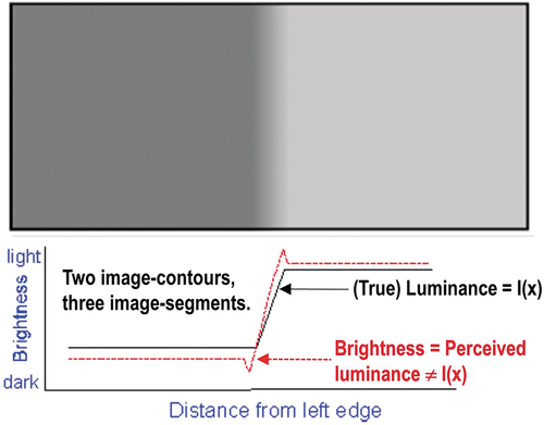
   4. As discussed in Subsection 4.1, in reverse engineering primate visual perception (see Figure 26), a fourth perceptual constraint is that spatial information, mapped from the 4D scene-domain onto the (2D) image-plane (see Figure 20), typically dominates colorimetric information, see Figure 21. To prove that a ‘CV ⊃ EO-IU’ system fully exploits primary/dominant 2D spatial topological and 2D spatial non-topological information components in addition to secondary/subordinate colorimetric information in the (2D) image-plane, an original necessary-and-sufficient condition for a CV system to accomplish robustness to changes in input data and scalability to changes in sensor specifications (refer to Subsection 3.1) is formulated as follows (Baraldi, 2017).

      If a chromatic ‘CV ⊃ EO-IU’ system does not down-scale seamlessly to achromatic/panchromatic (PAN) image analysis, then it tends to ignore the paramount (primary, dominant) 2D spatial topological and non-topological information components in the (2D) image-plane (refer to Subsection 4.1) in favor of a subordinate (secondary) spatial context-insensitive color information, such as in traditional ‘EO-IU ⊂ CV’ systems where colorimetric information, available at the sensor resolution as a pixel-based MS or HS or SS signature (see Figure 7), either single-date or multi-temporal, is investigated exclusively, by means of a 2D spatial context-insensitive/1D pixel-based image analysis approach, see Figure 22(a).

      In other words, a necessary-and-sufficient condition for a ‘CV ⊃ EO-IU’ system to fully exploit, in the (2D) image-plane, primary/dominant 2D spatial topological and 2D spatial non-topological information components in combination with (jointly with, according to a convergence-of-evidence approach) secondary/subordinate colorimetric information, mapped (projected) from a 4D geospace-time scene-domain onto a (2D) image-plane by an imaging sensor, is to perform nearly as well in the joint optimization of a community-agreed mDMI set of OP-Q²Is (such as that proposed in Subsection 3.1) when input with either achromatic/PAN imagery or chromatic/color imagery, where color imagery ranges from MS to SS and HS imagery (refer to Section 2).

   As proof of suitability and feasibility of constraints (i) to (iv) listed above, stemming from reverse engineering primate visual perception (see Figure 26), let us consider a realization of a hybrid two-stage ‘CV ⊃ EO-IU’ software system prototype, suitable for early (pre-attentive) vision tasks, where these four constraints, inferred from a priori knowledge of primate visual perception in agreement with Equation (4)(4) $\begin{array}{rl}& \text{lsquo}(Inductive/bottom\text{-}up/statisticalmodel\text{-}based)DL\text{-}from\text{-}data\subset \\ & (Inductive/bottom\text{-}up/statisticalmodel\text{-}based)ML\text{-}from\text{-}data\\ & \to AGI\supset CV\leftarrow Humanvision\text{rsquo}\end{array}$(4) = ‘Human vision → CV ⊃ EO-IU’ (see Figure 11), are encoded by design (Baraldi, 2017; Baraldi & Tiede, 2018a, 2018b).

   Figure 28. To comply with working hypothesis ‘Human vision → CV ⊃ EO-IU’ = Equation (4)(4) $\begin{array}{rl}& \text{lsquo}(Inductive/bottom\text{-}up/statisticalmodel\text{-}based)DL\text{-}from\text{-}data\subset \\ & (Inductive/bottom\text{-}up/statisticalmodel\text{-}based)ML\text{-}from\text{-}data\\ & \to AGI\supset CV\leftarrow Humanvision\text{rsquo}\end{array}$(4) (see Figure 11), a low-level ‘CV ⊃ EO-IU’ subsystem is implemented as a top-down/ deductive/ physical model-based (“handcrafted”) 2 grid (array) of wavelet-based multi-scale multi-orientation low-pass 2D Gaussian filters and band-pass trimodal even-symmetric 2D spatial filters (Baraldi, 2017). It is equivalent to a prior knowledge-based (physical model-based) deep convolutional neural network (DCNN), alternative to popular inductive DCNNs learned-from-data end-to-end (Cimpoi et al., 2014; Krizhevsky et al., 2012). Capable of automatic zero-crossing image-contour detection and image segmentation/partitioning, it complies with human visual perception (Baraldi, 2017; Baraldi et al., 2018a, 2018b; Baraldi & Tiede, 2018a, 2018b; Iqbal & Aggarwal, 2001), with regard to: (1) the Mach bands visual illusion (Pessoa, 1996) and (2) the perceptual true-fact that human panchromatic and chromatic vision mechanisms are nearly as effective in scene-from-image reconstruction and understanding. It is tested on complex spaceborne/airborne EO optical images in agreement with a stepwise approach, consistent with the property of systematicity of natural language/thought (Fodor, 1998; Peirce, 1994; Rescorla, 2019; Saba, 2020a) (refer to Subsection 3.4), to be regarded as commonsense knowledge, agreed upon by the entire human community (refer to Section 2). Testing images start from “simple” synthetic imagery of “known”, but challenging complexity in 2D spatial and colorimetric information components. If first-level testing with synthetic imagery is successful, next, natural panchromatic and RGB images, intuitive to cope with, are adopted for second-level testing purposes. Finally, complex spaceborne/airborne EO optical imagery, depicting manmade objects of known shape and size together with textured areas, are employed for third-level testing. (a) SUSAN synthetic panchromatic image, byte encoded in range {0, 255}, image size (rows × columns × bands) = 370 × 370 × 1. No histogram stretching applied for visualization purposes. Step edges and ramp edges at known locations (the latter forming the two inner rectangles visible at the bottom right corner) form angles from acute to obtuse. According to human vision, 31 image-segments can be detected as reference “ground-truth”. (b) Sum (synthesis) of the wavelet-based near-orthogonal multi-scale multi-orientation image decomposition. Filter value sum in range from −255.0 to +255.0. (c) Automated (requiring no human–machine interaction) image segmentation into zero-crossing segments generated from zero-crossing pixels detected by the multi-scale multi-orientation trimodal even-symmetric 2D spatial filter bank, different from Marr’s single-scale isotropic zero-crossing pixel detection (Marr, 1982). Exactly 31 image-segments are detected with 100% contour accuracy. Segment contours depicted with 8-adjacency cross-aura values in range {0, 8}, see Figure 31. (d) Image-object mean view = object-wise constant input image reconstruction. No histogram stretching applied for visualization purposes. (e) Object-wise constant input image reconstruction compared with the input image, per-pixel root mean square error (RMSE) in range [0.0, 255.0], equivalent to a vector discretization/quantization (VQ) quality assessment in image decomposition (analysis, encoding) and reconstruction (synthesis, decoding) (Baraldi, 2017, 2019a; Baraldi et al., 2010a, 2010b, 2018a, 2018b, 2006; Baraldi & Tiede, 2018a, 2018b). (f) Natural panchromatic image of an actress wearing a Venetian carnival mask, image size (rows × columns × bands) = 438 × 310 × 1. No histogram stretching applied for visualization purposes. (g) Same as (b). (h) Same as (c), there is no CV system’s free- parameter to be user-defined. (i) Same as (d). (l) Same as (e). (m) Natural RGB-color image of an actress wearing a Venetian carnival mask, image size (rows × columns × bands) = 438 × 310 × 3. No histogram stretching applied for visualization purposes. (n) Same as (b). (o) Same as (c), there is no CV system’s free- parameter to be user-defined. (p) Same as (d). (q) Same as (e). (r) Zoom-in of a Sentinel-2A MSI Level-1 C image of the Earth surface south of the city of Salzburg, Austria. Acquired on 2015–09-11. Spatial resolution: 10 m. Radiometrically calibrated into top-of-atmosphere reflectance (TOARF) values in range [0.0, 1.0], byte-coded into range {0, 255}, it is depicted as a false color RGB image, where: R = Middle-InfraRed (MIR) = Band 11, G = Near IR (NIR) = Band 8, B = Blue = Band 2. Standard ENVI histogram stretching applied for visualization purposes. Image size (rows × columns × bands) = 545 × 660 × 3. (s) Same as (b). (t) Same as (c), there is no CV system’s free-parameter to be user-defined. (u) Same as (d), but now a standard ENVI histogram stretching is applied for visualization purposes. (v) Same as (e).

   

   Figure 28. Continued.

   

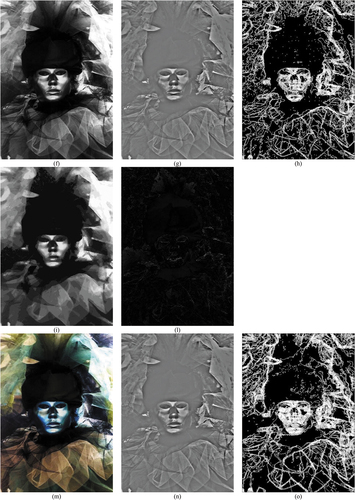
   Figure 28. Continued.

   

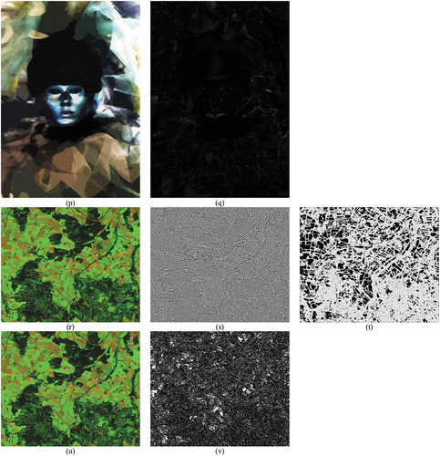
   The original hybrid (combined physical and statistical model-based) automatic (requiring no human-machine interaction to run) two-stage ‘CV ⊃ EO-IU’ software system prototype, whose PAN and MS image-derived output products are shown in Figure 28, is described below.

   • The first stage of the two-stage ‘CV ⊃ EO-IU’ software system prototype consists of a biologically plausible top-down/ deductive/ physical model-based (“hand-crafted”) 2D array of wavelet-based multi-scale and multi-orientation low-pass 2D Gaussian filters and band-pass trimodal even-symmetric 2D spatial filters (Baraldi, 2017; Burt & Adelson, 1983; DiCarlo, 2017; Jain & Healey, 1998; Mallat, 2009; Marr, 1982; Sonka et al., 1994), suitable for: (i) lossless (as alternative to lossy) multi-scale PAN or MS image analysis/decomposition and synthesis/reconstruction (Burt & Adelson, 1983) and (ii) zero-crossing image-contour detection (Baraldi, 2017; Baraldi & Tiede, 2018a, 2018b; Marr, 1982), in both PAN and MS imagery, with image-contours due to three edge primitives, either step edge, line edge or ramp edge, plus their possible combinations, where ramp-edge detection complies with the Mach bands visual illusion (Baraldi, 2017), see Figure 27. Oriented trimodal even-symmetric 2D spatial wavelet filters provide local estimates of the image concavity, equivalent to oriented 2^nd-order derivatives of the 2D gridded data (Baraldi, 2017).

     Noteworthy, in agreement with the Mach bands visual illusion (see Figure 27), local image concavity/2^nd-order derivative is alternative to local image statistics typically adopted in low-level (pre-attentional) image-contour detection algorithms (Canny, 1986; Sonka et al., 1994) or region-growing algorithms for low-level image segmentation/partitioning (Baatz & Schäpe, 2000; Camara et al., 1996; Espindola et al., 2006; Sonka et al., 1994), such as local image gradient/1st-order derivative, local variance and local contrast.

     The proposed physical model-based (“hand-crafted”) multi-scale multi-orientation 2D array of 2D spatial filters is a top-down/deductive DCNN instantiation, alternative to popular bottom-up/inductive DCNNs featuring millions of free-parameters to be learned-from-data end-to-end (Cimpoi et al., 2014; Krizhevsky et al., 2012; Marcus, 2018, 2020). The proposed first-stage deductive DCNN is, first, automatic, i.e. it features no system hyperparameters to be user-defined based on heuristics (refer to Subsection 3.1); hence, it requires no human-machine interaction to run. Second, it features no model’s free-parameter to be learned from data (refer to Subsection 3.1), i.e. it is static (non-adaptive to data). Actually, it needs no adaptivity to data because it is capable of lossless multi-scale image decomposition and reconstruction, whatever the input image is, either achromatic/PAN or chromatic/MS.

   • The first-stage deductive/physical model-based 2D spatial filter bank for zero-crossing image-contour detection is followed by an inductive (bottom-up, data-driven) image mapping second stage, suitable for automatic multi-level (categorical) image partitioning into so-called zero-crossing segments (Baraldi, 2017; Marr, 1982). The three image-levels/ layers/ strata to be deterministically partitioned into segments consist of zero concavity, negative concavity and positive concavity values detected by the first stage (Baraldi, 2017; Marr, 1982). This second-stage multi-level image segmentation task is deterministic (well-posed), i.e. it admits a unique solution (Hadamard, 1902). It is solved by a well-known two-pass connected-component multi-level image labeling algorithm, whose computational complexity is linear with image size (Dillencourt et al., 1992; Sonka et al., 1994), refer to Figure 31(a) below in this Subsection.

     Noteworthy, image segmentation/partitioning in the 2D spatial domain of a 2D gridded categorical variable (multi-level image) is deterministic/well-posed in linear complexity with image size (see Figure 31(a) below in this Subsection), unlike traditional algorithms for low-level image segmentation in the 2D spatial domain of a 2D gridded numerical variable (image) (Baatz & Schäpe, 2000; Camara et al., 1996; Espindola et al., 2006), which are inherently ill-posed (Vecera & Farah, 1997) (refer to Section 4.1) and require prior knowledge in addition to 2D gridded data (imagery) to become better posed for numerical solution (refer to references listed in Subsection 3.3.2).

     Figure 28 shows low-level vision results collected by the aforementioned hybrid two-stage ‘CV ⊃ EO-IU’ software system prototype when it is input with either achromatic/PAN or chromatic/MS testing images of increasing levels of complexity, in agreement with a stepwise approach, consistent with the property of systematicity of natural language/thought (Fodor, 1998; Peirce, 1994; Rescorla, 2019; Saba, 2020a) (refer to Subsection 3.4), to be regarded as commonsense knowledge, agreed upon by the entire human community (refer to Section 2). In more detail, the set of testing images of increasing complexity in 2D spatial information and colorimetric information components comprises, first, a synthetic PAN image of known geometric and radiometric quality, consisting of thirty-one image-regions (as known “ground/reference-truth”) provided with step edges and ramp edges (see Figure 27). Second, a natural PAN image intuitive to understand by a human photointepreter (i.e. an image whose interpretation/meaning/semantics and “ground-truth” are known/agreed upon, based on commonsense knowledge). Third, the same natural image in RGB true-colors. Fourth, an EO spaceborne MS image of the Earth surface characterized by the presence of surface-objects featuring a large variety of visual (appearance) properties, such as agricultural fields, typically provided with straight boundaries (refer to this Subsection below), which is a geometric property typical of human artefacts, in combination with within-field “low” texture, forest areas typically characterized by “high” texture of the forest cover, etc. (refer to Subsection 4.1).

     Worth noting, the property of systematicity, typical of natural language/thought (refer to references listed in Subsection 3.4), is traditionally ignored in the testing and (third-party independent) validation of ‘DL ⊂ ML’ algorithms, whose training and testing accuracy quality indexes collected upon big data are subject to the central limit theorem (Kreyszig, 1979; Sheskin, 2000; Tabachnick & Fidell, 2014), where non-stationarities in quality index distributions are lost (wiped out) (refer to Section 2).

4. Marr levels of system understanding 2-of-5 to 4-of-5 (refer to Subsection 3.2): Information/knowledge representation, system design and algorithm. To make an inherently ill-posed ‘CV ⊃ EO-IU’ system (see Figure 20) better posed for numerical solution (refer to references listed in Subsection 3.3.2), additional constraints, based on a priori knowledge, which is available in addition to sensory data, are applied to primary/dominant 2D spatial information and secondary/subordinate colorimetric information components in the (2D) image-plane (refer to Subsection 4.1).

   It is well known that, preliminary to feature (pattern) recognition (analysis, classification, understanding), feature engineering, either feature selection or feature extraction (Bishop, 1995; Cherkassky & Mulier, 1998), is of fundamental importance, e.g. to cope with the curse of data dimensionality, well-known in the ML-from-finite-data paradigm (Bishop, 1995; Cherkassky & Mulier, 1998). For example, in the meta-science domain of ‘ML ⊃ DL ⊃ DCNN’ applications, it is acknowledged that “proper feature engineering will have a much larger impact on model performance than even the most extensive hyperparameter tuning. It is the law of diminishing returns applied to machine learning: feature engineering gets you most of the way there, and hyperparameter tuning generally only provides a small benefit” (Koehrsen, 2018), see Figure 13.

   In feature engineering for CV applications, useful/informative 2D spatial feature and colorimetric feature extraction/representation is performed in the (2D) image-domain (see Figure 20) at the Marr second level of system abstraction, specifically, information/knowledge representation (refer to Subsection 3.2), by a low-level (pre-attentional, fast and parallel) CV first stage as necessary-but-not-sufficient pre-condition to a high-level (attentional, slow and sequential) CV second stage (Baraldi, 2017) (see Figure 26), where the latter adopts a convergence of primary spatial evidence with secondary color evidence approach (refer to Equation (12)(12) $\begin{array}{rl}& \mathrm{M}\mathrm{I}\mathrm{N}\left\{\begin{array}{c}\mathrm{m}\left(\mathrm{C}\mathrm{o}\mathrm{l}\mathrm{o}\mathrm{r}\mathrm{V}\mathrm{a}\mathrm{l}\mathrm{u}\mathrm{e}\left(\mathrm{x}\right)|\mathrm{c}\right),\mathrm{m}\left(\mathrm{S}\mathrm{i}\mathrm{z}\mathrm{e}\mathrm{V}\mathrm{a}\mathrm{l}\mathrm{u}\mathrm{e}\left(\mathrm{x}\right)|\mathrm{c}\right),\\ \mathrm{m}\left(2\mathrm{D}\mathrm{s}\mathrm{h}\mathrm{a}\mathrm{p}\mathrm{e}\mathrm{V}\mathrm{a}\mathrm{l}\mathrm{u}\mathrm{e}\left(\mathrm{x}\right)|\mathrm{c}\right),\mathrm{m}\left(\mathrm{T}\mathrm{e}\mathrm{x}\mathrm{t}\mathrm{u}\mathrm{r}\mathrm{e}\mathrm{V}\mathrm{a}\mathrm{l}\mathrm{u}\mathrm{e}\left(\mathrm{x}\right)|\mathrm{c}\right),\\ \mathrm{m}\left(2\mathrm{D}\mathrm{s}\mathrm{p}\mathrm{a}\mathrm{t}\mathrm{i}\mathrm{a}\mathrm{l}\mathrm{R}\mathrm{e}\mathrm{l}\mathrm{a}\mathrm{t}\mathrm{i}\mathrm{o}\mathrm{n}\mathrm{s}\mathrm{h}\mathrm{i}\mathrm{p}\mathrm{s}\left(\mathrm{x},2\mathrm{D}\mathrm{n}\mathrm{e}\mathrm{i}\mathrm{g}\mathrm{h}\left(\mathrm{x}\right)\right)|\mathrm{c}\right)\end{array}\right\}\\ & =\mathrm{M}\mathrm{I}\mathrm{N}\left\{\begin{array}{c}\sum _{\mathrm{C}\mathrm{o}\mathrm{l}\mathrm{o}\mathrm{r}\mathrm{N}\mathrm{a}\mathrm{m}{\mathrm{e}}_{\mathrm{j}},\mathrm{e}.\mathrm{g}.,\mathrm{r}\mathrm{e}\mathrm{d},\mathrm{g}\mathrm{r}\mathrm{e}\mathrm{e}\mathrm{n},\mathrm{b}\mathrm{l}\mathrm{u}\mathrm{e},\mathrm{e}\mathrm{t}\mathrm{c}.,\mathrm{w}\mathrm{i}\mathrm{t}\mathrm{h}\mathrm{j}=1}^{\mathrm{C}\mathrm{o}\mathrm{l}\mathrm{o}\mathrm{r}\mathrm{V}\mathrm{o}\mathrm{c}\mathrm{a}\mathrm{b}\mathrm{u}\mathrm{l}\mathrm{a}\mathrm{r}\mathrm{y}\mathrm{C}\mathrm{a}\mathrm{r}\mathrm{d}\mathrm{i}\mathrm{n}\mathrm{a}\mathrm{l}\mathrm{i}\mathrm{t}\mathrm{y}}\\ \mathrm{m}\left(\mathrm{C}\mathrm{o}\mathrm{l}\mathrm{o}\mathrm{r}\mathrm{V}\mathrm{a}\mathrm{l}\mathrm{u}\mathrm{e}\left(\mathrm{x}\right)|\mathrm{C}\mathrm{o}\mathrm{l}\mathrm{o}\mathrm{r}\mathrm{N}\mathrm{a}\mathrm{m}{\mathrm{e}}_{\mathrm{j}}\right)\mathrm{m}\left(\mathrm{C}\mathrm{o}\mathrm{l}\mathrm{o}\mathrm{r}\mathrm{N}\mathrm{a}\mathrm{m}{\mathrm{e}}_{\mathrm{j}}|\mathrm{c}\right),\\ \mathrm{m}\left(\mathrm{S}\mathrm{i}\mathrm{z}\mathrm{e}\mathrm{V}\mathrm{a}\mathrm{l}\mathrm{u}\mathrm{e}\left(\mathrm{x}\right)|\mathrm{c}\right),\mathrm{m}\left(2\mathrm{D}\mathrm{s}\mathrm{h}\mathrm{a}\mathrm{p}\mathrm{e}\mathrm{V}\mathrm{a}\mathrm{l}\mathrm{u}\mathrm{e}\left(\mathrm{x}\right)|\mathrm{c}\right),\\ \mathrm{m}\left(\mathrm{T}\mathrm{e}\mathrm{x}\mathrm{t}\mathrm{u}\mathrm{r}\mathrm{e}\mathrm{V}\mathrm{a}\mathrm{l}\mathrm{u}\mathrm{e}\left(\mathrm{x}\right)|\mathrm{c}\right),\\ \mathrm{m}\left(2\mathrm{D}\mathrm{s}\mathrm{p}\mathrm{a}\mathrm{t}\mathrm{i}\mathrm{a}\mathrm{l}\mathrm{R}\mathrm{e}\mathrm{l}\mathrm{a}\mathrm{t}\mathrm{i}\mathrm{o}\mathrm{n}\mathrm{s}\mathrm{h}\mathrm{i}\mathrm{p}\mathrm{s}\left(\mathrm{x},2\mathrm{D}\mathrm{n}\mathrm{e}\mathrm{i}\mathrm{g}\mathrm{h}\left(\mathrm{x}\right)\right)|\mathrm{c}\right)\end{array}\right\}\\ & =\mathrm{M}\mathrm{I}\mathrm{N}\{\mathrm{m}\left(\mathrm{C}\mathrm{o}\mathrm{l}\mathrm{o}\mathrm{r}\mathrm{N}\mathrm{a}\mathrm{m}{\mathrm{e}}^{\ast }|\mathrm{c}\right)\in \left\{0,1\right\},\mathrm{m}\left(\mathrm{S}\mathrm{i}\mathrm{z}\mathrm{e}\mathrm{V}\mathrm{a}\mathrm{l}\mathrm{u}\mathrm{e}\left(\mathrm{x}\right)|\mathrm{c}\right)\in \left[0.0,1.0\right],\\ & \mathrm{m}\left(2\mathrm{D}\mathrm{s}\mathrm{h}\mathrm{a}\mathrm{p}\mathrm{e}\mathrm{V}\mathrm{a}\mathrm{l}\mathrm{u}\mathrm{e}\left(\mathrm{x}\right)|\mathrm{c}\right)\in \left[0.0,1.0\right],\mathrm{m}\left(\mathrm{T}\mathrm{e}\mathrm{x}\mathrm{t}\mathrm{u}\mathrm{r}\mathrm{e}\mathrm{V}\mathrm{a}\mathrm{l}\mathrm{u}\mathrm{e}\left(\mathrm{x}\right)|\mathrm{c}\right)\in \left[0.0,1.0\right],\\ & \mathrm{m}\left(2\mathrm{D}\mathrm{s}\mathrm{p}\mathrm{a}\mathrm{t}\mathrm{i}\mathrm{a}\mathrm{l}\mathrm{R}\mathrm{e}\mathrm{l}\mathrm{a}\mathrm{t}\mathrm{i}\mathrm{o}\mathrm{n}\mathrm{s}\mathrm{h}\mathrm{i}\mathrm{p}\mathrm{s}\left(\mathrm{x},2\mathrm{D}\mathrm{n}\mathrm{e}\mathrm{i}\mathrm{g}\mathrm{h}\left(\mathrm{x}\right)\right)|\mathrm{c}\right)\in \left[0.0,1.0\right]\}\end{array}$(12) below in this Subsection), in agreement with primate visual perception (Mason & Kandel, 1991; Matsuyama & Hwang, 1990), see Figure 21.

   In more detail, low-level primary/dominant 2D spatial feature extraction and secondary/subordinate color feature extraction to be accomplished by a pre-attentional CV first stage are described below.

   1. Primary/dominant 2D spatial information representation in the (2D) image-plane. In agreement with Subsection 4.1, primary/dominant 2D spatial topological and spatial non-topological information components in the (2D) image-domain are partitioned into five statistically independent (refer to Section 2) feature categories.

      • Detected as raw primal sketch (Marr, 1982) in a pre-attentive CV first phase (Baraldi, 2017; Mason & Kandel, 1991), an image segmentation/partition consists of connected image-objects. An image-object is a planar spatial unit (Wikipedia, 2014a, 2014b), also known as segment (Baraldi, 2017; Marr, 1982), region (Perona & Malik, 1990), connected-component (Dillencourt et al., 1992) or token (Cherry, 2019; Green, 1997; Koffka, 1935; Marr, 1982; Tuceryan, 1992). The type of an image-object is either 0D (pixel), 1D (line) or 2D (polygon), in agreement with the OGC nomenclature (OGC – Open Geospatial Consortium Inc, 2015). The shape of an image-object is required to be parameterized according to an mDMI set of scale-invariant planar shape (geometric) indexes, such as that proposed in (Baraldi, 2017; Baraldi & Soares, 2017), where planar shape indexes are instances of scale-invariant 2D spatial non-topological features/attributes of an image-object.

        For example, in (Baraldi, 2017; Baraldi & Soares, 2017), the proposed mDMI set of scale-invariant planar shape indexes includes: (i) scale-invariant roundness (compactness and no holiness) in range [0.0, 1.0], which requires estimation of a 4-adjacency shape-contour length (refer to Figure 31(b)), (ii) elongatedness (and no holiness) ≥ 1, (iii) multi-scale straightness of boundaries in range [0.0, 1.0], (iv) simple connectivity (no holiness) in range [0.0, 1.0], (v) rectangularity (and no holiness) in range [0.0, 1.0] and (vi) convexity (and no holiness) in range [0.0, 1.0].

      • Image-object size in pixel unit in the image-plane. It is an instance of spatial non-topological attribute in techno-speak (Brinkworth, 1992), independent of scale-invariant planar geometric (shape) properties of an image-object.

      • Inter-object 2D spatial topological relationships, e.g. adjacent-to, inclusion, etc., refer to literature (Baraldi, 2017; OGC – Open Geospatial Consortium Inc, 2015).

      • Inter-object 2D spatial non-topological relationships, e.g. distance-from, in-between angle, etc., whose units of measure, pertaining to the image-plane, are in techno-speak (Brinkworth, 1992). Refer to literature (Baraldi, 2017; Matsuyama & Hwang, 1990; Nagao & Matsuyama, 1980).

      • Texture, synonym for perceptual spatial grouping of textons/ texture elements/ texels/ tokens (Cherry, 2019; Green, 1997; Koffka, 1935; Marr, 1982; Tuceryan, 1992). It is defined as a perceptual visual effect due to spatial changes in gray/color values, whose local statistics are stationary up to third-order statistics (Baraldi, 2017; Geirhos et al., 2018; Jain & Healey, 1998; Julesz, 1986; Julesz et al., 1973; Victor, 1994; Yellott, 1993). Noteworthy, no texture segmentation algorithm in operational mode exists to date (in compliance with the definition proposed in Subsection 3.1), i.e. texture segmentation in operational mode is an open problem.

        Figure 29. Adapted from (Griffin, 2006). Mathematically equivalent to a latent/hidden categorical variable (Baraldi, 2017; Baraldi & Tiede, 2018a, 2018b; Shotton et al., 2009; Wikipedia, 2015) (see Figure 15), color names are intuitive to think of and straightforward to display as color name-specific polyhedra in a color data space whose dimensionality ranges from 1 to 3. Central to this consideration is Berlin and Kay’s landmark study in linguistics of a “universal” inventory of eleven basic color (BC) words in twenty human languages (Berlin & Kay, 1969): black, white, gray, red, orange, yellow, green, blue, purple, pink and brown. Based on psychophysical evidence, human BC names can be mapped onto a monitor-typical RGB data cube as mutually exclusive and totally exhaustive polyhedra, neither necessarily convex nor connected (Griffin, 2006). Unlike RGB color naming polyhedralization of an RGB data cube, hypercolor naming hyperpolyhedralization of a multi-spectral (MS) reflectance hyperspace is difficult to think of and impossible to visualize when the number of MS channels is superior to three (Boynton, 1990), e.g., see Figure 30.

        

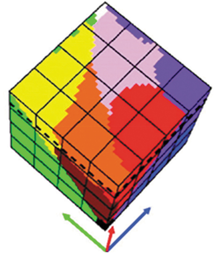
   2. Secondary/subordinate color information representation in the (2D) image-plane (refer to Subsection 4.1). In the multi-disciplinary domain of cognitive science (see Figure 11), an original contribution to color information representation in the cognitive process of (human) vision stems from linguistics (Ball, 2021).

      In their daily life, human beings, embodied in a 4D geospace-time physical world, adopt color naming, i.e. they call by name any numerical continuous color value (refer to Subsection 3.3.1), detected/sensed by an imaging sensor (specifically, the human eye) on an observed object’s surface in the 4D scene-domain and mapped retinotopically (refer to references listed in Section 2) onto a (2D) image-plane (see Figure 20). The color name mapped from (associated with) a sensed color value belongs to a nominal/categorical variable, i.e. it belongs to a discrete and finite vocabulary of color names, to be community-agreed upon for correct (conventional) interpretation, according to the notion of semantics-in-context (Ball, 2021), equivalent to meaning-by-convention (Santoro et al., 2021), well known in semiotics (refer to Section 2), before use by members of a community.

      In linguistics (Berlin & Kay, 1969), color naming is the capability of mapping numerical color values into a discrete and finite vocabulary of categorical basic color (BC) names, to be community-agreed upon for correct (conventional) interpretation before use by members of the community. Central to this consideration is Berlin and Kay’s landmark study in linguistics of a “universal” inventory of eleven BC words adopted in twenty human languages developed across geographical space and time: black, white, gray, red, orange, yellow, green, blue, purple, pink and brown (Berlin & Kay, 1969).

      To better understand the mathematical and physical meaning of color names (Boynton, 1990), let us observe that, first, BC names in human languages are mathematically equivalent to a latent/hidden categorical variable (Baraldi, 2017; Baraldi & Tiede, 2018a, 2018b; Shotton et al., 2009; Wikipedia, 2015), see Figure 15. Second, in human perception, BC names in human languages correspond to perceptual polyhedra (Benavente et al., 2008; Griffin, 2006; Parraga et al., 2009) providing a mutually exclusive and totally exhaustive partition of a monitor-typical color data cube (see Figure 29), whose three spectral dimensions are the visible Red-Green-Blue (RGB) channels, located in the visible portion of the electromagnetic spectrum, see Figures 7 and 8.

      Noteworthy, first, an RGB data cube polyhedralization into BC color names is intuitive to think of and easy to visualize, see Figure 29. Second, in an RGB color space, BC name-specific RGB polyhedra are neither necessarily convex nor connected, see Figure 29. Third, unlike an RGB data cube polyhedralization into BC color names, if the number of spectral channels is superior to three, then hyperpolyhedralization of a MS reflectance hyperspace into a discrete and finite vocabulary of hypercolor names is difficult to think of and impossible to visualize, see Figure 30. Fourth, no community-agreed vocabulary of hypercolor names exists in traditional human languages, since the human eye (see Figure 20), employed as visual data source, is sensitive exclusively to the visible RGB channels, located in the visible portion of the electromagnetic spectrum, see Figures 7 and 8. It means that, when required, like in the SIAM lightweight computer program (refer to references listed in Section 2), capable of deductive/prior knowledge-based MS reflectance space hyperpolyhedralization into a finite and discrete vocabulary of MS hypercolor names (see Figure 2 and Figure 30), where MS channels range from the visible to the thermal portion of the electromagnetic spectrum (see Figures 7 and 8), first, hypercolor names must be made up with (invented as) new words or phrases, not-yet existing in traditional human languages. Second, an invented vocabulary of hypercolor names, which never existed before in traditional human languages, must be community-agreed upon for correct (conventional) interpretation, according to the notion of semantics-in-context (Ball, 2021), equivalent to meaning-by-convention (Santoro et al., 2021), well known in semiotics (refer to Section 2), before use by members of a community, such as the RS community traditionally involved with EO optical (either PAN, MS, SS or HS) image interpretation, see Figure 7 and Figure 30.

      Figure 30. Unlike a 3-dimensional RGB true- or false-color data cube polyhedralization into RGB color names, which is intuitive to think of and straightforward to display (see Figure 29), a multi-spectral (MS) data space (hyper)polyhedralization into MS (hyper)color names is difficult to think of and impossible to visualize when the number of spectral channels is superior to three. As a possible example of hyperpolyhedron in a MS data hypercube, let us consider land cover (LC) class-specific (class-conditional) families of spectral signatures (Swain & Davis, 1978) in top-of-atmosphere reflectance (TOARF) values ∈ [0.0, 1.0], which include surface reflectance (SURF) values ∈ [0.0, 1.0] as a special case in clear sky and flat terrain conditions (Chavez, 1988), in agreement with Equation (8)(8) $\begin{array}{rl}& \text{lsquo}\mathrm{D}\mathrm{N}\mathrm{s}\ge 0\mathrm{a}\mathrm{t}\mathrm{E}\mathrm{O}\mathrm{L}\mathrm{e}\mathrm{v}\mathrm{e}\mathrm{l}0\supseteq \mathrm{T}\mathrm{O}\mathrm{A}\mathrm{R}\mathrm{F}\in \left[0.0,1.0\right]\mathrm{a}\mathrm{t}\mathrm{E}\mathrm{O}\mathrm{L}\mathrm{e}\mathrm{v}\mathrm{e}\mathrm{l}1\supseteq \mathrm{S}\mathrm{U}\mathrm{R}\mathrm{F}\in \left[0.0,1.0\right]\\ & \mathrm{a}\mathrm{t}\mathrm{E}\mathrm{O}\mathrm{L}\mathrm{e}\mathrm{v}\mathrm{e}\mathrm{l}2/\left(\mathrm{c}\mathrm{u}\mathrm{r}\mathrm{r}\mathrm{e}\mathrm{n}\mathrm{t}\right)\mathrm{A}\mathrm{R}\mathrm{D}\supseteq \mathrm{S}\mathrm{u}\mathrm{r}\mathrm{f}\mathrm{a}\mathrm{c}\mathrm{e}\mathrm{a}\mathrm{l}\mathrm{b}\mathrm{e}\mathrm{d}\mathrm{o}\in \left[0.0,1.0\right]\mathrm{a}\mathrm{t},\mathrm{s}\mathrm{a}\mathrm{y},\mathrm{E}\mathrm{O}\mathrm{L}\mathrm{e}\mathrm{v}\mathrm{e}\mathrm{l}3/\mathrm{n}\mathrm{e}\mathrm{x}\mathrm{t}\\ & \mathrm{g}\mathrm{e}\mathrm{n}\mathrm{e}\mathrm{r}\mathrm{a}\mathrm{t}\mathrm{i}\mathrm{o}\mathrm{n}\mathrm{A}\mathrm{R}\mathrm{D}\text{rsquo}& (8)\end{array}$(8) to Equation (11)(11) $\text{lsquo}\mathrm{T}\mathrm{O}\mathrm{A}\mathrm{R}\mathrm{F}\approx \mathrm{S}\mathrm{U}\mathrm{R}\mathrm{F}\text{rsquo}$(11) . A within-class family of spectral signatures (e.g. dark-toned soil) in Equation (8)(8) $\begin{array}{rl}& \text{lsquo}\mathrm{D}\mathrm{N}\mathrm{s}\ge 0\mathrm{a}\mathrm{t}\mathrm{E}\mathrm{O}\mathrm{L}\mathrm{e}\mathrm{v}\mathrm{e}\mathrm{l}0\supseteq \mathrm{T}\mathrm{O}\mathrm{A}\mathrm{R}\mathrm{F}\in \left[0.0,1.0\right]\mathrm{a}\mathrm{t}\mathrm{E}\mathrm{O}\mathrm{L}\mathrm{e}\mathrm{v}\mathrm{e}\mathrm{l}1\supseteq \mathrm{S}\mathrm{U}\mathrm{R}\mathrm{F}\in \left[0.0,1.0\right]\\ & \mathrm{a}\mathrm{t}\mathrm{E}\mathrm{O}\mathrm{L}\mathrm{e}\mathrm{v}\mathrm{e}\mathrm{l}2/\left(\mathrm{c}\mathrm{u}\mathrm{r}\mathrm{r}\mathrm{e}\mathrm{n}\mathrm{t}\right)\mathrm{A}\mathrm{R}\mathrm{D}\supseteq \mathrm{S}\mathrm{u}\mathrm{r}\mathrm{f}\mathrm{a}\mathrm{c}\mathrm{e}\mathrm{a}\mathrm{l}\mathrm{b}\mathrm{e}\mathrm{d}\mathrm{o}\in \left[0.0,1.0\right]\mathrm{a}\mathrm{t},\mathrm{s}\mathrm{a}\mathrm{y},\mathrm{E}\mathrm{O}\mathrm{L}\mathrm{e}\mathrm{v}\mathrm{e}\mathrm{l}3/\mathrm{n}\mathrm{e}\mathrm{x}\mathrm{t}\\ & \mathrm{g}\mathrm{e}\mathrm{n}\mathrm{e}\mathrm{r}\mathrm{a}\mathrm{t}\mathrm{i}\mathrm{o}\mathrm{n}\mathrm{A}\mathrm{R}\mathrm{D}\text{rsquo}& (8)\end{array}$(8) = ‘TOARF ⊇ SURF’ values forms a buffer zone/ hyperpolyhedron/ envelope/ manifold/ joint distribution, depicted in light green, where SURF values as special case of TOARF values are depicted by a red line. Like a vector quantity has two characteristics, a magnitude and a direction, any LC class-specific MS manifold/hyperpolyhedron is characterized by a multivariate shape information component and a multivariate intensity information component. In the RS literature, typical prior knowledge-based spectral decision trees for MS data space partitioning (hyperpolyhedralization) into a finite and discrete vocabulary of MS color names, such as those adopted in the European Space Agency (ESA) Sentinel 2 (atmospheric, topographic and adjacency) Correction Prototype Processor (Sen2Cor) (DLR – Deutsches Zentrum für Luft-und Raumfahrt e.V. and VEGA Technologies, 2011; ESA – European Space Agency, 2015), the Multisensor Atmospheric Correction and Cloud Screening (MACCS)-Atmospheric/Topographic Correction (ATCOR) Joint Algorithm (MAJA) (Hagolle et al., 2017; Main-Knorn et al., 2018), the ATCOR commercial software toolbox (Richter & Schläpfer, 2012), the U.S. Geological Survey (USGS)-National Aeronautics and Space Administration (NASA) Landsat Ecosystem Disturbance Adaptive Processing System (LEDAPS) for Landsat-4/-5/-7 imagery (Vermote & Saleous, 2007) and the Landsat Surface Reflectance Code (LaSRC) for Landsat-8 imagery (Bilal et al., 2019; Qiu et al., 2019; USGS – U.S. Geological Survey, 2018b), typically adopt either a multivariate analysis of a stack of two-band spectral indexes or a logical (AND, OR) combination of univariate analyses (typically, scalar variable thresholding), where scalar spectral indexes or scalar spectral channels are analysed individually as univariate variables (Adamo et al., 2020; DLR – Deutsches Zentrum für Luft-und Raumfahrt e.V. and VEGA Technologies, 2011; ESA – European Space Agency, 2015; Gao, 1996; Goffi et al., 2020; Huth, Kuenzer, Wehrmann, Gebhardt, & Dech, 2012; Jordan, 1969; Kang Lee et al., 2018; Kashongwe et al., 2020; Key & Benson, 1999; Liang, 2004; Lozano et al., 2007; Marconcini et al., 2020; McFeeters, 1996; Neduni & Sivakumar, 2019; Rouse et al., 1974; Roy et al., 2009; Sykas, 2020; Tucker, 1979; Xu, 2006). A typical two-band spectral index is a scalar band ratio or band-pair difference equivalent to an angular coefficient (1^st-order derivative) of a tangent to the spectral signature in one point, see Figure 7 and Table 3. It is well known that infinite functions can feature the same tangent value in one point. In practice, unlike combinations of basis functions working as universal approximators (Bishop, 1995; Cherkassky & Mulier, 1998), no combination of spectral indexes can reconstruct the multivariate shape and multivariate intensity information components of a spectral signature, see Figure 7. As viable alternative to traditional static (non-adaptive to data) spectral rule-based decision trees for MS color naming found in the RS literature, based on thresholding either scalar spectral channels or scalar spectral indexes (Liang, 2004) (see Table 3), such as the per-pixel decision tree implemented by the ESA Level 2 Sentinel-2 (atmospheric, adjacency and topographic) Correction Prototype Processor (Sen2Cor) software toolbox for Scene Classification Map (SCM) generation (DLR – Deutsches Zentrum für Luft-und Raumfahrt e.V. and VEGA Technologies, 2011; ESA – European Space Agency, 2015), the Satellite Image Automatic Mapper (SIAM)’s prior knowledge-based spectral decision tree (Baraldi, 2017, 2019a; Baraldi et al., 2010a, 2010b, 2018a, 2018b, 2006; Baraldi & Tiede, 2018a, 2018b) adopts a convergence-of-evidence approach to model any target family (ensemble) of spectral signatures, forming a hyperpolyhedron of interest in the MS reflectance hyperspace, as a combination of a multivariate shape information component with a multivariate intensity information component. For example, as shown above, typical spectral signatures of dark-toned soils and typical spectral signatures of light-toned soils form two MS envelopes in the MS reflectance hyperspace that approximately share the same multivariate shape information component, but whose pair of multivariate intensity information components does differ.

      

      Per se (on a standalone basis), color naming transforms/maps a numerical (either continuous or discrete, refer to Subsection 3.3.1) multi-variate/chromatic/color image/2D gridded data into a multi-level/categorical image (Sonka et al., 1994), where the output number of detected image-levels ranges from one to the cardinality of the discrete and finite vocabulary of color names, see Figure 31(a).

      Worth mentioning, whereas traditional numerical image segmentation/partitioning is an inherently ill-posed cognitive (perceptual) problem (Vecera & Farah, 1997) (refer to Subsection 4.1), multi-level/categorical image segmentation/partitioning is a well-posed/deterministic problem, whose solution is unique/unequivocal (Baraldi, 2017; Dillencourt et al., 1992; Hadamard, 1902; Sonka et al., 1994), see Figure 31(a). To accomplish the deterministic task of segmentation map generation from a multi-level/categorical image, the well-known two-pass connected-component multi-level image labeling algorithm (Dillencourt et al., 1992; Sonka et al., 1994) is deterministic/well-posed (admits a single solution), automatic (it requires no human-machine interaction, i.e. there is no model’s hyperparameter to be user-defined based on heuristics, refer to Subsection 3.1) and demands two raster scans of the input multi-level 2D gridded data (see Figure 31(a)); hence, its computational complexity increases linearly (as best case of polynomial complexity) with image size (refer to Subsection 3.1).

      The observed simplification of an image segmentation problem, from inherently ill-posed 2D gridded numerical variable partitioning to well-posed 2D gridded categorical variable partitioning in linear computational complexity, shows the methodological and practical relevance of the categorization/discretization process of mapping subsymbolic sensory data (input numerical variables), either continuous or discrete (refer to Section 3.3.1), into hidden (discrete and finite, either subsymbolic or semi-symbolic, refer to Section 3.3.1) categorical variables as intermediate stage (see Figure 15) in the inherently ill-posed cognitive process of symbolic (categorical and semantic, refer to Section 3.3.1) interpretation/ classification/ understanding (refer to Section 2) of (numerical) sensory data, whose special case is the cognitive/interpretation process of vision, synonym for inherently ill-posed 4D scene-from-(2D) image reconstruction and understanding, see Figure 20.

5. Marr levels of system understanding 2-of-5 to 4-of-5 (refer to Subsection 3.2): Information/knowledge representation, system design and algorithm. In psychophysics, recent studies on human visual perception revealed that mental imagery is capable of inducing a retinotopically organized (2D spatial topology preserving) activation of early (retinal) visual areas via feedback connections, from mind back to sensor (see Figure 20), which is tantamount to saying that “mental images in the mind’s eye can alter the way we see things in the retina” (Slotnick et al., 2005) (refer to Subsection 4.1). This evidence means that, to make an inherently ill-posed ‘CV ⊃ EO-IU’ system better posed for numerical solution (refer to references listed in Subsection 3.3.2) by reverse engineering human visual perception (see Figure 26), a source of a priori knowledge, available in addition to 2D sensory data (imagery), is a 7D conceptual (mental) world model, which is expected to be stable/hard-to-vary (Sweeney, 2018a), but also plastic (self-organizing, capable of incremental learning to model non-stationary data distributions) (refer to Subsection 3.3.4), to be involved with a mind-to-sensor feedback projection mechanism, see Figure 20.

   In Subsection 4.1, an example of mind-to-sensor feedback projection (see Figure 20) involved a 7D mental world model, in user-speak, back-projected onto a (2D) image-plane, in techno-speak, once the imaging sensor’s spatial and spectral resolution specifications are also known a priori, see Figure 8.

   Noteworthy, a feedback system architecture is alternative to feedforward inference systems, such as popular ‘DCNN ⊂ DL ⊂ ML’ solutions (Cimpoi et al., 2014; Krizhevsky et al., 2012).

6. Marr levels of system understanding 3-of-5 and 4-of-5 (refer to Subsection 3.2): System design (architecture) and algorithm. A ‘CV ⊃ EO-IU’ system architecture is required to:

   1. Comply with the structured system design principles (Page-Jones, 1988), such as the modularity, hierarchy and regularity criteria recommended for system scalability (Lipson, 2007), in agreement with the FAIR criteria (GO FAIR – International Support and Coordination Office, 2021; Wilkinson et al., 2016) (refer to Subsection 3.5) and with a popular divide-and-conquer (divide-et-impera) problem solving approach (Baraldi, 2017; Baraldi & Tiede, 2018a, 2018b; Bishop, 1995; Cherkassky & Mulier, 1998), where a difficult problem is divided into subproblems easier to be coped with.

      For example, a hierarchical modular approach is required to form neural modularity systems, equivalent to a hierarchical modular network (distributed processing system) of component networks/subnetworks (Baraldi, 2017; Baraldi & Tiede, 2018a, 2018b; DiCarlo, 2017; Kosslyn, 1994; Rappe, 2018; Slotnick et al., 2005; Tsotsos, 1990; Vecera & Farah, 1997). Networks of component networks consist of synaptic connections, either lateral (intra-layer) connections or vertical (inter-layer) connections, where vertical links can be either feed-forward or feed-back connections. Their processing units cooperate (e.g. intra-layer), but also compete to form specialized subnetworks, i.e. network specialization is accomplished through neural competition mechanisms (Baraldi & Alpaydin, 2002a, 2002b; Fritzke, 1997; Martinetz et al., 1994). Structured system design principles (Page-Jones, 1988), aiming at the development of specialized component systems (e.g. component networks specialized through competition) that cooperate in a system of component systems (e.g. a network of specialized component networks), cope with the so-called “black box” problem affecting traditional ANNs (Baraldi & Tiede, 2018a, 2018b; Marcus, 2018, 2020; Salmon, 1963), including DCNNs (Cimpoi et al., 2014; Krizhevsky et al., 2012), synonym for low interpretability/ traceability/ accountability/ explainability (Koehrsen, 2018; Lukianoff, 2019) (refer to Subsection 3.1).

      Figure 31. One segmentation map is deterministically generated from one multi-level (e.g. binary) image, such as a thematic map, but the vice versa does not hold, i.e. many multi-level images can generate the same segmentation map. (a) To accomplish the deterministic task of segmentation map generation from a multi-level image, the two-pass connected-component multi-level image labeling algorithm (Dillencourt et al., 1992; Sonka et al., 1994) requires two raster scans of the input data set. In the figure above, as an example, nine image-objects/segments S1 to S9 can be detected in the 3-level thematic map shown at left. (b) Example of a 4-adjacency cross-aura map, shown at right, where 4-adjacency cross-aura values belong to range {0, 4}, generated in linear time from a multi-level image, such as a two-level image, shown at left. In addition to depicting image-object contours for qualitative visual assessment, these 4-adjacency contour values are suitable for shape index estimation, such as scale-invariant roundness (compactness and no holiness) in range [0.0, 1.0] (Baraldi, 2017; Baraldi & Soares, 2017).

      

   2. Be provided with inter-module feedback loops (Baraldi, 2017; Baraldi & Tiede, 2018a, 2018b; DiCarlo, 2017; Hawkins, 2021; Hawkins et al., 2017; Kosslyn, 1994; Rappe, 2018; Slotnick et al., 2005; Tsotsos, 1990; Vecera & Farah, 1997). As reported in this Subsection above, directed feedback connections can map (back-project) information/knowledge from the high-level inference system (mind), modulated by (filtered by) the technical specifications of the imaging sensor (eye), to the low-level (2D) image-plane (retina), in agreement with psychophysical evidence about human mental images (Slotnick et al., 2005), see Figure 20. A feedback system architecture is alternative to feedforward inference systems, such as popular ‘DCNN ⊂ DL ⊂ ML’ solutions (Cimpoi et al., 2014; Krizhevsky et al., 2012).

   3. Adopt a convergence-of-evidence approach, consistent with human reasoning (Baraldi, 2017; Green et al., 2002; Kuhn, 2005; Laurini & Thompson, 1992; Matsuyama & Hwang, 1990; Newell & Simon, 1972; Sheth, 2015; Sonka et al., 1994; Sowa, 2000), where weak, but statistically independent sources of evidence (refer to Section 2) suffice to infer strong conjectures (Baraldi, 2017; Matsuyama & Hwang, 1990; Nagao & Matsuyama, 1980).

      An original formulation of a convergence-of-evidence approach to inherently ill-posed ‘CV ⊃ EO-IU ⊃ ARD’ problems (Matsuyama & Hwang, 1990; Nagao & Matsuyama, 1980), where a priori knowledge is required in addition to data (features, either sensory data and/or sensory data-derived numerical or categorical variables, refer to Subsection 3.3.1) to become better posed for numerical solution (refer to references listed in Subsection 3.3.2), is presented below (Baraldi, 2017; Baraldi et al., 2018a, 2018b; Baraldi & Tiede, 2018a, 2018b), in compliance with a well-known naïve Bayes probabilistic classification framework, based on applying Bayes’ theorem with strong (naïve) statistical independence assumptions (refer to Section 2) about input features (numerical variables, information components, sources of evidence) (Bishop, 1995; Cherkassky & Mulier, 1998).

      According to semantic relationship ‘Cognitive science ⊃ AGI ⊃ CV ⊃ EO-IU ⊃ ARD’ = Equation (3)(3) $\text{lsquo}\mathrm{A}\mathrm{R}\mathrm{D}\subset \mathrm{E}\mathrm{O}-\mathrm{I}\mathrm{U}\subset \mathrm{C}\mathrm{V}\subset \mathrm{A}\mathrm{G}\mathrm{I}\subset \mathrm{C}\mathrm{o}\mathrm{g}\mathrm{n}\mathrm{i}\mathrm{t}\mathrm{i}\mathrm{v}\mathrm{e}\mathrm{s}\mathrm{c}\mathrm{i}\mathrm{e}\mathrm{n}\mathrm{c}\mathrm{e}\text{rsquo}$(3) , in the cognitive subdomain of ‘CV ⊃ EO-IU ⊃ ARD’ problems, a stable/hard-to-vary 7D conceptual (mental) world model (refer to Subsection 3.3.4), whose part-of is a discrete and finite set/ vocabulary/ taxonomy of entities, identified hereafter as ObjectClassLegend = {ObjectClass_c, c = 1, …, ObjectClassLegendCardinality}, is available a priori in addition to data (observations, true-facts). For any observation (true-fact) x identified by a CV system in the (2D) image-plane (see Figure 20), where x is a 2D spatial unit (Wikipedia, 2014a, 2014b), either 0D pixel, 1D line or 2D polygon according to the OGC nomenclature (OGC – Open Geospatial Consortium Inc, 2015), an original formulation of the well-known naïve Bayes probabilistic classifier (Bishop, 1995; Cherkassky & Mulier, 1998) is proposed hereafter, capable of a convergence-of-evidence approach to inherently ill-posed ‘CV ⊃ EO-IU ⊃ ARD’ cognitive tasks (see Figure 20) where, first, 2D spatial and colorimetric information components (sources of evidence, features) in the (2D) image-plane are statistically independent (refer to Subsection 4.1) and, second, a discrete and finite vocabulary of color names (refer to this Subsection above) is employed as latent/hidden categorical variable, in agreement with Figure 15. In the proposed formulation of a naïve Bayes probabilistic classifier of spatial unit x ∈ (2D) image-plane, an ObjectClass_c-specific posterior probability is computed as

   p(c | ColorValue(x) = z ∈ ℜ^MS, SizeValue(x), 2DshapeValue(x), TextureValue(x), 2DspatialRelationships(x, 2Dneigh(x))) = 

   $\begin{array}{rl}& \mathrm{p}(\mathrm{c}|\mathrm{C}\mathrm{o}\mathrm{l}\mathrm{o}\mathrm{r}\mathrm{V}\mathrm{a}\mathrm{l}\mathrm{u}\mathrm{e}\left(\mathrm{x}\right)=\mathrm{z}\in {\mathrm{\Re }}^{\mathrm{M}\mathrm{S}},\mathrm{S}\mathrm{i}\mathrm{z}\mathrm{e}\mathrm{V}\mathrm{a}\mathrm{l}\mathrm{u}\mathrm{e}\left(\mathrm{x}\right),2\mathrm{D}\mathrm{s}\mathrm{h}\mathrm{a}\mathrm{p}\mathrm{e}\mathrm{V}\mathrm{a}\mathrm{l}\mathrm{u}\mathrm{e}\left(\mathrm{x}\right),\\ & \mathrm{T}\mathrm{e}\mathrm{x}\mathrm{t}\mathrm{u}\mathrm{r}\mathrm{e}\mathrm{V}\mathrm{a}\mathrm{l}\mathrm{u}\mathrm{e}\left(\mathrm{x}\right),2\mathrm{D}\mathrm{s}\mathrm{p}\mathrm{a}\mathrm{t}\mathrm{i}\mathrm{a}\mathrm{l}\mathrm{R}\mathrm{e}\mathrm{l}\mathrm{a}\mathrm{t}\mathrm{i}\mathrm{o}\mathrm{n}\mathrm{s}\mathrm{h}\mathrm{i}\mathrm{p}\mathrm{s}\left(\mathrm{x},2\mathrm{D}\mathrm{n}\mathrm{e}\mathrm{i}\mathrm{g}\mathrm{h}\left(\mathrm{x}\right)\right))\\ & =\mathrm{p}\left(\mathrm{c}|{\mathrm{F}}_1,\dots ,{\mathrm{F}}_5\right)=\mathrm{p}\left(\mathrm{c}\right){\prod }_{i=1}^{I=5}p\left({\mathrm{F}}_{\mathrm{i}}|\mathrm{c}\right)\propto {\prod }_{i=1}^{I=5}p\left(F_i|c\right),\end{array}$

   where 2D spatial and colorimetric features F_i, with i = 1, …, 5, are statistically independent (refer to Subsection 4.1) and where

   $x0026;{\displaystyle {\prod }_{i=1}^{I=5}p}\left({\text{F}}_{\text{i}}\text{|c}\right)\text{=p}\left(\text{ColorValue}\left(\text{x}\right)\text{|c}\right)\times \text{p}\left(\text{SizeValue}\left(\text{x}\right)\text{|c}\right)\times \text{p}x0026;\left(\text{2DshapeValue}\left(\text{x}\right)\text{|c}\right)\times \text{p}\left(\text{TextureValue}\left(\text{x}\right)\text{|c}\right)\times \text{p}(\text{2DspatialRelationships}x0026;\left(\text{x},\text{2Dneigh}\left(\text{x}\right)\right)\text{|c}={\displaystyle \sum _{{\text{ColorName}}_j,\text{e}.\text{g}.,\text{Red},\text{Green},\text{Blue},\text{etc}.,\text{with}\text{j}=1}^{\text{ColorVocabularyCardinality}}}x0026;\text{p}\left(\text{ColorValue}\left(\text{x}\right){\text{|ColorName}}_{\text{j}}\right)\times \text{p}\left({\text{ColorName}}_{\text{j}}\text{|c}\right)\times x0026;\text{p}\left(\text{SizeValue}\left(\text{x}\right)\text{|c}\right)\times \text{p}\left(\text{2DshapeValue}\left(\text{x}\right)\text{|c}\right)\times \text{p}\left(\text{TextureValue}\left(\text{x}\right)\text{|c}\right)\times x0026;\text{p}\left(\text{2DspatialRelationships}\left(\text{x},\text{2Dneigh}\left(\text{x}\right)\right)\text{|c}\right)$

   with c = 1, …, ObjectClassLegendCardinality in the adopted 7D conceptual world model (refer to Subsection 3.3.4).

   When a probability function, p(⋅) ∈ [0.0, 1.0], in the frequentist view of probability, is transformed onto a notion of membership/compatibility function, m(⋅) ∈ [0.0, 1.0], according to principles of fuzzy logic (Zadeh, 1965), then the product of statistically independent probability values is replaced by the Fuzzy-AND operator = MIN operation among membership/compatibility values. Hence, the equation above becomes:$\begin{array}{rl}& m(c|ColorValue\left(x\right)=z\in {\mathrm{\Re }}^{MS},SizeValue\left(x\right),2DshapeValue\left(x\right),\\ & TextureValue\left(x\right),2DspatialRelationships\left(x,2Dneigh\left(x\right)\right))\propto \end{array}$

   (12) $\begin{array}{rl}& \mathrm{M}\mathrm{I}\mathrm{N}\left\{\begin{array}{c}\mathrm{m}\left(\mathrm{C}\mathrm{o}\mathrm{l}\mathrm{o}\mathrm{r}\mathrm{V}\mathrm{a}\mathrm{l}\mathrm{u}\mathrm{e}\left(\mathrm{x}\right)|\mathrm{c}\right),\mathrm{m}\left(\mathrm{S}\mathrm{i}\mathrm{z}\mathrm{e}\mathrm{V}\mathrm{a}\mathrm{l}\mathrm{u}\mathrm{e}\left(\mathrm{x}\right)|\mathrm{c}\right),\\ \mathrm{m}\left(2\mathrm{D}\mathrm{s}\mathrm{h}\mathrm{a}\mathrm{p}\mathrm{e}\mathrm{V}\mathrm{a}\mathrm{l}\mathrm{u}\mathrm{e}\left(\mathrm{x}\right)|\mathrm{c}\right),\mathrm{m}\left(\mathrm{T}\mathrm{e}\mathrm{x}\mathrm{t}\mathrm{u}\mathrm{r}\mathrm{e}\mathrm{V}\mathrm{a}\mathrm{l}\mathrm{u}\mathrm{e}\left(\mathrm{x}\right)|\mathrm{c}\right),\\ \mathrm{m}\left(2\mathrm{D}\mathrm{s}\mathrm{p}\mathrm{a}\mathrm{t}\mathrm{i}\mathrm{a}\mathrm{l}\mathrm{R}\mathrm{e}\mathrm{l}\mathrm{a}\mathrm{t}\mathrm{i}\mathrm{o}\mathrm{n}\mathrm{s}\mathrm{h}\mathrm{i}\mathrm{p}\mathrm{s}\left(\mathrm{x},2\mathrm{D}\mathrm{n}\mathrm{e}\mathrm{i}\mathrm{g}\mathrm{h}\left(\mathrm{x}\right)\right)|\mathrm{c}\right)\end{array}\right\}\\ & =\mathrm{M}\mathrm{I}\mathrm{N}\left\{\begin{array}{c}\sum _{\mathrm{C}\mathrm{o}\mathrm{l}\mathrm{o}\mathrm{r}\mathrm{N}\mathrm{a}\mathrm{m}{\mathrm{e}}_{\mathrm{j}},\mathrm{e}.\mathrm{g}.,\mathrm{r}\mathrm{e}\mathrm{d},\mathrm{g}\mathrm{r}\mathrm{e}\mathrm{e}\mathrm{n},\mathrm{b}\mathrm{l}\mathrm{u}\mathrm{e},\mathrm{e}\mathrm{t}\mathrm{c}.,\mathrm{w}\mathrm{i}\mathrm{t}\mathrm{h}\mathrm{j}=1}^{\mathrm{C}\mathrm{o}\mathrm{l}\mathrm{o}\mathrm{r}\mathrm{V}\mathrm{o}\mathrm{c}\mathrm{a}\mathrm{b}\mathrm{u}\mathrm{l}\mathrm{a}\mathrm{r}\mathrm{y}\mathrm{C}\mathrm{a}\mathrm{r}\mathrm{d}\mathrm{i}\mathrm{n}\mathrm{a}\mathrm{l}\mathrm{i}\mathrm{t}\mathrm{y}}\\ \mathrm{m}\left(\mathrm{C}\mathrm{o}\mathrm{l}\mathrm{o}\mathrm{r}\mathrm{V}\mathrm{a}\mathrm{l}\mathrm{u}\mathrm{e}\left(\mathrm{x}\right)|\mathrm{C}\mathrm{o}\mathrm{l}\mathrm{o}\mathrm{r}\mathrm{N}\mathrm{a}\mathrm{m}{\mathrm{e}}_{\mathrm{j}}\right)\mathrm{m}\left(\mathrm{C}\mathrm{o}\mathrm{l}\mathrm{o}\mathrm{r}\mathrm{N}\mathrm{a}\mathrm{m}{\mathrm{e}}_{\mathrm{j}}|\mathrm{c}\right),\\ \mathrm{m}\left(\mathrm{S}\mathrm{i}\mathrm{z}\mathrm{e}\mathrm{V}\mathrm{a}\mathrm{l}\mathrm{u}\mathrm{e}\left(\mathrm{x}\right)|\mathrm{c}\right),\mathrm{m}\left(2\mathrm{D}\mathrm{s}\mathrm{h}\mathrm{a}\mathrm{p}\mathrm{e}\mathrm{V}\mathrm{a}\mathrm{l}\mathrm{u}\mathrm{e}\left(\mathrm{x}\right)|\mathrm{c}\right),\\ \mathrm{m}\left(\mathrm{T}\mathrm{e}\mathrm{x}\mathrm{t}\mathrm{u}\mathrm{r}\mathrm{e}\mathrm{V}\mathrm{a}\mathrm{l}\mathrm{u}\mathrm{e}\left(\mathrm{x}\right)|\mathrm{c}\right),\\ \mathrm{m}\left(2\mathrm{D}\mathrm{s}\mathrm{p}\mathrm{a}\mathrm{t}\mathrm{i}\mathrm{a}\mathrm{l}\mathrm{R}\mathrm{e}\mathrm{l}\mathrm{a}\mathrm{t}\mathrm{i}\mathrm{o}\mathrm{n}\mathrm{s}\mathrm{h}\mathrm{i}\mathrm{p}\mathrm{s}\left(\mathrm{x},2\mathrm{D}\mathrm{n}\mathrm{e}\mathrm{i}\mathrm{g}\mathrm{h}\left(\mathrm{x}\right)\right)|\mathrm{c}\right)\end{array}\right\}\\ & =\mathrm{M}\mathrm{I}\mathrm{N}\{\mathrm{m}\left(\mathrm{C}\mathrm{o}\mathrm{l}\mathrm{o}\mathrm{r}\mathrm{N}\mathrm{a}\mathrm{m}{\mathrm{e}}^{\ast }|\mathrm{c}\right)\in \left\{0,1\right\},\mathrm{m}\left(\mathrm{S}\mathrm{i}\mathrm{z}\mathrm{e}\mathrm{V}\mathrm{a}\mathrm{l}\mathrm{u}\mathrm{e}\left(\mathrm{x}\right)|\mathrm{c}\right)\in \left[0.0,1.0\right],\\ & \mathrm{m}\left(2\mathrm{D}\mathrm{s}\mathrm{h}\mathrm{a}\mathrm{p}\mathrm{e}\mathrm{V}\mathrm{a}\mathrm{l}\mathrm{u}\mathrm{e}\left(\mathrm{x}\right)|\mathrm{c}\right)\in \left[0.0,1.0\right],\mathrm{m}\left(\mathrm{T}\mathrm{e}\mathrm{x}\mathrm{t}\mathrm{u}\mathrm{r}\mathrm{e}\mathrm{V}\mathrm{a}\mathrm{l}\mathrm{u}\mathrm{e}\left(\mathrm{x}\right)|\mathrm{c}\right)\in \left[0.0,1.0\right],\\ & \mathrm{m}\left(2\mathrm{D}\mathrm{s}\mathrm{p}\mathrm{a}\mathrm{t}\mathrm{i}\mathrm{a}\mathrm{l}\mathrm{R}\mathrm{e}\mathrm{l}\mathrm{a}\mathrm{t}\mathrm{i}\mathrm{o}\mathrm{n}\mathrm{s}\mathrm{h}\mathrm{i}\mathrm{p}\mathrm{s}\left(\mathrm{x},2\mathrm{D}\mathrm{n}\mathrm{e}\mathrm{i}\mathrm{g}\mathrm{h}\left(\mathrm{x}\right)\right)|\mathrm{c}\right)\in \left[0.0,1.0\right]\}\end{array}$(12)

   where

   • x is a spatial unit in the (2D) image-plane, either 0D pixel, 1D line or 2D polygon according to the OGC nomenclature (OGC – Open Geospatial Consortium Inc, 2015).

   • • c = 1, …, ObjectClassLegendCardinality in the adopted 7D conceptual world model, available a priori (refer to Subsection 3.3.4).

   • • ColorValue(x) = z ∈ ℜ^MS, where ℜ^MS is a MS data (hyper)space, whose dimensionality in spectral channels is MS ≥ 2 (refer to Section 2), see Figure 7, Figure 8, Figure 15, Figure 29 and Figure 30.

   • •ColorName* = “winning” ColorName* = ColorName_j* ∈ VocabularyOfColorNames = {ColorName_j, j = 1, ColorVocabularyCardinality}, it is the only ColorName_j*, corresponding to hyperpolyhedron_j* ⊂ ℜ^MS (see Figure 15, Figure 29 and Figure 30), where condition m(ColorValue(x) | ColorName*) = 1 holds, i.e. it is the sole ColorName_j* whose hyperpolyhedron_j* ⊂ ℜ^MS includes ColorValue(x) = z ∈ ℜ^MS.

     At the Marr level of system understanding 4-of-5 (refer to Subsection 3.2), namely, algorithm, for any given ColorValue(x) = z ∈ ℜ^MS, the winning ColorName* = ColorName_j*, whose hyperpolyhedron_j* ⊂ ℜ^MS includes ColorValue(x), is identified by a deterministic (well-posed) prior knowledge-based (static, non-adaptive to input data) color naming decision tree, such as SIAM (refer to references listed in Section 2), whose computational complexity increases linearly with ColorVocabularyCardinality and image size; hence, a well-posed prior knowledge-based color naming decision-tree algorithm can be considered near real-time.

   • • m(ColorName*| c) ∈ {0, 1} is a binary compatibility value, belonging to binary relationship R: A ⇒ B ⊆ A × B from set A = VocabularyOfColorNames = {ColorName_j, j = 1, …, ColorVocabularyCardinality} to set B = ObjectClassLegend = {ObjectClass_c, c = 1, …, ObjectClassLegendCardinality}, to be known a priori as part-of the adopted 7D conceptual world model, i.e. this binary relationship must be known before (in addition to) looking at spatial unit x in the (2D) image-plane, see Figure 32.

     In practice, for a given discrete and finite set/ vocabulary/ taxonomy of entities, identified as ObjectClassLegend = {ObjectClass_c, c = 1, …, ObjectClassLegendCardinality}, known a priori as part-of the adopted 7D conceptual/ mental/ perceptual world model (refer to Subsection 3.3.4) and graphically represented as a set of nodes in a semantic network (refer to Section 2), any ObjectClass_c-specific colorimetric attribute is defined as a categorical/nominal variable, consisting of the (discrete and finite) color names known a priori as being compatible with entity ObjectClass_c, with c = 1, …, ObjectClassLegendCardinality, see Figure 32.

To recap, in the application domain of Equation (3)(3) $\text{lsquo}\mathrm{A}\mathrm{R}\mathrm{D}\subset \mathrm{E}\mathrm{O}-\mathrm{I}\mathrm{U}\subset \mathrm{C}\mathrm{V}\subset \mathrm{A}\mathrm{G}\mathrm{I}\subset \mathrm{C}\mathrm{o}\mathrm{g}\mathrm{n}\mathrm{i}\mathrm{t}\mathrm{i}\mathrm{v}\mathrm{e}\mathrm{s}\mathrm{c}\mathrm{i}\mathrm{e}\mathrm{n}\mathrm{c}\mathrm{e}\text{rsquo}$(3) = ‘Cognitive science ⊃ AGI ⊃ CV ⊃ EO-IU ⊃ ARD’, Equation (12)(12) $\begin{array}{rl}& \mathrm{M}\mathrm{I}\mathrm{N}\left\{\begin{array}{c}\mathrm{m}\left(\mathrm{C}\mathrm{o}\mathrm{l}\mathrm{o}\mathrm{r}\mathrm{V}\mathrm{a}\mathrm{l}\mathrm{u}\mathrm{e}\left(\mathrm{x}\right)|\mathrm{c}\right),\mathrm{m}\left(\mathrm{S}\mathrm{i}\mathrm{z}\mathrm{e}\mathrm{V}\mathrm{a}\mathrm{l}\mathrm{u}\mathrm{e}\left(\mathrm{x}\right)|\mathrm{c}\right),\\ \mathrm{m}\left(2\mathrm{D}\mathrm{s}\mathrm{h}\mathrm{a}\mathrm{p}\mathrm{e}\mathrm{V}\mathrm{a}\mathrm{l}\mathrm{u}\mathrm{e}\left(\mathrm{x}\right)|\mathrm{c}\right),\mathrm{m}\left(\mathrm{T}\mathrm{e}\mathrm{x}\mathrm{t}\mathrm{u}\mathrm{r}\mathrm{e}\mathrm{V}\mathrm{a}\mathrm{l}\mathrm{u}\mathrm{e}\left(\mathrm{x}\right)|\mathrm{c}\right),\\ \mathrm{m}\left(2\mathrm{D}\mathrm{s}\mathrm{p}\mathrm{a}\mathrm{t}\mathrm{i}\mathrm{a}\mathrm{l}\mathrm{R}\mathrm{e}\mathrm{l}\mathrm{a}\mathrm{t}\mathrm{i}\mathrm{o}\mathrm{n}\mathrm{s}\mathrm{h}\mathrm{i}\mathrm{p}\mathrm{s}\left(\mathrm{x},2\mathrm{D}\mathrm{n}\mathrm{e}\mathrm{i}\mathrm{g}\mathrm{h}\left(\mathrm{x}\right)\right)|\mathrm{c}\right)\end{array}\right\}\\ & =\mathrm{M}\mathrm{I}\mathrm{N}\left\{\begin{array}{c}\sum _{\mathrm{C}\mathrm{o}\mathrm{l}\mathrm{o}\mathrm{r}\mathrm{N}\mathrm{a}\mathrm{m}{\mathrm{e}}_{\mathrm{j}},\mathrm{e}.\mathrm{g}.,\mathrm{r}\mathrm{e}\mathrm{d},\mathrm{g}\mathrm{r}\mathrm{e}\mathrm{e}\mathrm{n},\mathrm{b}\mathrm{l}\mathrm{u}\mathrm{e},\mathrm{e}\mathrm{t}\mathrm{c}.,\mathrm{w}\mathrm{i}\mathrm{t}\mathrm{h}\mathrm{j}=1}^{\mathrm{C}\mathrm{o}\mathrm{l}\mathrm{o}\mathrm{r}\mathrm{V}\mathrm{o}\mathrm{c}\mathrm{a}\mathrm{b}\mathrm{u}\mathrm{l}\mathrm{a}\mathrm{r}\mathrm{y}\mathrm{C}\mathrm{a}\mathrm{r}\mathrm{d}\mathrm{i}\mathrm{n}\mathrm{a}\mathrm{l}\mathrm{i}\mathrm{t}\mathrm{y}}\\ \mathrm{m}\left(\mathrm{C}\mathrm{o}\mathrm{l}\mathrm{o}\mathrm{r}\mathrm{V}\mathrm{a}\mathrm{l}\mathrm{u}\mathrm{e}\left(\mathrm{x}\right)|\mathrm{C}\mathrm{o}\mathrm{l}\mathrm{o}\mathrm{r}\mathrm{N}\mathrm{a}\mathrm{m}{\mathrm{e}}_{\mathrm{j}}\right)\mathrm{m}\left(\mathrm{C}\mathrm{o}\mathrm{l}\mathrm{o}\mathrm{r}\mathrm{N}\mathrm{a}\mathrm{m}{\mathrm{e}}_{\mathrm{j}}|\mathrm{c}\right),\\ \mathrm{m}\left(\mathrm{S}\mathrm{i}\mathrm{z}\mathrm{e}\mathrm{V}\mathrm{a}\mathrm{l}\mathrm{u}\mathrm{e}\left(\mathrm{x}\right)|\mathrm{c}\right),\mathrm{m}\left(2\mathrm{D}\mathrm{s}\mathrm{h}\mathrm{a}\mathrm{p}\mathrm{e}\mathrm{V}\mathrm{a}\mathrm{l}\mathrm{u}\mathrm{e}\left(\mathrm{x}\right)|\mathrm{c}\right),\\ \mathrm{m}\left(\mathrm{T}\mathrm{e}\mathrm{x}\mathrm{t}\mathrm{u}\mathrm{r}\mathrm{e}\mathrm{V}\mathrm{a}\mathrm{l}\mathrm{u}\mathrm{e}\left(\mathrm{x}\right)|\mathrm{c}\right),\\ \mathrm{m}\left(2\mathrm{D}\mathrm{s}\mathrm{p}\mathrm{a}\mathrm{t}\mathrm{i}\mathrm{a}\mathrm{l}\mathrm{R}\mathrm{e}\mathrm{l}\mathrm{a}\mathrm{t}\mathrm{i}\mathrm{o}\mathrm{n}\mathrm{s}\mathrm{h}\mathrm{i}\mathrm{p}\mathrm{s}\left(\mathrm{x},2\mathrm{D}\mathrm{n}\mathrm{e}\mathrm{i}\mathrm{g}\mathrm{h}\left(\mathrm{x}\right)\right)|\mathrm{c}\right)\end{array}\right\}\\ & =\mathrm{M}\mathrm{I}\mathrm{N}\{\mathrm{m}\left(\mathrm{C}\mathrm{o}\mathrm{l}\mathrm{o}\mathrm{r}\mathrm{N}\mathrm{a}\mathrm{m}{\mathrm{e}}^{\ast }|\mathrm{c}\right)\in \left\{0,1\right\},\mathrm{m}\left(\mathrm{S}\mathrm{i}\mathrm{z}\mathrm{e}\mathrm{V}\mathrm{a}\mathrm{l}\mathrm{u}\mathrm{e}\left(\mathrm{x}\right)|\mathrm{c}\right)\in \left[0.0,1.0\right],\\ & \mathrm{m}\left(2\mathrm{D}\mathrm{s}\mathrm{h}\mathrm{a}\mathrm{p}\mathrm{e}\mathrm{V}\mathrm{a}\mathrm{l}\mathrm{u}\mathrm{e}\left(\mathrm{x}\right)|\mathrm{c}\right)\in \left[0.0,1.0\right],\mathrm{m}\left(\mathrm{T}\mathrm{e}\mathrm{x}\mathrm{t}\mathrm{u}\mathrm{r}\mathrm{e}\mathrm{V}\mathrm{a}\mathrm{l}\mathrm{u}\mathrm{e}\left(\mathrm{x}\right)|\mathrm{c}\right)\in \left[0.0,1.0\right],\\ & \mathrm{m}\left(2\mathrm{D}\mathrm{s}\mathrm{p}\mathrm{a}\mathrm{t}\mathrm{i}\mathrm{a}\mathrm{l}\mathrm{R}\mathrm{e}\mathrm{l}\mathrm{a}\mathrm{t}\mathrm{i}\mathrm{o}\mathrm{n}\mathrm{s}\mathrm{h}\mathrm{i}\mathrm{p}\mathrm{s}\left(\mathrm{x},2\mathrm{D}\mathrm{n}\mathrm{e}\mathrm{i}\mathrm{g}\mathrm{h}\left(\mathrm{x}\right)\right)|\mathrm{c}\right)\in \left[0.0,1.0\right]\}\end{array}$(12) implies that a conceptual/ mental/ perceptual model of the 4D geospace-time real-world (refer to Subsection 3.3.4) is available as a priori knowledge, whose part-of is a discrete and finite vocabulary (taxonomy, legend) of symbolic classes (entities) of real-world objects, identified as ObjectClassLegend = {ObjectClass_c, c=1,…, ObjectClassLegendCardinality}, in addition to observation x, where x is a 2D spatial unit (Wikipedia, 2014a, 2014b), either 0D pixel, 1D line or 2D polygon according to the OGC nomenclature (OGC – Open Geospatial Consortium Inc, 2015), observed/detected in the (2D) image-plane, see Figure 20. For any spatial unit x in the (2D) image-domain, in agreement with a hierarchical naïve Bayesian classification approach to ‘CV ⊃ EO-IU ⊃ ARD’ problems, Equation (12)(12) $\begin{array}{rl}& \mathrm{M}\mathrm{I}\mathrm{N}\left\{\begin{array}{c}\mathrm{m}\left(\mathrm{C}\mathrm{o}\mathrm{l}\mathrm{o}\mathrm{r}\mathrm{V}\mathrm{a}\mathrm{l}\mathrm{u}\mathrm{e}\left(\mathrm{x}\right)|\mathrm{c}\right),\mathrm{m}\left(\mathrm{S}\mathrm{i}\mathrm{z}\mathrm{e}\mathrm{V}\mathrm{a}\mathrm{l}\mathrm{u}\mathrm{e}\left(\mathrm{x}\right)|\mathrm{c}\right),\\ \mathrm{m}\left(2\mathrm{D}\mathrm{s}\mathrm{h}\mathrm{a}\mathrm{p}\mathrm{e}\mathrm{V}\mathrm{a}\mathrm{l}\mathrm{u}\mathrm{e}\left(\mathrm{x}\right)|\mathrm{c}\right),\mathrm{m}\left(\mathrm{T}\mathrm{e}\mathrm{x}\mathrm{t}\mathrm{u}\mathrm{r}\mathrm{e}\mathrm{V}\mathrm{a}\mathrm{l}\mathrm{u}\mathrm{e}\left(\mathrm{x}\right)|\mathrm{c}\right),\\ \mathrm{m}\left(2\mathrm{D}\mathrm{s}\mathrm{p}\mathrm{a}\mathrm{t}\mathrm{i}\mathrm{a}\mathrm{l}\mathrm{R}\mathrm{e}\mathrm{l}\mathrm{a}\mathrm{t}\mathrm{i}\mathrm{o}\mathrm{n}\mathrm{s}\mathrm{h}\mathrm{i}\mathrm{p}\mathrm{s}\left(\mathrm{x},2\mathrm{D}\mathrm{n}\mathrm{e}\mathrm{i}\mathrm{g}\mathrm{h}\left(\mathrm{x}\right)\right)|\mathrm{c}\right)\end{array}\right\}\\ & =\mathrm{M}\mathrm{I}\mathrm{N}\left\{\begin{array}{c}\sum _{\mathrm{C}\mathrm{o}\mathrm{l}\mathrm{o}\mathrm{r}\mathrm{N}\mathrm{a}\mathrm{m}{\mathrm{e}}_{\mathrm{j}},\mathrm{e}.\mathrm{g}.,\mathrm{r}\mathrm{e}\mathrm{d},\mathrm{g}\mathrm{r}\mathrm{e}\mathrm{e}\mathrm{n},\mathrm{b}\mathrm{l}\mathrm{u}\mathrm{e},\mathrm{e}\mathrm{t}\mathrm{c}.,\mathrm{w}\mathrm{i}\mathrm{t}\mathrm{h}\mathrm{j}=1}^{\mathrm{C}\mathrm{o}\mathrm{l}\mathrm{o}\mathrm{r}\mathrm{V}\mathrm{o}\mathrm{c}\mathrm{a}\mathrm{b}\mathrm{u}\mathrm{l}\mathrm{a}\mathrm{r}\mathrm{y}\mathrm{C}\mathrm{a}\mathrm{r}\mathrm{d}\mathrm{i}\mathrm{n}\mathrm{a}\mathrm{l}\mathrm{i}\mathrm{t}\mathrm{y}}\\ \mathrm{m}\left(\mathrm{C}\mathrm{o}\mathrm{l}\mathrm{o}\mathrm{r}\mathrm{V}\mathrm{a}\mathrm{l}\mathrm{u}\mathrm{e}\left(\mathrm{x}\right)|\mathrm{C}\mathrm{o}\mathrm{l}\mathrm{o}\mathrm{r}\mathrm{N}\mathrm{a}\mathrm{m}{\mathrm{e}}_{\mathrm{j}}\right)\mathrm{m}\left(\mathrm{C}\mathrm{o}\mathrm{l}\mathrm{o}\mathrm{r}\mathrm{N}\mathrm{a}\mathrm{m}{\mathrm{e}}_{\mathrm{j}}|\mathrm{c}\right),\\ \mathrm{m}\left(\mathrm{S}\mathrm{i}\mathrm{z}\mathrm{e}\mathrm{V}\mathrm{a}\mathrm{l}\mathrm{u}\mathrm{e}\left(\mathrm{x}\right)|\mathrm{c}\right),\mathrm{m}\left(2\mathrm{D}\mathrm{s}\mathrm{h}\mathrm{a}\mathrm{p}\mathrm{e}\mathrm{V}\mathrm{a}\mathrm{l}\mathrm{u}\mathrm{e}\left(\mathrm{x}\right)|\mathrm{c}\right),\\ \mathrm{m}\left(\mathrm{T}\mathrm{e}\mathrm{x}\mathrm{t}\mathrm{u}\mathrm{r}\mathrm{e}\mathrm{V}\mathrm{a}\mathrm{l}\mathrm{u}\mathrm{e}\left(\mathrm{x}\right)|\mathrm{c}\right),\\ \mathrm{m}\left(2\mathrm{D}\mathrm{s}\mathrm{p}\mathrm{a}\mathrm{t}\mathrm{i}\mathrm{a}\mathrm{l}\mathrm{R}\mathrm{e}\mathrm{l}\mathrm{a}\mathrm{t}\mathrm{i}\mathrm{o}\mathrm{n}\mathrm{s}\mathrm{h}\mathrm{i}\mathrm{p}\mathrm{s}\left(\mathrm{x},2\mathrm{D}\mathrm{n}\mathrm{e}\mathrm{i}\mathrm{g}\mathrm{h}\left(\mathrm{x}\right)\right)|\mathrm{c}\right)\end{array}\right\}\\ & =\mathrm{M}\mathrm{I}\mathrm{N}\{\mathrm{m}\left(\mathrm{C}\mathrm{o}\mathrm{l}\mathrm{o}\mathrm{r}\mathrm{N}\mathrm{a}\mathrm{m}{\mathrm{e}}^{\ast }|\mathrm{c}\right)\in \left\{0,1\right\},\mathrm{m}\left(\mathrm{S}\mathrm{i}\mathrm{z}\mathrm{e}\mathrm{V}\mathrm{a}\mathrm{l}\mathrm{u}\mathrm{e}\left(\mathrm{x}\right)|\mathrm{c}\right)\in \left[0.0,1.0\right],\\ & \mathrm{m}\left(2\mathrm{D}\mathrm{s}\mathrm{h}\mathrm{a}\mathrm{p}\mathrm{e}\mathrm{V}\mathrm{a}\mathrm{l}\mathrm{u}\mathrm{e}\left(\mathrm{x}\right)|\mathrm{c}\right)\in \left[0.0,1.0\right],\mathrm{m}\left(\mathrm{T}\mathrm{e}\mathrm{x}\mathrm{t}\mathrm{u}\mathrm{r}\mathrm{e}\mathrm{V}\mathrm{a}\mathrm{l}\mathrm{u}\mathrm{e}\left(\mathrm{x}\right)|\mathrm{c}\right)\in \left[0.0,1.0\right],\\ & \mathrm{m}\left(2\mathrm{D}\mathrm{s}\mathrm{p}\mathrm{a}\mathrm{t}\mathrm{i}\mathrm{a}\mathrm{l}\mathrm{R}\mathrm{e}\mathrm{l}\mathrm{a}\mathrm{t}\mathrm{i}\mathrm{o}\mathrm{n}\mathrm{s}\mathrm{h}\mathrm{i}\mathrm{p}\mathrm{s}\left(\mathrm{x},2\mathrm{D}\mathrm{n}\mathrm{e}\mathrm{i}\mathrm{g}\mathrm{h}\left(\mathrm{x}\right)\right)|\mathrm{c}\right)\in \left[0.0,1.0\right]\}\end{array}$(12) provides as output an ObjectClass_c-specific posterior membership value (compatibility value), m(c | ColorValue(x), SizeValue(x), 2DshapeValue(x), TextureValue(x), 2DspatialRelationships(x, 2Dneigh(x))) = MIN{m(ColorValue(x) | c), m(2DshapeValue(x) | c), m(TextureValue(x) | c), m(2DspatialRelationships(x, 2Dneigh(x)) | c)} ∈ [0.0, 1.0] where, in agreement with the principles of fuzzy logic (Zadeh, 1965), the MIN = Fuzzy-AND operator replaces the product operator (logical-AND) originally applied to class-conditional probability values in a traditional naïve Bayesian probabilistic classifier, $p\left(c|F_i,\dots ,F_I\right)=p\left(c\right)\prod _{i=1}^{I}p\left(F_i|c\right)\in \left[0.0,1.0\right],withc=1$,…,ObjectClassLegendCardinality, where (numerical or categorical) features F_i, with i = 1, … I, are required to be statistically independent (Bishop, 1995; Cherkassky & Mulier, 1998).

In a stepwise (hierarchical) approach to the calculation of Equation (12)(12) $\begin{array}{rl}& \mathrm{M}\mathrm{I}\mathrm{N}\left\{\begin{array}{c}\mathrm{m}\left(\mathrm{C}\mathrm{o}\mathrm{l}\mathrm{o}\mathrm{r}\mathrm{V}\mathrm{a}\mathrm{l}\mathrm{u}\mathrm{e}\left(\mathrm{x}\right)|\mathrm{c}\right),\mathrm{m}\left(\mathrm{S}\mathrm{i}\mathrm{z}\mathrm{e}\mathrm{V}\mathrm{a}\mathrm{l}\mathrm{u}\mathrm{e}\left(\mathrm{x}\right)|\mathrm{c}\right),\\ \mathrm{m}\left(2\mathrm{D}\mathrm{s}\mathrm{h}\mathrm{a}\mathrm{p}\mathrm{e}\mathrm{V}\mathrm{a}\mathrm{l}\mathrm{u}\mathrm{e}\left(\mathrm{x}\right)|\mathrm{c}\right),\mathrm{m}\left(\mathrm{T}\mathrm{e}\mathrm{x}\mathrm{t}\mathrm{u}\mathrm{r}\mathrm{e}\mathrm{V}\mathrm{a}\mathrm{l}\mathrm{u}\mathrm{e}\left(\mathrm{x}\right)|\mathrm{c}\right),\\ \mathrm{m}\left(2\mathrm{D}\mathrm{s}\mathrm{p}\mathrm{a}\mathrm{t}\mathrm{i}\mathrm{a}\mathrm{l}\mathrm{R}\mathrm{e}\mathrm{l}\mathrm{a}\mathrm{t}\mathrm{i}\mathrm{o}\mathrm{n}\mathrm{s}\mathrm{h}\mathrm{i}\mathrm{p}\mathrm{s}\left(\mathrm{x},2\mathrm{D}\mathrm{n}\mathrm{e}\mathrm{i}\mathrm{g}\mathrm{h}\left(\mathrm{x}\right)\right)|\mathrm{c}\right)\end{array}\right\}\\ & =\mathrm{M}\mathrm{I}\mathrm{N}\left\{\begin{array}{c}\sum _{\mathrm{C}\mathrm{o}\mathrm{l}\mathrm{o}\mathrm{r}\mathrm{N}\mathrm{a}\mathrm{m}{\mathrm{e}}_{\mathrm{j}},\mathrm{e}.\mathrm{g}.,\mathrm{r}\mathrm{e}\mathrm{d},\mathrm{g}\mathrm{r}\mathrm{e}\mathrm{e}\mathrm{n},\mathrm{b}\mathrm{l}\mathrm{u}\mathrm{e},\mathrm{e}\mathrm{t}\mathrm{c}.,\mathrm{w}\mathrm{i}\mathrm{t}\mathrm{h}\mathrm{j}=1}^{\mathrm{C}\mathrm{o}\mathrm{l}\mathrm{o}\mathrm{r}\mathrm{V}\mathrm{o}\mathrm{c}\mathrm{a}\mathrm{b}\mathrm{u}\mathrm{l}\mathrm{a}\mathrm{r}\mathrm{y}\mathrm{C}\mathrm{a}\mathrm{r}\mathrm{d}\mathrm{i}\mathrm{n}\mathrm{a}\mathrm{l}\mathrm{i}\mathrm{t}\mathrm{y}}\\ \mathrm{m}\left(\mathrm{C}\mathrm{o}\mathrm{l}\mathrm{o}\mathrm{r}\mathrm{V}\mathrm{a}\mathrm{l}\mathrm{u}\mathrm{e}\left(\mathrm{x}\right)|\mathrm{C}\mathrm{o}\mathrm{l}\mathrm{o}\mathrm{r}\mathrm{N}\mathrm{a}\mathrm{m}{\mathrm{e}}_{\mathrm{j}}\right)\mathrm{m}\left(\mathrm{C}\mathrm{o}\mathrm{l}\mathrm{o}\mathrm{r}\mathrm{N}\mathrm{a}\mathrm{m}{\mathrm{e}}_{\mathrm{j}}|\mathrm{c}\right),\\ \mathrm{m}\left(\mathrm{S}\mathrm{i}\mathrm{z}\mathrm{e}\mathrm{V}\mathrm{a}\mathrm{l}\mathrm{u}\mathrm{e}\left(\mathrm{x}\right)|\mathrm{c}\right),\mathrm{m}\left(2\mathrm{D}\mathrm{s}\mathrm{h}\mathrm{a}\mathrm{p}\mathrm{e}\mathrm{V}\mathrm{a}\mathrm{l}\mathrm{u}\mathrm{e}\left(\mathrm{x}\right)|\mathrm{c}\right),\\ \mathrm{m}\left(\mathrm{T}\mathrm{e}\mathrm{x}\mathrm{t}\mathrm{u}\mathrm{r}\mathrm{e}\mathrm{V}\mathrm{a}\mathrm{l}\mathrm{u}\mathrm{e}\left(\mathrm{x}\right)|\mathrm{c}\right),\\ \mathrm{m}\left(2\mathrm{D}\mathrm{s}\mathrm{p}\mathrm{a}\mathrm{t}\mathrm{i}\mathrm{a}\mathrm{l}\mathrm{R}\mathrm{e}\mathrm{l}\mathrm{a}\mathrm{t}\mathrm{i}\mathrm{o}\mathrm{n}\mathrm{s}\mathrm{h}\mathrm{i}\mathrm{p}\mathrm{s}\left(\mathrm{x},2\mathrm{D}\mathrm{n}\mathrm{e}\mathrm{i}\mathrm{g}\mathrm{h}\left(\mathrm{x}\right)\right)|\mathrm{c}\right)\end{array}\right\}\\ & =\mathrm{M}\mathrm{I}\mathrm{N}\{\mathrm{m}\left(\mathrm{C}\mathrm{o}\mathrm{l}\mathrm{o}\mathrm{r}\mathrm{N}\mathrm{a}\mathrm{m}{\mathrm{e}}^{\ast }|\mathrm{c}\right)\in \left\{0,1\right\},\mathrm{m}\left(\mathrm{S}\mathrm{i}\mathrm{z}\mathrm{e}\mathrm{V}\mathrm{a}\mathrm{l}\mathrm{u}\mathrm{e}\left(\mathrm{x}\right)|\mathrm{c}\right)\in \left[0.0,1.0\right],\\ & \mathrm{m}\left(2\mathrm{D}\mathrm{s}\mathrm{h}\mathrm{a}\mathrm{p}\mathrm{e}\mathrm{V}\mathrm{a}\mathrm{l}\mathrm{u}\mathrm{e}\left(\mathrm{x}\right)|\mathrm{c}\right)\in \left[0.0,1.0\right],\mathrm{m}\left(\mathrm{T}\mathrm{e}\mathrm{x}\mathrm{t}\mathrm{u}\mathrm{r}\mathrm{e}\mathrm{V}\mathrm{a}\mathrm{l}\mathrm{u}\mathrm{e}\left(\mathrm{x}\right)|\mathrm{c}\right)\in \left[0.0,1.0\right],\\ & \mathrm{m}\left(2\mathrm{D}\mathrm{s}\mathrm{p}\mathrm{a}\mathrm{t}\mathrm{i}\mathrm{a}\mathrm{l}\mathrm{R}\mathrm{e}\mathrm{l}\mathrm{a}\mathrm{t}\mathrm{i}\mathrm{o}\mathrm{n}\mathrm{s}\mathrm{h}\mathrm{i}\mathrm{p}\mathrm{s}\left(\mathrm{x},2\mathrm{D}\mathrm{n}\mathrm{e}\mathrm{i}\mathrm{g}\mathrm{h}\left(\mathrm{x}\right)\right)|\mathrm{c}\right)\in \left[0.0,1.0\right]\}\end{array}$(12) , for a given ColorValue(x) = z ∈ ℜ^MS, a deterministic (well-posed) color naming fist stage identifies in near real-time where condition m(ColorValue(x) | ColorName*) = 1 holds, i.e. a low-level (pre-attentional) first stage detects in near real-time the “winning” ColorName* = ColorName_j* ∈ VocabularyOfColorNames as the sole hyperpolyhedron_j* ⊂ ℜ^MS where the numerical ColorValue(x) = z ∈ ℜ^MS belongs, see Figure 29 and Figure 30. Next, in a high-level (attentional) second stage, for each ObjectClass_c, with c = 1, ObjectClassLegendCardinality, binary condition m(ColorName* | c) ∈ {0, 1} is extracted in near real-time from a static/ stable/ hard-to-vary (Sweeney, 2018a) community-agreed binary relationship R: VocabularyOfColorNames ⇒ LegendOfObjectClassNames (see Figure 32), to be known a priori as part-of the 7D conceptual world model, required in addition to sensory data/observations to make an inherently ill-posed ‘CV ⊃ EO-IU ⊃ ARD’ problem better conditioned for numerical solution (refer to references listed in Subsection 4.1).

Figure 32. Example of a binary relationship R: A ⇒ B ⊆ A × B from set A = VocabularyOfColorNames, where discrete and finite categorical color names (refer to Subsection 3.3.1) are equivalent to a semi-symbolic latent/hidden variable (see Figure 15) with cardinality |A| = a = ColorVocabularyCardinality = 11, to set B = LegendOfObjectClassNames, where a discrete and finite vocabulary of classes of real-world objects is equivalent to a symbolic variable (refer to Subsection 3.3.1) with cardinality |B| = b = ObjectClassLegendCardinality = 6, where A × B is the 2-fold Cartesian product between sets A and B. The Cartesian product of two sets A × B is a set whose elements are ordered pairs. The size of Cartesian product A × B is rows × columns = a × b. Set B = LegendOfObjectClassNames is superset-of the typical taxonomy of land cover (LC) classes adopted by the remote sensing (RS) community, such as the fully-nested two-stage Food and Agriculture Organization (FAO) Land Cover Classification System (LCCS) taxonomy (Di Gregorio & Jansen, 2000), see Figure 3. “Correct” table entries (marked as ✓) must be: (i) selected by domain experts and (ii) community-agreed upon (Baraldi et al., 2018a, 2018b). Hence, this binary relationship pertains to the domain of prior knowledge, mandatory in CV systems to make the inherently ill-posed cognitive problem of scene-from-image reconstruction and understanding (Matsuyama & Hwang, 1990) better conditioned for numerical solution (Baraldi, 2017; Baraldi et al., 2018a, 2018b; Baraldi & Tiede, 2018a, 2018b; Bishop, 1995; Cherkassky & Mulier, 1998; Dubey et al., 2018). In more detail, this binary relationship is equivalent to top-down semantic knowledge transfer, from human experts to machine (Laurini & Thompson, 1992) (refer to Subsection 4.1), in agreement with the notion of knowledge engineering (refer to Section 2). Defined as a branch of the engineering meta-science (Couclelis, 2012), knowledge engineering (Laurini and Thompson, 1992; Sowa, 2000) is typically responsible of combining semantic information primitives to instantiate a conceptual/ mental/ perceptual model/ ontology(D ⊆ W, L), to be community agreed upon, where W is the (physical) domain of being in a physical world, L is a language adopted for the purpose of talking (communicating) about D, while D is a physical world-(sub)domain of interest (Sowa, 2000, p. 492), such that semantic relationhip 'D ⊆ W’ holds (refer to Section 2). Worth mentioning, a prior knowledge-based binary relationship between color names and target classes of real-world objects should never be confused with a bivariate frequency table (confusion matrix), pertaining to the domain of statistics (Baraldi, 2017; Baraldi et al., 2018a, 2018b; Baraldi & Tiede, 2018a, 2018b; Congalton & Green, 1999; Lunetta & Elvidge, 1999). Intuitively, in agreement with commonsense knowledge (Etzioni, 2017; Expert.ai, 2020; Thompson, 2018; U.S. DARPA – Defense Advanced Research Projects Agency, 2018; Wikipedia, 2021c) (refer to Section 2), on the one hand, the same color name can be shared by several classes of real world-objects. On the other hand, a single class of real-world objects can feature several color names as photometric attribute instantiation (Baraldi, 2017; Baraldi et al., 2018a, 2018b; Baraldi & Tiede, 2018a, 2018b). For example, Adams et al. correctly observed that discrete spectral end-members typically adopted in hyper-spectral image interpretation “cannot always be inverted to unique LC class names” (Adams et al., 1995).

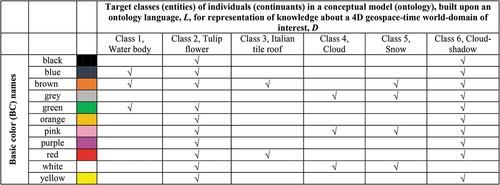
If condition m(ColorName* | c) = 0 holds for ObjectClass_c ∈ ObjectClassLegend, then posterior membership value m(c| ColorValue(x), SizeValue(x), 2DshapeValue(x), TextureValue(x), 2DspatialRelationships(x, 2Dneigh(x))) = Equation (12)(12) $\begin{array}{rl}& \mathrm{M}\mathrm{I}\mathrm{N}\left\{\begin{array}{c}\mathrm{m}\left(\mathrm{C}\mathrm{o}\mathrm{l}\mathrm{o}\mathrm{r}\mathrm{V}\mathrm{a}\mathrm{l}\mathrm{u}\mathrm{e}\left(\mathrm{x}\right)|\mathrm{c}\right),\mathrm{m}\left(\mathrm{S}\mathrm{i}\mathrm{z}\mathrm{e}\mathrm{V}\mathrm{a}\mathrm{l}\mathrm{u}\mathrm{e}\left(\mathrm{x}\right)|\mathrm{c}\right),\\ \mathrm{m}\left(2\mathrm{D}\mathrm{s}\mathrm{h}\mathrm{a}\mathrm{p}\mathrm{e}\mathrm{V}\mathrm{a}\mathrm{l}\mathrm{u}\mathrm{e}\left(\mathrm{x}\right)|\mathrm{c}\right),\mathrm{m}\left(\mathrm{T}\mathrm{e}\mathrm{x}\mathrm{t}\mathrm{u}\mathrm{r}\mathrm{e}\mathrm{V}\mathrm{a}\mathrm{l}\mathrm{u}\mathrm{e}\left(\mathrm{x}\right)|\mathrm{c}\right),\\ \mathrm{m}\left(2\mathrm{D}\mathrm{s}\mathrm{p}\mathrm{a}\mathrm{t}\mathrm{i}\mathrm{a}\mathrm{l}\mathrm{R}\mathrm{e}\mathrm{l}\mathrm{a}\mathrm{t}\mathrm{i}\mathrm{o}\mathrm{n}\mathrm{s}\mathrm{h}\mathrm{i}\mathrm{p}\mathrm{s}\left(\mathrm{x},2\mathrm{D}\mathrm{n}\mathrm{e}\mathrm{i}\mathrm{g}\mathrm{h}\left(\mathrm{x}\right)\right)|\mathrm{c}\right)\end{array}\right\}\\ & =\mathrm{M}\mathrm{I}\mathrm{N}\left\{\begin{array}{c}\sum _{\mathrm{C}\mathrm{o}\mathrm{l}\mathrm{o}\mathrm{r}\mathrm{N}\mathrm{a}\mathrm{m}{\mathrm{e}}_{\mathrm{j}},\mathrm{e}.\mathrm{g}.,\mathrm{r}\mathrm{e}\mathrm{d},\mathrm{g}\mathrm{r}\mathrm{e}\mathrm{e}\mathrm{n},\mathrm{b}\mathrm{l}\mathrm{u}\mathrm{e},\mathrm{e}\mathrm{t}\mathrm{c}.,\mathrm{w}\mathrm{i}\mathrm{t}\mathrm{h}\mathrm{j}=1}^{\mathrm{C}\mathrm{o}\mathrm{l}\mathrm{o}\mathrm{r}\mathrm{V}\mathrm{o}\mathrm{c}\mathrm{a}\mathrm{b}\mathrm{u}\mathrm{l}\mathrm{a}\mathrm{r}\mathrm{y}\mathrm{C}\mathrm{a}\mathrm{r}\mathrm{d}\mathrm{i}\mathrm{n}\mathrm{a}\mathrm{l}\mathrm{i}\mathrm{t}\mathrm{y}}\\ \mathrm{m}\left(\mathrm{C}\mathrm{o}\mathrm{l}\mathrm{o}\mathrm{r}\mathrm{V}\mathrm{a}\mathrm{l}\mathrm{u}\mathrm{e}\left(\mathrm{x}\right)|\mathrm{C}\mathrm{o}\mathrm{l}\mathrm{o}\mathrm{r}\mathrm{N}\mathrm{a}\mathrm{m}{\mathrm{e}}_{\mathrm{j}}\right)\mathrm{m}\left(\mathrm{C}\mathrm{o}\mathrm{l}\mathrm{o}\mathrm{r}\mathrm{N}\mathrm{a}\mathrm{m}{\mathrm{e}}_{\mathrm{j}}|\mathrm{c}\right),\\ \mathrm{m}\left(\mathrm{S}\mathrm{i}\mathrm{z}\mathrm{e}\mathrm{V}\mathrm{a}\mathrm{l}\mathrm{u}\mathrm{e}\left(\mathrm{x}\right)|\mathrm{c}\right),\mathrm{m}\left(2\mathrm{D}\mathrm{s}\mathrm{h}\mathrm{a}\mathrm{p}\mathrm{e}\mathrm{V}\mathrm{a}\mathrm{l}\mathrm{u}\mathrm{e}\left(\mathrm{x}\right)|\mathrm{c}\right),\\ \mathrm{m}\left(\mathrm{T}\mathrm{e}\mathrm{x}\mathrm{t}\mathrm{u}\mathrm{r}\mathrm{e}\mathrm{V}\mathrm{a}\mathrm{l}\mathrm{u}\mathrm{e}\left(\mathrm{x}\right)|\mathrm{c}\right),\\ \mathrm{m}\left(2\mathrm{D}\mathrm{s}\mathrm{p}\mathrm{a}\mathrm{t}\mathrm{i}\mathrm{a}\mathrm{l}\mathrm{R}\mathrm{e}\mathrm{l}\mathrm{a}\mathrm{t}\mathrm{i}\mathrm{o}\mathrm{n}\mathrm{s}\mathrm{h}\mathrm{i}\mathrm{p}\mathrm{s}\left(\mathrm{x},2\mathrm{D}\mathrm{n}\mathrm{e}\mathrm{i}\mathrm{g}\mathrm{h}\left(\mathrm{x}\right)\right)|\mathrm{c}\right)\end{array}\right\}\\ & =\mathrm{M}\mathrm{I}\mathrm{N}\{\mathrm{m}\left(\mathrm{C}\mathrm{o}\mathrm{l}\mathrm{o}\mathrm{r}\mathrm{N}\mathrm{a}\mathrm{m}{\mathrm{e}}^{\ast }|\mathrm{c}\right)\in \left\{0,1\right\},\mathrm{m}\left(\mathrm{S}\mathrm{i}\mathrm{z}\mathrm{e}\mathrm{V}\mathrm{a}\mathrm{l}\mathrm{u}\mathrm{e}\left(\mathrm{x}\right)|\mathrm{c}\right)\in \left[0.0,1.0\right],\\ & \mathrm{m}\left(2\mathrm{D}\mathrm{s}\mathrm{h}\mathrm{a}\mathrm{p}\mathrm{e}\mathrm{V}\mathrm{a}\mathrm{l}\mathrm{u}\mathrm{e}\left(\mathrm{x}\right)|\mathrm{c}\right)\in \left[0.0,1.0\right],\mathrm{m}\left(\mathrm{T}\mathrm{e}\mathrm{x}\mathrm{t}\mathrm{u}\mathrm{r}\mathrm{e}\mathrm{V}\mathrm{a}\mathrm{l}\mathrm{u}\mathrm{e}\left(\mathrm{x}\right)|\mathrm{c}\right)\in \left[0.0,1.0\right],\\ & \mathrm{m}\left(2\mathrm{D}\mathrm{s}\mathrm{p}\mathrm{a}\mathrm{t}\mathrm{i}\mathrm{a}\mathrm{l}\mathrm{R}\mathrm{e}\mathrm{l}\mathrm{a}\mathrm{t}\mathrm{i}\mathrm{o}\mathrm{n}\mathrm{s}\mathrm{h}\mathrm{i}\mathrm{p}\mathrm{s}\left(\mathrm{x},2\mathrm{D}\mathrm{n}\mathrm{e}\mathrm{i}\mathrm{g}\mathrm{h}\left(\mathrm{x}\right)\right)|\mathrm{c}\right)\in \left[0.0,1.0\right]\}\end{array}$(12) = 0, due to first-stage colorimetric evidence m(ColorName* | c) = 0 exclusively, irrespective of any second-stage assessment of spatial terms SizeValue(x), 2DshapeValue(x), TextureValue(x) and 2DspatialRelationships(x, 2Dneigh(x)), whose computational model is typically difficult to find and computationally expensive.

Intuitively, Equation (12)(12) $\begin{array}{rl}& \mathrm{M}\mathrm{I}\mathrm{N}\left\{\begin{array}{c}\mathrm{m}\left(\mathrm{C}\mathrm{o}\mathrm{l}\mathrm{o}\mathrm{r}\mathrm{V}\mathrm{a}\mathrm{l}\mathrm{u}\mathrm{e}\left(\mathrm{x}\right)|\mathrm{c}\right),\mathrm{m}\left(\mathrm{S}\mathrm{i}\mathrm{z}\mathrm{e}\mathrm{V}\mathrm{a}\mathrm{l}\mathrm{u}\mathrm{e}\left(\mathrm{x}\right)|\mathrm{c}\right),\\ \mathrm{m}\left(2\mathrm{D}\mathrm{s}\mathrm{h}\mathrm{a}\mathrm{p}\mathrm{e}\mathrm{V}\mathrm{a}\mathrm{l}\mathrm{u}\mathrm{e}\left(\mathrm{x}\right)|\mathrm{c}\right),\mathrm{m}\left(\mathrm{T}\mathrm{e}\mathrm{x}\mathrm{t}\mathrm{u}\mathrm{r}\mathrm{e}\mathrm{V}\mathrm{a}\mathrm{l}\mathrm{u}\mathrm{e}\left(\mathrm{x}\right)|\mathrm{c}\right),\\ \mathrm{m}\left(2\mathrm{D}\mathrm{s}\mathrm{p}\mathrm{a}\mathrm{t}\mathrm{i}\mathrm{a}\mathrm{l}\mathrm{R}\mathrm{e}\mathrm{l}\mathrm{a}\mathrm{t}\mathrm{i}\mathrm{o}\mathrm{n}\mathrm{s}\mathrm{h}\mathrm{i}\mathrm{p}\mathrm{s}\left(\mathrm{x},2\mathrm{D}\mathrm{n}\mathrm{e}\mathrm{i}\mathrm{g}\mathrm{h}\left(\mathrm{x}\right)\right)|\mathrm{c}\right)\end{array}\right\}\\ & =\mathrm{M}\mathrm{I}\mathrm{N}\left\{\begin{array}{c}\sum _{\mathrm{C}\mathrm{o}\mathrm{l}\mathrm{o}\mathrm{r}\mathrm{N}\mathrm{a}\mathrm{m}{\mathrm{e}}_{\mathrm{j}},\mathrm{e}.\mathrm{g}.,\mathrm{r}\mathrm{e}\mathrm{d},\mathrm{g}\mathrm{r}\mathrm{e}\mathrm{e}\mathrm{n},\mathrm{b}\mathrm{l}\mathrm{u}\mathrm{e},\mathrm{e}\mathrm{t}\mathrm{c}.,\mathrm{w}\mathrm{i}\mathrm{t}\mathrm{h}\mathrm{j}=1}^{\mathrm{C}\mathrm{o}\mathrm{l}\mathrm{o}\mathrm{r}\mathrm{V}\mathrm{o}\mathrm{c}\mathrm{a}\mathrm{b}\mathrm{u}\mathrm{l}\mathrm{a}\mathrm{r}\mathrm{y}\mathrm{C}\mathrm{a}\mathrm{r}\mathrm{d}\mathrm{i}\mathrm{n}\mathrm{a}\mathrm{l}\mathrm{i}\mathrm{t}\mathrm{y}}\\ \mathrm{m}\left(\mathrm{C}\mathrm{o}\mathrm{l}\mathrm{o}\mathrm{r}\mathrm{V}\mathrm{a}\mathrm{l}\mathrm{u}\mathrm{e}\left(\mathrm{x}\right)|\mathrm{C}\mathrm{o}\mathrm{l}\mathrm{o}\mathrm{r}\mathrm{N}\mathrm{a}\mathrm{m}{\mathrm{e}}_{\mathrm{j}}\right)\mathrm{m}\left(\mathrm{C}\mathrm{o}\mathrm{l}\mathrm{o}\mathrm{r}\mathrm{N}\mathrm{a}\mathrm{m}{\mathrm{e}}_{\mathrm{j}}|\mathrm{c}\right),\\ \mathrm{m}\left(\mathrm{S}\mathrm{i}\mathrm{z}\mathrm{e}\mathrm{V}\mathrm{a}\mathrm{l}\mathrm{u}\mathrm{e}\left(\mathrm{x}\right)|\mathrm{c}\right),\mathrm{m}\left(2\mathrm{D}\mathrm{s}\mathrm{h}\mathrm{a}\mathrm{p}\mathrm{e}\mathrm{V}\mathrm{a}\mathrm{l}\mathrm{u}\mathrm{e}\left(\mathrm{x}\right)|\mathrm{c}\right),\\ \mathrm{m}\left(\mathrm{T}\mathrm{e}\mathrm{x}\mathrm{t}\mathrm{u}\mathrm{r}\mathrm{e}\mathrm{V}\mathrm{a}\mathrm{l}\mathrm{u}\mathrm{e}\left(\mathrm{x}\right)|\mathrm{c}\right),\\ \mathrm{m}\left(2\mathrm{D}\mathrm{s}\mathrm{p}\mathrm{a}\mathrm{t}\mathrm{i}\mathrm{a}\mathrm{l}\mathrm{R}\mathrm{e}\mathrm{l}\mathrm{a}\mathrm{t}\mathrm{i}\mathrm{o}\mathrm{n}\mathrm{s}\mathrm{h}\mathrm{i}\mathrm{p}\mathrm{s}\left(\mathrm{x},2\mathrm{D}\mathrm{n}\mathrm{e}\mathrm{i}\mathrm{g}\mathrm{h}\left(\mathrm{x}\right)\right)|\mathrm{c}\right)\end{array}\right\}\\ & =\mathrm{M}\mathrm{I}\mathrm{N}\{\mathrm{m}\left(\mathrm{C}\mathrm{o}\mathrm{l}\mathrm{o}\mathrm{r}\mathrm{N}\mathrm{a}\mathrm{m}{\mathrm{e}}^{\ast }|\mathrm{c}\right)\in \left\{0,1\right\},\mathrm{m}\left(\mathrm{S}\mathrm{i}\mathrm{z}\mathrm{e}\mathrm{V}\mathrm{a}\mathrm{l}\mathrm{u}\mathrm{e}\left(\mathrm{x}\right)|\mathrm{c}\right)\in \left[0.0,1.0\right],\\ & \mathrm{m}\left(2\mathrm{D}\mathrm{s}\mathrm{h}\mathrm{a}\mathrm{p}\mathrm{e}\mathrm{V}\mathrm{a}\mathrm{l}\mathrm{u}\mathrm{e}\left(\mathrm{x}\right)|\mathrm{c}\right)\in \left[0.0,1.0\right],\mathrm{m}\left(\mathrm{T}\mathrm{e}\mathrm{x}\mathrm{t}\mathrm{u}\mathrm{r}\mathrm{e}\mathrm{V}\mathrm{a}\mathrm{l}\mathrm{u}\mathrm{e}\left(\mathrm{x}\right)|\mathrm{c}\right)\in \left[0.0,1.0\right],\\ & \mathrm{m}\left(2\mathrm{D}\mathrm{s}\mathrm{p}\mathrm{a}\mathrm{t}\mathrm{i}\mathrm{a}\mathrm{l}\mathrm{R}\mathrm{e}\mathrm{l}\mathrm{a}\mathrm{t}\mathrm{i}\mathrm{o}\mathrm{n}\mathrm{s}\mathrm{h}\mathrm{i}\mathrm{p}\mathrm{s}\left(\mathrm{x},2\mathrm{D}\mathrm{n}\mathrm{e}\mathrm{i}\mathrm{g}\mathrm{h}\left(\mathrm{x}\right)\right)|\mathrm{c}\right)\in \left[0.0,1.0\right]\}\end{array}$(12) shows that, in general, low-level first-stage static (non-adaptive to data)/prior knowledge-based color naming in near real-time allows, at a high-level second stage, the color name-conditional stratification of (otherwise unconditional, driven-without-prior-knowledge) multivariate 2D spatial or spectral numerical variables (either continuous or discrete, refer to Subsection 3.3.1), such as popular unconditional spectral indexes (Gao, 1996; Irish, 2000; Jordan, 1969; Kang Lee et al., 2018; Key & Benson, 1999; Liang, 2004; Lozano et al., 2007; McFeeters, 1996; Neduni & Sivakumar, 2019; Rouse et al., 1974; Roy et al., 2009; Sykas, 2020; Tucker, 1979; Xu, 2006), typically formulated as either two-band or three-band functions, see Table 3. Preliminary to high-level second-stage data analysis/interpretation, low-level first-stage data stratification, such as categorical color name-conditional estimation of numerical spatial or spectral variables in Equation (12)(12) $\begin{array}{rl}& \mathrm{M}\mathrm{I}\mathrm{N}\left\{\begin{array}{c}\mathrm{m}\left(\mathrm{C}\mathrm{o}\mathrm{l}\mathrm{o}\mathrm{r}\mathrm{V}\mathrm{a}\mathrm{l}\mathrm{u}\mathrm{e}\left(\mathrm{x}\right)|\mathrm{c}\right),\mathrm{m}\left(\mathrm{S}\mathrm{i}\mathrm{z}\mathrm{e}\mathrm{V}\mathrm{a}\mathrm{l}\mathrm{u}\mathrm{e}\left(\mathrm{x}\right)|\mathrm{c}\right),\\ \mathrm{m}\left(2\mathrm{D}\mathrm{s}\mathrm{h}\mathrm{a}\mathrm{p}\mathrm{e}\mathrm{V}\mathrm{a}\mathrm{l}\mathrm{u}\mathrm{e}\left(\mathrm{x}\right)|\mathrm{c}\right),\mathrm{m}\left(\mathrm{T}\mathrm{e}\mathrm{x}\mathrm{t}\mathrm{u}\mathrm{r}\mathrm{e}\mathrm{V}\mathrm{a}\mathrm{l}\mathrm{u}\mathrm{e}\left(\mathrm{x}\right)|\mathrm{c}\right),\\ \mathrm{m}\left(2\mathrm{D}\mathrm{s}\mathrm{p}\mathrm{a}\mathrm{t}\mathrm{i}\mathrm{a}\mathrm{l}\mathrm{R}\mathrm{e}\mathrm{l}\mathrm{a}\mathrm{t}\mathrm{i}\mathrm{o}\mathrm{n}\mathrm{s}\mathrm{h}\mathrm{i}\mathrm{p}\mathrm{s}\left(\mathrm{x},2\mathrm{D}\mathrm{n}\mathrm{e}\mathrm{i}\mathrm{g}\mathrm{h}\left(\mathrm{x}\right)\right)|\mathrm{c}\right)\end{array}\right\}\\ & =\mathrm{M}\mathrm{I}\mathrm{N}\left\{\begin{array}{c}\sum _{\mathrm{C}\mathrm{o}\mathrm{l}\mathrm{o}\mathrm{r}\mathrm{N}\mathrm{a}\mathrm{m}{\mathrm{e}}_{\mathrm{j}},\mathrm{e}.\mathrm{g}.,\mathrm{r}\mathrm{e}\mathrm{d},\mathrm{g}\mathrm{r}\mathrm{e}\mathrm{e}\mathrm{n},\mathrm{b}\mathrm{l}\mathrm{u}\mathrm{e},\mathrm{e}\mathrm{t}\mathrm{c}.,\mathrm{w}\mathrm{i}\mathrm{t}\mathrm{h}\mathrm{j}=1}^{\mathrm{C}\mathrm{o}\mathrm{l}\mathrm{o}\mathrm{r}\mathrm{V}\mathrm{o}\mathrm{c}\mathrm{a}\mathrm{b}\mathrm{u}\mathrm{l}\mathrm{a}\mathrm{r}\mathrm{y}\mathrm{C}\mathrm{a}\mathrm{r}\mathrm{d}\mathrm{i}\mathrm{n}\mathrm{a}\mathrm{l}\mathrm{i}\mathrm{t}\mathrm{y}}\\ \mathrm{m}\left(\mathrm{C}\mathrm{o}\mathrm{l}\mathrm{o}\mathrm{r}\mathrm{V}\mathrm{a}\mathrm{l}\mathrm{u}\mathrm{e}\left(\mathrm{x}\right)|\mathrm{C}\mathrm{o}\mathrm{l}\mathrm{o}\mathrm{r}\mathrm{N}\mathrm{a}\mathrm{m}{\mathrm{e}}_{\mathrm{j}}\right)\mathrm{m}\left(\mathrm{C}\mathrm{o}\mathrm{l}\mathrm{o}\mathrm{r}\mathrm{N}\mathrm{a}\mathrm{m}{\mathrm{e}}_{\mathrm{j}}|\mathrm{c}\right),\\ \mathrm{m}\left(\mathrm{S}\mathrm{i}\mathrm{z}\mathrm{e}\mathrm{V}\mathrm{a}\mathrm{l}\mathrm{u}\mathrm{e}\left(\mathrm{x}\right)|\mathrm{c}\right),\mathrm{m}\left(2\mathrm{D}\mathrm{s}\mathrm{h}\mathrm{a}\mathrm{p}\mathrm{e}\mathrm{V}\mathrm{a}\mathrm{l}\mathrm{u}\mathrm{e}\left(\mathrm{x}\right)|\mathrm{c}\right),\\ \mathrm{m}\left(\mathrm{T}\mathrm{e}\mathrm{x}\mathrm{t}\mathrm{u}\mathrm{r}\mathrm{e}\mathrm{V}\mathrm{a}\mathrm{l}\mathrm{u}\mathrm{e}\left(\mathrm{x}\right)|\mathrm{c}\right),\\ \mathrm{m}\left(2\mathrm{D}\mathrm{s}\mathrm{p}\mathrm{a}\mathrm{t}\mathrm{i}\mathrm{a}\mathrm{l}\mathrm{R}\mathrm{e}\mathrm{l}\mathrm{a}\mathrm{t}\mathrm{i}\mathrm{o}\mathrm{n}\mathrm{s}\mathrm{h}\mathrm{i}\mathrm{p}\mathrm{s}\left(\mathrm{x},2\mathrm{D}\mathrm{n}\mathrm{e}\mathrm{i}\mathrm{g}\mathrm{h}\left(\mathrm{x}\right)\right)|\mathrm{c}\right)\end{array}\right\}\\ & =\mathrm{M}\mathrm{I}\mathrm{N}\{\mathrm{m}\left(\mathrm{C}\mathrm{o}\mathrm{l}\mathrm{o}\mathrm{r}\mathrm{N}\mathrm{a}\mathrm{m}{\mathrm{e}}^{\ast }|\mathrm{c}\right)\in \left\{0,1\right\},\mathrm{m}\left(\mathrm{S}\mathrm{i}\mathrm{z}\mathrm{e}\mathrm{V}\mathrm{a}\mathrm{l}\mathrm{u}\mathrm{e}\left(\mathrm{x}\right)|\mathrm{c}\right)\in \left[0.0,1.0\right],\\ & \mathrm{m}\left(2\mathrm{D}\mathrm{s}\mathrm{h}\mathrm{a}\mathrm{p}\mathrm{e}\mathrm{V}\mathrm{a}\mathrm{l}\mathrm{u}\mathrm{e}\left(\mathrm{x}\right)|\mathrm{c}\right)\in \left[0.0,1.0\right],\mathrm{m}\left(\mathrm{T}\mathrm{e}\mathrm{x}\mathrm{t}\mathrm{u}\mathrm{r}\mathrm{e}\mathrm{V}\mathrm{a}\mathrm{l}\mathrm{u}\mathrm{e}\left(\mathrm{x}\right)|\mathrm{c}\right)\in \left[0.0,1.0\right],\\ & \mathrm{m}\left(2\mathrm{D}\mathrm{s}\mathrm{p}\mathrm{a}\mathrm{t}\mathrm{i}\mathrm{a}\mathrm{l}\mathrm{R}\mathrm{e}\mathrm{l}\mathrm{a}\mathrm{t}\mathrm{i}\mathrm{o}\mathrm{n}\mathrm{s}\mathrm{h}\mathrm{i}\mathrm{p}\mathrm{s}\left(\mathrm{x},2\mathrm{D}\mathrm{n}\mathrm{e}\mathrm{i}\mathrm{g}\mathrm{h}\left(\mathrm{x}\right)\right)|\mathrm{c}\right)\in \left[0.0,1.0\right]\}\end{array}$(12) , complies with the statistic stratification principle well known in statistics (Baraldi, 2017; Baraldi & Tiede, 2018a, 2018b; Hunt & Tyrrell, 2012) and with the popular divide-and-conquer problem solving approach (Cherkassky & Mulier, 1998), see Figure 33. In statistics, the principle of statistic stratification guarantees that “stratification will always achieve greater precision provided that the strata have been chosen so that members of the same stratum are as similar as possible in respect of the characteristic of interest” (Hunt & Tyrrell, 2012).

Table 3. Examples of scalar spectral indexes, implemented as either two-band or three-band functions, largely adopted by the remote sensing (RS) meta-science community in the feature engineering phase (Koehrsen, 2018), preliminary to (EO) optical image understanding (analysis, interpretation). Popular two-band spectral indexes are conceptually equivalent to the slope/ 1^st-order derivative/ angular coefficient of a tangent to the spectral signature in one point (Baraldi, 2017, 2019a; Baraldi et al., 2010a, 2010b, 2018a, 2018b, 2006; Baraldi & Tiede, 2018a, 2018b; Liang, 2004), see Figure 7. Each 1^st-order derivative is typically considered useful in EO optical image understanding for the detection of one specific land cover (LC) class. Hence, the name of each two-band spectral index is typically proposed as LC class-specific. Unfortunately, it is well known that infinite functions (e.g. infinite spectral signatures) can feature the same 1^st-order derivative in one point. In general, no combination of derivatives of any order can work as set of basis functions, capable of universal function approximation (Bishop, 1995; Cherkassky & Mulier, 1998). Lack of knowledge about these first principles has negative consequences on the RS common practice. First, the number and variety of scalar spectral index formulations proposed by the RS community to be considered better cross-correlated with their target LC class-specific family (envelope) of spectral signatures are ever increasing. Second, the number of scalar spectral indexes extracted from a multi-spectral (MS) signature tends to be equal or superior to the original dimensionality of the multi-spectral (MS) data space. It means that not only these scalar spectral indexes encode a lossy (irreversible) compression of a spectral signature, but their ensemble accomplishes no MS data compression at all, e.g. refer to works published in (Adamo et al., 2020; Goffi, Stroppiana, Brivio, Bordogna, & Boschetti, 2020; Kashongwe, Roy, & Bwangoy, 2020; Marconcini et al., 2020) as negative examples of MS feature engineering not to be imitated. Any increase in feature space dimensionality means increased secondary memory occupation, run-time memory occupation, computation time and cardinality of the training data set required by any machine learning (ML)-from-data algorithm to cope with the curse of data dimensionality (Bishop, 1995; Cherkassky & Mulier, 1998).

Well-known examples of two-band spectral indexes: name, acronym, range of change and reference(s)	Formulation, with wavelengths in micron and the four well-known physical model-based portions of the electromagnetic spectrum identified as: (i) visible (VIS) in (0.65-0.72), (ii) Near-Infrared (NIR) in (0.72-1.3), Middle-Infrared (MIR) in (1.3-3.0) and Thermal-Infrared (TIR) in (8.0-12.0) (Van der Meer and De Jong, 2011), see Figure 7.
Normalized Difference Vegetation Index, NDVI ∈ [−1.0, 1.0] (DLR – Deutsches Zentrum für Luft-und Raumfahrt e.V. and VEGA Technologies, 2011; ESA – European Space Agency, 2015; Jordan, 1969; Liang, 2004; Neduni & Sivakumar, 2019; Rouse et al., 1974; Sykas, 2020; Tucker, 1979)	NDVI ∈ [−1.0, 1.0] = f1(Red, NIR) = (NIR0.78÷0.90 − Red0.65÷0.68)/(Red0.65÷0.68 + NIR0.78÷0.90)
Vegetation Ratio Index (VRI), VRI ∈ [0, +∞) (Liang, 2004)	VRI ∈ [0, +∞) = f8(Red, NIR) = NIR0.78÷0.90/Red0.65÷0.68 = (1. + NDVI)/(1. – NDVI)
Aerosol-Free Vegetation Index (AFVI), AFVI ∈ [−1.0, 1.0] (Liang, 2004)	AFVI ∈ [−1.0, 1.0] = f2(NIR, MIR1) = (NIR0.78÷0.90–0.66 * MIR1.55÷1.75)/(NIR0.78÷0.90 + 0.66 * MIR1.55÷1.75)
Normalized Difference Water Index defined by McFeeters, NDWIMcFeeters ∈ [−1.0, 1.0] (Lozano, Suárez-Seoane, & de Luis, 2007; McFeeters, 1996)	NDWIMcFeeters ∈ [−1.0, 1.0] = f3(Green, NIR) = (Green0.54÷0.58 – NIR0.78÷0.90)/(Green0.54÷0.58 + NIR0.78÷0.90)
Normalized Difference Snow Index, NDSI ∈ [−1.0, 1.0] (DLR – Deutsches Zentrum für Luft-und Raumfahrt e.V. and VEGA Technologies, 2011; ESA – European Space Agency, 2015; Irish, 2000; Sykas, 2020) = Modified Normalized Difference Water Index defined by Xu, MNDWIXu ∈ [−1.0, 1.0] (Xu, 2006)	NDSI ∈ [−1.0, 1.0] = f4(Green, MIR1) = [(Green0.54÷0.58 − MIR1.57÷1.65)/(Green0.54÷0.58 + MIR1.57÷1.65)] = MNDWIXu
Normalized Difference Moisture (vice versa, drought) Index, NDMI ∈ [−1.0, 1.0] (Liang, 2004; Neduni & Sivakumar, 2019; Sykas, 2020) = Normalized Difference Water Index defined by Gao, NDWIGao (Gao, 1996)	NDMI ∈ [−1.0, 1.0] = f5(NIR, MIR1) = (NIR0.78÷0.90 − MIR1.57÷1.65)/(NIR0.78÷0.90 + MIR1.57÷1.65) = NDWIGao
Normalized Difference Bare Soil (or built-up) Index, NDBSI ∈ [−1.0, 1.0] (Kang Lee et al., 2018; Roy et al., 2009) = – NDMI	NDBSI ∈ [−1.0, 1.0] = f6(NIR, MIR1) = (MIR1.57÷1.65 − NIR0.78÷0.90)/(NIR0.78÷0.90 + MIR1.57÷1.65) = – NDMI
Normalized Difference Burned Area Index, NDBAI ∈ [−1.0, 1.0] (Key & Benson, 1999; Lozano et al., 2007; Sykas, 2020)	NDBAI ∈ [−1.0, 1.0] = f7(NIR, MIR2) = (NIR0.78÷0.90 – MIR2.08÷2.35)/(NIR0.78÷0.90 + MIR2.08÷2.35)
Three-band Greenness Index, GI ≥ 0, equal to a (downward) local concavity estimate centered on the NIR waveband (2^nd-order derivative of the spectral signature in one point) (Baraldi, 2017; Baraldi, 2019a; Baraldi et al., 2010a; Baraldi & Tiede, 2018a; Baraldi & Tiede, 2018b)	0 ≤ GI = Three-band (downward) local concavity centered on the NIR channel, augmented with sensitivity to atmospheric effects (if present, then GI tends to 0) = f9(Red, NIR, MIR1) = max{0, (NIR0.78÷0.90 / Red0.65÷0.68) + (NIR0.78÷0.90 / MIR1.57÷1.65) – (Red0.65÷0.68 / MIR1.57÷1.65)}

In addition to being eligible for higher accuracy, stratified/class-conditional data analysis, such as that pursued by Equation (12)(12) $\begin{array}{rl}& \mathrm{M}\mathrm{I}\mathrm{N}\left\{\begin{array}{c}\mathrm{m}\left(\mathrm{C}\mathrm{o}\mathrm{l}\mathrm{o}\mathrm{r}\mathrm{V}\mathrm{a}\mathrm{l}\mathrm{u}\mathrm{e}\left(\mathrm{x}\right)|\mathrm{c}\right),\mathrm{m}\left(\mathrm{S}\mathrm{i}\mathrm{z}\mathrm{e}\mathrm{V}\mathrm{a}\mathrm{l}\mathrm{u}\mathrm{e}\left(\mathrm{x}\right)|\mathrm{c}\right),\\ \mathrm{m}\left(2\mathrm{D}\mathrm{s}\mathrm{h}\mathrm{a}\mathrm{p}\mathrm{e}\mathrm{V}\mathrm{a}\mathrm{l}\mathrm{u}\mathrm{e}\left(\mathrm{x}\right)|\mathrm{c}\right),\mathrm{m}\left(\mathrm{T}\mathrm{e}\mathrm{x}\mathrm{t}\mathrm{u}\mathrm{r}\mathrm{e}\mathrm{V}\mathrm{a}\mathrm{l}\mathrm{u}\mathrm{e}\left(\mathrm{x}\right)|\mathrm{c}\right),\\ \mathrm{m}\left(2\mathrm{D}\mathrm{s}\mathrm{p}\mathrm{a}\mathrm{t}\mathrm{i}\mathrm{a}\mathrm{l}\mathrm{R}\mathrm{e}\mathrm{l}\mathrm{a}\mathrm{t}\mathrm{i}\mathrm{o}\mathrm{n}\mathrm{s}\mathrm{h}\mathrm{i}\mathrm{p}\mathrm{s}\left(\mathrm{x},2\mathrm{D}\mathrm{n}\mathrm{e}\mathrm{i}\mathrm{g}\mathrm{h}\left(\mathrm{x}\right)\right)|\mathrm{c}\right)\end{array}\right\}\\ & =\mathrm{M}\mathrm{I}\mathrm{N}\left\{\begin{array}{c}\sum _{\mathrm{C}\mathrm{o}\mathrm{l}\mathrm{o}\mathrm{r}\mathrm{N}\mathrm{a}\mathrm{m}{\mathrm{e}}_{\mathrm{j}},\mathrm{e}.\mathrm{g}.,\mathrm{r}\mathrm{e}\mathrm{d},\mathrm{g}\mathrm{r}\mathrm{e}\mathrm{e}\mathrm{n},\mathrm{b}\mathrm{l}\mathrm{u}\mathrm{e},\mathrm{e}\mathrm{t}\mathrm{c}.,\mathrm{w}\mathrm{i}\mathrm{t}\mathrm{h}\mathrm{j}=1}^{\mathrm{C}\mathrm{o}\mathrm{l}\mathrm{o}\mathrm{r}\mathrm{V}\mathrm{o}\mathrm{c}\mathrm{a}\mathrm{b}\mathrm{u}\mathrm{l}\mathrm{a}\mathrm{r}\mathrm{y}\mathrm{C}\mathrm{a}\mathrm{r}\mathrm{d}\mathrm{i}\mathrm{n}\mathrm{a}\mathrm{l}\mathrm{i}\mathrm{t}\mathrm{y}}\\ \mathrm{m}\left(\mathrm{C}\mathrm{o}\mathrm{l}\mathrm{o}\mathrm{r}\mathrm{V}\mathrm{a}\mathrm{l}\mathrm{u}\mathrm{e}\left(\mathrm{x}\right)|\mathrm{C}\mathrm{o}\mathrm{l}\mathrm{o}\mathrm{r}\mathrm{N}\mathrm{a}\mathrm{m}{\mathrm{e}}_{\mathrm{j}}\right)\mathrm{m}\left(\mathrm{C}\mathrm{o}\mathrm{l}\mathrm{o}\mathrm{r}\mathrm{N}\mathrm{a}\mathrm{m}{\mathrm{e}}_{\mathrm{j}}|\mathrm{c}\right),\\ \mathrm{m}\left(\mathrm{S}\mathrm{i}\mathrm{z}\mathrm{e}\mathrm{V}\mathrm{a}\mathrm{l}\mathrm{u}\mathrm{e}\left(\mathrm{x}\right)|\mathrm{c}\right),\mathrm{m}\left(2\mathrm{D}\mathrm{s}\mathrm{h}\mathrm{a}\mathrm{p}\mathrm{e}\mathrm{V}\mathrm{a}\mathrm{l}\mathrm{u}\mathrm{e}\left(\mathrm{x}\right)|\mathrm{c}\right),\\ \mathrm{m}\left(\mathrm{T}\mathrm{e}\mathrm{x}\mathrm{t}\mathrm{u}\mathrm{r}\mathrm{e}\mathrm{V}\mathrm{a}\mathrm{l}\mathrm{u}\mathrm{e}\left(\mathrm{x}\right)|\mathrm{c}\right),\\ \mathrm{m}\left(2\mathrm{D}\mathrm{s}\mathrm{p}\mathrm{a}\mathrm{t}\mathrm{i}\mathrm{a}\mathrm{l}\mathrm{R}\mathrm{e}\mathrm{l}\mathrm{a}\mathrm{t}\mathrm{i}\mathrm{o}\mathrm{n}\mathrm{s}\mathrm{h}\mathrm{i}\mathrm{p}\mathrm{s}\left(\mathrm{x},2\mathrm{D}\mathrm{n}\mathrm{e}\mathrm{i}\mathrm{g}\mathrm{h}\left(\mathrm{x}\right)\right)|\mathrm{c}\right)\end{array}\right\}\\ & =\mathrm{M}\mathrm{I}\mathrm{N}\{\mathrm{m}\left(\mathrm{C}\mathrm{o}\mathrm{l}\mathrm{o}\mathrm{r}\mathrm{N}\mathrm{a}\mathrm{m}{\mathrm{e}}^{\ast }|\mathrm{c}\right)\in \left\{0,1\right\},\mathrm{m}\left(\mathrm{S}\mathrm{i}\mathrm{z}\mathrm{e}\mathrm{V}\mathrm{a}\mathrm{l}\mathrm{u}\mathrm{e}\left(\mathrm{x}\right)|\mathrm{c}\right)\in \left[0.0,1.0\right],\\ & \mathrm{m}\left(2\mathrm{D}\mathrm{s}\mathrm{h}\mathrm{a}\mathrm{p}\mathrm{e}\mathrm{V}\mathrm{a}\mathrm{l}\mathrm{u}\mathrm{e}\left(\mathrm{x}\right)|\mathrm{c}\right)\in \left[0.0,1.0\right],\mathrm{m}\left(\mathrm{T}\mathrm{e}\mathrm{x}\mathrm{t}\mathrm{u}\mathrm{r}\mathrm{e}\mathrm{V}\mathrm{a}\mathrm{l}\mathrm{u}\mathrm{e}\left(\mathrm{x}\right)|\mathrm{c}\right)\in \left[0.0,1.0\right],\\ & \mathrm{m}\left(2\mathrm{D}\mathrm{s}\mathrm{p}\mathrm{a}\mathrm{t}\mathrm{i}\mathrm{a}\mathrm{l}\mathrm{R}\mathrm{e}\mathrm{l}\mathrm{a}\mathrm{t}\mathrm{i}\mathrm{o}\mathrm{n}\mathrm{s}\mathrm{h}\mathrm{i}\mathrm{p}\mathrm{s}\left(\mathrm{x},2\mathrm{D}\mathrm{n}\mathrm{e}\mathrm{i}\mathrm{g}\mathrm{h}\left(\mathrm{x}\right)\right)|\mathrm{c}\right)\in \left[0.0,1.0\right]\}\end{array}$(12) , is typically computationally more efficient than unconditional/driven-without-prior-knowledge data analysis, such as unconditional spatial or spectral feature extraction (see Table 3), where one spatial or spectral feature operator is applied image-wide on an unconditional basis, i.e. without a focus-of-visual-attention mechanism equivalent to a data masking/stratification criterion (Baraldi, 2017; Matsuyama & Hwang, 1990). For example, the computational complexity of first-stage deductive/ top-down/ prior knowledge-based color naming, capable of numerical color image stratification into static (non-adaptive to data) categorical color names/ strata/ layers, is linear with image size (refer to this Subsection above), i.e. static (non-adaptive to data) color naming is near real-time, whereas 2D spatial features, e.g. 2D shape indexes (Baraldi, 2017; Baraldi & Soares, 2017), whose computational complexity is typically polynomial, are expensive to compute in the (2D) image-plane.

Figure 33. Phenological transitions in time: traditional driven-without-knowledge versus innovative driven-by-knowledge (stratified, masked, class-conditional) inductive data learning approach to either pixel-based or image object-based vegetation/not-vegetation classification through time, in a time series of, for example, 8-band WorldView-2 multi-spectral (MS) images. Traditional approach (Huth et al., 2012): Step (1) = Driven-without-knowledge vegetation spectral index extraction (see Figure 7) through time, either pixel-based or image object-based. In more detail, the well-known two-band Normalized Difference Vegetation Index (NDVI) (Jordan, 1969; Liang, 2004; Neduni & Sivakumar, 2019; Rouse et al., 1974; Sykas, 2020; Tucker, 1979) is employed, where NDVI ∈ [−1.0, 1.0] = f₁(Red, NIR) = (NIR_0.78÷0.90 – Red_0.65÷0.68)/(NIR_0.78÷0.90 + Red_0.65÷0.68), which is monotonically increasing with the dimensionless Vegetation Ratio Index (VRI), where VRI ∈ (0, +∞) = NIR_0.78÷0.90 / Red_0.65÷0.68 = (1. + NDVI)/(1. – NDVI) (Liang, 2002), see Table 3. Hence, NDVI = f₁(R, NIR) is conceptually equivalent to the angular coefficient (1^st-order derivative) of a tangent to the spectral signature in one point (Baraldi, 2017, 2019a; Baraldi et al., 2010a, 2010b, 2018a, 2018b, 2006; Baraldi & Tiede, 2018a, 2018b; Liang, 2004). Step (2) = Pixel- or object-based supervised NDVI data classification, equivalent to posterior probability p(c = Vegetation class | NDVI = f₁(R, NIR)), e.g. C5.0 supervised data learning decision tree classification (Huth et al., 2012). As viable alternative to the aforementioned step (1), for vegetation detection purposes, the traditional univariate two-band NDVI analysis through time is replaced by a more informative and more efficient class-conditional multi-variate data analysis of all spectral channels through time. In practice, automatic linear-time estimation of a class-conditional scalar greenness index (GI), p(GI = f₉(R, NIR, MIR1) | Vegetation class = g(h(All Bands))), can be applied through time for within-vegetation class discrimination, based on: (i) a three-band scalar greenness index, GI, equivalent to a (downward) concavity (2^nd-order derivative) centered on the NIR waveband = f₉(R, NIR, MIR1) ∈ [0,∞) = max {0, (NIR/R) + (NIR/MIR_1.55÷1.75) − (R/MIR_1.55÷1.75)} ≥ 0 (Baraldi et al., 2010a) (see Table 3), (ii) a Vegetation class, estimated (with approximation) by a logical-AND/OR combination of Satellite Image Automatic Mapper (SIAM)’s color names (see Figure 32), where each SIAM color name = h(All Bands) (Baraldi, 2017, 2019a; Baraldi et al., 2010a, 2010b, 2018a, 2018b, 2006; Baraldi & Tiede, 2018a, 2018b) (see Figure 30), hence, Vegetation class ≈ g(color names) = g(h(All Bands)), see Figure 32.

To better understand the potential impact of a low-level ‘CV ⊃ EO-IU ⊃ ARD’ stage capable of deductive color naming in near real-time upon the RS common practice adopted by large portions of the RS meta-science community involved with Equation (3)(3) $\text{lsquo}\mathrm{A}\mathrm{R}\mathrm{D}\subset \mathrm{E}\mathrm{O}-\mathrm{I}\mathrm{U}\subset \mathrm{C}\mathrm{V}\subset \mathrm{A}\mathrm{G}\mathrm{I}\subset \mathrm{C}\mathrm{o}\mathrm{g}\mathrm{n}\mathrm{i}\mathrm{t}\mathrm{i}\mathrm{v}\mathrm{e}\mathrm{s}\mathrm{c}\mathrm{i}\mathrm{e}\mathrm{n}\mathrm{c}\mathrm{e}\text{rsquo}$(3) = ‘ARD ⊂ EO-IU ⊂ CV ⊂ AGI ⊂ Cognitive science’ problems, let us briefly investigate potential gains in accuracy and efficiency stemming from stratified/ masked/ class-conditional/ Bayesian/ driven-by-prior-knowledge extraction of popular scalar spectral indexes (see Figure 33), in comparison with traditional image-wide unconditional/driven-without-prior-knowledge extraction of two- or three-band scalar spectral indexes, see Table 3.

In the MS/ SS/ HS feature engineering first phase (Koehrsen, 2018) (refer to Subsection 3.1), preliminary to EO optical image understanding (interpretation, classification) second stage, a standard practice of the RS meta-science community is image-wide extraction of unconditional/driven-without-prior-knowledge scalar spectral indexes (Adamo et al., 2020; DLR – Deutsches Zentrum für Luft-und Raumfahrt e.V. and VEGA Technologies, 2011; ESA – European Space Agency, 2015; Gao, 1996; Goffi et al., 2020; Huth et al., 2012; Jordan, 1969; Kang Lee et al., 2018; Kashongwe et al., 2020; Key & Benson, 1999; Liang, 2004; Lozano et al., 2007; Marconcini et al., 2020; McFeeters, 1996; Neduni & Sivakumar, 2019; Rouse et al., 1974; Roy et al., 2009; Sykas, 2020; Tucker, 1979; Xu, 2006). Typically formulated as either two-band or three-band functions (see Table 3), scalar spectral index formulations have been ever increasing in popularity and variety (refer to references listed in this Subsection above), since the launch of the NASA Landsat-1 satellite in 1972 (refer to Section 2).

To explain why the variety of unconditional/driven-without-prior-knowledge two-band and three-band scalar spectral indexes presented in the RS literature and extracted in the RS feature engineering phase is ever increasing (see Table 3), let us observe that, for spectral signature (pattern) recognition/classification purposes (see Figure 7, Figure 30 and Figure 33), chlorophyll absorption phenomena in photosynthetically active vegetation are typically investigated (intercepted, modeled) by so-called vegetation spectral indexes, such as the well-known two-band Normalized Difference Vegetation Index (NDVI), where NDVI ∈ [−1.0, 1.0] = f₁(Red, NIR) = f₁(Red_0.65÷0.68, NIR_0.78÷0.90) = (NIR_0.78÷0.90 – Red_0.65÷0.68) / (NIR_0.78÷0.90 + Red_0.65÷0.68) (Jordan, 1969; Liang, 2004; Neduni & Sivakumar, 2019; Rouse et al., 1974; Sykas, 2020; Tucker, 1979). The popular NDVI is monotonically increasing with the dimensionless Vegetation Ratio Index (VRI), where VRI ∈ [0, +∞) = f₈(Red, NIR) = f₈(Red_0.65÷0.68, NIR_0.78÷0.90) = NIR_0.78÷0.90 / Red_0.65÷0.68 = (1. + NDVI)/(1. – NDVI) (Liang, 2004). Interdependent scalar spectral indexes NDVI and VRI are intuitive to understand and easy to implement, they are somehow robust to changes in solar illumination, atmospheric conditions and sensor viewing geometry affecting surface reflectance, but are affected by well-known limitations (Liang, 2004). NDVI is highly correlated with (and therefore can be effective in predicting) biophysical variables about vegetation structure and the state of the vegetation cover, such as leaf density and distribution leaf water content, age, mineral deficiencies, parasitic attacks, etc., when canopy is not too dense or too sparse. If the canopy is too dense, NDVI saturates. If a canopy is too sparse, background signal (e.g. soil) can change NDVI significantly, due to mixed-pixel effects. VRI is much slower to saturate than NDVI when a canopy is very dense, but it is not more robust than NDVI to changes in soil reflectance underneath the canopy. To increase robustness of NDVI and VRI to changes in canopy surface reflectance due to disturbing factors including the effects of background soils, many alternative so-called vegetation spectral indexes have been proposed, such as the Aerosol-Free Vegetation Index (AFVI) (Liang, 2004), formulated as AFVI ∈ [−1.0, 1.0] = f₂(NIR, MIR1) = f₂(NIR_0.78÷0.90, MIR_1.55÷1.75) = (NIR_0.78÷0.90 – 0.66 * MIR_1.55÷1.75) / (NIR_0.78÷0.90 + 0.66 * MIR_1.55÷1.75), see Table 3. Water content absorption phenomena in photosynthetically active vegetation (see Figure 7 and Figure 30) are traditionally intercepted by so-called moisture or, vice versa, drought spectral indexes (Poussin et al., 2021), such as the two-band Normalized Difference Moisture Index (NDMI) (Liang, 2004; Neduni & Sivakumar, 2019; Sykas, 2020), also known as the Normalized Difference Water Index defined by Gao (NDWI_Gao) (Gao, 1996), where NDMI ∈ [−1.0, 1.0] = NDWI_Gao = f₅(NIR, MIR1) = f₅(NIR_0.78÷0.90, MIR_1.55÷1.75) = (NIR_0.78÷0.90 – MIR_1.55–1.75) / (NIR_0.78÷0.90 + MIR_1.55÷1.75), which is inversely related to the so-called Normalized Difference Bare Soil Index (NDBSI), proposed in (Kang Lee et al., 2018; Roy et al., 2009), where NDBSI ∈ [−1.0, 1.0] = – NDMI = – NDWI_Gao = (MIR_1.55÷1.75 – NIR_0.78÷0.90) / (MIR_1.55÷1.75 + NIR_0.78÷0.90), see Table 3. Alternative to indexes NDWI_Gao(NIR_0.78÷0.90, MIR_1.55÷1.75) = NDMI = – NDBSI, several so-called water spectral indexes have been proposed in the RS literature, such as the NDWI defined by McFeeters (Lozano et al., 2007; McFeeters, 1996), where NDWI_McFeeters ∈ [−1.0, 1.0] = f₃(Green, NIR) = f₃(Green_0.54÷0.58, NIR_0.78÷0.90) = (Green_0.54÷0.58 – NIR_0.78÷0.90) / (Green_0.54÷0.58+ NIR_0.78÷0.90) and the Modified Normalized Difference Water Index defined by Xu (MNDWI_Xu) (Xu, 2006), better known as Normalized Difference Snow Index (NDSI) (DLR – Deutsches Zentrum für Luft-und Raumfahrt e.V. and VEGA Technologies, 2011; ESA – European Space Agency, 2015; Irish, 2000; Sykas, 2020), where MNDWI_Xu ∈ [−1.0, 1.0] = NDSI = f₄(Green, MIR1) = f₄(Green_0.54÷0.58, MIR_1.57÷1.65) = (Green_0.54÷0.58 – MIR_1.57÷1.65) / (Green_0.54÷0.58 + MIR_1.57÷1.65), see Table 3.

Worth noting, according to commonsense knowledge (refer to Section 2) based on human visul perception (see Figure 20), which is sensitive to the visible portion of the electromagnetic spectrum exclusively (see Figure 7 and Figure 30), spectral signatures of LC classes Water and Snow are very different and easy to be discriminated. This perceptual observation (true-fact) is quantitatively supported by the RS literature, where spectral signatures of LC classes Water and Snow are known to be very different, both locally and globally, across the electromagnetic spectrum, ranging from visible to thermal wavelengths, see Figure 7 and Figure 30 (Swain & Davis, 1978). In spite of well-known local and global differences in the intensity and shape information components of the spectral signatures of LC classes Water and Snow, the formulation of the two-band scalar spectral index MNDWI_Xu(Green_0.54÷0.58, MIR_1.55–1.75), semantically associated by name with LC Water, is the same as that of NDSI(Green_0.54÷0.58, MIR_1.55–1.75), semantically linked by name with LC Snow.

This short review of two-band scalar spectral indexes widely adopted in the RS community reveals that, in spectral index naming, the RS community typically calls the same subsymbolic (numerical) two-band spectral index formulation by different names pointing at different symbolic LC classes (where LC classes are discrete and semantic entities in a totally exhaustive and mutually exclusive LC class taxonomy, which is part-of a 7D conceptual world model available a priori, in addition to sensory data, refer to Section 2). It means that, in agreement with commonsense knowledge (refer to Section 2), subsymbolic numerical spectral indexes/ features/ properties “cannot always be inverted to unique [symbolic] LC class names”, just like discrete spectral end-members typically adopted in hyper-spectral image interpretation “cannot always be inverted to unique LC class names” (Adams et al., 1995).

An obvious conjecture stemming from this observation (true-fact) is that the number and variety of scalar spectral indexes are ever-increasing in the RS literature and common practice because values (instantiations) of subsymbolic numerical spectral indexes are typically inverted to/ associated with/ misunderstood (confused) with symbolic (discrete and semantic) entities/LC classes. The consequence of being misunderstood because erroneously thought as one-to-one related with meaning/semantics is that numerical spectral indexes are typically misused by the RS community involved with the feature engineering first stage, preliminary to second-stage feature/pattern recognition and interpretation in inherently ill-posed ‘CV ⊃ EO-IU ⊃ ARD’ problems.

To prove this conjecture in the promotion of a RS better practice, where scalar spectral indexes must be better understood as precondition for better use, the (true, unequivocal) mathematical meaning of unconditional/driven-without-prior-knowledge two-band and three-band scalar spectral indexes is highlighted below.

Popular two-band scalar spectral indexes (see Table 3) are conceptually equivalent to the 1^st-order derivative/ angular coefficient/ slope of a tangent to the spectral signature in one point (Baraldi, 2017, 2019a; Baraldi et al., 2010a, 2010b, 2018a, 2018b, 2006; Baraldi & Tiede, 2018a, 2018b; Liang, 2004), see Figure 7 and Figure 30. It is well known that infinite functions can feature the same 1^st-order derivative in one point. Since two-band scalar spectral indexes (see Table 3) are conceptually equivalent to the 1^st-order derivative/ angular coefficient/ slope of a tangent to the spectral signature in one point, then, in general, they should never be inverted to unique LC class names.

As a typical example of (mis)use of two-band scalar spectral indexes by the relevant portion of the RS community involved with ‘CV ⊃ EO-IU ⊃ ARD’ tasks, let us consider the popular ESA Sentinel 2 imaging sensor-specific Level 2 Sen2Cor software toolbox, developed and run by ESA or distributed by ESA free-of-cost to be run on the user side (DLR – Deutsches Zentrum für Luft-und Raumfahrt e.V. and VEGA Technologies, 2011; ESA – European Space Agency, 2015). The ESA Sen2Cor software delivers as output a stack of two co-products (refer to Section 2): first, a subsymbolic 12-band Sentinel-2 MSI image co-product radiometrically calibrated into SURF 3-of-3 values, (supposedly) corrected from atmospheric, adjacency and topographic effects (refer to Subsection 3.3.2), stacked (overlapped) with, second, a symbolic SCM co-product, whose thematic map legend includes quality layers Cloud and Cloud-shadow (also refer to Figure 38 below in this text). The ESA Sen2Cor’s SCM co-product is generated by a pixel-based (2D spatial context-insensitive) static (non-adaptive to data) decision tree for MS color naming, erroneously considered a LC class classifier. Actually, a binary relationship between color names and LC classes does exist, i.e. color names are merely attributes of LC classes and the former should never be confused with the latter as one-to-one related sets, see Figure 32. The ESA Sen2Cor’s pixel-based decision tree classifier of numerical color values into a discrete and finite vocabulary of color names pursues crisp (hard) thresholding/partitioning of one pair of popular two-band scalar spectral indexes (see Table 3), specifically, the aforementioned NDVI ∈ [−1.0, 1.0] = f₁(Red, NIR) = (NIR_0.78÷0.90 – Red_0.65÷0.68) / (NIR_0.78÷0.90 + Red_0.65÷0.68) and the so-called NDSI ∈ [−1.0, 1.0] = f₄(Green, MIR1) = (Green_0.54÷0.58 – MIR_1.55÷1.75) / (Green_0.54÷0.58 + MIR_1.55÷1.75) = MNDWI_Xu (Irish, 2000; Sykas, 2020; Xu, 2006), where the latter is considered useful by ESA for the detection of LC class Snow (DLR – Deutsches Zentrum für Luft-und Raumfahrt e.V. and VEGA Technologies, 2011; ESA – European Space Agency, 2015), rather than for the discrimination of LC class Water in comparison with LC class Built-up land (whose spectral response in the MIR band tends to be ≥ than the response in visible Green, unlike that of LC class Water), as claimed by Xu (Xu, 2006), see Table 3. This is tantamount to saying that, first, the Sen2Cor’s MS feature engineering first phase (Koehrsen, 2018), preliminary to second-stage MS data interpretation for SCM generation, pursues the lossy (irreversible) compression of a 12-band MS signature onto a 2D measurement space, consisting of two angular coefficients of a tangent pair to the MS signature in two points. Since, in general, infinite functions can feature the same 1^st-order derivative in one point then the Sen2Cor’s feature engineering first stage is affected by the irreversible loss (lossy compression) onto a 2D feature space of both the 12-band MS shape and MS intensity information components of a Sentinel-2 imaging sensor-specific 12-band MS signature, see Figure 7 and Figure 30. Second, the Sen2Cor’s decision-tree second stage maps a (lossy) compressed 2D feature space, consisting of a pair of two-band scalar spectral indexes, into a discrete and finite categorical/nominal vocabulary of MS color names/hyperpolyhedra, where MS color names/hyperpolyhedra provide a mutually exclusive and totally exhaustive hyperpolyhedralization of the input 2D color-derived measurement space, see Figure 29. In the Sen2Cor’s decision-tree mapping function of a 2D color-related value into one color name belonging to a finite and discrete vocabulary of color names, the output color name should never be confused with any LC class/entity featuring that color name as attribute, see Figure 32.

Whereas popular two-band spectral indexes are conceptually equivalent to the angular coefficient/ slope/ 1^st-order derivative of a tangent to the spectral signature in one point, three-band spectral indexes are conceptually equivalent to a 2^nd-order derivative as local measure of concavity of the spectral signature centered on one point (Liang, 2004). For example, in (Baraldi, 2017, 2019a; Baraldi et al., 2010a, 2010b, 2018a, 2018b, 2006; Baraldi & Tiede, 2018a, 2018b), an original three-band Greenness Index (GI) is formulated as a (downward) local concavity estimate of photosynthetically active vegetation, centered on the NIR waveband (2^nd-order derivative of the spectral signature in one point),

0 ≤ GI = GI(Red, NIR, MIR1) = Three-band (downward) local concavity centered on the NIR channel, augmented with sensitivity to atmospheric effects (if present, then GI tends to 0) = f₉(Red, NIR, MIR1) = f₉(Red_0.65÷0.68, NIR_0.78÷0.90, MIR_1.57÷1.65) = max{0, (NIR_0.78÷0.90 / Red_0.65÷0.68) + (NIR_0.78÷0.90 / MIR_1.57÷1.65) – (Red_0.65÷0.68 / MIR_1.57÷1.65)},

see Table 3 and Figure 33 (for more details about the rationale of this three-band scalar spectral index, GI(Red, NIR, MIR1), refer to this Subsection below).

According to the field of continuous function approximation at the basis of ML-from-data for either function regression or classification tasks (Bishop, 1995; Cherkassky & Mulier, 1998), a wide, but finite set of approximating functions belonging to the same class of functions can work as universal approximator, typically equivalent to a linear combination of basis functions (Cherkassky & Mulier, 1998). For example, according to the well-known Weierstrass theorem, any continuous function on a compact set can be uniformly approximated by a polynomial (Cherkassky & Mulier, 1998), i.e. for any function f(x) and any any positive approximation error ε > 0, there exists an algebraic polynomial of degree m, $p_m\left(x\right)=\sum _{i=0}^m{w}_i{x}^i$, such that || f(x) – p_m(x)|| < ε, for every x.

Unfortunately, no combination of function derivatives of any order can work as set of basis functions, capable of universal function approximation (Bishop, 1995; Cherkassky & Mulier, 1998). It means that if, in the fundamental feature engineering first phase (Koehrsen, 2018), preliminary to second-stage EO optical image interpretation (classification, analysis), any two- or three-band spectral index extraction occurs (see Table 3), then it always causes an irreversible loss in (lossy compression of) the multivariate shape and multivariate intensity information components of a spectral signature (Baraldi, 2017, 2019a; Baraldi et al., 2010a, 2010b, 2018a, 2018b, 2006; Baraldi & Tiede, 2018a, 2018b), see Figure 30.

Lack of knowledge about these first principles has negative consequences on the RS common practice. First, the number and variety of scalar spectral index formulations proposed by the RS community to be considered better cross-correlated with their target LC class-specific family (envelope) of spectral signatures are ever increasing. Second, the number of scalar spectral indexes extracted from a MS signature tends to be equal or superior to the original dimensionality of the MS data space. It means that not only these scalar spectral indexes encode a lossy (irreversible) compression of a MS signature, but their ensemble accomplishes no MS data compression at all, e.g. refer to works published in (Adamo et al., 2020; Goffi et al., 2020; Kashongwe et al., 2020; Marconcini et al., 2020) as negative examples of a MS feature engineering phase not to be imitated because affected by lossy data transformation together with augmented data dimensionality. Any increase in feature space dimensionality means increased secondary memory occupation, run-time memory occupation, computation time and cardinality of the training data set required by any ML-from-data algorithm to cope with the curse of data dimensionality (Bishop, 1995; Cherkassky & Mulier, 1998) (refer to Subsection 3.1).

As another example of bad practice typically affecting the wide portion of the RS community involved with ‘CV ⊃ EO-IU ⊃ ARD’ tasks, let us consider a traditional 1D approach to MS image time-series interpretation for vegetation/not-vegetation detection through time, either pixel-based or image object-based (see Figure 22), widely adopted by the RS community to investigate phenological transitions (Huth et al., 2012), see the top workflow in Figure 33. In (Huth et al., 2012), first, an unconditional NDVI = f₁(Red_0.65÷0.68, NIR_0.78÷0.90) operator is applied image-wide through the MS image time series. Next, a time series of scalar NDVI values, either pixel-based or image object-based, is input to a second-stage vector data classifier, e.g. a C5.0 adaptive learning-from-data decision tree classifier (Huth et al., 2012). It means that, in (Huth et al., 2012), any spectral signature of the Earth surface, sampled by an 8-channel WorldView-2 MS imaging sensor, is encoded by an irreversible (lossy) compression method into a 1D two-band scalar spectral index, conceptually equivalent to the ratio of two spectral bands selected from the available eight spectral channels, whereas the six remaining channels of the MS information are totally ignored for LC class Vegetation detection through time, see Figure 7, Figure 30 and Figure 33.

In agreement with the principle of statistic stratification well known in statistics (Hunt & Tyrrell, 2012), the lower workflow shown in Figure 33 provides an alternative, more informative and computationally more efficient approach to LC class Vegetation-through-time classification, capable of stratified/ class-conditional/ Bayesian multi-variate data analysis of all spectral channels through time. In practice, an automatic linear-time LC Vegetation class-conditional three-band scalar greenness index (see Table 3)

0 ≤ GI _{Vegetation LC class-conditional}(All Bands) = p(GI = f₉(R, NIR, MIR1) | LC class Vegetation ≈ g(h(All Bands))),

can be applied through time for within-Vegetation class discrimination by a second-stage vector data classifier (see Figure 33), based on:

1. A single-date LC class Vegetation detection, where LC class Vegetation is estimated, with approximation, single-date (for each individual image in the image time-series) as a logical AND/OR combination of SIAM color names, where each SIAM color name = h(All Bands) (Baraldi, 2017, 2019a; Baraldi et al., 2010a, 2010b, 2018a, 2018b, 2006; Baraldi & Tiede, 2018a, 2018b) (see Figure 30), hence, LC class Vegetation ≈ g(color names) = g(h(All Bands)), see Figure 32.

2. A single-date driven-without-prior-knowledge three-band scalar greenness index, GI = f₉(R, NIR, MIR1) = f₉(Red_0.65÷0.68, NIR_0.78÷0.90, MIR_1.57÷1.65) (see Table 3), formulated as follows.

   (Downward) concavity (2^nd-order derivative) centered on the NIR waveband = 

   Three-band Greenness Index(Red_0.65÷0.68, NIR_0.78÷0.90, MIR_1.55÷1.75), augmented with sensitivity to atmospheric effects (if present, then GI tends to 0) = GI(Red_0.65÷0.68, NIR_0.78÷0.90, MIR_1.55÷1.75) ∈ [0,∞) = max {0, (NIR/R) + (NIR/MIR1) − (R/MIR1)} ≥ 0,

   to be estimated exclusively within the LC Vegetation layer (stratum, mask, class) detected single date. It becomes a driven-by-prior-knowledge downward concavity, GI_{Vegetation LC class-conditional}(All Bands) = p(GI = f₉(R, NIR, MIR1) | LC class Vegetation ≈ g(h(All Bands))).

3. The two previous steps for single-date estimation of a driven-by-prior-knowledge downward concavity, GI_{Vegetation LC class-conditional}(All Bands), are repeated across the MS image time-series, preliminary to high-level second-stage EO image time-series classification.

About the aforementioned three-band GI formulation, with GI(Red_0.65÷0.68, NIR_0.78÷0.90, MIR_1.55÷1.75) ∈ [0, ∞) = (Downward) concavity (2^nd-order derivative) centered on the NIR waveband = max{0, (NIR/R) + (NIR/MIR) – (R/MIR)} ≥ 0, let us consider that, in agreement with a convergence-of-evidence approach to MS signature parameterization for ‘CV ⊃ EO-IU ⊃ ARD’ purposes (see Figure 7 and Figure 30):

• The first term is the so-called vegetation ratio index, VRI ∈ [0, +∞) = NIR_0.78÷0.90 / Red_0.65÷0.68 = (1. + NDVI) / (1. – NDVI), see Table 3. In addition to NDVI, VRI is related to the greenness second linear function in the Tasseled Cap transformation of data generated from the Landsat-5 TM or Landsat-7 Enhanced TM+ (Liang, 2004, p. 260) and linearly cross-correlated with chlorophyll absorption phenomena in reflectance values of “green (photosynthetically active) vegetation” (Liang, 2004; Swain & Davis, 1978), see Figure 7 and Figure 30.

• The second term, (NIR_0.78÷0.90 / MIR_1.55÷1.75) ≥ 0, is linearly cross-correlated with water absorption phenomena in reflectance values of “green (photosynthetically active) vegetation” (Liang, 2004; Swain & Davis, 1978), see Figure 7 and Figure 30. In fact, this second term is directly related to the aforementioned two-band “moisture-related” spectral indexes NDMI = NDWI_Gao = (NIR_0.78÷0.90 – MIR_1.55÷1.75) / (NIR_0.78÷0.90 + MIR_1.55÷1.75) = – NDBSI ∈ [−1.0, 1.0], see Table 3. In more detail, (NIR_0.78÷0.90 / MIR_1.55÷1.75) = (1. + NDMI)/(1. – NDMI) ≥ 0. It is also positively correlated with AFVI ∈ [−1.0, 1.0] = (NIR_0.78÷0.90–0.66 * MIR_1.55÷1.75)/(NIR_0.78÷0.90 + 0.66 * MIR_1.55÷1.75), see Table 3. In agreement with natural language and intuition, when a two-band spectral index NDBSI, correlated with LC class Bare soil, increases, then the proposed three-band GI, correlated with LC class Vegetation, decreases and vice versa.

• The third term, (−1) * (Red_0.65÷0.68 / MIR_1.55÷1.75), is directly related to the so-called wetness tasseled cap component (Liang, 2004, p. 260). It is subtracted from the previous two terms to model correlation of spectral reflectance values with non-target phenomena, such as atmospheric effects and LC class Snow, whose presence means that no target phenomenon of “green (photosynthetically active) vegetation” can be detected with high confidence (Liang, 2004; Swain & Davis, 1978). This third term is highly correlated, in terms of negative PLCC values (Kreyszig, 1979; Sheskin, 2000; Tabachnick & Fidell, 2014) estimated image-wide (see Figure 9), with the two aforementioned two-band spectral indexes NDSI = MNDWI_Xu ∈ [−1.0, 1.0] = (Green_0.54÷0.58– MIR_1.55÷1.75) / (Green_0.54÷0.58 + MIR_1.55÷1.75) (see Table 3), considered useful for, respectively, the detection of LC class Snow (DLR – Deutsches Zentrum für Luft-und Raumfahrt e.V. and VEGA Technologies, 2011; ESA – European Space Agency, 2015; Irish, 2000; Sykas, 2020) and the detection of LC class Water, to be distinguished from LC class Built-up land (Xu, 2006), due to the fact that, intuitively, infinite functions can feature the same 1^st-order derivative in one point (refer to this Subsection above). In agreement with natural language and intuition, when a two-band spectral index NDSI, correlated with LC class Snow, increases, then the proposed three-band GI, correlated with LC class Vegetation, decreases and vice versa.

• About the aforementioned third term, it is worth recalling here that, in general, visible bands B = Blue_0.45–0.50, G = Green_0.54÷0.58 and R = Red_0.65÷0.68 in EO optical imagery (see Figure 7) feature “high” (> 0.8) PLCC values (Kreyszig, 1979; Sheskin, 2000; Tabachnick & Fidell, 2014) estimated image-wide, where typical local image non-stationarities are lost (Egorov, Roy, Zhang, Hansen, and Kommareddy, 2018) because averaged (wiped out), according to the central limit theorem (Kreyszig, 1979; Sheskin, 2000; Tabachnick & Fidell, 2014), see Figure 9. Among the three visible channels, B G and R at increasing wavelengths, the latter is typically the least affected by atmospheric phenomena (Liang, 2004; Lillesand & Kiefer, 1979; Swain & Davis, 1978; Van der Meer & De Jong, 2011), regarded as disturbing factors to be minimized in the target detection of “green (photosynthetically active) vegetation” (Liang, 2004; Swain & Davis, 1978).

  Figure 34. Six-stage (plus one, identified as stage zero) hybrid (combined deductive/ top-down/ prior knowledge-based and inductive/ bottom-up/ statistical model-based) feedback (provided with feedback loops) ‘CV ⊃ EO-IU ⊃ ARD’ system design (architecture), identified as QuickMap™ technology (refer to Section 2). In this figure, a rectangle with a different color fill is adopted to visualize each of the six stages for EO data processing (analysis, interpretation, understanding) plus stage zero for EO data pre-processing (data enhancement). Peculiar features of this original hybrid feedback ‘CV ⊃ EO-IU ⊃ ARD’ system design are summarized as follows. (i) It complies with the engineering principles of structured system design (Page-Jones, 1988), namely, modularity, hierarchy and regularity, considered neither necessary nor sufficient, but highly recommended for system scalability (Lipson, 2007). (ii) It complies with a convergence of spatial with color evidence approach to the cognitive task of vision, where spatial information typically dominates colorimetric information (Baraldi, 2017; Baraldi, Humber, Tiede, & Lang, 2018a; Baraldi, Humber, Tiede, & Lang, 2018b; Baraldi & Tiede, 2018a; Baraldi & Tiede, 2018b), see Figure 21. In more detail, it is consistent with a well-known naïve Bayesian classification paradigm (Bishop, 1995; Cherkassky & Mulier, 1998), formulated as Equation (12), which is our original formulation of the adopted convergence-of-evidence approach. (iii) According to Bayesian constraints, it is required to: (a) accomplish retinotopic (spatial topology-preserving) 2D analysis of (2D) imagery (Baraldi, 2017; Baraldi & Alpaydin, 2002a; Baraldi & Alpaydin, 2002b; Fritzke, 1997; Martinetz, Berkovich, & Schulten, 1994; Öğmen & Herzog, 2010; Tsotsos, 1990) (see Figure 23 and Figure 24), (b) comply with the Mach bands visual illusion (Pessoa, 1996) (see Figure 27), etc. (refer to the body of Subsection 4.2). (iv) It is alternative to inductive feedforward ‘CV ⊃ EO-IU ⊃ ARD’ system architectures adopted by the RS mainstream, including inductive Deep Convolutional Neural Networks (DCNNs), learned from data end-to-end (Cimpoi, Maji, Kokkinos & Vedaldi, 2014; Krizhevsky, Sutskever, & Hinton, 2012). Worth noting, in the proposed six-stage hybrid feedback CV system design, relationship ‘Deductive (physical model-based, “hand-crafted”) DCNN → Hybrid feedback CV’ holds; it means that a deductive multi-scale multi-orientation DCNN (see Figure 28) is included (as part-of, without inheritance) in the proposed CV system. Hence, the proposed hybrid feedback CV system outpaces the “complexity” of traditional deductive or inductive feedforward DCNNs. For more details about the individual stages of the proposed six-stage hybrid feedback ‘CV ⊃ EO-IU ⊃ ARD’ system architecture, refer to the body text.

  

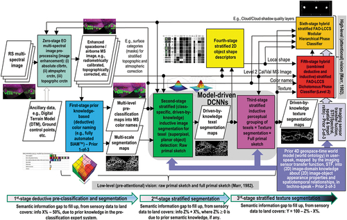
In compliance with requirements (6.i) to (6.iii) expressed above, a structured hierarchical hybrid feedback CV system design (architecture) is shown in Figure 34. Originally proposed in (Baraldi, 2017; Baraldi & Boschetti, 2012a, 2012b; Baraldi et al., 2014, 2018a, 2018b; Baraldi & Tiede, 2018a, 2018b), it adopts a convergence-of-evidence approach to ‘AGI ⊃ CV ⊃ EO-IU ⊃ ARD’ problems, where Equation (12)(12) $\begin{array}{rl}& \mathrm{M}\mathrm{I}\mathrm{N}\left\{\begin{array}{c}\mathrm{m}\left(\mathrm{C}\mathrm{o}\mathrm{l}\mathrm{o}\mathrm{r}\mathrm{V}\mathrm{a}\mathrm{l}\mathrm{u}\mathrm{e}\left(\mathrm{x}\right)|\mathrm{c}\right),\mathrm{m}\left(\mathrm{S}\mathrm{i}\mathrm{z}\mathrm{e}\mathrm{V}\mathrm{a}\mathrm{l}\mathrm{u}\mathrm{e}\left(\mathrm{x}\right)|\mathrm{c}\right),\\ \mathrm{m}\left(2\mathrm{D}\mathrm{s}\mathrm{h}\mathrm{a}\mathrm{p}\mathrm{e}\mathrm{V}\mathrm{a}\mathrm{l}\mathrm{u}\mathrm{e}\left(\mathrm{x}\right)|\mathrm{c}\right),\mathrm{m}\left(\mathrm{T}\mathrm{e}\mathrm{x}\mathrm{t}\mathrm{u}\mathrm{r}\mathrm{e}\mathrm{V}\mathrm{a}\mathrm{l}\mathrm{u}\mathrm{e}\left(\mathrm{x}\right)|\mathrm{c}\right),\\ \mathrm{m}\left(2\mathrm{D}\mathrm{s}\mathrm{p}\mathrm{a}\mathrm{t}\mathrm{i}\mathrm{a}\mathrm{l}\mathrm{R}\mathrm{e}\mathrm{l}\mathrm{a}\mathrm{t}\mathrm{i}\mathrm{o}\mathrm{n}\mathrm{s}\mathrm{h}\mathrm{i}\mathrm{p}\mathrm{s}\left(\mathrm{x},2\mathrm{D}\mathrm{n}\mathrm{e}\mathrm{i}\mathrm{g}\mathrm{h}\left(\mathrm{x}\right)\right)|\mathrm{c}\right)\end{array}\right\}\\ & =\mathrm{M}\mathrm{I}\mathrm{N}\left\{\begin{array}{c}\sum _{\mathrm{C}\mathrm{o}\mathrm{l}\mathrm{o}\mathrm{r}\mathrm{N}\mathrm{a}\mathrm{m}{\mathrm{e}}_{\mathrm{j}},\mathrm{e}.\mathrm{g}.,\mathrm{r}\mathrm{e}\mathrm{d},\mathrm{g}\mathrm{r}\mathrm{e}\mathrm{e}\mathrm{n},\mathrm{b}\mathrm{l}\mathrm{u}\mathrm{e},\mathrm{e}\mathrm{t}\mathrm{c}.,\mathrm{w}\mathrm{i}\mathrm{t}\mathrm{h}\mathrm{j}=1}^{\mathrm{C}\mathrm{o}\mathrm{l}\mathrm{o}\mathrm{r}\mathrm{V}\mathrm{o}\mathrm{c}\mathrm{a}\mathrm{b}\mathrm{u}\mathrm{l}\mathrm{a}\mathrm{r}\mathrm{y}\mathrm{C}\mathrm{a}\mathrm{r}\mathrm{d}\mathrm{i}\mathrm{n}\mathrm{a}\mathrm{l}\mathrm{i}\mathrm{t}\mathrm{y}}\\ \mathrm{m}\left(\mathrm{C}\mathrm{o}\mathrm{l}\mathrm{o}\mathrm{r}\mathrm{V}\mathrm{a}\mathrm{l}\mathrm{u}\mathrm{e}\left(\mathrm{x}\right)|\mathrm{C}\mathrm{o}\mathrm{l}\mathrm{o}\mathrm{r}\mathrm{N}\mathrm{a}\mathrm{m}{\mathrm{e}}_{\mathrm{j}}\right)\mathrm{m}\left(\mathrm{C}\mathrm{o}\mathrm{l}\mathrm{o}\mathrm{r}\mathrm{N}\mathrm{a}\mathrm{m}{\mathrm{e}}_{\mathrm{j}}|\mathrm{c}\right),\\ \mathrm{m}\left(\mathrm{S}\mathrm{i}\mathrm{z}\mathrm{e}\mathrm{V}\mathrm{a}\mathrm{l}\mathrm{u}\mathrm{e}\left(\mathrm{x}\right)|\mathrm{c}\right),\mathrm{m}\left(2\mathrm{D}\mathrm{s}\mathrm{h}\mathrm{a}\mathrm{p}\mathrm{e}\mathrm{V}\mathrm{a}\mathrm{l}\mathrm{u}\mathrm{e}\left(\mathrm{x}\right)|\mathrm{c}\right),\\ \mathrm{m}\left(\mathrm{T}\mathrm{e}\mathrm{x}\mathrm{t}\mathrm{u}\mathrm{r}\mathrm{e}\mathrm{V}\mathrm{a}\mathrm{l}\mathrm{u}\mathrm{e}\left(\mathrm{x}\right)|\mathrm{c}\right),\\ \mathrm{m}\left(2\mathrm{D}\mathrm{s}\mathrm{p}\mathrm{a}\mathrm{t}\mathrm{i}\mathrm{a}\mathrm{l}\mathrm{R}\mathrm{e}\mathrm{l}\mathrm{a}\mathrm{t}\mathrm{i}\mathrm{o}\mathrm{n}\mathrm{s}\mathrm{h}\mathrm{i}\mathrm{p}\mathrm{s}\left(\mathrm{x},2\mathrm{D}\mathrm{n}\mathrm{e}\mathrm{i}\mathrm{g}\mathrm{h}\left(\mathrm{x}\right)\right)|\mathrm{c}\right)\end{array}\right\}\\ & =\mathrm{M}\mathrm{I}\mathrm{N}\{\mathrm{m}\left(\mathrm{C}\mathrm{o}\mathrm{l}\mathrm{o}\mathrm{r}\mathrm{N}\mathrm{a}\mathrm{m}{\mathrm{e}}^{\ast }|\mathrm{c}\right)\in \left\{0,1\right\},\mathrm{m}\left(\mathrm{S}\mathrm{i}\mathrm{z}\mathrm{e}\mathrm{V}\mathrm{a}\mathrm{l}\mathrm{u}\mathrm{e}\left(\mathrm{x}\right)|\mathrm{c}\right)\in \left[0.0,1.0\right],\\ & \mathrm{m}\left(2\mathrm{D}\mathrm{s}\mathrm{h}\mathrm{a}\mathrm{p}\mathrm{e}\mathrm{V}\mathrm{a}\mathrm{l}\mathrm{u}\mathrm{e}\left(\mathrm{x}\right)|\mathrm{c}\right)\in \left[0.0,1.0\right],\mathrm{m}\left(\mathrm{T}\mathrm{e}\mathrm{x}\mathrm{t}\mathrm{u}\mathrm{r}\mathrm{e}\mathrm{V}\mathrm{a}\mathrm{l}\mathrm{u}\mathrm{e}\left(\mathrm{x}\right)|\mathrm{c}\right)\in \left[0.0,1.0\right],\\ & \mathrm{m}\left(2\mathrm{D}\mathrm{s}\mathrm{p}\mathrm{a}\mathrm{t}\mathrm{i}\mathrm{a}\mathrm{l}\mathrm{R}\mathrm{e}\mathrm{l}\mathrm{a}\mathrm{t}\mathrm{i}\mathrm{o}\mathrm{n}\mathrm{s}\mathrm{h}\mathrm{i}\mathrm{p}\mathrm{s}\left(\mathrm{x},2\mathrm{D}\mathrm{n}\mathrm{e}\mathrm{i}\mathrm{g}\mathrm{h}\left(\mathrm{x}\right)\right)|\mathrm{c}\right)\in \left[0.0,1.0\right]\}\end{array}$(12) is enforced as naïve Bayes classification paradigm. Worth noting, in this CV system design, relationship ‘Deductive (physical model-based, ‘hand-crafted’) DCNN → Hybrid feedback CV’ holds; it means that a deductive multi-scale multi-orientation DCNN (see Figure 28) is included (as part-of, without inheritance) in the proposed CV system. Hence, the proposed hybrid feedback CV system outpaces the “complexity” of traditional inductive feedforward DCNNs. Moreover, this CV system design is in contrast with the recent hype on ‘DCNN ⊃ DL ⊃ ML’, where an inductive end-to-end feedforward DCNN is typically considered, per se (on a standalone basis), equivalent to a whole CV system (Cimpoi et al., 2014; Krizhevsky et al., 2012). The popular belief that relationship ‘Inductive end-to-end feedforward DCNN = CV’ holds is yet-another instantiation of the erroneous belief that Equation (7)(7) $\text{lsquo}\mathrm{A}(\mathrm{G}/\mathrm{N})\mathrm{I}\supset \mathrm{M}\mathrm{L}\supset \mathrm{D}\mathrm{L}\supset \mathrm{D}\mathrm{C}\mathrm{N}\mathrm{N}\text{rsquo}$(7) = ‘DCNN ⊂ DL ⊂ ML ⊂ A(G/N)I’ holds true (Claire, 2019; Copeland, 2016), see Figure 11(c).

In the proposed six-stage hybrid feedback ‘CV ⊃ EO-IU ⊃ ARD’ system architecture depicted in Figure 34, at Stage one, acronym SIAM (refer to references listed in Section 2) identifies a lightweight computer program, suitable for running on web services and/or mobile devices, such as tablet computers and smartphones, capable of: (i) MS reflectance space hyperpolyhedralization into a static vocabulary of MS color names (see Figure 2, Figure 29, Figure 30 and Figure 32), (ii) superpixel detection, by means of a well-posed two-pass connected-component multi-level image labeling algorithm (Dillencourt et al., 1992; Sonka et al., 1994) (see Figure 31), and (iii) vector quantization (VQ) quality assessment, see Figure 28. Stages numbered from zero to four cope with driven-by-prior-knowledge/ class-conditional/ Bayesian visual feature extraction. Stage five and Stage six deal with a hierarchical approach to EO image understanding (classification). In more detail, Stage five pursues a general-purpose, sensor-, application- and user-independent EO image classification first phase, consistent with the standard fully-nested 3-level 8-class FAO LCCS-DP taxonomy (Di Gregorio & Jansen, 2000), see Figure 3. In a hierarchical sequence with Stage five, Stage six is responsible of specialized, application-dependent and user-dependent EO image classification tasks, consistent with the standard fully-nested FAO LCCS-MHP taxonomy (Di Gregorio & Jansen, 2000), see Figure 3. In agreement with Equation (12)(12) $\begin{array}{rl}& \mathrm{M}\mathrm{I}\mathrm{N}\left\{\begin{array}{c}\mathrm{m}\left(\mathrm{C}\mathrm{o}\mathrm{l}\mathrm{o}\mathrm{r}\mathrm{V}\mathrm{a}\mathrm{l}\mathrm{u}\mathrm{e}\left(\mathrm{x}\right)|\mathrm{c}\right),\mathrm{m}\left(\mathrm{S}\mathrm{i}\mathrm{z}\mathrm{e}\mathrm{V}\mathrm{a}\mathrm{l}\mathrm{u}\mathrm{e}\left(\mathrm{x}\right)|\mathrm{c}\right),\\ \mathrm{m}\left(2\mathrm{D}\mathrm{s}\mathrm{h}\mathrm{a}\mathrm{p}\mathrm{e}\mathrm{V}\mathrm{a}\mathrm{l}\mathrm{u}\mathrm{e}\left(\mathrm{x}\right)|\mathrm{c}\right),\mathrm{m}\left(\mathrm{T}\mathrm{e}\mathrm{x}\mathrm{t}\mathrm{u}\mathrm{r}\mathrm{e}\mathrm{V}\mathrm{a}\mathrm{l}\mathrm{u}\mathrm{e}\left(\mathrm{x}\right)|\mathrm{c}\right),\\ \mathrm{m}\left(2\mathrm{D}\mathrm{s}\mathrm{p}\mathrm{a}\mathrm{t}\mathrm{i}\mathrm{a}\mathrm{l}\mathrm{R}\mathrm{e}\mathrm{l}\mathrm{a}\mathrm{t}\mathrm{i}\mathrm{o}\mathrm{n}\mathrm{s}\mathrm{h}\mathrm{i}\mathrm{p}\mathrm{s}\left(\mathrm{x},2\mathrm{D}\mathrm{n}\mathrm{e}\mathrm{i}\mathrm{g}\mathrm{h}\left(\mathrm{x}\right)\right)|\mathrm{c}\right)\end{array}\right\}\\ & =\mathrm{M}\mathrm{I}\mathrm{N}\left\{\begin{array}{c}\sum _{\mathrm{C}\mathrm{o}\mathrm{l}\mathrm{o}\mathrm{r}\mathrm{N}\mathrm{a}\mathrm{m}{\mathrm{e}}_{\mathrm{j}},\mathrm{e}.\mathrm{g}.,\mathrm{r}\mathrm{e}\mathrm{d},\mathrm{g}\mathrm{r}\mathrm{e}\mathrm{e}\mathrm{n},\mathrm{b}\mathrm{l}\mathrm{u}\mathrm{e},\mathrm{e}\mathrm{t}\mathrm{c}.,\mathrm{w}\mathrm{i}\mathrm{t}\mathrm{h}\mathrm{j}=1}^{\mathrm{C}\mathrm{o}\mathrm{l}\mathrm{o}\mathrm{r}\mathrm{V}\mathrm{o}\mathrm{c}\mathrm{a}\mathrm{b}\mathrm{u}\mathrm{l}\mathrm{a}\mathrm{r}\mathrm{y}\mathrm{C}\mathrm{a}\mathrm{r}\mathrm{d}\mathrm{i}\mathrm{n}\mathrm{a}\mathrm{l}\mathrm{i}\mathrm{t}\mathrm{y}}\\ \mathrm{m}\left(\mathrm{C}\mathrm{o}\mathrm{l}\mathrm{o}\mathrm{r}\mathrm{V}\mathrm{a}\mathrm{l}\mathrm{u}\mathrm{e}\left(\mathrm{x}\right)|\mathrm{C}\mathrm{o}\mathrm{l}\mathrm{o}\mathrm{r}\mathrm{N}\mathrm{a}\mathrm{m}{\mathrm{e}}_{\mathrm{j}}\right)\mathrm{m}\left(\mathrm{C}\mathrm{o}\mathrm{l}\mathrm{o}\mathrm{r}\mathrm{N}\mathrm{a}\mathrm{m}{\mathrm{e}}_{\mathrm{j}}|\mathrm{c}\right),\\ \mathrm{m}\left(\mathrm{S}\mathrm{i}\mathrm{z}\mathrm{e}\mathrm{V}\mathrm{a}\mathrm{l}\mathrm{u}\mathrm{e}\left(\mathrm{x}\right)|\mathrm{c}\right),\mathrm{m}\left(2\mathrm{D}\mathrm{s}\mathrm{h}\mathrm{a}\mathrm{p}\mathrm{e}\mathrm{V}\mathrm{a}\mathrm{l}\mathrm{u}\mathrm{e}\left(\mathrm{x}\right)|\mathrm{c}\right),\\ \mathrm{m}\left(\mathrm{T}\mathrm{e}\mathrm{x}\mathrm{t}\mathrm{u}\mathrm{r}\mathrm{e}\mathrm{V}\mathrm{a}\mathrm{l}\mathrm{u}\mathrm{e}\left(\mathrm{x}\right)|\mathrm{c}\right),\\ \mathrm{m}\left(2\mathrm{D}\mathrm{s}\mathrm{p}\mathrm{a}\mathrm{t}\mathrm{i}\mathrm{a}\mathrm{l}\mathrm{R}\mathrm{e}\mathrm{l}\mathrm{a}\mathrm{t}\mathrm{i}\mathrm{o}\mathrm{n}\mathrm{s}\mathrm{h}\mathrm{i}\mathrm{p}\mathrm{s}\left(\mathrm{x},2\mathrm{D}\mathrm{n}\mathrm{e}\mathrm{i}\mathrm{g}\mathrm{h}\left(\mathrm{x}\right)\right)|\mathrm{c}\right)\end{array}\right\}\\ & =\mathrm{M}\mathrm{I}\mathrm{N}\{\mathrm{m}\left(\mathrm{C}\mathrm{o}\mathrm{l}\mathrm{o}\mathrm{r}\mathrm{N}\mathrm{a}\mathrm{m}{\mathrm{e}}^{\ast }|\mathrm{c}\right)\in \left\{0,1\right\},\mathrm{m}\left(\mathrm{S}\mathrm{i}\mathrm{z}\mathrm{e}\mathrm{V}\mathrm{a}\mathrm{l}\mathrm{u}\mathrm{e}\left(\mathrm{x}\right)|\mathrm{c}\right)\in \left[0.0,1.0\right],\\ & \mathrm{m}\left(2\mathrm{D}\mathrm{s}\mathrm{h}\mathrm{a}\mathrm{p}\mathrm{e}\mathrm{V}\mathrm{a}\mathrm{l}\mathrm{u}\mathrm{e}\left(\mathrm{x}\right)|\mathrm{c}\right)\in \left[0.0,1.0\right],\mathrm{m}\left(\mathrm{T}\mathrm{e}\mathrm{x}\mathrm{t}\mathrm{u}\mathrm{r}\mathrm{e}\mathrm{V}\mathrm{a}\mathrm{l}\mathrm{u}\mathrm{e}\left(\mathrm{x}\right)|\mathrm{c}\right)\in \left[0.0,1.0\right],\\ & \mathrm{m}\left(2\mathrm{D}\mathrm{s}\mathrm{p}\mathrm{a}\mathrm{t}\mathrm{i}\mathrm{a}\mathrm{l}\mathrm{R}\mathrm{e}\mathrm{l}\mathrm{a}\mathrm{t}\mathrm{i}\mathrm{o}\mathrm{n}\mathrm{s}\mathrm{h}\mathrm{i}\mathrm{p}\mathrm{s}\left(\mathrm{x},2\mathrm{D}\mathrm{n}\mathrm{e}\mathrm{i}\mathrm{g}\mathrm{h}\left(\mathrm{x}\right)\right)|\mathrm{c}\right)\in \left[0.0,1.0\right]\}\end{array}$(12) , independent sources of visual evidence to be considered as input to the EO image classification subsystem, comprising Stage five and Stage six in sequence, are (refer to this Subsection above): (i) numerical color values, discretized (quantized) into categorical color names by Stage one, (ii) individual image-objects, identified as raw primal sketch by Stage two (Baraldi, 2017; Marr, 1982), (iii) texture features, identified as full primal sketch by Stage three (Baraldi, 2017; Cherry, 2019; Geirhos et al., 2018; Green, 1997; Jain & Healey, 1998; Julesz, 1986; Julesz et al., 1973; Koffka, 1935; Marr, 1982; Tuceryan, 1992; Victor, 1994; Yellott, 1993), (iv) scale-invariant 2D shape indexes of image-objects (Baraldi, 2017; Baraldi & Soares, 2017), computed at Stage four, and (v) inter-object spatial relationships, either topological (e.g. adjacency, inclusion, etc.) or non-topological (e.g. spatial distance, orientation, etc.) (refer to this Subsection above).

5. Critical comparison of existing EO optical image-derived Level 2/ARD product definitions and software implementations

According to Section 2, in a new notion of Space Economy 4.0 (Mazzucato & Robinson, 2017), to comply with the standard set of FAIR guiding principles for scientific data (product and process) management (GO FAIR – International Support and Coordination Office, 2021; Wilkinson et al., 2016) (see Table 1), EO large image databases, characterized by the six Vs of volume, variety, veracity, velocity, volatility and value (Metternicht et al., 2020), are transformed at the space segment and/or midstream segment (see Figure 10) into multi-source EO sensory image-derived Level 2/ARD information products of scientific quality (NASA – National Aeronautics and Space Administration, 2019; CEOS – Committee on Earth Observation Satellites, 2018; DLR – Deutsches Zentrum für Luft-und Raumfahrt e.V. and VEGA Technologies, 2011; Dwyer et al., 2018; ESA – European Space Agency, 2015; Gómez-Chova et al., 2007; Helder et al., 2018; Houborga & McCabe, 2018; OHB, 2016; USGS – U.S. Geological Survey, 2018a, 2018b, 2018c; Vermote & Saleous, 2007), consisting of numerical variable co-product(s) in raster graphics format stacked with symbolic (categorical and semantic) information co-product(s), such as SCMs, in raster or vector graphics format(s), ready to be analyzed quantitatively by the downstream segment for systematic, timely, operational and comprehensive generation of VAPS at an expected level of precision (vice versa, uncertainty), in agreement with the intergovernmental GEO-CEOS QA4EO Cal/Val guidelines (refer to references listed in Section 2). For EO sensory image-derived ARD-specific information products (outcomes) and processes, semantic relationship ‘ARD ⊂ EO-IU ⊂ CV ⊂ AGI’ = Equation (3)(3) $\text{lsquo}\mathrm{A}\mathrm{R}\mathrm{D}\subset \mathrm{E}\mathrm{O}-\mathrm{I}\mathrm{U}\subset \mathrm{C}\mathrm{V}\subset \mathrm{A}\mathrm{G}\mathrm{I}\subset \mathrm{C}\mathrm{o}\mathrm{g}\mathrm{n}\mathrm{i}\mathrm{t}\mathrm{i}\mathrm{v}\mathrm{e}\mathrm{s}\mathrm{c}\mathrm{i}\mathrm{e}\mathrm{n}\mathrm{c}\mathrm{e}\text{rsquo}$(3) holds, where specialization with inheritance increases from right to left.

In Section 2, the potential impact of systematic, timely, comprehensive and operational generation of a multi-source semantics-enriched ARD product-pair at the space segment and/or midstream segment upon a new notion of Space Economy 4.0 (see Figure 10) is highlighted by considering that the concept of ARD, provided with quality layers to manage data uncertainty (vice versa, veracity), has been strictly coupled with the increasingly popular notion of EO (raster-based) data cube, proposed as innovative midstream EO technology by the RS community in recent years (Open Data Cube, 2020; Baumann, 2017; CEOS – Committee on Earth Observation Satellites, 2020; Giuliani et al., 2017, 2020; Lewis et al., 2017; Strobl et al., 2017).

Unfortunately, as pointed out in Section 2, a community-agreed definition of EO big data cube does not exist yet, although several recommendations and implementations have been proposed (Open Data Cube, 2020; Baumann, 2017; CEOS – Committee on Earth Observation Satellites, 2020; Giuliani et al., 2017, 2020; Lewis et al., 2017; Strobl et al., 2017). A community-agreed definition of ARD, to be adopted as standard baseline in EO (raster-based) data cubes, does not exist either. As a consequence, in the RS common practice, many EO (raster-based) data cube definitions and implementations do not require ARD to run and, vice versa, an ever-increasing ensemble of new (supposedly better) ARD definitions and/or ARD-specific software implementations is proposed by the RS community (Bilal et al., 2019; CEOS – Committee on Earth Observation Satellites, 2018; DLR – Deutsches Zentrum für Luft-und Raumfahrt e.V. and VEGA Technologies, 2011; Dwyer et al., 2018; ESA – European Space Agency, 2015; Helder et al., 2018; NASA – National Aeronautics and Space Administration, 2019; Qiu et al., 2019; USGS – U.S. Geological Survey, 2018a, 2018b, 2018c; Vermote & Saleous, 2007), independently of a standardized/harmonized definition of EO big data cube.

Based on working hypothesis ‘ARD ⊂ EO-IU ⊂ CV ⊂ AGI’ = Equation (3)(3) $\text{lsquo}\mathrm{A}\mathrm{R}\mathrm{D}\subset \mathrm{E}\mathrm{O}-\mathrm{I}\mathrm{U}\subset \mathrm{C}\mathrm{V}\subset \mathrm{A}\mathrm{G}\mathrm{I}\subset \mathrm{C}\mathrm{o}\mathrm{g}\mathrm{n}\mathrm{i}\mathrm{t}\mathrm{i}\mathrm{v}\mathrm{e}\mathrm{s}\mathrm{c}\mathrm{i}\mathrm{e}\mathrm{n}\mathrm{c}\mathrm{e}\text{rsquo}$(3) , the present Section focuses on the open problem of ARD product (outcome) and process standardization/harmonization to promote the well-known FAIR guiding principles for scientific data (product and process) management (GO FAIR – International Support and Coordination Office, 2021; Wilkinson et al., 2016) (see Table 1) in the “seamless innovation chain” required by a new notion of Space Economy 4.0 (see Figure 10), where system reusability and system interoperability (intended as 1^st communication level, 2^nd syntax level and 3^rd semantic/ontological level of system interoperability, refer to Section 2) are regarded as pre-conditions to semantics-enabled data and data-derived information findability, accessibility and reusability, see Equation (1)(1) $\begin{array}{rl}& \text{lsquo}\mathrm{A}\mathrm{G}\mathrm{I}\text{-}\mathrm{e}\mathrm{n}\mathrm{a}\mathrm{b}\mathrm{l}\mathrm{e}\mathrm{d}\mathrm{D}\mathrm{I}\mathrm{A}\mathrm{S}=\mathrm{A}\mathrm{G}\mathrm{I}4\mathrm{D}\mathrm{I}\mathrm{A}\mathrm{S}=\mathrm{S}\mathrm{e}\mathrm{m}\mathrm{a}\mathrm{n}\mathrm{t}\mathrm{i}\mathrm{c}\mathrm{s}\text{-}\mathrm{e}\mathrm{n}\mathrm{a}\mathrm{b}\mathrm{l}\mathrm{e}\mathrm{d}\mathrm{D}\mathrm{I}\mathrm{A}\mathrm{S}2.0\\ & (\mathrm{D}\mathrm{I}\mathrm{A}\mathrm{S}{2}^{\mathrm{n}\mathrm{d}}\mathrm{g}\mathrm{e}\mathrm{n}\mathrm{e}\mathrm{r}\mathrm{a}\mathrm{t}\mathrm{i}\mathrm{o}\mathrm{n})=\mathrm{D}\mathrm{I}\mathrm{A}\mathrm{S}2.0=\mathrm{A}\mathrm{G}\mathrm{I}+\mathrm{D}\mathrm{I}\mathrm{A}\mathrm{S}1.0+\mathrm{S}\mathrm{C}\mathrm{B}\mathrm{I}\mathrm{R}+\mathrm{S}\mathrm{E}\mathrm{I}\mathrm{K}\mathrm{D}\text{rsquo}\end{array}$(1) = AGI4DIAS.

Figure 35. Comparison of existing EO sensory data-derived Level 2/Analysis Ready Data (ARD) information products, where dimensionless digital numbers (DNs ≥ 0) at Level 0 have been radiometrically corrected (calibrated) into top-of-atmosphere reflectance (TOARF) values in range [0.0, 1.0] at Level 1, whereas TOARF values at Level 1 are corrected from atmospheric and, eventually, topographic and adjacency effects into surface reflectance (SURF) values, belonging to range [0.0, 1.0], at Level 2 (Egorov, Roy, Zhang, Hansen, and Kommareddy, 2018). Adopted acronyms: Committee on Earth Observation Satellites (CEOS) ARD for Land (CARD4L) product definition (CEOS – Committee on Earth Observation Satellites, 2018); U.S. Geological Survey (USGS)-National Aeronautics and Space Administration (NASA) Landsat Ecosystem Disturbance Adaptive Processing System (LEDAPS) software executable for Landsat-4/-5/-7 imagery (Vermote & Saleous, 2007), plus Landsat Surface Reflectance Code (LaSRC) software executable for Landsat-8 imagery (Bilal et al., 2019; Qiu et al., 2019; USGS – U.S. Geological Survey, 2018b); Italian Space Agency (ASI) Hyperspectral Precursor and Application Mission (PRISMA) imaging sensor (ASI – Agenzia Spaziale Italiana, 2020; OHB, 2016); European Space Agency (ESA) EO Sentinel-2 data-derived Level 2 product, generated by the Sentinel 2 (atmospheric, topographic and adjacency) Correction Prototype Processor (Sen2Cor) (DLR – Deutsches Zentrum für Luft-und Raumfahrt e.V. and VEGA Technologies, 2011; ESA – European Space Agency, 2015). More acronyms adopted in this table: Digital Elevation Model (DEM), open source C Function of Mask (CFMask) algorithm (USGS – U.S. Geological Survey, 2018a, 2018c).

The original contribution of this Section is twofold. First, it provides a critical assessment and inter-comparison of four existing EO optical image-derived Level 2/ARD product definitions and four ARD-specific software implementations, investigated at the Marr five levels of system understanding (refer to Subsection 3.2). Second, an innovative, ambitious (more informative), but realistic (feasible) semantics-enriched ‘ARD ⊂ EO-IU ⊂ CV ⊂ AGI’ product-pair and process gold standard is proposed for implementation at the space segment, referred to as AGI4Space, and/or midstream segment, referred to as AGI4DIAS = Equation (1)(1) $\begin{array}{rl}& \text{lsquo}\mathrm{A}\mathrm{G}\mathrm{I}\text{-}\mathrm{e}\mathrm{n}\mathrm{a}\mathrm{b}\mathrm{l}\mathrm{e}\mathrm{d}\mathrm{D}\mathrm{I}\mathrm{A}\mathrm{S}=\mathrm{A}\mathrm{G}\mathrm{I}4\mathrm{D}\mathrm{I}\mathrm{A}\mathrm{S}=\mathrm{S}\mathrm{e}\mathrm{m}\mathrm{a}\mathrm{n}\mathrm{t}\mathrm{i}\mathrm{c}\mathrm{s}\text{-}\mathrm{e}\mathrm{n}\mathrm{a}\mathrm{b}\mathrm{l}\mathrm{e}\mathrm{d}\mathrm{D}\mathrm{I}\mathrm{A}\mathrm{S}2.0\\ & (\mathrm{D}\mathrm{I}\mathrm{A}\mathrm{S}{2}^{\mathrm{n}\mathrm{d}}\mathrm{g}\mathrm{e}\mathrm{n}\mathrm{e}\mathrm{r}\mathrm{a}\mathrm{t}\mathrm{i}\mathrm{o}\mathrm{n})=\mathrm{D}\mathrm{I}\mathrm{A}\mathrm{S}2.0=\mathrm{A}\mathrm{G}\mathrm{I}+\mathrm{D}\mathrm{I}\mathrm{A}\mathrm{S}1.0+\mathrm{S}\mathrm{C}\mathrm{B}\mathrm{I}\mathrm{R}+\mathrm{S}\mathrm{E}\mathrm{I}\mathrm{K}\mathrm{D}\text{rsquo}\end{array}$(1) , see Figure 10.

Noteworthy, since semantic relationship ‘ARD ⊂ EO-IU ⊂ CV ⊂ AGI’ = Equation (3)(3) $\text{lsquo}\mathrm{A}\mathrm{R}\mathrm{D}\subset \mathrm{E}\mathrm{O}-\mathrm{I}\mathrm{U}\subset \mathrm{C}\mathrm{V}\subset \mathrm{A}\mathrm{G}\mathrm{I}\subset \mathrm{C}\mathrm{o}\mathrm{g}\mathrm{n}\mathrm{i}\mathrm{t}\mathrm{i}\mathrm{v}\mathrm{e}\mathrm{s}\mathrm{c}\mathrm{i}\mathrm{e}\mathrm{n}\mathrm{c}\mathrm{e}\text{rsquo}$(3) holds then, in agreement with a Bayesian inference approach to data analysis (Bowers & Davis, 2012; Ghahramani, 2011; Lähteenlahti, 2021; Quinlan, 2012; Sarkar, 2018), the set of Bayesian constraints proposed in Subsection 4.2, to better condition an inherently ill-posed ‘EO-IU ⊂ CV ⊂ AGI’ system, can be further specialized for better conditioning an inherently ill-posed ARD-specific information-as-data-interpretation task.

5.1. Critical assessment and inter-comparison of four existing EO optical image-derived Level 2/ARD product definitions and four ARD-specific software implementations

In this Subsection, a comparison of four existing EO optical image-derived Level 2/ARD product definitions and four ARD-specific software implementations is proposed in Figure 35 and depicted in Figure 36 for critical assessment at the Marr five levels of system understanding (refer to Subsection 3.2). This original comparison reveals the following.

First, the ASI PRISMA data-derived Level 2 product definition and software implementation appear peculiar (ASI – Agenzia Spaziale Italiana, 2020; OHB, 2016), sometime more loose (relaxed, e.g. no Cloud-shadow quality layer detection is required, unlike the ESA Sentinel-2 Level 2 thematic co-product taxonomy (DLR – Deutsches Zentrum für Luft-und Raumfahrt e.V. and VEGA Technologies, 2011; ESA – European Space Agency, 2015)), but sometime stricter in requirements (e.g. more LC classes are investigated at the intermediate Level 1 semantic co-product, including LC class Forest and LC class Crop) than the remaining three Level 2/ARD product definitions. Noteworthy, the US Geological Survey (USGS)-NASA ARD definition (NASA – National Aeronautics and Space Administration, 2019; Dwyer et al., 2018; Helder et al., 2018; USGS – U.S. Geological Survey, 2018a, 2018c) is provided with two sensor series-specific software implementations, namely, the Landsat Ecosystem Disturbance Adaptive Processing System (LEDAPS) software executable for Landsat-4/-5/-7 imagery (Vermote & Saleous, 2007) and the Landsat Surface Reflectance Code (LaSRC) software executable for Landsat-8 imagery (Bilal et al., 2019; Qiu et al., 2019; USGS – U.S. Geological Survey, 2018b). The USGS-NASA ARD definition coincides with the ARD definition (without software implementation) proposed by the international Committee on Earth Observation Satellites (CEOS) in the ARD for Land Optical Surface Reflectance (CARD4L-OSR) initiative (CEOS – Committee on Earth Observation Satellites, 2018). Moreover, it is less restrictive/specialized than (it is superset-of) the ESA EO data-derived Level 2 product definition adopted by Sen2Cor, the sensor-specific Level 2 software implementation developed by ESA for Sentinel-2 imagery, run by ESA and/or distributed by ESA free-of-cost to be run on the user side (DLR – Deutsches Zentrum für Luft-und Raumfahrt e.V. and VEGA Technologies, 2011; ESA – European Space Agency, 2015), see Figure 37 and Figure 38.

Figure 36. Comparison of the CEOS ARD for Land Optical Surface Reflectance (CARD4L-OSR) product definition (CEOS – Committee on Earth Observation Satellites, 2018), supported by no computer vision (CV) software implementation, with existing ARD product implementations, namely, USGS-NASA ARD, ESA EO Level 2 and ASI PRISMA Level 1 and Level 2, also refer to Figure 35.

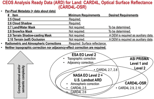
Second, the comparison proposed in Figures 35 and 36 shows that none of these four ARD/Level 2 product definitions complies with the Cloud/Not-Cloud = Rest-of-the-world taxonomy proposed to ESA by the Copernicus data Quality Control team for a third semantic/ontological level of interoperability of EO sensory-data derived Level 1 and Level 2/ARD products (ESA – European Space Agency, 2017a) (refer to Section 2).

Third, the comparison proposed in Figures 35 and 36 reveals that, among the four existing ARD/Level 2 product definitions, the more severe (constrained) and ambitious (informative) definition is the ESA Sentinel-2 data-specific Level 2 product-pair specification (DLR – Deutsches Zentrum für Luft-und Raumfahrt e.V. and VEGA Technologies, 2011; ESA – European Space Agency, 2015). The ESA Sentinel-2 sensor-specific Level 2 output product-pair definition is peculiar because twofold. It consists of one output quantitative/numerical (subsymbolic) variable co-product stacked (overlapped) with one output data-derived qualitative symbolic (categorical and semantic) variable co-product, referred to by ESA as SCM (DLR – Deutsches Zentrum für Luft-und Raumfahrt e.V. and VEGA Technologies, 2011; ESA – European Space Agency, 2015) (refer to Subsection 3.3.1). In more detail (see Figure 38), the two ESA Sentinel-2 sensor-specific Level 2 co-products consist of:

1. A single-date MS image, whose dimensionless DNs at Level 0, provided with no physical meaning and belonging to range DN ≥ 0 (refer to Subsection 3.3.2), have been radiometrically corrected (calibrated), in agreement with the GEO-CEOS QA4EO Cal guidelines, into TOARF values, belonging to range [0.0, 1.0], at Level 1; next, at Level 2, TOARF values at Level 1 are corrected in sequence from (i) atmospheric effects, from TOARF into SURF 1-of-3 values (refer to Subsection 3.3.2), (ii) topographic effects, from SURF 1-of-3 into SURF 2-of-3 values, and (iii) adjacency effects (Egorov, Roy, Zhang, Hansen, and Kommareddy, 2018), from SURF 2-of-3 into SURF 3-of-3 values, belonging to range [0.0, 1.0] (refer to Subsection 3.3.2),

   stacked (overlapped) with

2. A sensory image-derived general-purpose, user- and application-independent SCM (refer to Section 2), whose thematic map legend includes quality layers, such as Cloud and Cloud–shadow, see Figures 35 to 37. The non-standard sensor-specific general-purpose, user- and application-independent ESA Sen2Cor’s SCM taxonomy (DLR – Deutsches Zentrum für Luft-und Raumfahrt e.V. and VEGA Technologies, 2011; ESA – European Space Agency, 2015) is shown in Figure 37. It is alternative to both the non-standard Cloud versus Not-Cloud (Rest-of-the-world) taxonomy proposed to ESA by the Copernicus Data Quality Control team (ESA – European Space Agency, 2017a) (refer to Section 2) and the standard fully-nested FAO LCCS taxonomy (Di Gregorio & Jansen, 2000), see Figure 3. For structured system analysis at the Marr five levels of abstraction (refer to Subsection 3.2), the ESA Sen2Cor software system architecture is shown in Figure 38.

   Noteworthy, an SCM is included (referred to as land cover) in the list of terrestrial ECVs defined by the WCO (see Table 2), which complies with requirements of the GEO second implementation plan for years 2016–2025 of a new GEOSS, regarded as expert EO data-derived information and knowledge system (GEO – Group on Earth Observations, 2015; Nativi et al., 2015, 2020; Santoro et al., 2017) (see Figure 1), in agreement with the increasingly popular DIKW conceptual hierarchy (Rowley, 2007; Rowley & Hartley, 2008; Wikipedia, 2020a; Zeleny, 1987, 2005; Zins, 2007), see Figure 12 and Figure 16.

   Figure 37. Non-standard general-purpose, user- and application-independent European Space Agency (ESA) Earth observation (EO) Level 2 Scene Classification Map (SCM) legend adopted by the sensor-specific Sentinel 2 (atmospheric, adjacency and topographic) Correction (Sen2Cor) Prototype Processor (DLR – Deutsches Zentrum für Luft-und Raumfahrt e.V. and VEGA Technologies, 2011; ESA – European Space Agency, 2015), developed, run and/or distributed free-of-cost by ESA to be run on the user side. Noteworthy, the ESA Sen2Core SCM’s LC class taxonomy does not comply with a standard Food and Agriculture Organization (FAO) of the United Nations (UN) Land Cover Classification System (LCCS) taxonomy, which is fully nested and whose first-stage 3-level 8-class FAO LCCS Dichotomous Phase (DP) taxonomy is general-purpose, user- and application-independent, see Figure 3. This Sen2Cor’s SCM taxonomy is also alternative to the Cloud versus Not-Cloud (Rest-of-the-world) taxonomy proposed in the technical note “Harmonization of Cloud Classes” issued by the Copernicus Data Quality Control team (ESA – European Space Agency, 2017a) (refer to Section 2).

   

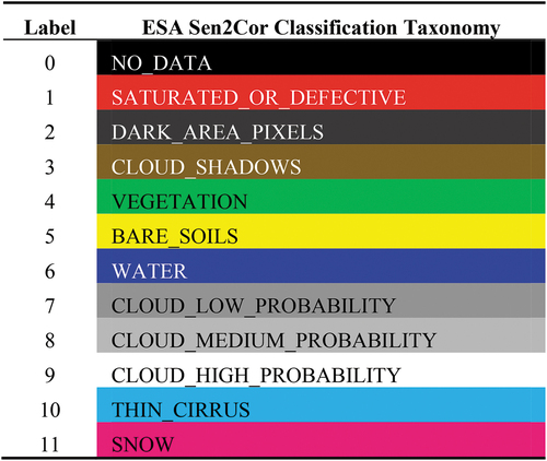
In more detail, Figure 38 shows that the ESA Sen2Cor SCM co-product generation is input with TOARF values. Since the ESA Sen2Cor SCM co-product is TOARF-derived, this SCM is not “aligned” with (it is not generated from) “new” better calibrated data available at the Sen2Cor output MS image co-product level, consisting of TOARF values radiometrically corrected into SURF 3-of-3 values (refer to Subsection 3.3.2). Since, typically, SURF ≠ TOARF, see Equation (9)(9) $\begin{array}{rl}& \text{lsquo}\mathrm{T}\mathrm{O}\mathrm{A}\mathrm{R}\mathrm{F}\approx \mathrm{S}\mathrm{U}\mathrm{R}\mathrm{F}\pm \mathrm{r}\mathrm{a}\mathrm{d}\mathrm{i}\mathrm{o}\mathrm{m}\mathrm{e}\mathrm{t}\mathrm{r}\mathrm{i}\mathrm{c}\mathrm{n}\mathrm{o}\mathrm{i}\mathrm{s}\mathrm{e}\mathrm{v}\mathrm{a}\mathrm{r}\mathrm{i}\mathrm{a}\mathrm{t}\mathrm{i}\mathrm{o}\mathrm{n}1,\mathrm{d}\mathrm{u}\mathrm{e}\mathrm{t}\mathrm{o}\mathrm{a}\mathrm{t}\mathrm{m}\mathrm{o}\mathrm{s}\mathrm{p}\mathrm{h}\mathrm{e}\mathrm{r}\mathrm{i}\mathrm{c}\mathrm{e}\mathrm{f}\mathrm{f}\mathrm{e}\mathrm{c}\mathrm{t}\mathrm{s},\\ & \pm \mathrm{r}\mathrm{a}\mathrm{d}\mathrm{i}\mathrm{o}\mathrm{m}\mathrm{e}\mathrm{t}\mathrm{r}\mathrm{i}\mathrm{c}\mathrm{n}\mathrm{o}\mathrm{i}\mathrm{s}\mathrm{e}\mathrm{v}\mathrm{a}\mathrm{r}\mathrm{i}\mathrm{a}\mathrm{t}\mathrm{i}\mathrm{o}\mathrm{n}2,\mathrm{d}\mathrm{u}\mathrm{e}\mathrm{t}\mathrm{o}\mathrm{t}\mathrm{o}\mathrm{p}\mathrm{o}\mathrm{g}\mathrm{r}\mathrm{a}\mathrm{p}\mathrm{h}\mathrm{i}\mathrm{c}\mathrm{e}\mathrm{f}\mathrm{f}\mathrm{e}\mathrm{c}\mathrm{t}\mathrm{s},\\ & \pm \mathrm{r}\mathrm{a}\mathrm{d}\mathrm{i}\mathrm{o}\mathrm{m}\mathrm{e}\mathrm{t}\mathrm{r}\mathrm{i}\mathrm{c}\mathrm{n}\mathrm{o}\mathrm{i}\mathrm{s}\mathrm{e}\mathrm{v}\mathrm{a}\mathrm{r}\mathrm{i}\mathrm{a}\mathrm{t}\mathrm{i}\mathrm{o}\mathrm{n}3,\mathrm{d}\mathrm{u}\mathrm{e}\mathrm{t}\mathrm{o}\mathrm{a}\mathrm{d}\mathrm{j}\mathrm{a}\mathrm{c}\mathrm{e}\mathrm{n}\mathrm{c}\mathrm{y}\mathrm{e}\mathrm{f}\mathrm{f}\mathrm{e}\mathrm{c}\mathrm{t}\mathrm{s},\pm \dots \text{rsquo}& (9)\end{array}$(9) , then a more ambitious, but missing SURF 3-of-3 data-derived SCM co-product would be expected to be different from the accomplished TOARF data-derived SCM co-product, made available to end-users. In practice, the Sen2Cor radiometric corrector of TOARF into SURF 1-of-3 to SURF 3-of-3 values employs the Sen2Cor SCM co-product for internal use as ancillary input map suitable for TOARF data stratification (masking) purposes, in line with a Bayesian inference approach to class-conditional data analysis (Bowers & Davis, 2012; Ghahramani, 2011; Lähteenlahti, 2021; Quinlan, 2012; Sarkar, 2018). Unfortunately, no “alignment” of the two ESA Sen2Cor output co-products to the same SURF 3-of-3 output values is pursued by the ESA Sen2Cor software, despite the fact that the Sen2Cor SCM decision-tree classifier, implemented to cope with input “noisy” TOARF values, is also capable of coping with input “noiseless” SURF 3-of-3 values as special case of TOARF values in clear-sky and flat-terrain conditions, since relationship ‘TOARF ≈ SURF 3-of-3 + atmospheric noise + topographic noise + adjacency noise effects + … ’ = Equation (9)(9) $\begin{array}{rl}& \text{lsquo}\mathrm{T}\mathrm{O}\mathrm{A}\mathrm{R}\mathrm{F}\approx \mathrm{S}\mathrm{U}\mathrm{R}\mathrm{F}\pm \mathrm{r}\mathrm{a}\mathrm{d}\mathrm{i}\mathrm{o}\mathrm{m}\mathrm{e}\mathrm{t}\mathrm{r}\mathrm{i}\mathrm{c}\mathrm{n}\mathrm{o}\mathrm{i}\mathrm{s}\mathrm{e}\mathrm{v}\mathrm{a}\mathrm{r}\mathrm{i}\mathrm{a}\mathrm{t}\mathrm{i}\mathrm{o}\mathrm{n}1,\mathrm{d}\mathrm{u}\mathrm{e}\mathrm{t}\mathrm{o}\mathrm{a}\mathrm{t}\mathrm{m}\mathrm{o}\mathrm{s}\mathrm{p}\mathrm{h}\mathrm{e}\mathrm{r}\mathrm{i}\mathrm{c}\mathrm{e}\mathrm{f}\mathrm{f}\mathrm{e}\mathrm{c}\mathrm{t}\mathrm{s},\\ & \pm \mathrm{r}\mathrm{a}\mathrm{d}\mathrm{i}\mathrm{o}\mathrm{m}\mathrm{e}\mathrm{t}\mathrm{r}\mathrm{i}\mathrm{c}\mathrm{n}\mathrm{o}\mathrm{i}\mathrm{s}\mathrm{e}\mathrm{v}\mathrm{a}\mathrm{r}\mathrm{i}\mathrm{a}\mathrm{t}\mathrm{i}\mathrm{o}\mathrm{n}2,\mathrm{d}\mathrm{u}\mathrm{e}\mathrm{t}\mathrm{o}\mathrm{t}\mathrm{o}\mathrm{p}\mathrm{o}\mathrm{g}\mathrm{r}\mathrm{a}\mathrm{p}\mathrm{h}\mathrm{i}\mathrm{c}\mathrm{e}\mathrm{f}\mathrm{f}\mathrm{e}\mathrm{c}\mathrm{t}\mathrm{s},\\ & \pm \mathrm{r}\mathrm{a}\mathrm{d}\mathrm{i}\mathrm{o}\mathrm{m}\mathrm{e}\mathrm{t}\mathrm{r}\mathrm{i}\mathrm{c}\mathrm{n}\mathrm{o}\mathrm{i}\mathrm{s}\mathrm{e}\mathrm{v}\mathrm{a}\mathrm{r}\mathrm{i}\mathrm{a}\mathrm{t}\mathrm{i}\mathrm{o}\mathrm{n}3,\mathrm{d}\mathrm{u}\mathrm{e}\mathrm{t}\mathrm{o}\mathrm{a}\mathrm{d}\mathrm{j}\mathrm{a}\mathrm{c}\mathrm{e}\mathrm{n}\mathrm{c}\mathrm{y}\mathrm{e}\mathrm{f}\mathrm{f}\mathrm{e}\mathrm{c}\mathrm{t}\mathrm{s},\pm \dots \text{rsquo}& (9)\end{array}$(9) holds (refer to Subsection 3.3.2).

Figure 38. Sensor-specific Sentinel 2 (atmospheric, adjacency and topographic) Correction (Sen2Cor) Prototype Processor (DLR – Deutsches Zentrum für Luft-und Raumfahrt e.V. and VEGA Technologies, 2011; ESA – European Space Agency, 2015), developed and distributed free-of-cost by ESA to be run on the user side. The Sen2Cor flow chart for ESA Level 2 product generation from Sentinel-2 imagery (DLR – Deutsches Zentrum für Luft-und Raumfahrt e.V. and VEGA Technologies, 2011; ESA – European Space Agency, 2015) is the same as that in the Atmospheric/Topographic Correction for Satellite Imagery (ATCOR) commercial software toolbox (Richter & Schläpfer, 2012). While sharing the same system design, ESA Sen2Cor and ATCOR differ at the two lowest levels of system abstraction, namely, algorithm and implementation (Marr, 1982) (refer to Subsection 3.2). First, a Scene Classification Map (SCM) is generated from top-of-atmosphere reflectance (TOARF) values. Next, class-conditional MS image radiometric enhancement of TOARF into surface reflectance (SURF) 3-of-3 values (refer to Subsection 3.3.2), synonym for bottom-of-atmosphere (BOA) reflectance values, corrected for atmospheric effects (into SURF 1-of-3 values), topographic effects (into SURF 2-of-3 values) and adjacency effects (into SURF 3-of-3 values), is accomplished in sequence (Egorov, Roy, Zhang, Hansen, and Kommareddy, 2018), stratified/ layered/ masked by the same SCM product generated at first stage from TOARF values. More acronyms in this figure: AOT = aerosol optical thickness, DEM = digital elevation model, LUT = look-up table. Noteworthy, in the ESA Sen2Cor software workflow, the output SCM co-product and the output MS image co-product are not “aligned” with each other. Whereas the output SCM co-product is generated from EO Level 1 data in TOARF values, the output MS image consists of Level 2 data in SURF 3-of-3 values, whose radiometric quality is better (in terms of robustness) than that of TOARF values available at Level 1. Hence, the output Level 2 MS image in SURF 3-of-3 values is eligible for better interpretation (classification), which would deliver as output a new Level 2 SURF 3-of-3 data-derived SCM co-product, whose symbolic mapping is “aligned” with the Level 2 data in SURF 3-of-3 values and whose semantic quality (in terms of semantic depth and/or semantic accuracy) is expected to be better than that of the Level 1 TOARF data-derived SCM actually provided as Level 2 output symbolic co-product.

To pursue third-level semantic/ontological interoperability and reusability in agreement with the FAIR principles (GO FAIR – International Support and Coordination Office, 2021; Wilkinson et al., 2016) (see Table 1), recent works in the RS literature (Baraldi, 2017; Baraldi & Tiede, 2018a, 2018b) recommended the aforementioned sensor-specific semantics-enriched ESA EO Level 2/ARD product-pair definition to be adopted systematically across EO imaging sensors as necessary-but-not-sufficient precondition to the development of a new generation of semantics-enabled EO big data cube management systems (Augustin et al., 2018, 2019; Baraldi, 2017; Baraldi & Tiede, 2018a, 2018b; Baraldi et al., 2016, 2017; FFG – Austrian Research Promotion Agency, 2015, 2016, 2018, 2020; Planet, 2018; Sudmanns et al., 2018; Tiede et al., 2017), synonym for semantics-enabled EO big raster-based numerical data and vector-based categorical (symbolic, semi-symbolic or sub-symbolic, see Figure 15 and refer to Subsection 3.3.1) information cube management system, in agreement with a new notion of AGI4DIAS = Equation (1)(1) $\begin{array}{rl}& \text{lsquo}\mathrm{A}\mathrm{G}\mathrm{I}\text{-}\mathrm{e}\mathrm{n}\mathrm{a}\mathrm{b}\mathrm{l}\mathrm{e}\mathrm{d}\mathrm{D}\mathrm{I}\mathrm{A}\mathrm{S}=\mathrm{A}\mathrm{G}\mathrm{I}4\mathrm{D}\mathrm{I}\mathrm{A}\mathrm{S}=\mathrm{S}\mathrm{e}\mathrm{m}\mathrm{a}\mathrm{n}\mathrm{t}\mathrm{i}\mathrm{c}\mathrm{s}\text{-}\mathrm{e}\mathrm{n}\mathrm{a}\mathrm{b}\mathrm{l}\mathrm{e}\mathrm{d}\mathrm{D}\mathrm{I}\mathrm{A}\mathrm{S}2.0\\ & (\mathrm{D}\mathrm{I}\mathrm{A}\mathrm{S}{2}^{\mathrm{n}\mathrm{d}}\mathrm{g}\mathrm{e}\mathrm{n}\mathrm{e}\mathrm{r}\mathrm{a}\mathrm{t}\mathrm{i}\mathrm{o}\mathrm{n})=\mathrm{D}\mathrm{I}\mathrm{A}\mathrm{S}2.0=\mathrm{A}\mathrm{G}\mathrm{I}+\mathrm{D}\mathrm{I}\mathrm{A}\mathrm{S}1.0+\mathrm{S}\mathrm{C}\mathrm{B}\mathrm{I}\mathrm{R}+\mathrm{S}\mathrm{E}\mathrm{I}\mathrm{K}\mathrm{D}\text{rsquo}\end{array}$(1) .

The concept of semantics-enabled EO big raster-based numerical data and vector-based categorical (symbolic, semi-symbolic or subsymbolic) information cube management system, synonym for AGI4DIAS = Equation (1)(1) $\begin{array}{rl}& \text{lsquo}\mathrm{A}\mathrm{G}\mathrm{I}\text{-}\mathrm{e}\mathrm{n}\mathrm{a}\mathrm{b}\mathrm{l}\mathrm{e}\mathrm{d}\mathrm{D}\mathrm{I}\mathrm{A}\mathrm{S}=\mathrm{A}\mathrm{G}\mathrm{I}4\mathrm{D}\mathrm{I}\mathrm{A}\mathrm{S}=\mathrm{S}\mathrm{e}\mathrm{m}\mathrm{a}\mathrm{n}\mathrm{t}\mathrm{i}\mathrm{c}\mathrm{s}\text{-}\mathrm{e}\mathrm{n}\mathrm{a}\mathrm{b}\mathrm{l}\mathrm{e}\mathrm{d}\mathrm{D}\mathrm{I}\mathrm{A}\mathrm{S}2.0\\ & (\mathrm{D}\mathrm{I}\mathrm{A}\mathrm{S}{2}^{\mathrm{n}\mathrm{d}}\mathrm{g}\mathrm{e}\mathrm{n}\mathrm{e}\mathrm{r}\mathrm{a}\mathrm{t}\mathrm{i}\mathrm{o}\mathrm{n})=\mathrm{D}\mathrm{I}\mathrm{A}\mathrm{S}2.0=\mathrm{A}\mathrm{G}\mathrm{I}+\mathrm{D}\mathrm{I}\mathrm{A}\mathrm{S}1.0+\mathrm{S}\mathrm{C}\mathrm{B}\mathrm{I}\mathrm{R}+\mathrm{S}\mathrm{E}\mathrm{I}\mathrm{K}\mathrm{D}\text{rsquo}\end{array}$(1) , is depicted in Figures 39 and 40. It is alternative to existing EO big (raster-based) data cube management systems including, first, the ensemble of implemented country-wide EO (raster-based) data cubes (Open Data Cube, 2020), such as the Digital Earth Africa, Digital Earth Australia (Lewis et al., 2017), Swiss Data Cube (Giuliani et al., 2017), etc. (Giuliani et al., 2020), where the CARD4L-OSR product definition (CEOS – Committee on Earth Observation Satellites, 2018) (see Figure 35) is adopted as standard ARD baseline, if any. Second, it is alternative to the family of five EC DIAS 1^st-generation (DIAS 1.0) instantiations (EU – European Union, 2017, 2018), where neither ARD definitions nor ARD-specific software implementations have ever been adopted in the pursuit of the standard FAIR principles for scientific data (product and process) management (refer to Section 2).

Figure 39. Semantics-enabled EO big raster-based (numerical) data and vector-based categorical (either subsymbolic, semi-symbolic or symbolic) information cube (Augustin et al., 2018, 2019; Baraldi et al., 2016, 2017; FFG – Austrian Research Promotion Agency, 2015, 2016, 2018, 2020; Sudmanns et al., 2021; Sudmanns et al., 2018; Tiede et al., 2017), synonym for artificial general intelligence (AGI) (Bills, 2020; Chollet, 2019; Dreyfus, 1965, 1991, 1992; EC – European Commission, 2019; Fjelland, 2020; Hassabis et al., 2017; Ideami, 2021; Jajal, 2018; Jordan, 2018; Mindfire Foundation, 2018; Practical AI, 2020; Romero, 2021; Santoro et al., 2021; Sweeney, 2018a; Wolski, 2020a, 2020b) for Data and Information Access Services (AGI4DIAS) = Equation (1)(1) $\begin{array}{rl}& \text{lsquo}\mathrm{A}\mathrm{G}\mathrm{I}\text{-}\mathrm{e}\mathrm{n}\mathrm{a}\mathrm{b}\mathrm{l}\mathrm{e}\mathrm{d}\mathrm{D}\mathrm{I}\mathrm{A}\mathrm{S}=\mathrm{A}\mathrm{G}\mathrm{I}4\mathrm{D}\mathrm{I}\mathrm{A}\mathrm{S}=\mathrm{S}\mathrm{e}\mathrm{m}\mathrm{a}\mathrm{n}\mathrm{t}\mathrm{i}\mathrm{c}\mathrm{s}\text{-}\mathrm{e}\mathrm{n}\mathrm{a}\mathrm{b}\mathrm{l}\mathrm{e}\mathrm{d}\mathrm{D}\mathrm{I}\mathrm{A}\mathrm{S}2.0\\ & (\mathrm{D}\mathrm{I}\mathrm{A}\mathrm{S}{2}^{\mathrm{n}\mathrm{d}}\mathrm{g}\mathrm{e}\mathrm{n}\mathrm{e}\mathrm{r}\mathrm{a}\mathrm{t}\mathrm{i}\mathrm{o}\mathrm{n})=\mathrm{D}\mathrm{I}\mathrm{A}\mathrm{S}2.0=\mathrm{A}\mathrm{G}\mathrm{I}+\mathrm{D}\mathrm{I}\mathrm{A}\mathrm{S}1.0+\mathrm{S}\mathrm{C}\mathrm{B}\mathrm{I}\mathrm{R}+\mathrm{S}\mathrm{E}\mathrm{I}\mathrm{K}\mathrm{D}\text{rsquo}\end{array}$(1) (see Figure 40), considered necessary-but-not-sufficient precondition to semantic content-based image retrieval (SCBIR) and semantics-enabled information/knowledge discovery (SEIKD) over heterogeneous data sources acquired through geospace-time and imaging sensors, where SCBIR and SEIKD are consistent with symbolic human reasoning in human-speak (Augustin et al., 2018, 2019; Baraldi, 2017; Baraldi & Tiede, 2018a, 2018b; Baraldi et al., 2016, 2017; Dhurba & King, 2005; Newell & Simon, 1972; Planet, 2018; Sudmanns et al., 2021; Sudmanns et al., 2018; Tiede et al., 2017), also refer to Figure 2 and Figure 10. When stored in the multi-source EO image database, any EO Level 0 image in dimensionless digital numbers (DNs), provided with no physical meaning, is automatically transformed by default into, first, a sensory-data derived single-date EO Level 1 image, radiometrically calibrated into top-of-atmosphere reflectance (TOARF) values. Next, it is automatically transformed by an ‘AGI ⊃ CV ⊃ EO-IU ⊃ ARD’ system in operational mode into an innovative semantics-enriched ARD co-product pair comprising: (i) a single-date multi-spectral (MS) image, radiometrically calibrated from TOARF into surface reflectance (SURF) values, corrected for atmospheric, adjacency and topographic effects, stacked with: (ii) its EO data-derived value-adding Scene Classification Map (SCM), equivalent to a sensory image-derived categorical/ nominal/ qualitative variable of semantic quality, where the thematic map legend, comprising quality layers such as Cloud and Cloud–shadow, is general-purpose, user- and application-independent. In practice, an SCM is an instantiation of one of the Essential Climate Variables (ECVs) defined by the World Climate Organization (WCO) for the terrestrial layer (Bojinski et al., 2014), namely, land cover (including vegetation types) (see Table 2), where ECVs are the EO data-derived value-adding information variables considered at the basis of the Information level in the Data-Information-Knowledge-Wisdom (DIKW) hierarchical conceptualization (Rowley, 2007; Rowley & Hartley, 2008; Wikipedia, 2020a; Zeleny, 1987, 2005; Zins, 2007) (see Figure 16) adopted by the GEO second implementation plan for years 2016–2025 of a Global Earth Observation System of (component) Systems (GEOSS) (GEO – Group on Earth Observations, 2015; Nativi et al., 2015, 2020; Santoro et al., 2017), see Figure 1. As a possible augmentation, this innovative semantics-enriched ARD co-product pair can be stacked with (iii) EO data-derived value-adding numerical variables, either: (I) biophysical variables, e.g. leaf area index (LAI) (Liang, 2004), aboveground biomass, etc., belonging to the set of ECVs defined by the WCO (Bojinski et al., 2014) (see Table 2), (II) class-conditional spectral indexes, e.g. vegetation class-conditional greenness index (Baraldi et al., 2010a, 2010b), and/or (III) categorical variables of subsymbolic quality (geographic field-objects) (Couclelis, 2010; Goodchild et al., 2007), e.g. fuzzy sets/discretization levels of a geographic field, such as fuzzy sets (Zadeh, 1965) low/ medium/ high of a numerical variable estimating speed, whether uncalibrated (dimensionless) or calibrated (provided with a physical unit of measure, say, km/h), etc. (Baraldi, 2017; Baraldi & Tiede, 2018a, 2018b). Unlike the proposed semantics-enabled EO big raster-based (numerical) data and vector-based (categorical) information cube management system, synonym for AGI4DIAS (see Figure 40), whose future developments depend on a more severe (more ambitious), but realistic multi-sensor EO optical sensory image-derived ARD co-product pair definition and software implementation to be community-agreed upon, existing operational country-wide EO (raster-based) data cubes, such as the Digital Earth Africa, Digital Earth Australia (Lewis et al., 2017), Swiss Data Cube (Giuliani et al., 2017), etc. (Giuliani et al., 2020), adopt the CEOS ARD for Land Optical Surface Reflectance (CARD4L-OSR) product definition as standard baseline (CEOS – Committee on Earth Observation Satellites, 2018) (see Figure 35), where an SCM is lacking as ARD symbolic co-product. As a consequence, they are affected by the data-rich information-poor (DRIP) syndrome (Ball, 2021; Bernus & Noran, 2017). In contrast with existing EO (raster-based) data cubes, systematic availability of an ARD symbolic co-product, namely, a sensory image-derived SCM co-product, is considered mandatory by a future generation of semantics-enabled EO raster-based data and vector-based information cube management systems (Augustin et al., 2018, 2019; Baraldi et al., 2017; FFG – Austrian Research Promotion Agency, 2015, 2016, 2018, 2020; Sudmanns et al., 2018; Tiede et al., 2017), synonym for AGI4DIAS = Equation (1)(1) $\begin{array}{rl}& \text{lsquo}\mathrm{A}\mathrm{G}\mathrm{I}\text{-}\mathrm{e}\mathrm{n}\mathrm{a}\mathrm{b}\mathrm{l}\mathrm{e}\mathrm{d}\mathrm{D}\mathrm{I}\mathrm{A}\mathrm{S}=\mathrm{A}\mathrm{G}\mathrm{I}4\mathrm{D}\mathrm{I}\mathrm{A}\mathrm{S}=\mathrm{S}\mathrm{e}\mathrm{m}\mathrm{a}\mathrm{n}\mathrm{t}\mathrm{i}\mathrm{c}\mathrm{s}\text{-}\mathrm{e}\mathrm{n}\mathrm{a}\mathrm{b}\mathrm{l}\mathrm{e}\mathrm{d}\mathrm{D}\mathrm{I}\mathrm{A}\mathrm{S}2.0\\ & (\mathrm{D}\mathrm{I}\mathrm{A}\mathrm{S}{2}^{\mathrm{n}\mathrm{d}}\mathrm{g}\mathrm{e}\mathrm{n}\mathrm{e}\mathrm{r}\mathrm{a}\mathrm{t}\mathrm{i}\mathrm{o}\mathrm{n})=\mathrm{D}\mathrm{I}\mathrm{A}\mathrm{S}2.0=\mathrm{A}\mathrm{G}\mathrm{I}+\mathrm{D}\mathrm{I}\mathrm{A}\mathrm{S}1.0+\mathrm{S}\mathrm{C}\mathrm{B}\mathrm{I}\mathrm{R}+\mathrm{S}\mathrm{E}\mathrm{I}\mathrm{K}\mathrm{D}\text{rsquo}\end{array}$(1) , see Figure 40.

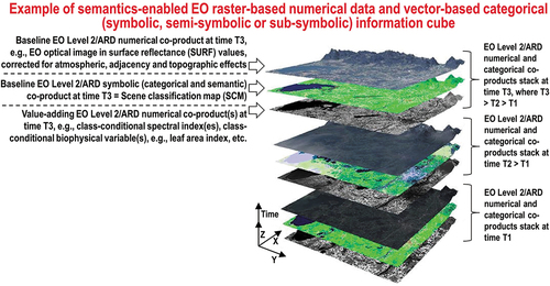
Due to lack of semantics in the adopted ARD baseline, if any, existing EO big (raster-based) data cube implementations together with the five existing DIAS 1.0 instantiations are affected by the so-called DRIP syndrome (refer to references listed in Section 2). According to Section 2, existing EO big (raster-based) data cube management systems are affected by the DRIP syndrome because they are not provided with any integrated ‘AGI ⊃ CV ⊃ EO-IU ⊃ ARD’ component system in operational mode as inference engine, capable of transforming at the edge (Intelligent Edge Conference, 2021), as close as possible to the sensory data acquisition stage, either on-line or off-line, at the space segment (EOportal, 2020; ESA – European Space Agency, 2019; Esposito et al., 2019a, 2019b; Zhou, 2001) and/or midstream segment (NASA – National Aeronautics and Space Administration, 2019; CEOS – Committee on Earth Observation Satellites, 2018; DLR – Deutsches Zentrum für Luft-und Raumfahrt e.V. and VEGA Technologies, 2011; Dwyer et al., 2018; ESA – European Space Agency, 2015; Gómez-Chova et al., 2007; Helder et al., 2018; Houborga & McCabe, 2018; OHB, 2016; USGS – U.S. Geological Survey, 2018a, 2018b, 2018c; Vermote & Saleous, 2007) (see Figure 10), EO big sensory data, characterized by the six Vs of volume, variety, veracity, velocity, volatility and value (Metternicht et al., 2020), into EO data-derived Level 2/ARD raster-based numerical variable co-product(s) stacked with vector-based symbolic (categorical and semantic) information co-product(s) (Augustin et al., 2018, 2019; Baraldi et al., 2016, 2017; FFG – Austrian Research Promotion Agency, 2015, 2016, 2018, 2020; Sudmanns et al., 2018; Tiede et al., 2017) (refer to Subsection 3.3.1), in analogy with the semantics-enriched ESA Sentinel-2 Level 2 co-product pair available to date (DLR – Deutsches Zentrum für Luft-und Raumfahrt e.V. and VEGA Technologies, 2011; ESA – European Space Agency, 2015), consisting of one Sentinel-2 sensory data-derived radiometrically calibrated image (2D gridded data) stacked with its sensory data-derived SCM information product, see Figure 38.

Figure 40. Architecture (design) of a closed-loop artificial general intelligence (AGI) (Bills, 2020; Chollet, 2019; Dreyfus, 1965, 1991, 1992; EC – European Commission, 2019; Fjelland, 2020; Hassabis et al., 2017; Ideami, 2021; Jajal, 2018; Jordan, 2018; Mindfire Foundation, 2018; Practical AI, 2020; Romero, 2021; Santoro et al., 2021; Sweeney, 2018a; Wolski, 2020a, 2020b) for Data and Information Access Services (AGI4DIAS) = Equation (1)(1) $\begin{array}{rl}& \text{lsquo}\mathrm{A}\mathrm{G}\mathrm{I}\text{-}\mathrm{e}\mathrm{n}\mathrm{a}\mathrm{b}\mathrm{l}\mathrm{e}\mathrm{d}\mathrm{D}\mathrm{I}\mathrm{A}\mathrm{S}=\mathrm{A}\mathrm{G}\mathrm{I}4\mathrm{D}\mathrm{I}\mathrm{A}\mathrm{S}=\mathrm{S}\mathrm{e}\mathrm{m}\mathrm{a}\mathrm{n}\mathrm{t}\mathrm{i}\mathrm{c}\mathrm{s}\text{-}\mathrm{e}\mathrm{n}\mathrm{a}\mathrm{b}\mathrm{l}\mathrm{e}\mathrm{d}\mathrm{D}\mathrm{I}\mathrm{A}\mathrm{S}2.0\\ & (\mathrm{D}\mathrm{I}\mathrm{A}\mathrm{S}{2}^{\mathrm{n}\mathrm{d}}\mathrm{g}\mathrm{e}\mathrm{n}\mathrm{e}\mathrm{r}\mathrm{a}\mathrm{t}\mathrm{i}\mathrm{o}\mathrm{n})=\mathrm{D}\mathrm{I}\mathrm{A}\mathrm{S}2.0=\mathrm{A}\mathrm{G}\mathrm{I}+\mathrm{D}\mathrm{I}\mathrm{A}\mathrm{S}1.0+\mathrm{S}\mathrm{C}\mathrm{B}\mathrm{I}\mathrm{R}+\mathrm{S}\mathrm{E}\mathrm{I}\mathrm{K}\mathrm{D}\text{rsquo}\end{array}$(1) , synonym for semantics-enabled EO big raster-based (numerical) data and vector-based categorical (either subsymbolic, semi-symbolic or symbolic) information cube management system (Augustin et al., 2018, 2019; Baraldi et al., 2016, 2017; FFG – Austrian Research Promotion Agency, 2015, 2016, 2018, 2020; Sudmanns et al., 2021; Sudmanns et al., 2018; Tiede et al., 2017) (see Figure 39), capable of incremental (semantic) learning. AGI4DIAS is considered necessary-but-not-sufficient precondition to semantic content-based image retrieval (SCBIR) and semantics-enabled information/knowledge discovery (SEIKD) over heterogeneous data sources acquired through geospace-time and imaging sensors, where SCBIR and SEIKD are consistent with symbolic human reasoning in human-speak (Augustin et al., 2018, 2019; Baraldi, 2017; Baraldi & Tiede, 2018a, 2018b; Baraldi et al., 2016, 2017; Dhurba & King, 2005; Newell & Simon, 1972; Planet, 2018; Sudmanns et al., 2021; Sudmanns et al., 2018; Tiede et al., 2017), also refer to Figure 2 and Figure 10. The AGI4DIAS system architecture (design) consists of a feedback hybrid ‘ARD ⊂ EO-IU ⊂ CV ⊂ AGI’ = Equation (3)(3) $\text{lsquo}\mathrm{A}\mathrm{R}\mathrm{D}\subset \mathrm{E}\mathrm{O}-\mathrm{I}\mathrm{U}\subset \mathrm{C}\mathrm{V}\subset \mathrm{A}\mathrm{G}\mathrm{I}\subset \mathrm{C}\mathrm{o}\mathrm{g}\mathrm{n}\mathrm{i}\mathrm{t}\mathrm{i}\mathrm{v}\mathrm{e}\mathrm{s}\mathrm{c}\mathrm{i}\mathrm{e}\mathrm{n}\mathrm{c}\mathrm{e}\text{rsquo}$(3) subsystem (see Figure 34) in closed-loop with an EO Semantic Querying (SQ) subsystem. The hybrid feedback ‘ARD ⊂ EO-IU ⊂ CV ⊂ AGI’ = Equation (3)(3) $\text{lsquo}\mathrm{A}\mathrm{R}\mathrm{D}\subset \mathrm{E}\mathrm{O}-\mathrm{I}\mathrm{U}\subset \mathrm{C}\mathrm{V}\subset \mathrm{A}\mathrm{G}\mathrm{I}\subset \mathrm{C}\mathrm{o}\mathrm{g}\mathrm{n}\mathrm{i}\mathrm{t}\mathrm{i}\mathrm{v}\mathrm{e}\mathrm{s}\mathrm{c}\mathrm{i}\mathrm{e}\mathrm{n}\mathrm{c}\mathrm{e}\text{rsquo}$(3) component system (see Figure 34) is required to be in operational mode, automatic (no human-machine interaction is required by the EO-IU subsystem to run) and near real-time, to provide the EO-SQ subsystem with value-adding EO sensory data-derived information products, including a Scene Classification Map (SCM), considered necessary-but-not-sufficient pre-condition to SQ, encompassing SCBIR and SEIKD operations in massive multi-source EO image bases. The EO-SQ subsystem is provided with a graphic user interface (GUI), to streamline: (i) top-down knowledge transfer, from-human-to-machine, of an a priori conceptual (mental) model of the 4D spatial-temporal real-world, (ii) high-level user- and application-specific SCBIR and SEIKD queries. Output products generated by the closed-loop AGI4DIAS system are expected to monotonically increase their value-added informativeness with closed-loop iterations, according to Bayesian updating, where Bayesian inference is applied iteratively: after observing some evidence, the resulting posterior probability can be treated as a prior probability and a new posterior probability computed from new evidence (Bowers & Davis, 2012; Ghahramani, 2011; Lähteenlahti, 2021; Sarkar, 2018).

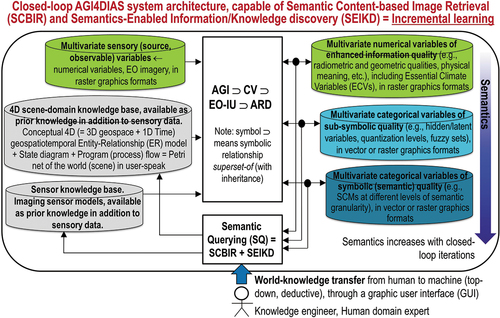
The notion of semantics-enabled EO big raster-based numerical data and vector-based categorical (symbolic, semi-symbolic or subsymbolic) information cube management system, requiring an integrated ‘AGI ⊃ CV ⊃ EO-IU ⊃ ARD’ capability at the edge (Intelligent Edge Conference, 2021), suitable for EO big raster-based numerical data interpretation into vector-based semantics (refer to Subsection 3.3.1), occurring as close as possible to the spaceborne/airborne EO imaging sensor, either on-line or off-line, at the space segment and/or midstream segment (see Figure 10), complies with, first, the seminal intuition by Marr quoted in Section 2 (Marr, 1982, p. 343).

Second, it agrees with the notion of future intelligent EO satellites dating back to the late ‘90s (Zhou, 2001). Future developments in AGI applications at the space segment (AGI4Space) (EOportal, 2020; ESA – European Space Agency, 2019; Esposito et al., 2019a, 2019b; GISCafe News, 2018; Zhou, 2001) (see Figure 10) are envisioned by the following quote (GISCafe News, 2018): “The Earth-i led consortium will develop a number of new Earth Observation technologies that will enable processes, such as the enhancement of image resolution, cloud-detection, change detection and video compression, to take place on-board a small satellite rather than on the ground. This will accelerate the delivery of high-quality images, video and information-rich analytics to end-users. On-board cloud detection will make the tasking of satellites more efficient and increase the probability of capturing a usable and useful image or video. To achieve these goals, ‘Project OVERPaSS‘ will implement, test and demonstrate very high-resolution optical image analysis techniques, involving both new software and dedicated hardware installed onboard small satellites to radically increase their ability to process data in space. The project will also determine the extent to which these capabilities could be routinely deployed on-board British optical imaging satellites in the future.”

Figure 41. In agreement with symbols adopted by the standard Unified Modeling Language (UML) for graphical modeling of object-oriented software (Fowler, 2003), relationship part-of, denoted with symbol ‘→’ pointing from the supplier to the client, should not to be confused with relationship subset-of, ‘⊃’, meaning specialization with inheritance from the superset (at left) to the subset. A National Aeronautics and Space Administration (NASA) EO (e.g. Landsat-8) Level 2 product is defined as “a data-derived geophysical variable at the same resolution and location as Level 1 source data” (NASA, 2018). Herein, subsymbolic NASA EO Level 2 is considered part-of a semantics-enriched ESA EO (e.g. Sentinel-2) sensory image-derived Level 2/Analysis Ready Data (ARD) co-product pair, defined as (DLR – Deutsches Zentrum für Luft-und Raumfahrt e.V. and VEGA Technologies, 2011; ESA – European Space Agency, 2015): (a) a single-date multi-spectral (MS) image whose digital numbers (DNs) are radiometrically calibrated into surface reflectance (SURF) 3-of-3 values (refer to Subsection 3.3.2), corrected in sequence for atmospheric effects (into SURF 1-of-3 values), topographic effects (into SURF 2-of-3 values) and adjacency effects (into SURF 3-of-3 values) (Egorov, Roy, Zhang, Hansen, and Kommareddy, 2018), stacked with (b) its data-derived general-purpose, user- and application-independent Scene Classification Map (SCM), whose thematic map legend includes quality layers Cloud and Cloud–shadow. A semantics-enriched ESA EO Level 2 co-product pair is regarded as an information primitive (unit of information) to be accomplished by Artificial General Intelligence for the Space segment (AGI4Space), such as in future intelligent small satellite constellations (EOportal, 2020; ESA – European Space Agency, 2019; Esposito et al., 2019a, 2019b; GISCafe News, 2018; Zhou, 2001), and/or at the midstream segment in an AGI for Data and Information Access Services (AGI4DIAS) framework, see Figure 10. In the graphical representation shown above, additional acronyms of interest are computer vision (CV), whose special case is EO image understanding (EO-IU) in operational mode, semantic content-based image retrieval (SCBIR), semantics-enabled information/knowledge discovery (SEIKD), where SCBIR + SEIKD is considered synonym for AGI4DIAS (see Figure 10), and Global Earth Observation System of (component) Systems (GEOSS), defined by the Group on Earth Observations (GEO) (EC – European Commission and GEO – Group on Earth Observations, 2014; GEO – Group on Earth Observations, 2005, 2019; Mavridis, 2011) and revised by GEO for years 2016–2025 as a new expert EO data-derived information and knowledge system (GEO – Group on Earth Observations, 2015; Nativi et al., 2015, 2020; Santoro et al., 2017), see Figure 1. Proposed in (Baraldi, 2017; Baraldi & Tiede, 2018a, 2018b), this working hypothesis postulates that GEOSS, whose parts-of are the still-unsolved (open) problems of SCBIR and SEIKD, cannot be achieved until the necessary-but-not-sufficient precondition of CV in operational mode, specifically, systematic semantics-enriched ESA-like EO image-derived Level 2 co-product pair generation, is accomplished in advance. If the aforementioned working hypothesis holds true, then the complexity of SCBIR and SEIKD is not inferior to the complexity of vision, acknowledged to be inherently ill-posed in the Hadamard sense (Hadamard, 1902) and non-deterministic polynomial (NP)-hard in computational complexity (Baraldi, 2017; Baraldi et al., 2018a, 2018b; Baraldi & Tiede, 2018a, 2018b; Frintrop, 2011; Matsuyama & Hwang, 1990; Tsotsos, 1990), see Figure 20. In other words, SCBIR, SEIKD and CV are all AGI-complete problems (Saba, 2020c; Wikipedia, 2021a) (refer to Section2). To make the inherently-ill-posed CV problem better conditioned for numerical solution (Baraldi, 2017; Bishop, 1995; Cherkassky & Mulier, 1998; Dubey et al., 2018), a CV system is constrained to include (as part-of) a computational model of human vision (Baraldi, 2017; Baraldi et al., 2018a, 2018b; Baraldi & Tiede, 2018a, 2018b; Iqbal & Aggarwal, 2001), i.e. Equation (4)(4) $\begin{array}{rl}& \text{lsquo}(Inductive/bottom\text{-}up/statisticalmodel\text{-}based)DL\text{-}from\text{-}data\subset \\ & (Inductive/bottom\text{-}up/statisticalmodel\text{-}based)ML\text{-}from\text{-}data\\ & \to AGI\supset CV\leftarrow Humanvision\text{rsquo}\end{array}$(4) = ‘Human vision → CV’ holds (see Figure 11), in agreement with a reverse engineering approach to CV (Bharath & Petrou, 2008; DiCarlo, 2017), see Figure 26.

Third, it agrees with the GEO second implementation plan for years 2016–2025 of a new GEOSS, regarded as expert EO data-derived information and knowledge system (GEO – Group on Earth Observations, 2015; Nativi et al., 2015, 2020; Santoro et al., 2017) (see Figure 1), in agreement with the increasingly popular DIKW conceptual hierarchy (Rowley, 2007; Rowley & Hartley, 2008; Wikipedia, 2020a; Zeleny, 1987, 2005; Zins, 2007), see Figure 12 and Figure 16.

In Section 2, starting from a traditional EC-DIAS 1.0 infrastructure (EU – European Union, 2017, 2018), affected by the DRIP syndrome because provided with no ‘AGI ⊃ CV ⊃ EO-IU’ subsystem in operational mode, an integrated AGI-enabled DIAS infrastructure = ‘AGI4DIAS = DIAS 2.0 = DIAS 1.0 + AGI + SCBIR + SEIKD’ = Equation (1)(1) $\begin{array}{rl}& \text{lsquo}\mathrm{A}\mathrm{G}\mathrm{I}\text{-}\mathrm{e}\mathrm{n}\mathrm{a}\mathrm{b}\mathrm{l}\mathrm{e}\mathrm{d}\mathrm{D}\mathrm{I}\mathrm{A}\mathrm{S}=\mathrm{A}\mathrm{G}\mathrm{I}4\mathrm{D}\mathrm{I}\mathrm{A}\mathrm{S}=\mathrm{S}\mathrm{e}\mathrm{m}\mathrm{a}\mathrm{n}\mathrm{t}\mathrm{i}\mathrm{c}\mathrm{s}\text{-}\mathrm{e}\mathrm{n}\mathrm{a}\mathrm{b}\mathrm{l}\mathrm{e}\mathrm{d}\mathrm{D}\mathrm{I}\mathrm{A}\mathrm{S}2.0\\ & (\mathrm{D}\mathrm{I}\mathrm{A}\mathrm{S}{2}^{\mathrm{n}\mathrm{d}}\mathrm{g}\mathrm{e}\mathrm{n}\mathrm{e}\mathrm{r}\mathrm{a}\mathrm{t}\mathrm{i}\mathrm{o}\mathrm{n})=\mathrm{D}\mathrm{I}\mathrm{A}\mathrm{S}2.0=\mathrm{A}\mathrm{G}\mathrm{I}+\mathrm{D}\mathrm{I}\mathrm{A}\mathrm{S}1.0+\mathrm{S}\mathrm{C}\mathrm{B}\mathrm{I}\mathrm{R}+\mathrm{S}\mathrm{E}\mathrm{I}\mathrm{K}\mathrm{D}\text{rsquo}\end{array}$(1) is proposed for implementation at the midstream segment, see Figure 2 and Figure 10. In agreement with a new notion of AGI4DIAS infrastructure = Equation (1)(1) $\begin{array}{rl}& \text{lsquo}\mathrm{A}\mathrm{G}\mathrm{I}\text{-}\mathrm{e}\mathrm{n}\mathrm{a}\mathrm{b}\mathrm{l}\mathrm{e}\mathrm{d}\mathrm{D}\mathrm{I}\mathrm{A}\mathrm{S}=\mathrm{A}\mathrm{G}\mathrm{I}4\mathrm{D}\mathrm{I}\mathrm{A}\mathrm{S}=\mathrm{S}\mathrm{e}\mathrm{m}\mathrm{a}\mathrm{n}\mathrm{t}\mathrm{i}\mathrm{c}\mathrm{s}\text{-}\mathrm{e}\mathrm{n}\mathrm{a}\mathrm{b}\mathrm{l}\mathrm{e}\mathrm{d}\mathrm{D}\mathrm{I}\mathrm{A}\mathrm{S}2.0\\ & (\mathrm{D}\mathrm{I}\mathrm{A}\mathrm{S}{2}^{\mathrm{n}\mathrm{d}}\mathrm{g}\mathrm{e}\mathrm{n}\mathrm{e}\mathrm{r}\mathrm{a}\mathrm{t}\mathrm{i}\mathrm{o}\mathrm{n})=\mathrm{D}\mathrm{I}\mathrm{A}\mathrm{S}2.0=\mathrm{A}\mathrm{G}\mathrm{I}+\mathrm{D}\mathrm{I}\mathrm{A}\mathrm{S}1.0+\mathrm{S}\mathrm{C}\mathrm{B}\mathrm{I}\mathrm{R}+\mathrm{S}\mathrm{E}\mathrm{I}\mathrm{K}\mathrm{D}\text{rsquo}\end{array}$(1) to be implemented at the midstream segment, a semantics-enabled EO big raster-based numerical data and vector-based categorical information cube management system is regarded as necessary-but-not-sufficient precondition to SCBIR and SEIKD activities, conducted over heterogeneous data sources acquired across geospace-time and EO imaging sensors, envisioned by portions of the existing literature (refer to references listed in Section 2), see Figure 41.

In general, SCBIR and SEIKD solutions are intuitive to deal with, i.e. they are easy to use, because consistent with symbolic human reasoning in natural language (Baraldi, 2017; Green et al., 2002; Kuhn, 2005; Laurini & Thompson, 1992; Matsuyama & Hwang, 1990; Newell & Simon, 1972; Sheth, 2015; Sonka et al., 1994; Sowa, 2000). If EO image-derived ARD-specific SCMs are generated systematically through geospace-time and EO imaging sensors, then an AGI4DIAS = Equation (1)(1) $\begin{array}{rl}& \text{lsquo}\mathrm{A}\mathrm{G}\mathrm{I}\text{-}\mathrm{e}\mathrm{n}\mathrm{a}\mathrm{b}\mathrm{l}\mathrm{e}\mathrm{d}\mathrm{D}\mathrm{I}\mathrm{A}\mathrm{S}=\mathrm{A}\mathrm{G}\mathrm{I}4\mathrm{D}\mathrm{I}\mathrm{A}\mathrm{S}=\mathrm{S}\mathrm{e}\mathrm{m}\mathrm{a}\mathrm{n}\mathrm{t}\mathrm{i}\mathrm{c}\mathrm{s}\text{-}\mathrm{e}\mathrm{n}\mathrm{a}\mathrm{b}\mathrm{l}\mathrm{e}\mathrm{d}\mathrm{D}\mathrm{I}\mathrm{A}\mathrm{S}2.0\\ & (\mathrm{D}\mathrm{I}\mathrm{A}\mathrm{S}{2}^{\mathrm{n}\mathrm{d}}\mathrm{g}\mathrm{e}\mathrm{n}\mathrm{e}\mathrm{r}\mathrm{a}\mathrm{t}\mathrm{i}\mathrm{o}\mathrm{n})=\mathrm{D}\mathrm{I}\mathrm{A}\mathrm{S}2.0=\mathrm{A}\mathrm{G}\mathrm{I}+\mathrm{D}\mathrm{I}\mathrm{A}\mathrm{S}1.0+\mathrm{S}\mathrm{C}\mathrm{B}\mathrm{I}\mathrm{R}+\mathrm{S}\mathrm{E}\mathrm{I}\mathrm{K}\mathrm{D}\text{rsquo}\end{array}$(1) infrastructure, consisting of a semantics-enabled EO big raster-based data and vector-based categorical information cube management system (see Figure 41), provided with SCBIR and SEIKD capabilities, would become a viable alternative to existing EO metadata text-based image retrieval systems in operational mode (Airbus, 2018; Planet, 2017). Capable of subsymbolic image querying by metadata text information (e.g. EO image acquisition time, geographic area of interest, etc.), including image-wide summary statistics (e.g. per-image cloud cover quality index), existing metadata text-based image retrieval capabilities are included, as part-of (without inheritance), in CBIR system prototypes, whose typical architecture is shown in Figure 4. Also known as Query by Image Content (QBIC) (Tyagi, 2017), prototypical implementations of CBIR systems take an image, image-object or multi-object examples as query and return from the image database a ranked set of images similar in content to the query (Datta et al., 2008; Kumar et al., 2011; Ma & Manjunath, 1997; Shyu et al., 2007; Smeulders et al., 2000; Smith & Chang, 1996; Tyagi, 2017).

Unfortunately, existing EO-CBIR system prototypes feature no semantic querying capability in user-speak (natural language) (Brinkworth, 1992), required to process semantic queries such as “retrieve all EO images not necessarily cloud-free acquired by imaging sensor X where wetland areas are visible and located adjacent to a highway near a coast in the eastern part of country Y” (Dhurba & King, 2005). The same lack of geospatio-temporal “intelligence” affects the so-called SCBIR system proposed by Wang et al., where MS images are classified off-line and then retrieved based on an image-wide semantic histogram-pair (spatial topology non-preserving bag-of-visual-words) similarity index between a query image and each candidate image stored in the database (Wang, Wan, Gu, & Song, 2013). It means that the so-called SCBIR system presented in (Wang et al., 2013) does not satisfy the aforementioned definition of SCBIR system, adopted herein in agreement with the work by Dhurba and King (Dhurba & King, 2005), where SCBIR requires the same capabilities in geospatio-temporal reasoning (geospace-time intelligence) featured by existing geographic information systems (Couclelis, 2012), see Figure 11. In the GISscience domain, traditional geographic information systems support geospatio-temporal reasoning on information primitives, pertaining to a (2D) image-plane, of three types: geo-object (geospatial categorical/ nominal/ qualitative variable of symbolic quality), geo-field (geospatial numerical/quantitative variable of subsymbolic quality) and field-object (geospatial numerical variable obtained from geo-field discretization) (Couclelis, 2010; Goodchild et al., 2007) (refer to Subsection 3.3.1).

Originally proposed in (Baraldi, 2017; Baraldi & Tiede, 2018a, 2018b), the working hypothesis shown in Figure 41 postulates that the following dependence relationship holds true:

(13) $\begin{array}{rl}& \text{lsquo}\mathrm{N}\mathrm{A}\mathrm{S}\mathrm{A}\mathrm{E}\mathrm{O}\left(\mathrm{e}.\mathrm{g}.,\mathrm{L}\mathrm{a}\mathrm{n}\mathrm{d}\mathrm{s}\mathrm{a}\mathrm{t}\text{-}8\right)\mathrm{L}\mathrm{e}\mathrm{v}\mathrm{e}\mathrm{l}2\left(\mathrm{n}\mathrm{u}\mathrm{m}\mathrm{e}\mathrm{r}\mathrm{i}\mathrm{c}\mathrm{a}\mathrm{l},\mathrm{s}\mathrm{u}\mathrm{b}\text{-}\mathrm{s}\mathrm{y}\mathrm{m}\mathrm{b}\mathrm{o}\mathrm{l}\mathrm{i}\mathrm{c}\right)\\ & \mathrm{p}\mathrm{r}\mathrm{o}\mathrm{d}\mathrm{u}\mathrm{c}\mathrm{t}\to \mathrm{S}\mathrm{e}\mathrm{m}\mathrm{a}\mathrm{n}\mathrm{t}\mathrm{i}\mathrm{c}\mathrm{s}\text{-}\mathrm{e}\mathrm{n}\mathrm{r}\mathrm{i}\mathrm{c}\mathrm{h}\mathrm{e}\mathrm{d}\mathrm{E}\mathrm{S}\mathrm{A}\text{-}\mathrm{l}\mathrm{i}\mathrm{k}\mathrm{e}\left(\mathrm{e}.\mathrm{g}.,\mathrm{S}\mathrm{e}\mathrm{n}\mathrm{t}\mathrm{i}\mathrm{n}\mathrm{e}\mathrm{l}\text{-}2\right)\\ & \mathrm{E}\mathrm{O}\mathrm{L}\mathrm{e}\mathrm{v}\mathrm{e}\mathrm{l}2/\mathrm{A}\mathrm{R}\mathrm{D}\mathrm{c}\mathrm{o}\text{-}\mathrm{p}\mathrm{r}\mathrm{o}\mathrm{d}\mathrm{u}\mathrm{c}\mathrm{t}\mathrm{p}\mathrm{a}\mathrm{i}\mathrm{r},\mathrm{e}\mathrm{x}\mathrm{p}\mathrm{e}\mathrm{c}\mathrm{t}\mathrm{e}\mathrm{d}\mathrm{t}\mathrm{o}\mathrm{b}\mathrm{e}\mathrm{s}\mathrm{o}\mathrm{l}\mathrm{v}\mathrm{e}\mathrm{d}\mathrm{a}\mathrm{t}\\ & \mathrm{t}\mathrm{h}\mathrm{e}\mathrm{s}\mathrm{p}\mathrm{a}\mathrm{c}\mathrm{e}\mathrm{s}\mathrm{e}\mathrm{g}\mathrm{m}\mathrm{e}\mathrm{n}\mathrm{t}\mathrm{a}\mathrm{s}\mathrm{A}\mathrm{G}\mathrm{I}4\mathrm{S}\mathrm{p}\mathrm{a}\mathrm{c}\mathrm{e}\subset \mathrm{E}\mathrm{O}\text{-}\mathrm{I}\mathrm{U}\mathrm{i}\mathrm{n}\mathrm{o}\mathrm{p}\mathrm{e}\mathrm{r}\mathrm{a}\mathrm{t}\mathrm{i}\mathrm{o}\mathrm{n}\mathrm{a}\mathrm{l}\mathrm{m}\mathrm{o}\mathrm{d}\mathrm{e}\\ & \subset \mathrm{C}\mathrm{V}\subset \mathrm{A}\mathrm{G}\mathrm{I}\to \left[\mathrm{E}\mathrm{O}\text{-}\mathrm{S}\mathrm{C}\mathrm{B}\mathrm{I}\mathrm{R}+\mathrm{S}\mathrm{E}\mathrm{I}\mathrm{K}\mathrm{D}=\mathrm{s}\mathrm{e}\mathrm{m}\mathrm{a}\mathrm{n}\mathrm{t}\mathrm{i}\mathrm{c}\mathrm{s}\text{-}\mathrm{e}\mathrm{n}\mathrm{a}\mathrm{b}\mathrm{l}\mathrm{e}\mathrm{d}\mathrm{A}\mathrm{G}\mathrm{I}4\mathrm{D}\mathrm{I}\mathrm{A}\mathrm{S}\right]\\ & \to \mathrm{G}\mathrm{E}\mathrm{O}\text{-}\mathrm{G}\mathrm{E}\mathrm{O}\mathrm{S}\mathrm{S}\text{rsquo}\end{array}$(13)

Equation (13)(13) $\begin{array}{rl}& \text{lsquo}\mathrm{N}\mathrm{A}\mathrm{S}\mathrm{A}\mathrm{E}\mathrm{O}\left(\mathrm{e}.\mathrm{g}.,\mathrm{L}\mathrm{a}\mathrm{n}\mathrm{d}\mathrm{s}\mathrm{a}\mathrm{t}\text{-}8\right)\mathrm{L}\mathrm{e}\mathrm{v}\mathrm{e}\mathrm{l}2\left(\mathrm{n}\mathrm{u}\mathrm{m}\mathrm{e}\mathrm{r}\mathrm{i}\mathrm{c}\mathrm{a}\mathrm{l},\mathrm{s}\mathrm{u}\mathrm{b}\text{-}\mathrm{s}\mathrm{y}\mathrm{m}\mathrm{b}\mathrm{o}\mathrm{l}\mathrm{i}\mathrm{c}\right)\\ & \mathrm{p}\mathrm{r}\mathrm{o}\mathrm{d}\mathrm{u}\mathrm{c}\mathrm{t}\to \mathrm{S}\mathrm{e}\mathrm{m}\mathrm{a}\mathrm{n}\mathrm{t}\mathrm{i}\mathrm{c}\mathrm{s}\text{-}\mathrm{e}\mathrm{n}\mathrm{r}\mathrm{i}\mathrm{c}\mathrm{h}\mathrm{e}\mathrm{d}\mathrm{E}\mathrm{S}\mathrm{A}\text{-}\mathrm{l}\mathrm{i}\mathrm{k}\mathrm{e}\left(\mathrm{e}.\mathrm{g}.,\mathrm{S}\mathrm{e}\mathrm{n}\mathrm{t}\mathrm{i}\mathrm{n}\mathrm{e}\mathrm{l}\text{-}2\right)\\ & \mathrm{E}\mathrm{O}\mathrm{L}\mathrm{e}\mathrm{v}\mathrm{e}\mathrm{l}2/\mathrm{A}\mathrm{R}\mathrm{D}\mathrm{c}\mathrm{o}\text{-}\mathrm{p}\mathrm{r}\mathrm{o}\mathrm{d}\mathrm{u}\mathrm{c}\mathrm{t}\mathrm{p}\mathrm{a}\mathrm{i}\mathrm{r},\mathrm{e}\mathrm{x}\mathrm{p}\mathrm{e}\mathrm{c}\mathrm{t}\mathrm{e}\mathrm{d}\mathrm{t}\mathrm{o}\mathrm{b}\mathrm{e}\mathrm{s}\mathrm{o}\mathrm{l}\mathrm{v}\mathrm{e}\mathrm{d}\mathrm{a}\mathrm{t}\\ & \mathrm{t}\mathrm{h}\mathrm{e}\mathrm{s}\mathrm{p}\mathrm{a}\mathrm{c}\mathrm{e}\mathrm{s}\mathrm{e}\mathrm{g}\mathrm{m}\mathrm{e}\mathrm{n}\mathrm{t}\mathrm{a}\mathrm{s}\mathrm{A}\mathrm{G}\mathrm{I}4\mathrm{S}\mathrm{p}\mathrm{a}\mathrm{c}\mathrm{e}\subset \mathrm{E}\mathrm{O}\text{-}\mathrm{I}\mathrm{U}\mathrm{i}\mathrm{n}\mathrm{o}\mathrm{p}\mathrm{e}\mathrm{r}\mathrm{a}\mathrm{t}\mathrm{i}\mathrm{o}\mathrm{n}\mathrm{a}\mathrm{l}\mathrm{m}\mathrm{o}\mathrm{d}\mathrm{e}\\ & \subset \mathrm{C}\mathrm{V}\subset \mathrm{A}\mathrm{G}\mathrm{I}\to \left[\mathrm{E}\mathrm{O}\text{-}\mathrm{S}\mathrm{C}\mathrm{B}\mathrm{I}\mathrm{R}+\mathrm{S}\mathrm{E}\mathrm{I}\mathrm{K}\mathrm{D}=\mathrm{s}\mathrm{e}\mathrm{m}\mathrm{a}\mathrm{n}\mathrm{t}\mathrm{i}\mathrm{c}\mathrm{s}\text{-}\mathrm{e}\mathrm{n}\mathrm{a}\mathrm{b}\mathrm{l}\mathrm{e}\mathrm{d}\mathrm{A}\mathrm{G}\mathrm{I}4\mathrm{D}\mathrm{I}\mathrm{A}\mathrm{S}\right]\\ & \to \mathrm{G}\mathrm{E}\mathrm{O}\text{-}\mathrm{G}\mathrm{E}\mathrm{O}\mathrm{S}\mathrm{S}\text{rsquo}\end{array}$(13) means that the GEO visionary goal of a GEOSS (see Figure 1), to be considered an AGI-complete problem (Saba, 2020c; Wikipedia, 2021a) unaccomplished to date (GEO – Group on Earth Observations, 2015; Nativi et al., 2015, 2020), whose parts-of are the still-unsolved (open) AGI-complete problems of SCBIR and SEIKD (Saba, 2020c; Wikipedia, 2021a), cannot be achieved until the necessary-but-not-sufficient precondition of ‘AGI ⊃ CV ⊃ EO-IU ⊃ ARD’ = Equation (3)(3) $\text{lsquo}\mathrm{A}\mathrm{R}\mathrm{D}\subset \mathrm{E}\mathrm{O}-\mathrm{I}\mathrm{U}\subset \mathrm{C}\mathrm{V}\subset \mathrm{A}\mathrm{G}\mathrm{I}\subset \mathrm{C}\mathrm{o}\mathrm{g}\mathrm{n}\mathrm{i}\mathrm{t}\mathrm{i}\mathrm{v}\mathrm{e}\mathrm{s}\mathrm{c}\mathrm{i}\mathrm{e}\mathrm{n}\mathrm{c}\mathrm{e}\text{rsquo}$(3) , specifically, systematic multi-source semantics-enriched ESA-like EO (e.g. Sentinel-2) Level 2/ARD co-product pair generation (see Figure 35), to be considered an AGI-complete open problem to date, is accomplished in advance in operational mode (refer to Subsection 3.1). Intuitively, if Equation (13)(13) $\begin{array}{rl}& \text{lsquo}\mathrm{N}\mathrm{A}\mathrm{S}\mathrm{A}\mathrm{E}\mathrm{O}\left(\mathrm{e}.\mathrm{g}.,\mathrm{L}\mathrm{a}\mathrm{n}\mathrm{d}\mathrm{s}\mathrm{a}\mathrm{t}\text{-}8\right)\mathrm{L}\mathrm{e}\mathrm{v}\mathrm{e}\mathrm{l}2\left(\mathrm{n}\mathrm{u}\mathrm{m}\mathrm{e}\mathrm{r}\mathrm{i}\mathrm{c}\mathrm{a}\mathrm{l},\mathrm{s}\mathrm{u}\mathrm{b}\text{-}\mathrm{s}\mathrm{y}\mathrm{m}\mathrm{b}\mathrm{o}\mathrm{l}\mathrm{i}\mathrm{c}\right)\\ & \mathrm{p}\mathrm{r}\mathrm{o}\mathrm{d}\mathrm{u}\mathrm{c}\mathrm{t}\to \mathrm{S}\mathrm{e}\mathrm{m}\mathrm{a}\mathrm{n}\mathrm{t}\mathrm{i}\mathrm{c}\mathrm{s}\text{-}\mathrm{e}\mathrm{n}\mathrm{r}\mathrm{i}\mathrm{c}\mathrm{h}\mathrm{e}\mathrm{d}\mathrm{E}\mathrm{S}\mathrm{A}\text{-}\mathrm{l}\mathrm{i}\mathrm{k}\mathrm{e}\left(\mathrm{e}.\mathrm{g}.,\mathrm{S}\mathrm{e}\mathrm{n}\mathrm{t}\mathrm{i}\mathrm{n}\mathrm{e}\mathrm{l}\text{-}2\right)\\ & \mathrm{E}\mathrm{O}\mathrm{L}\mathrm{e}\mathrm{v}\mathrm{e}\mathrm{l}2/\mathrm{A}\mathrm{R}\mathrm{D}\mathrm{c}\mathrm{o}\text{-}\mathrm{p}\mathrm{r}\mathrm{o}\mathrm{d}\mathrm{u}\mathrm{c}\mathrm{t}\mathrm{p}\mathrm{a}\mathrm{i}\mathrm{r},\mathrm{e}\mathrm{x}\mathrm{p}\mathrm{e}\mathrm{c}\mathrm{t}\mathrm{e}\mathrm{d}\mathrm{t}\mathrm{o}\mathrm{b}\mathrm{e}\mathrm{s}\mathrm{o}\mathrm{l}\mathrm{v}\mathrm{e}\mathrm{d}\mathrm{a}\mathrm{t}\\ & \mathrm{t}\mathrm{h}\mathrm{e}\mathrm{s}\mathrm{p}\mathrm{a}\mathrm{c}\mathrm{e}\mathrm{s}\mathrm{e}\mathrm{g}\mathrm{m}\mathrm{e}\mathrm{n}\mathrm{t}\mathrm{a}\mathrm{s}\mathrm{A}\mathrm{G}\mathrm{I}4\mathrm{S}\mathrm{p}\mathrm{a}\mathrm{c}\mathrm{e}\subset \mathrm{E}\mathrm{O}\text{-}\mathrm{I}\mathrm{U}\mathrm{i}\mathrm{n}\mathrm{o}\mathrm{p}\mathrm{e}\mathrm{r}\mathrm{a}\mathrm{t}\mathrm{i}\mathrm{o}\mathrm{n}\mathrm{a}\mathrm{l}\mathrm{m}\mathrm{o}\mathrm{d}\mathrm{e}\\ & \subset \mathrm{C}\mathrm{V}\subset \mathrm{A}\mathrm{G}\mathrm{I}\to \left[\mathrm{E}\mathrm{O}\text{-}\mathrm{S}\mathrm{C}\mathrm{B}\mathrm{I}\mathrm{R}+\mathrm{S}\mathrm{E}\mathrm{I}\mathrm{K}\mathrm{D}=\mathrm{s}\mathrm{e}\mathrm{m}\mathrm{a}\mathrm{n}\mathrm{t}\mathrm{i}\mathrm{c}\mathrm{s}\text{-}\mathrm{e}\mathrm{n}\mathrm{a}\mathrm{b}\mathrm{l}\mathrm{e}\mathrm{d}\mathrm{A}\mathrm{G}\mathrm{I}4\mathrm{D}\mathrm{I}\mathrm{A}\mathrm{S}\right]\\ & \to \mathrm{G}\mathrm{E}\mathrm{O}\text{-}\mathrm{G}\mathrm{E}\mathrm{O}\mathrm{S}\mathrm{S}\text{rsquo}\end{array}$(13) holds true as working hypothesis, then the complexity of GEOSS, SCBIR, SEIKD and ARD is not inferior to the complexity of vision (see Figure 20), encompassing both biological vision and CV, acknowledged to be an AGI-complete problem (Saba, 2020c; Wikipedia, 2021a), which is inherently ill-posed in the Hadamard sense (Hadamard, 1902) and NP-hard in computational complexity (refer to Subsection 4.1). To make the inherently-ill-posed CV problem better conditioned for numerical solution (see Figure 20), our work requires a ‘CV ⊃ EO-IU ⊃ ARD’ system to comply with human visual perception, see Figure 11. In other words, a CV system is constrained to include (as part-of) a computational model of human vision, consistent with human visual perception phenomena (Baraldi, 2017; Baraldi et al., 2018a, 2018b; Iqbal & Aggarwal, 2001), such as visual illusions (Baraldi, 2017; Mély et al., 2018; Perez, 2018; Pessoa, 1996; Rappe, 2018) (refer to Subsection 4,2), i.e. semantic relationship ‘Human vision → CV’ = Equation (4)(4) $\begin{array}{rl}& \text{lsquo}(Inductive/bottom\text{-}up/statisticalmodel\text{-}based)DL\text{-}from\text{-}data\subset \\ & (Inductive/bottom\text{-}up/statisticalmodel\text{-}based)ML\text{-}from\text{-}data\\ & \to AGI\supset CV\leftarrow Humanvision\text{rsquo}\end{array}$(4) holds, in agreement with a reverse engineering approach to CV (Bharath & Petrou, 2008; DiCarlo, 2017), see Figure 26. Hence, dependence relationship:

(14) $\begin{array}{rl}& \text{lsquo}\mathrm{H}\mathrm{u}\mathrm{m}\mathrm{a}\mathrm{n}\mathrm{v}\mathrm{i}\mathrm{s}\mathrm{i}\mathrm{o}\mathrm{n}\to \mathrm{C}\mathrm{V}\supset \mathrm{E}\mathrm{O}\text{-}\mathrm{I}\mathrm{U}\mathrm{i}\mathrm{n}\mathrm{o}\mathrm{p}\mathrm{e}\mathrm{r}\mathrm{a}\mathrm{t}\mathrm{i}\mathrm{o}\mathrm{n}\mathrm{a}\mathrm{l}\mathrm{m}\mathrm{o}\mathrm{d}\mathrm{e}\supset \mathrm{N}\mathrm{A}\mathrm{S}\mathrm{A}\mathrm{E}\mathrm{O}\\ & \left(\mathrm{e}.\mathrm{g}.,\mathrm{L}\mathrm{a}\mathrm{n}\mathrm{d}\mathrm{s}\mathrm{a}\mathrm{t}\text{-}8\right)\mathrm{L}\mathrm{e}\mathrm{v}\mathrm{e}\mathrm{l}2\left(\mathrm{n}\mathrm{u}\mathrm{m}\mathrm{e}\mathrm{r}\mathrm{i}\mathrm{c}\mathrm{a}\mathrm{l},\mathrm{s}\mathrm{u}\mathrm{b}\text{-}\mathrm{s}\mathrm{y}\mathrm{m}\mathrm{b}\mathrm{o}\mathrm{l}\mathrm{i}\mathrm{c}\right)\\ & \mathrm{p}\mathrm{r}\mathrm{o}\mathrm{d}\mathrm{u}\mathrm{c}\mathrm{t}\to \mathrm{S}\mathrm{e}\mathrm{m}\mathrm{a}\mathrm{n}\mathrm{t}\mathrm{i}\mathrm{c}\mathrm{s}-\mathrm{e}\mathrm{n}\mathrm{r}\mathrm{i}\mathrm{c}\mathrm{h}\mathrm{e}\mathrm{d}\mathrm{E}\mathrm{S}\mathrm{A}\text{-}\mathrm{l}\mathrm{i}\mathrm{k}\mathrm{e}\mathrm{E}\mathrm{O}\left(\mathrm{e}.\mathrm{g}.,\mathrm{S}\mathrm{e}\mathrm{n}\mathrm{t}\mathrm{i}\mathrm{n}\mathrm{e}\mathrm{l}\text{-}2\right)\\ & \mathrm{L}\mathrm{e}\mathrm{v}\mathrm{e}\mathrm{l}2/\mathrm{A}\mathrm{R}\mathrm{D}\mathrm{c}\mathrm{o}\text{-}\mathrm{p}\mathrm{r}\mathrm{o}\mathrm{d}\mathrm{u}\mathrm{c}\mathrm{t}\mathrm{p}\mathrm{a}\mathrm{i}\mathrm{r}\to \\ & \left[\mathrm{E}\mathrm{O}\text{-}\mathrm{S}\mathrm{C}\mathrm{B}\mathrm{I}\mathrm{R}+\mathrm{S}\mathrm{E}\mathrm{I}\mathrm{K}\mathrm{D}=\mathrm{s}\mathrm{e}\mathrm{m}\mathrm{a}\mathrm{n}\mathrm{t}\mathrm{i}\mathrm{c}\mathrm{s}-\mathrm{e}\mathrm{n}\mathrm{a}\mathrm{b}\mathrm{l}\mathrm{e}\mathrm{d}\mathrm{A}\mathrm{G}\mathrm{I}4\mathrm{D}\mathrm{I}\mathrm{A}\mathrm{S}\right]\\ & \to \mathrm{G}\mathrm{E}\mathrm{O}\text{-}\mathrm{G}\mathrm{E}\mathrm{O}\mathrm{S}\mathrm{S}\leftarrow \mathrm{A}\mathrm{G}\mathrm{I}\subset \mathrm{C}\mathrm{o}\mathrm{g}\mathrm{n}\mathrm{i}\mathrm{t}\mathrm{i}\mathrm{v}\mathrm{e}\mathrm{s}\mathrm{c}\mathrm{i}\mathrm{e}\mathrm{n}\mathrm{c}\mathrm{e}\text{rsquo}\end{array}$(14)

holds as our working hypothesis, pertaining to the multi-disciplinary domain of cognitive science, see Figure 11. Equivalent to a first principle (axiom, postulate), Equation (14)(14) $\begin{array}{rl}& \text{lsquo}\mathrm{H}\mathrm{u}\mathrm{m}\mathrm{a}\mathrm{n}\mathrm{v}\mathrm{i}\mathrm{s}\mathrm{i}\mathrm{o}\mathrm{n}\to \mathrm{C}\mathrm{V}\supset \mathrm{E}\mathrm{O}\text{-}\mathrm{I}\mathrm{U}\mathrm{i}\mathrm{n}\mathrm{o}\mathrm{p}\mathrm{e}\mathrm{r}\mathrm{a}\mathrm{t}\mathrm{i}\mathrm{o}\mathrm{n}\mathrm{a}\mathrm{l}\mathrm{m}\mathrm{o}\mathrm{d}\mathrm{e}\supset \mathrm{N}\mathrm{A}\mathrm{S}\mathrm{A}\mathrm{E}\mathrm{O}\\ & \left(\mathrm{e}.\mathrm{g}.,\mathrm{L}\mathrm{a}\mathrm{n}\mathrm{d}\mathrm{s}\mathrm{a}\mathrm{t}\text{-}8\right)\mathrm{L}\mathrm{e}\mathrm{v}\mathrm{e}\mathrm{l}2\left(\mathrm{n}\mathrm{u}\mathrm{m}\mathrm{e}\mathrm{r}\mathrm{i}\mathrm{c}\mathrm{a}\mathrm{l},\mathrm{s}\mathrm{u}\mathrm{b}\text{-}\mathrm{s}\mathrm{y}\mathrm{m}\mathrm{b}\mathrm{o}\mathrm{l}\mathrm{i}\mathrm{c}\right)\\ & \mathrm{p}\mathrm{r}\mathrm{o}\mathrm{d}\mathrm{u}\mathrm{c}\mathrm{t}\to \mathrm{S}\mathrm{e}\mathrm{m}\mathrm{a}\mathrm{n}\mathrm{t}\mathrm{i}\mathrm{c}\mathrm{s}-\mathrm{e}\mathrm{n}\mathrm{r}\mathrm{i}\mathrm{c}\mathrm{h}\mathrm{e}\mathrm{d}\mathrm{E}\mathrm{S}\mathrm{A}\text{-}\mathrm{l}\mathrm{i}\mathrm{k}\mathrm{e}\mathrm{E}\mathrm{O}\left(\mathrm{e}.\mathrm{g}.,\mathrm{S}\mathrm{e}\mathrm{n}\mathrm{t}\mathrm{i}\mathrm{n}\mathrm{e}\mathrm{l}\text{-}2\right)\\ & \mathrm{L}\mathrm{e}\mathrm{v}\mathrm{e}\mathrm{l}2/\mathrm{A}\mathrm{R}\mathrm{D}\mathrm{c}\mathrm{o}\text{-}\mathrm{p}\mathrm{r}\mathrm{o}\mathrm{d}\mathrm{u}\mathrm{c}\mathrm{t}\mathrm{p}\mathrm{a}\mathrm{i}\mathrm{r}\to \\ & \left[\mathrm{E}\mathrm{O}\text{-}\mathrm{S}\mathrm{C}\mathrm{B}\mathrm{I}\mathrm{R}+\mathrm{S}\mathrm{E}\mathrm{I}\mathrm{K}\mathrm{D}=\mathrm{s}\mathrm{e}\mathrm{m}\mathrm{a}\mathrm{n}\mathrm{t}\mathrm{i}\mathrm{c}\mathrm{s}-\mathrm{e}\mathrm{n}\mathrm{a}\mathrm{b}\mathrm{l}\mathrm{e}\mathrm{d}\mathrm{A}\mathrm{G}\mathrm{I}4\mathrm{D}\mathrm{I}\mathrm{A}\mathrm{S}\right]\\ & \to \mathrm{G}\mathrm{E}\mathrm{O}\text{-}\mathrm{G}\mathrm{E}\mathrm{O}\mathrm{S}\mathrm{S}\leftarrow \mathrm{A}\mathrm{G}\mathrm{I}\subset \mathrm{C}\mathrm{o}\mathrm{g}\mathrm{n}\mathrm{i}\mathrm{t}\mathrm{i}\mathrm{v}\mathrm{e}\mathrm{s}\mathrm{c}\mathrm{i}\mathrm{e}\mathrm{n}\mathrm{c}\mathrm{e}\text{rsquo}\end{array}$(14) was considered the first original contribution, conceptual in nature, of the CV system proposed in (Baraldi, 2017; Baraldi & Tiede, 2018a, 2018b).

The observation that, among the existing four EO Level 2/ARD product definitions and four EO Level 2/ARD software implementations compared in Figures 35 and 36, only the ESA Sentinel-2 Level 2 product-pair definition and software implementation provide as output a symbolic (categorical and semantic) SCM co-product in addition to (stacked with) a numerical MS image of high scientific (quantitative) quality, because radiometrically calibrated into SURF 3-of-3 values, corrected (at least in theory) for atmospheric, topographic and adjacency effects (Egorov, Roy, Zhang, Hansen, and Kommareddy, 2018), deserves further discussion.

Figure 42. Example of automatic SIAM-based post-classification MS color naming change/no-change detection, starting from MS images acquired from different EO imaging sensors harmonized at the SIAM categorical level of color naming (see Figures 29 and 30), where SIAM stays for Satellite Image Automatic Mapper (SIAM) (Baraldi, 2017, 2019a; Baraldi et al., 2006, 2010a, 2010b, 2018a, 2018b; Baraldi & Tiede, 2018a, 2018b). Left: SIAM map depicted in 33 pseudo-colors, generated from a SPOT-5 image featuring four channels, specifically, visible green (G), visible red (R), near infrared (NIR) and middle infrared (MIR), radiometrically calibrated into TOARF values, upscaled to 5 m resolution. Center: SIAM map depicted in 33 pseudo-colors, generated from a RapidEye image featuring four channels, specifically, visible blue (B), G, R and NIR, radiometrically calibrated into TOARF values, 5 m resolution. Left: Multi-source SIAM-based post-classification change/no-change detection map, whose map legend consists of 29 codewords, depicted in pseudo-colors and associated with cells in a two-way 33 × 33 transition matrix with 33 entries as color names per date. The bi-temporal SIAM-based post-classification map legend is shown in Figures 43 and 44.

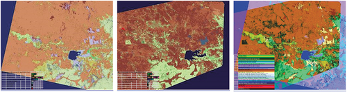
Lack of an output semantic co-product in ARD definitions and software implementations is quite surprising considering that, in the remaining three ARD product generation algorithms, namely, two USGS-NASA’s and one ASI’s, symbolic (categorical and semantic) Cloud/Not-Cloud = Rest-of-the-world layers/ strata/ masks (e.g. Water mask, Snow mask, Cloud-shadow mask, etc., in addition to the Cloud quality layer) are estimated and employed as ARD intermediate (hidden) products to correct Level 1 TOARF values from atmospheric effects into Level 2 SURF 1-of-3 values. Our claim is consistent with observations reported in the existing RS literature about radiometric Cal workflows, such as “classification is a prerequisite for the subsequent land cover-specific bidirectional reflectance distribution function (BRDF) correction” (Malenovsky et al., 2007), when SURF values are corrected into surface albedo values (Bilal et al., 2019; EC – European Commission, 2020; Egorov, Roy, Zhang, Hansen, and Kommareddy, 2018; Franch et al., 2019; Fuqin et al., 2012; Malenovsky et al., 2007; Qiu et al., 2019; Schaepman-Strub et al., 2006; Shuai et al., 2020) (refer to Subsection 3.3.2).

Lack of a symbolic (categorical and semantic) EO Level 2/ARD SCM co-product, although semantics was actually generated from EO data for internal ARD purposes (see Figure 35), reveals a serious misunderstanding by EO big data providers, including USGS-NASA and ASI, about what valuable information is to be inferred from EO sensory data to enable the downstream segment in the innovation chain required by a new Space Economy 4.0 (see Figure 10), where VAPS of incremental value are expected to be delivered at increasing levels of the processing chain. In agreement with the dual meaning of the concept of information discussed by philosophical hermeneutics (Capurro & Hjørland, 2003) (refer to Subsection 3.3.3), it is unquestionable that a symbolic (categorical and semantic) SCM co-product, pertaining to the qualitative/equivocal domain of information-as-data-interpretation, is complementary not-alternative to a numerical MS image radiometrically calibrated into ‘TOARF ⊇ SURF ⊇ surface albedo’ = Equation (8)(8) $\begin{array}{rl}& \text{lsquo}\mathrm{D}\mathrm{N}\mathrm{s}\ge 0\mathrm{a}\mathrm{t}\mathrm{E}\mathrm{O}\mathrm{L}\mathrm{e}\mathrm{v}\mathrm{e}\mathrm{l}0\supseteq \mathrm{T}\mathrm{O}\mathrm{A}\mathrm{R}\mathrm{F}\in \left[0.0,1.0\right]\mathrm{a}\mathrm{t}\mathrm{E}\mathrm{O}\mathrm{L}\mathrm{e}\mathrm{v}\mathrm{e}\mathrm{l}1\supseteq \mathrm{S}\mathrm{U}\mathrm{R}\mathrm{F}\in \left[0.0,1.0\right]\\ & \mathrm{a}\mathrm{t}\mathrm{E}\mathrm{O}\mathrm{L}\mathrm{e}\mathrm{v}\mathrm{e}\mathrm{l}2/\left(\mathrm{c}\mathrm{u}\mathrm{r}\mathrm{r}\mathrm{e}\mathrm{n}\mathrm{t}\right)\mathrm{A}\mathrm{R}\mathrm{D}\supseteq \mathrm{S}\mathrm{u}\mathrm{r}\mathrm{f}\mathrm{a}\mathrm{c}\mathrm{e}\mathrm{a}\mathrm{l}\mathrm{b}\mathrm{e}\mathrm{d}\mathrm{o}\in \left[0.0,1.0\right]\mathrm{a}\mathrm{t},\mathrm{s}\mathrm{a}\mathrm{y},\mathrm{E}\mathrm{O}\mathrm{L}\mathrm{e}\mathrm{v}\mathrm{e}\mathrm{l}3/\mathrm{n}\mathrm{e}\mathrm{x}\mathrm{t}\\ & \mathrm{g}\mathrm{e}\mathrm{n}\mathrm{e}\mathrm{r}\mathrm{a}\mathrm{t}\mathrm{i}\mathrm{o}\mathrm{n}\mathrm{A}\mathrm{R}\mathrm{D}\text{rsquo}& (8)\end{array}$(8) values, pertaining to the quantitative/unequivocal domain of information-as-thing.

These considerations comply with the observation that “[existing ARD do] not provide the information required by national agencies tasked with coordinating implementation of [the UN] SDGs. Instead, [national agencies] require standardised and informative end user products derived from ARD to track progress towards agreed targets. [Standardised and informative products required by end users include] land cover and its change over time, that contribute to the mapping and reporting on 14 of the 17 SDGs (GEO – Group on Earth Observations, 2020; Kavvada et al., 2020; Poussin et al., 2021). However, many nations lack access to an operational, standardised land cover product” (Owers et al., 2021) (refer to Section 2).

It is also unquestionable that systematic multi-sensor SCM co-product generation, where the same SCM legend is adopted, independent of changes in input EO sensory data acquired through geospace-time and/or imaging sensor specifications (see Figure 2 and Figure 42), is possible if and only if sensor-specific ARD processing system workflows feature a third semantic/ontological level of system interoperability (refer to Section 2). For example, if EO Level 2/ARD SCM co-products systematically generated from multi-source EO optical imaging sensors share the same community-agreed thematic map legend, such as the standard fully-nested FAO LCCS taxonomy (see Figure 3), alternative to the ESA Sen2Cor’s legend (refer to Figure 37), then well-known post-classification LC change/no-change (LCCNC) analysis becomes straightforward, in compliance with symbolic human reasoning (Baraldi, 2017; Green et al., 2002; Kuhn, 2005; Laurini & Thompson, 1992; Matsuyama & Hwang, 1990; Newell & Simon, 1972; Sheth, 2015; Sonka et al., 1994; Sowa, 2000), see Figure 42. In practice, a traditionally difficult (inherently ill-posed) analysis (interpretation, e.g. in fuzzy sets, high, medium and low) of a quantitative estimate of change/no-change in an ARD numerical co-product time-series can be replaced by intuitive (human-like) symbolic reasoning on change/no-change through time of meaning/semantics in an ARD SCM co-product time-series. For example, according to symbolic reasoning and natural language processing, any spatial unit X, either 0D pixel, 1D line or 2D polygon in a (2D) image-plane, can be assigned to a LC class Flooded Area if relationship

‘Level 2/ARD LC Water label at time T2 and (not Cloud label at time T1 and not LC Water label at time T1), with T1 < T2,’

holds true through time T2 > T1, irrespective of the Level 2/ARD numerical co-product values, e.g. MS reflectance values, of spatial unit X at times T1 and T2.

Unfortunately, although intuitive to deal with and computationally very efficient, post-classification LCCNC detection is difficult to be applied in the RS common practice. It is well known that, in bi-temporal post-classification LCCNC detection (see Figure 42), overall accuracy is subject to the following upper bound (Baraldi, 2017; Baraldi et al., 2018a, 2018b; Lunetta & Elvidge, 1999).

(15) $x0026;\text{Bi0temporal}\text{post0classification}\text{LC}\text{change/no0change}(\text{LCCNC})x0026;\text{detection}\text{overall}\text{accuracy}(\text{OA}),{\text{OA0LCCNC}}_{\text{1},\text{2}}\in \left[0,1\right],\text{where}{\text{OA0LCCNC}}_{\text{1},\text{2}}=x0026;\text{f}(\text{independent}\text{variables}\text{OA}\text{of}\text{the}\text{LC}\text{map}\text{at}\text{time}{\text{T}}_{\text{1}},\text{identified}\text{as}{\text{OA0LC}}_{\text{1}},x0026;\text{and}\text{OA}\text{of}\text{the}\text{LC}\text{map}\text{at}\text{time}\text{T2},\text{identified}\text{as}\text{OA-LC2},\text{with}\text{T1T2})\text{=x0026};\text{f}\left({\text{OA0LC}}_{\text{1}},{\text{OA0LC}}_{\text{2}}\right)\le {\text{OA0LC}}_{\text{1}}\times {\text{OA0LC}}_{\text{2}},\text{x0026};\text{where}{\text{OA0LC}}_{\text{1}}\in \left[\text{0},\text{1}\right]\text{and}{\text{OA0LC}}_{\text{2}}\in \left[\text{0},\text{1}\right].$(15)

For example, in Equation (15)(15) $x0026;\text{Bi0temporal}\text{post0classification}\text{LC}\text{change/no0change}(\text{LCCNC})x0026;\text{detection}\text{overall}\text{accuracy}(\text{OA}),{\text{OA0LCCNC}}_{\text{1},\text{2}}\in \left[0,1\right],\text{where}{\text{OA0LCCNC}}_{\text{1},\text{2}}=x0026;\text{f}(\text{independent}\text{variables}\text{OA}\text{of}\text{the}\text{LC}\text{map}\text{at}\text{time}{\text{T}}_{\text{1}},\text{identified}\text{as}{\text{OA0LC}}_{\text{1}},x0026;\text{and}\text{OA}\text{of}\text{the}\text{LC}\text{map}\text{at}\text{time}\text{T2},\text{identified}\text{as}\text{OA-LC2},\text{with}\text{T1T2})\text{=x0026};\text{f}\left({\text{OA0LC}}_{\text{1}},{\text{OA0LC}}_{\text{2}}\right)\le {\text{OA0LC}}_{\text{1}}\times {\text{OA0LC}}_{\text{2}},\text{x0026};\text{where}{\text{OA0LC}}_{\text{1}}\in \left[\text{0},\text{1}\right]\text{and}{\text{OA0LC}}_{\text{2}}\in \left[\text{0},\text{1}\right].$(15) , if OA-LC₁ = 0.90 and OA-LC₂ = 0.90, then bi-temporal OA-LCCNC_1,2 ≤ 0.81. Hence, in the RS common practice, as viable alternative to traditional numerical (subsymbolic) data time-series analysis, symbolic post-classification LCCNC analysis is recommended for its (symbolic) simplicity and (computational) efficiency if and only if single-date overall accuracy (OA) values are (fuzzy, qualitatively) “high” through the thematic map time-series (Baraldi, 2017; Baraldi et al., 2018a, 2018b). In other words, according to a conceptually simple and computationally efficient post-classification LCCNC approach, a necessary-but-not-sufficient precondition of multi-temporal EO image analysis to score “high” in accuracy is that single-date EO Level 2/ARD SCM product accuracies score individually “high” through the SCM time-series, e.g. refer to post-classification LCCNC applications proposed in (Augustin et al., 2018; Baraldi et al., 2016).

The traditional concept of post-classification LCCNC detection, well known in the RS literature (Lunetta & Elvidge, 1999), supports the notion of SEIKD, envisioned by portions of the existing literature (refer to references listed in Section 2) (see Figure 41), where necessary-but-not-sufficient precondition to SEIKD is semantics-enabled EO big raster-based data and vector-based information cube management system (see Figures 39 and 40), synonym for AGI4DIAS = DIAS 2.0 = Equation (1)(1) $\begin{array}{rl}& \text{lsquo}\mathrm{A}\mathrm{G}\mathrm{I}\text{-}\mathrm{e}\mathrm{n}\mathrm{a}\mathrm{b}\mathrm{l}\mathrm{e}\mathrm{d}\mathrm{D}\mathrm{I}\mathrm{A}\mathrm{S}=\mathrm{A}\mathrm{G}\mathrm{I}4\mathrm{D}\mathrm{I}\mathrm{A}\mathrm{S}=\mathrm{S}\mathrm{e}\mathrm{m}\mathrm{a}\mathrm{n}\mathrm{t}\mathrm{i}\mathrm{c}\mathrm{s}\text{-}\mathrm{e}\mathrm{n}\mathrm{a}\mathrm{b}\mathrm{l}\mathrm{e}\mathrm{d}\mathrm{D}\mathrm{I}\mathrm{A}\mathrm{S}2.0\\ & (\mathrm{D}\mathrm{I}\mathrm{A}\mathrm{S}{2}^{\mathrm{n}\mathrm{d}}\mathrm{g}\mathrm{e}\mathrm{n}\mathrm{e}\mathrm{r}\mathrm{a}\mathrm{t}\mathrm{i}\mathrm{o}\mathrm{n})=\mathrm{D}\mathrm{I}\mathrm{A}\mathrm{S}2.0=\mathrm{A}\mathrm{G}\mathrm{I}+\mathrm{D}\mathrm{I}\mathrm{A}\mathrm{S}1.0+\mathrm{S}\mathrm{C}\mathrm{B}\mathrm{I}\mathrm{R}+\mathrm{S}\mathrm{E}\mathrm{I}\mathrm{K}\mathrm{D}\text{rsquo}\end{array}$(1) . This is tantamount to saying that an innovative concept of AGI4DIAS = DIAS 2.0 = Equation (1)(1) $\begin{array}{rl}& \text{lsquo}\mathrm{A}\mathrm{G}\mathrm{I}\text{-}\mathrm{e}\mathrm{n}\mathrm{a}\mathrm{b}\mathrm{l}\mathrm{e}\mathrm{d}\mathrm{D}\mathrm{I}\mathrm{A}\mathrm{S}=\mathrm{A}\mathrm{G}\mathrm{I}4\mathrm{D}\mathrm{I}\mathrm{A}\mathrm{S}=\mathrm{S}\mathrm{e}\mathrm{m}\mathrm{a}\mathrm{n}\mathrm{t}\mathrm{i}\mathrm{c}\mathrm{s}\text{-}\mathrm{e}\mathrm{n}\mathrm{a}\mathrm{b}\mathrm{l}\mathrm{e}\mathrm{d}\mathrm{D}\mathrm{I}\mathrm{A}\mathrm{S}2.0\\ & (\mathrm{D}\mathrm{I}\mathrm{A}\mathrm{S}{2}^{\mathrm{n}\mathrm{d}}\mathrm{g}\mathrm{e}\mathrm{n}\mathrm{e}\mathrm{r}\mathrm{a}\mathrm{t}\mathrm{i}\mathrm{o}\mathrm{n})=\mathrm{D}\mathrm{I}\mathrm{A}\mathrm{S}2.0=\mathrm{A}\mathrm{G}\mathrm{I}+\mathrm{D}\mathrm{I}\mathrm{A}\mathrm{S}1.0+\mathrm{S}\mathrm{C}\mathrm{B}\mathrm{I}\mathrm{R}+\mathrm{S}\mathrm{E}\mathrm{I}\mathrm{K}\mathrm{D}\text{rsquo}\end{array}$(1) is capable of incremental (semantic) learning, synonym for SEIKD, see Figure 40. Meaning/semantics can increase through the time-dimension, say, at EO data processing Level 3, by means of post-classification LCCNC detection in an input time-series of two or more single-date EO image-derived Level 2/ARD SCM co-products. For example (refer to this Subsection above), the geospatio-temporal notion of LC class Flooded area inferred at EO Level 3 is absent from semantic products available at the lower symbolic Level 2/ARD, see Figures 43 and 44.

In general, meaning/semantics increases through time, see Figure 40. In practice, how a mental/conceptual model of the 4D geospace-time physical world, to be community-agreed upon, deals with the semantic transition-through-time of a spatial unit X, either 0D pixel, 1D line or 2D polygon, from LC class, say, Snow at time T1 to LC class Active Fire at time T2 > time T1? Should this semantic transition-through-time be considered possible at all, as a function of the duration of the time interval (T2 – T1)? And, in practice, how to cope with a semantic transition-through-time of a spatial unit X affected by “semantic noise”, say, Vegetation at time T1 to LC class Cloud at time T2 > time T1? To be adopted in a conceptual world model, the instantiation of a bi-temporal LCCNC transition matrix, such as that shown in Figure 43 and Figure 44, is required to cope with these possible semantic transition cases, whether or not these semantic transitions are considered plausible and/or informative in the real-world.

As fourth observation, the comparison proposed in Figures 35 and 36 shows that, among the existing EO optical image-derived Level 2/ARD product definitions and EO Level 2/ARD software implementations, only the ESA EO Level 2 product requires as output a subsymbolic (numerical) MS image radiometrically calibrated into SURF 3-of-3 values, corrected (at least in theory) for atmospheric, adjacency and topographic effects. The remaining ARD definitions require the correction of atmospheric effects exclusively, from TOARF into SURF 1-of-3 values (refer to Subsection 3.3.2).

Last but not least, the comparison proposed in Figures 35 and 36 highlights that, at the Marr fifth and shallowest level of system understanding, specifically, implementation (refer to Subsection 3.2), the USGS-NASA LEDAPS software toolbox for Landsat-4/-5/-7 imagery (Vermote & Saleous, 2007), the USGS-NASA LaSRC software toolbox for Landsat-8 imagery (Bilal et al., 2019; Qiu et al., 2019; USGS – U.S. Geological Survey, 2018b), the ASI PRISMA Level 2 imaging processor (ASI – Agenzia Spaziale Italiana, 2020; OHB, 2016) and the ESA Sen2Cor Level 2 processor for Sentinel-2 imagery (DLR – Deutsches Zentrum für Luft-und Raumfahrt e.V. and VEGA Technologies, 2011; ESA – European Space Agency, 2015) are all pixel-based (2D spatial context-insensitive) 1D image analysis algorithms, see Figure 22(a). Hence, they are unable to cope with 2D spatial topological and 2D spatial non-topological information components, typically dominant in scene-from-image reconstruction and understanding tasks, such as Cloud and Cloud-shadow quality layer detection (see Figure 3 and Figure 6) and EO image-derived Level 2/ARD SCM co-product generation (refer to Subsection 4.1).

Figure 43. Prior knowledge-based/ top-down/ deductive two-way transition matrix, implemented for a bi-temporal pair of SIAM maps generated at time T1 (rows) < time T2 (columns), such as that shown in Figure 42, featuring the same so-called “shared” (across-sensor) vocabulary (legend) of 33 color names, which guarantess semantic/ontological interoperability of SIAM maps generated from different “families” of EO optical imaging sensors, see Table 4 in the Part 2 (Baraldi et al., 2022) of this two-part paper. This prior knowledge-based bi-temporal SIAM-based post-classification change/no-change transition matrix is yet-another example of top-down semantic knowledge transfer, from human experts to machine (Laurini & Thompson, 1992), to be considered mandatory by inherently ill-posed programmable data-crunching machine (computers), whose being is not in-the-world of humans (Dreyfus, 1965, 1991, 1992) (refer to Section 2), to become better posed (conditioned) for numerical and/or symbolic solution (refer to Subsection 4.1). This top-down/deductive two-way transition matrix provides as output a discrete and finite categorical variable, generated from the combination through time of the two input categorical variables. Specifically, the output categorical variable is a bi-temporal SIAM-based post-classification change/no-change map legend, shown in Figure 44. In the output symbolic (categorical and semantic) map legend, semantics-through-time (specifically, bi-temporal semantics) is superior to semantics of the single-date symbolic (categorical and semantic) map legend shared by the two input single-date symbolic or semi-symbolic maps (refer to Subsection 3.3.1). In other words, in general, meaning/semantics increases through time. In the RS common practice, as viable alternative to numerical data time-series analysis, post-classification LC change/no-change (LCCNC) analysis (detection, tracking-through-time) is recommended for its (symbolic) simplicity and (computational) efficiency if and only if single-date overall accuracy (OA) values are (fuzzy, qualitatively) “high” through the thematic map time-series (Baraldi, 2017; Baraldi et al., 2018a, 2018b), see Equation (15)(15) $x0026;\text{Bi0temporal}\text{post0classification}\text{LC}\text{change/no0change}(\text{LCCNC})x0026;\text{detection}\text{overall}\text{accuracy}(\text{OA}),{\text{OA0LCCNC}}_{\text{1},\text{2}}\in \left[0,1\right],\text{where}{\text{OA0LCCNC}}_{\text{1},\text{2}}=x0026;\text{f}(\text{independent}\text{variables}\text{OA}\text{of}\text{the}\text{LC}\text{map}\text{at}\text{time}{\text{T}}_{\text{1}},\text{identified}\text{as}{\text{OA0LC}}_{\text{1}},x0026;\text{and}\text{OA}\text{of}\text{the}\text{LC}\text{map}\text{at}\text{time}\text{T2},\text{identified}\text{as}\text{OA-LC2},\text{with}\text{T1T2})\text{=x0026};\text{f}\left({\text{OA0LC}}_{\text{1}},{\text{OA0LC}}_{\text{2}}\right)\le {\text{OA0LC}}_{\text{1}}\times {\text{OA0LC}}_{\text{2}},\text{x0026};\text{where}{\text{OA0LC}}_{\text{1}}\in \left[\text{0},\text{1}\right]\text{and}{\text{OA0LC}}_{\text{2}}\in \left[\text{0},\text{1}\right].$(15) . Moreover, even when a time-series of single-date semantic maps is considered accurate, how should a bi-temporal semantic transition matrix, such as that shown in Figure 43, deal with transitions in semantics which are possible in theory, but are considered either unlikely in the real-world, say, from LC class Snow at time T1 to LC class Active Fire at time T2 > time T1, or are affected by “semantic noise”, say, from LC class Vegetation at time T1 to class Cloud at time T2 > time T1? These practical cases in “noisy” semantic transitions through time must be modeled top-down by a human domain-expert to be coped with accordingly by the machine, whose being is not in the world of humans (Dreyfus, 1965, 1991, 1992) (refer to Section 2), see how “noisy” semantic transitions are modeled top-down in the present Figure 43 in combination with Figure 44.

5.2. Takeaways on an innovative semantics-enriched ARD product-pair and process gold standard

According to Subsection 5.1, a critical review of Figures 35 and 36 highlights the urgent need of national/international space agencies (e.g. NASA, ESA, ASI, EUMETSAT, etc.), space organizations (e.g. GEO, CEOS, etc.) and commercial EO big data providers (e.g. Airbus, Planet, Maxar, BlackSky, etc.) to harmonize/ standardize/ reconcile existing EO Level 2/ARD product definitions and software implementations into an innovative ambitious, but realistic (feasible) EO optical image-derived semantics-enriched ARD product-pair and process reference (gold) standard featuring augmented outcome and process suitability (quality), in compliance with an mDMI set of OP-Q²Is (refer to Subsection 3.1) encompassing the well-known FAIR principles for scientific data (product and process) management (refer to references listed in Section 2 and see Table 1) and the standard GEO-CEOS QA4EO Cal/Val requirements (refer to references listed in Section 2). For example, an independent assessment, synonym for validation (Val) (GEO-CEOS, 2015; GEO-CEOS – Group on Earth Observations and Committee on Earth Observation Satellites, 2010), of the ESA Sentinel-2 imaging sensor-specific Level 2 products quality, presented in the RS literature back in 2018 (Li, Chen, Ma, Zhang, & Liu, 2018), was very critical of the ESA Sen2Cor software toolbox (process) (DLR – Deutsches Zentrum für Luft-und Raumfahrt e.V. and VEGA Technologies, 2011; ESA – European Space Agency, 2015). In spite of increasing evidence and raising concerns by the RS community (Tiede et al., 2020; Tiede et al., 2021; Li et al., 2018), structural/methodological limitations of the popular ESA Sen2Cor software toolbox, such as those highlighted in Subsection 5.1, have never been acknowledged by ESA, whose past and planned future actions for Sen2Cor software developments merely consist of implementation details for maintenance (Main-Knorn et al., 2018; Tiede et al., 2020), centered on the Marr lowest level of system understanding, namely, implementation (refer to Subsection 3.2), which is unable to cope with structural/methodological lacks, if any, at higher levels of abstraction.

According to Subsection 5.1, an innovative EO optical image-derived semantics-enriched ARD product-pair and process gold standard is required to consist of:

1. A new ARD numerical subsymbolic co-product requirements specification, more ambitious (more informative) than its existing counterparts (see Figure 35), but realistic (feasible, doable).

2. A new ARD symbolic (categorical and semantic) co-product requirements specification, more informative than the ESA Sentinel-2 imaging sensor-specific Level 2 SCM co-product definition (DLR – Deutsches Zentrum für Luft-und Raumfahrt e.V. and VEGA Technologies, 2011; ESA – European Space Agency, 2015) (see Figure 35 and Figure 37), but realistic (feasible, doable).

3. A new ambitious, but realistic ARD-specific software system solution (process) in operational mode, capable of multi-objective optimization of a community-agreed mDMI set of OP-Q²Is (refer to Subsection 3.1).

Figure 44. Bi-temporal SIAM-based post-classification change/no-change map legend, consisting of 29 change/no-change bi-temporal MS color name combinations, depicted with pseudo-colors, identified by a two-way 33 × 33 transition matrix featuring 33 entries as color names per date, see Figure 43. This prior knowledge-based bi-temporal SIAM-based post-classification change/no-change map legend is yet-another example of top-down semantic knowledge transfer, from human experts to machine (Laurini & Thompson, 1992), to be considered mandatory by inherently ill-posed programmable data-crunching machine (computers), that are not in-the-world (Dreyfus, 1965, 1991, 1992) (refer to Section 2), to become better posed (conditioned) for numerical and/or symbolic solution (refer to Subsection 4.1).

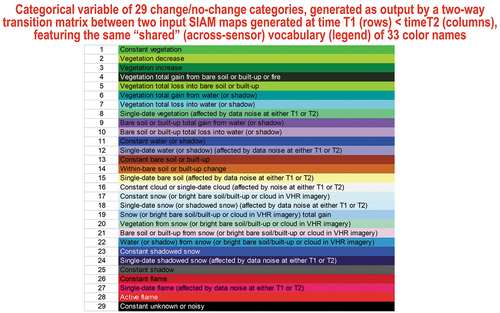
According to Section 2 to Section 4, an innovative semantics-enriched ARD product-pair and process gold standard is regarded as:

1. An inherently ill-posed cognitive information-as-data-interpretation task (refer to Subsection 3.3.3), where semantic relationship ‘ARD ⊂ EO-IU ⊂ CV ⊂ AGI ⊂ Cognitive science’ = Equation (3)(3) $\text{lsquo}\mathrm{A}\mathrm{R}\mathrm{D}\subset \mathrm{E}\mathrm{O}-\mathrm{I}\mathrm{U}\subset \mathrm{C}\mathrm{V}\subset \mathrm{A}\mathrm{G}\mathrm{I}\subset \mathrm{C}\mathrm{o}\mathrm{g}\mathrm{n}\mathrm{i}\mathrm{t}\mathrm{i}\mathrm{v}\mathrm{e}\mathrm{s}\mathrm{c}\mathrm{i}\mathrm{e}\mathrm{n}\mathrm{c}\mathrm{e}\text{rsquo}$(3) holds, see Figure 11. Hence, Bayesian inference constraints required for better conditioning an inherently ill-posed ARD-specific cognitive system solution are expected to be subset-of (a specialized version of, with inheritance) those proposed for an ‘EO-IU ⊂ CV ⊂ AGI’ system solution in Subsection 4.2.

2. Part-of (component-of, without inheritance) a “horizontal” (enabling) general-purpose application-independent and user-independent AGI4EO technology, see Figure 2. Coping with background conditions necessary to specialization in a new notion of Space Economy 4.0 (see Figure 10), AGI4EO pertains to the multi-disciplinary domain of cognitive science, where semantic relationship ‘Cognitive science ⊃ AGI ⊃ CV ⊃ EO-IU ⊃ ARD’ = Equation (3)(3) $\text{lsquo}\mathrm{A}\mathrm{R}\mathrm{D}\subset \mathrm{E}\mathrm{O}-\mathrm{I}\mathrm{U}\subset \mathrm{C}\mathrm{V}\subset \mathrm{A}\mathrm{G}\mathrm{I}\subset \mathrm{C}\mathrm{o}\mathrm{g}\mathrm{n}\mathrm{i}\mathrm{t}\mathrm{i}\mathrm{v}\mathrm{e}\mathrm{s}\mathrm{c}\mathrm{i}\mathrm{e}\mathrm{n}\mathrm{c}\mathrm{e}\text{rsquo}$(3) holds, see Figure 11. In more detail, an innovative AGI4EO technology can be accomplished at the space segment, referred to as AGI4Space encompassing so-called future intelligent EO satellites (EOportal, 2020; ESA – European Space Agency, 2019; Esposito et al., 2019a, 2019b; GISCafe News, 2018; Zhou, 2001), and/or midstream segment (NASA – National Aeronautics and Space Administration, 2019; CEOS – Committee on Earth Observation Satellites, 2018; DLR – Deutsches Zentrum für Luft-und Raumfahrt e.V. and VEGA Technologies, 2011; Dwyer et al., 2018; ESA – European Space Agency, 2015; Gómez-Chova et al., 2007; Helder et al., 2018; Houborga & McCabe, 2018; OHB, 2016; USGS – U.S. Geological Survey, 2018a, 2018b, 2018c; Vermote & Saleous, 2007), referred to as AGI4DIAS = Equation (1)(1) $\begin{array}{rl}& \text{lsquo}\mathrm{A}\mathrm{G}\mathrm{I}\text{-}\mathrm{e}\mathrm{n}\mathrm{a}\mathrm{b}\mathrm{l}\mathrm{e}\mathrm{d}\mathrm{D}\mathrm{I}\mathrm{A}\mathrm{S}=\mathrm{A}\mathrm{G}\mathrm{I}4\mathrm{D}\mathrm{I}\mathrm{A}\mathrm{S}=\mathrm{S}\mathrm{e}\mathrm{m}\mathrm{a}\mathrm{n}\mathrm{t}\mathrm{i}\mathrm{c}\mathrm{s}\text{-}\mathrm{e}\mathrm{n}\mathrm{a}\mathrm{b}\mathrm{l}\mathrm{e}\mathrm{d}\mathrm{D}\mathrm{I}\mathrm{A}\mathrm{S}2.0\\ & (\mathrm{D}\mathrm{I}\mathrm{A}\mathrm{S}{2}^{\mathrm{n}\mathrm{d}}\mathrm{g}\mathrm{e}\mathrm{n}\mathrm{e}\mathrm{r}\mathrm{a}\mathrm{t}\mathrm{i}\mathrm{o}\mathrm{n})=\mathrm{D}\mathrm{I}\mathrm{A}\mathrm{S}2.0=\mathrm{A}\mathrm{G}\mathrm{I}+\mathrm{D}\mathrm{I}\mathrm{A}\mathrm{S}1.0+\mathrm{S}\mathrm{C}\mathrm{B}\mathrm{I}\mathrm{R}+\mathrm{S}\mathrm{E}\mathrm{I}\mathrm{K}\mathrm{D}\text{rsquo}\end{array}$(1) , by both private and public EO big data providers.

3. Necessary-but-not-sufficient precondition of the RS meta-science community for developing a “horizontal” (enabling) AGI4DIAS infrastructure at the midstream segment (see Figure 10) = ‘AGI4DIAS = AGI-enabled DIAS = Semantics-enabled DIAS 2.0 = AGI + DIAS 1.0 + SCBIR + SEIKD’ = Equation (1)(1) $\begin{array}{rl}& \text{lsquo}\mathrm{A}\mathrm{G}\mathrm{I}\text{-}\mathrm{e}\mathrm{n}\mathrm{a}\mathrm{b}\mathrm{l}\mathrm{e}\mathrm{d}\mathrm{D}\mathrm{I}\mathrm{A}\mathrm{S}=\mathrm{A}\mathrm{G}\mathrm{I}4\mathrm{D}\mathrm{I}\mathrm{A}\mathrm{S}=\mathrm{S}\mathrm{e}\mathrm{m}\mathrm{a}\mathrm{n}\mathrm{t}\mathrm{i}\mathrm{c}\mathrm{s}\text{-}\mathrm{e}\mathrm{n}\mathrm{a}\mathrm{b}\mathrm{l}\mathrm{e}\mathrm{d}\mathrm{D}\mathrm{I}\mathrm{A}\mathrm{S}2.0\\ & (\mathrm{D}\mathrm{I}\mathrm{A}\mathrm{S}{2}^{\mathrm{n}\mathrm{d}}\mathrm{g}\mathrm{e}\mathrm{n}\mathrm{e}\mathrm{r}\mathrm{a}\mathrm{t}\mathrm{i}\mathrm{o}\mathrm{n})=\mathrm{D}\mathrm{I}\mathrm{A}\mathrm{S}2.0=\mathrm{A}\mathrm{G}\mathrm{I}+\mathrm{D}\mathrm{I}\mathrm{A}\mathrm{S}1.0+\mathrm{S}\mathrm{C}\mathrm{B}\mathrm{I}\mathrm{R}+\mathrm{S}\mathrm{E}\mathrm{I}\mathrm{K}\mathrm{D}\text{rsquo}\end{array}$(1) , suitable for augmenting the findable, accessible and reusable properties of the FAIR guiding principles for scientific data (product and process) management.

4. Necessary-but-not-sufficient precondition of the downstream segment for developing an ever-increasing ensemble of “vertical” (deep and narrow, specialized) domain- and user-specific VAPS in operational mode (Mazzucato & Robinson, 2017) (refer to Subsection 3.1), available for use by a potentially huge worldwide market of institutional and private end-users of space technology, encompassing the UN SDGs (UN – United Nations, Department of Economic and Social Affairs, 2021), in a new era of Space Economy 4.0, see Figure 10.

Intuitively, along the EO data and information processing chain required by a new notion of Space Economy 4.0 (see Figure 10), a specialization-through-competition second phase, consisting of “vertical” (deep and narrow) VAPS, whose specialization at the downstream segment is accomplished by analogy with “phenotypic” competition (Baraldi, 2017; Parisi, 1991; Piaget, 1970), is required to start as late as possible, i.e. vertical specialization does not start “from an absolute beginning” (Piaget, 1970), refer to Subsection 3.3.4. Rather, it starts in sequence to an enabling/initialization-through-cooperation first phase, consisting of a “horizontal” general-purpose user- and application-independent EO data-derived semantics-enriched ARD product-pair and process gold standard, accomplished in operational mode at the space segment and/or at the midstream segment, whose enabling capability is conceptually equivalent to a priori genotype (Baraldi, 2017; Parisi, 1991; Piaget, 1970). In more detail, semantics-enriched ARD product-pair and process suitability, encompassing interoperability (harmonization, opposite of heterogeneity), reusability, accuracy, efficiency, etc. (refer to Subsection 3.1), together with feasibility (doableness, practicality, viability), are jointly maximized (refer to Section 2) as pre-condition to augmented semantics-enriched data and information findability, accessibility and reusability in an AGI4DIAS = Equation (1)(1) $\begin{array}{rl}& \text{lsquo}\mathrm{A}\mathrm{G}\mathrm{I}\text{-}\mathrm{e}\mathrm{n}\mathrm{a}\mathrm{b}\mathrm{l}\mathrm{e}\mathrm{d}\mathrm{D}\mathrm{I}\mathrm{A}\mathrm{S}=\mathrm{A}\mathrm{G}\mathrm{I}4\mathrm{D}\mathrm{I}\mathrm{A}\mathrm{S}=\mathrm{S}\mathrm{e}\mathrm{m}\mathrm{a}\mathrm{n}\mathrm{t}\mathrm{i}\mathrm{c}\mathrm{s}\text{-}\mathrm{e}\mathrm{n}\mathrm{a}\mathrm{b}\mathrm{l}\mathrm{e}\mathrm{d}\mathrm{D}\mathrm{I}\mathrm{A}\mathrm{S}2.0\\ & (\mathrm{D}\mathrm{I}\mathrm{A}\mathrm{S}{2}^{\mathrm{n}\mathrm{d}}\mathrm{g}\mathrm{e}\mathrm{n}\mathrm{e}\mathrm{r}\mathrm{a}\mathrm{t}\mathrm{i}\mathrm{o}\mathrm{n})=\mathrm{D}\mathrm{I}\mathrm{A}\mathrm{S}2.0=\mathrm{A}\mathrm{G}\mathrm{I}+\mathrm{D}\mathrm{I}\mathrm{A}\mathrm{S}1.0+\mathrm{S}\mathrm{C}\mathrm{B}\mathrm{I}\mathrm{R}+\mathrm{S}\mathrm{E}\mathrm{I}\mathrm{K}\mathrm{D}\text{rsquo}\end{array}$(1) framework at the midstream segment, capable of SCBIR + SEIKD, see Figure 40.

Along the EO data and information processing chain required by a new notion of Space Economy 4.0 (see Figure 10), the conceptual and tangible boundary between a “horizontal” enabling first phase at the midstream segment and a “vertical” specialization (deep and narrow) second phase at the downstream segment is identified in our work by a new semantics-enriched ARD product-pair and process gold standard, to be accomplished at the space segment, in an AGI4Space framework, and/or midstream segment in an AGI4DIAS = Equation (1)(1) $\begin{array}{rl}& \text{lsquo}\mathrm{A}\mathrm{G}\mathrm{I}\text{-}\mathrm{e}\mathrm{n}\mathrm{a}\mathrm{b}\mathrm{l}\mathrm{e}\mathrm{d}\mathrm{D}\mathrm{I}\mathrm{A}\mathrm{S}=\mathrm{A}\mathrm{G}\mathrm{I}4\mathrm{D}\mathrm{I}\mathrm{A}\mathrm{S}=\mathrm{S}\mathrm{e}\mathrm{m}\mathrm{a}\mathrm{n}\mathrm{t}\mathrm{i}\mathrm{c}\mathrm{s}\text{-}\mathrm{e}\mathrm{n}\mathrm{a}\mathrm{b}\mathrm{l}\mathrm{e}\mathrm{d}\mathrm{D}\mathrm{I}\mathrm{A}\mathrm{S}2.0\\ & (\mathrm{D}\mathrm{I}\mathrm{A}\mathrm{S}{2}^{\mathrm{n}\mathrm{d}}\mathrm{g}\mathrm{e}\mathrm{n}\mathrm{e}\mathrm{r}\mathrm{a}\mathrm{t}\mathrm{i}\mathrm{o}\mathrm{n})=\mathrm{D}\mathrm{I}\mathrm{A}\mathrm{S}2.0=\mathrm{A}\mathrm{G}\mathrm{I}+\mathrm{D}\mathrm{I}\mathrm{A}\mathrm{S}1.0+\mathrm{S}\mathrm{C}\mathrm{B}\mathrm{I}\mathrm{R}+\mathrm{S}\mathrm{E}\mathrm{I}\mathrm{K}\mathrm{D}\text{rsquo}\end{array}$(1) framework, by both public and private EO big data providers.

6. Conclusions

Aiming at the convergence between Earth observation (EO) Big Data and Artificial General Intelligence (AGI), not to be confused with Artificial Narrow Intelligence (ANI), regarded herein as part-without-inheritance-of AGI in the multi-disciplinary domain of cognitive science, this methodological and survey paper consists of two parts, for the sake of readability. The present Part 1 is preliminary to the subsequent Part 2 (Baraldi et al., 2022).

In recent years, the notion of Earth observation (EO) optical sensory image-derived Analysis Ready Data (ARD), which includes quality layers to manage EO optical image uncertainty (vice versa, veracity), such as Cloud and Cloud-shadow masks, has been promoted by relevant portions of the remote sensing (RS) meta-science community to enable expert and non-expert end-users of space technology to access radiometrically calibrated EO large image databases ready for use in quantitative analytics of scientific quality, without requiring laborious EO image pre-processing for geometric and radiometric enhancement, preliminary to EO image processing (analysis).

The concept of ARD has been strictly coupled with the notion of EO big (raster-based) data cube, proposed by the RS community as innovative midstream EO technology.

Unfortunately, a community-agreed definition of EO big data cube does not exist yet, although several recommendations and implementations have been made. A community-agreed definition of ARD, to be adopted as standard baseline in EO data cube implementations, does not exist either. As a consequence, in common practice, many EO (raster-based) data cube definitions and implementations do not require ARD and, vice versa, an ever-increasing ensemble of new (supposedly better) ARD definitions and/or ARD-specific software implementations is proposed by the RS community, independently of a standardized/harmonized definition of EO big data cube.

To foster innovation across the global value chain required by a new notion of Space Economy 4.0, suitable for coping with grand societal challenges, such as the United Nations (UN) Sustainable Development Goals (SDGs) from year 2015 to 2030, this methodological and survey paper complies with the standard Findable Accessible Interoperable and Reusable (FAIR) guiding principles for scientific data (product and process) management to promote interoperability/ standardization/ harmonization, encompassing third-level semantic/ontological interoperability, among existing EO optical sensory image-derived Level 2/ ARD product definitions and software implementations, while overcoming their limitations investigated at the Marr five levels of understanding of an information processing system, specifically: (i) outcome and process requirements specification, (ii) information/knowledge representation, (iii) system design (architecture), (iv) algorithm and (v) implementation.

It is worth recalling here that, first, the standard FAIR criteria for scientific data (product and process) management overlap, in terms of reusability, synonym for regularity, with the popular engineering principles of structured system design, known as modularity, hierarchy and regularity, considered neither necessary nor sufficient, but highly recommended for system scalability. Moreover, property interoperability in the FAIR principles for scholarly/scientific digital data becomes, in the domain of analytical pipelines/processes, the tenet of system interoperability, encompassing a third semantic/ontological level of system interoperability.

Second, the Marr three more abstract levels of system understanding (refer to this Section above), specifically, outcome and process requirements specification, information/knowledge representation and system design, are typically considered the linchpin for success of an information processing system, rather than algorithm and implementation. This is in contrast with a large portion of the RS literature, where EO data processing and understanding systems are typically assessed and compared at the Marr two lowest (shallowest) levels of abstraction, specifically, algorithm and implementation.

Third, in a new notion of Space Economy 4.0, envisioned in 2017 by Mazzucato and Robinson in their original work for the European Space Agency (ESA), a first-stage “horizontal” (enabling) capacity building, coping with background conditions necessary to specialization, is preliminary to second-stage “vertical” (deep and narrow) specialization policies, suitable for coping with a potentially huge worldwide market of institutional and private end-users of space technology, encompassing grand societal challenges, such as the UN SDGs, see Figure 10.

Fourth, by definition, big data are characterized by the six Vs of volume, variety, veracity, velocity, volatility and value, to be coped with by big data management and processing systems. A special case of big data is large image database. An image is a 2D gridded data set, belonging to a (2D) image-plane. An obvious observation is that all images are data, but not all data are imagery. Hence, not all big data management and processing system solutions are expected to perform “well” when input with imagery, but computer vision (CV) systems, required to accomplish in operational mode the inherently ill-posed cognitive task of vision, synonym for 4D geospace-time scene-from-(2D) image reconstruction and understanding.

To overcome limitations of existing EO optical sensory image-derived Level 2/ARD product definitions and software implementations, an innovative semantics-enriched ARD product-pair and process gold standard is proposed to be community-agreed upon. Required to be systematically generated in operational mode at the space segment and/or midstream segment in a new notion of Space Economy 4.0, an innovative multi-sensor EO optical sensory image-derived semantics-enriched ARD co-product pair consists of:

1. An ARD numerical (subsymbolic and raster-based) co-product, consisting of an EO optical image, either panchromatic (PAN), multi-spectral (MS), super-spectral (SS) or hyper-spectral (HS), radiometrically calibrated into a sequence of top-of-atmosphere reflectance (TOARF) values, surface reflectance (SURF) values corrected from atmospheric, topographic and adjacency effects, and surface albedo values, corrected from bidirectional reflectance distribution function (BRDF) effects, in agreement with the intergovernmental Group on Earth Observations (GEO)-Committee on Earth Observation Satellites (CEOS) Quality Assurance Framework for Earth Observation (QA4EO) Calibration/Validation (Cal/Val) requirements.

   This ARD numerical co-product is systematically overlapped (stacked) with:

2. An ARD symbolic (categorical, semantic and vector-based) co-product, known as Scene Classification Map (SCM), whose thematic map legend (taxonomy, vocabulary) includes quality layers Cloud and Cloud-shadow, which improves and generalizes the existing well-known ESA EO Sentinel-2 imaging sensor-specific Level 2 SCM co-product.

In agreement with Bayesian inference, synonym for stratified/ masked/ class-conditional/ driven-by-prior-knowledge data analysis as viable alternative to unconditional/driven-without-prior-knowledge data analysis, an SCM is no optional by-product, but a mandatory information product required as input layer to make an inherently ill-posed radiometric correction problem of EO optical imagery better conditioned for numerical solution.

Noteworthy, both SCM (referred to as land cover) and surface albedo (referred to as albedo) are included in the list of terrestrial Essential Climate Variables (ECVs) defined by the World Climate Organization (WCO) (see Table 2), which complies with the GEO second implementation plan for years 2016–2025 of a new Global Earth Observation System of (component) Systems (GEOSS), regarded as expert EO data-derived information and knowledge system (see Figure 1), in agreement with the well-known Data-Information-Knowledge-Wisdom (DIKW) hierarchical conceptualization where, typically, information is defined in terms of data, knowledge in terms of information and wisdom in terms of knowledge, see Figure 12 and Figure 16.

Required to be systematically generated in operational mode at the space segment and/or midstream segment in a new notion of Space Economy 4.0, the proposed innovative semantics-enriched ARD co-product pair definition overcomes the shortcoming of existing ARD definitions and software implementations, which do not include “standardised and informative end user products required by national agencies tasked with coordinating implementation of [the UN] SDGs, [starting from] land cover and its change over time, that contribute to the mapping and reporting on 14 of the 17 SDGs”.

For the sake of readability, this paper consists of two parts. The present Part 1 is provided with a relevant survey value. First, it critically reviews notions of interest in the multi-disciplinary domain of cognitive science, considered as background knowledge of the RS meta-science, whose overarching goal is transformation of multi-source EO big sensory data, characterized by the six Vs of volume, variety, veracity, velocity, volatility and value, into operational, timely and comprehensive value-adding information products and services (VAPS), in compliance with (constrained by) the intergovernmental GEO-CEOS QA4EO Cal/Val requirements and with the well-known DIKW hierarchical conceptualization, see Figure 12 and Figure 16.

Second, the present Part 1 critically reviews and compares existing EO optical sensory image-derived Level 2/ARD product definitions and software implementations at the Marr five levels of understanding of an information processing system, where an original minimally dependent and maximally informative (mDMI) set of outcome and process (OP) quantitative quality indicators (Q²I) is adopted for inherently ill-posed multi-objective optimization, in agreement with the Pareto formal analysis of multi-objective optimization problems.

Regarded as background knowledge of the RS meta-science, keyword “information”, which is inherently vague, although widely adopted in a so-called era of Information and Communications Technology (ICT), is disambiguated into the two complementary not-alternative (co-existing) concepts of quantitative/unequivocal information-as-thing and qualitative/ equivocal/ inherently ill-posed information-as-data-interpretation. In addition, buzzword “Artificial Intelligence” is disambiguated into the two better-constrained notions of ANI as part-without-inheritance-of AGI.

In this context, the first original contribution of the present Part 1 is to formalize semantic relationships

Equation (6)(6) $x0026;\text{ANI=}[\text{DCNN}\subset \text{DL}\subset \text{ML}\text{logical0OR}\text{Traditional}\text{deductive}ArtificialIntelligencex0026;(\text{static}\text{expert}\text{systems},\text{non0adaptive}\text{to}\text{data},\text{also}\text{known}\text{as}\text{Good}\text{Old0Fashioned}x0026;ArtificialIntelligence,\text{GOFAI}]$(6) = ‘[Deep Convolutional Neural Network (DCNN) ⊂ Deep Learning (DL) ⊂ Machine learning-from-data (ML) logical-OR Traditional deductive Artificial Intelligence (static expert systems, non-adaptive to data, also known as Good Old-Fashioned Artificial Intelligence, GOFAI)] = ANI’, where ‘ANI → AGI ⊃ CV ⊃ EO image understanding (EO-IU) ⊃ ARD’ = Equation (5)(5) $\text{lsquo}\mathrm{A}\mathrm{R}\mathrm{D}\subset \mathrm{E}\mathrm{O}\text{-}\mathrm{I}\mathrm{U}\subset \mathrm{C}\mathrm{V}\subset \mathrm{A}\mathrm{G}\mathrm{I}\leftarrow \mathrm{A}\mathrm{N}\mathrm{I}\leftarrow \mathrm{M}\mathrm{L}\supset \mathrm{D}\mathrm{L}\supset \mathrm{D}\mathrm{e}\mathrm{e}\mathrm{p}\mathrm{C}\mathrm{o}\mathrm{n}\mathrm{v}\mathrm{o}\mathrm{l}\mathrm{u}\mathrm{t}\mathrm{i}\mathrm{o}\mathrm{n}\mathrm{a}\mathrm{l}\mathrm{N}\mathrm{e}\mathrm{u}\mathrm{r}\mathrm{a}\mathrm{l}\mathrm{N}\mathrm{e}\mathrm{t}\mathrm{w}\mathrm{o}\mathrm{r}\mathrm{k}\left(\mathrm{D}\mathrm{C}\mathrm{N}\mathrm{N}\right)\text{rsquo}$(5) ,

as working hypotheses (see Figure 11(a) and Figure 11(b)), where symbol ‘→’ denotes semantic relationship part-of (without inheritance) pointing from the supplier to the client, not to be confused with semantic relationship subset-of, meaning specialization with inheritance from the superset to the subset, whose symbol is ‘⊃’ (where superset is at left) in agreement with symbols adopted by the standard Unified Modeling Language (UML) for graphical modeling of object-oriented software. These postulates (axioms, first principles) contradict the increasingly popular belief that semantic relationship ‘A(G/N)I ⊃ ML ⊃ DL ⊃ DCNN’ = Equation (7)(7) $\text{lsquo}\mathrm{A}(\mathrm{G}/\mathrm{N})\mathrm{I}\supset \mathrm{M}\mathrm{L}\supset \mathrm{D}\mathrm{L}\supset \mathrm{D}\mathrm{C}\mathrm{N}\mathrm{N}\text{rsquo}$(7) holds, see Figure 11(c).

The second original contribution of the present Part 1 is to consider a novel semantics-enriched ARD product-pair and process gold standard, eligible for third-level semantic/ontological interoperability, as “horizontal” (enabling) general-purpose application- and user-independent AGI for EO (AGI4EO) technology. Coping with background conditions necessary to specialization in a new notion of Space Economy 4.0 (see Figure 10), a novel semantics-enriched ARD product-pair and process gold standard is required to be accomplished in operational mode at the space segment, in an AGI for space segment (AGI4Space) framework encompassing so-called future intelligent EO satellites, and/or midstream segment, in an AGI for Data and Information Access Services (AGI4DIAS) framework, by both private and public EO big data providers.

Availability of an innovative semantics-enriched ‘ARD ⊂ EO-IU ⊂ CV ⊂ AGI’ system in operational mode at the space segment and/or midstream segment, where ARD-specific product and process suitability (encompassing interoperability, reusability, etc.), together with feasibility (doableness, practicality), are jointly maximized, in compliance with the GEO-CEOS QA4EO Cal/Val requirements and the standard FAIR guiding principles for scientific data (product and process) management, to be included in a community-agreed mDMI set of OP-Q²Is, is regarded as:

1. Necessary-but-not-sufficient precondition of the RS community for developing a “horizontal” (enabling) AGI4DIAS infrastructure at the midstream = ‘AGI-enabled DIAS = Semantics-enabled DIAS 2.0 (DIAS 2^nd generation) = AGI + DIAS 1.0 + Semantic content-based image retrieval (SCBIR) + Semantics-enabled information/knowledge discovery (SEIKD)’ = Equation (1), suitable for augmenting the findable, accessible and reusable properties required by the FAIR guiding principles for scientific data (product and process) management.

   Synonym for AGI4DIAS = Equation (1)(1) $\begin{array}{rl}& \text{lsquo}\mathrm{A}\mathrm{G}\mathrm{I}\text{-}\mathrm{e}\mathrm{n}\mathrm{a}\mathrm{b}\mathrm{l}\mathrm{e}\mathrm{d}\mathrm{D}\mathrm{I}\mathrm{A}\mathrm{S}=\mathrm{A}\mathrm{G}\mathrm{I}4\mathrm{D}\mathrm{I}\mathrm{A}\mathrm{S}=\mathrm{S}\mathrm{e}\mathrm{m}\mathrm{a}\mathrm{n}\mathrm{t}\mathrm{i}\mathrm{c}\mathrm{s}\text{-}\mathrm{e}\mathrm{n}\mathrm{a}\mathrm{b}\mathrm{l}\mathrm{e}\mathrm{d}\mathrm{D}\mathrm{I}\mathrm{A}\mathrm{S}2.0\\ & (\mathrm{D}\mathrm{I}\mathrm{A}\mathrm{S}{2}^{\mathrm{n}\mathrm{d}}\mathrm{g}\mathrm{e}\mathrm{n}\mathrm{e}\mathrm{r}\mathrm{a}\mathrm{t}\mathrm{i}\mathrm{o}\mathrm{n})=\mathrm{D}\mathrm{I}\mathrm{A}\mathrm{S}2.0=\mathrm{A}\mathrm{G}\mathrm{I}+\mathrm{D}\mathrm{I}\mathrm{A}\mathrm{S}1.0+\mathrm{S}\mathrm{C}\mathrm{B}\mathrm{I}\mathrm{R}+\mathrm{S}\mathrm{E}\mathrm{I}\mathrm{K}\mathrm{D}\text{rsquo}\end{array}$(1) is semantics-enabled EO big raster-based numerical data and vector-based categorical (symbolic, semi-symbolic or subsymbolic, see Figure 15) information cube management system, see Figure 39. It is proposed as viable alternative to existing EO big (raster-based) data cube management systems, including the European Commision (EC) DIAS 1.0 realizations, where the CEOS ARD for Land Optical Surface Reflectance (CARD4L-OSR) product definition (see Figure 35) is typically adopted as standard ARD baseline, if any, and to prototypical content-based image retrieval (CBIR) systems, see Figure 4. Due to lack of meaning/semantics in their adopted ARD baseline, if any, existing EO data cubes are typically affected by the data-rich information-poor (DRIP) syndrome.

   Noteworthy, the notion of AGI4DIAS = Equation (1)(1) $\begin{array}{rl}& \text{lsquo}\mathrm{A}\mathrm{G}\mathrm{I}\text{-}\mathrm{e}\mathrm{n}\mathrm{a}\mathrm{b}\mathrm{l}\mathrm{e}\mathrm{d}\mathrm{D}\mathrm{I}\mathrm{A}\mathrm{S}=\mathrm{A}\mathrm{G}\mathrm{I}4\mathrm{D}\mathrm{I}\mathrm{A}\mathrm{S}=\mathrm{S}\mathrm{e}\mathrm{m}\mathrm{a}\mathrm{n}\mathrm{t}\mathrm{i}\mathrm{c}\mathrm{s}\text{-}\mathrm{e}\mathrm{n}\mathrm{a}\mathrm{b}\mathrm{l}\mathrm{e}\mathrm{d}\mathrm{D}\mathrm{I}\mathrm{A}\mathrm{S}2.0\\ & (\mathrm{D}\mathrm{I}\mathrm{A}\mathrm{S}{2}^{\mathrm{n}\mathrm{d}}\mathrm{g}\mathrm{e}\mathrm{n}\mathrm{e}\mathrm{r}\mathrm{a}\mathrm{t}\mathrm{i}\mathrm{o}\mathrm{n})=\mathrm{D}\mathrm{I}\mathrm{A}\mathrm{S}2.0=\mathrm{A}\mathrm{G}\mathrm{I}+\mathrm{D}\mathrm{I}\mathrm{A}\mathrm{S}1.0+\mathrm{S}\mathrm{C}\mathrm{B}\mathrm{I}\mathrm{R}+\mathrm{S}\mathrm{E}\mathrm{I}\mathrm{K}\mathrm{D}\text{rsquo}\end{array}$(1) fully complies with the GEO second mandate of a GEOSS for years 2016–2025 (see Figure 1), expected to evolve from an EO big data sharing infrastructure, intuitively referred to as data-centric approach, to an expert EO data-derived information and knowledge system, intuitively referred to as knowledge-driven approach, capable of supporting decision-making by delivering to end-users high-level Essential (Community) Variables, rather than low-level EO big sensory data, to successfully cope with challenges along all six community-agreed degrees (dimensionalities, axes) of complexity of big data, known as the six Vs of volume, variety, veracity, velocity, volatility and value.

   For example, by focusing on the delivery to end-users of EO sensory data-derived Essential (Community) Variables as information sets relevant for decision-making, in place of delivering low-level EO big sensory data, the Big Data requirements of the GEOSS digital Common Infrastructure are expected to decrease (see Figure 1), in compliance with the well-known DIKW hierarchical conceptualization, see Figure 12 and Figure 16.

2. Necessary-but-not-sufficient precondition of the downstream segment for developing an ever-increasing ensemble of “vertical” (deep and narrow, specialized) domain- and user-specific VAPS in operational mode, available for use by a potentially huge worldwide market of institutional and private end-users of space technology, encompassing the UN SDGs at global scale, in a new notion of Space Economy 4.0, see Figure 10.

In summary, the present Part 1 identifies an innovative semantics-enriched EO optical image-derived ARD product-pair and process gold standard as linchpin for success of a new Space Economy 4.0. Equivalent to a necessary-but-not-sufficient precondition for a new notion of Space Economy 4.0 to become realistic/ feasible/ doable, an innovative semantics-enriched ARD product-pair and process gold standard is:

• Required to be accomplished in operational mode at the space segment, in an AGI4Space framework encompassing so-called future intelligent EO satellites, and/or midstream segment, in an AGI4DIAS = Equation (1)(1) $\begin{array}{rl}& \text{lsquo}\mathrm{A}\mathrm{G}\mathrm{I}\text{-}\mathrm{e}\mathrm{n}\mathrm{a}\mathrm{b}\mathrm{l}\mathrm{e}\mathrm{d}\mathrm{D}\mathrm{I}\mathrm{A}\mathrm{S}=\mathrm{A}\mathrm{G}\mathrm{I}4\mathrm{D}\mathrm{I}\mathrm{A}\mathrm{S}=\mathrm{S}\mathrm{e}\mathrm{m}\mathrm{a}\mathrm{n}\mathrm{t}\mathrm{i}\mathrm{c}\mathrm{s}\text{-}\mathrm{e}\mathrm{n}\mathrm{a}\mathrm{b}\mathrm{l}\mathrm{e}\mathrm{d}\mathrm{D}\mathrm{I}\mathrm{A}\mathrm{S}2.0\\ & (\mathrm{D}\mathrm{I}\mathrm{A}\mathrm{S}{2}^{\mathrm{n}\mathrm{d}}\mathrm{g}\mathrm{e}\mathrm{n}\mathrm{e}\mathrm{r}\mathrm{a}\mathrm{t}\mathrm{i}\mathrm{o}\mathrm{n})=\mathrm{D}\mathrm{I}\mathrm{A}\mathrm{S}2.0=\mathrm{A}\mathrm{G}\mathrm{I}+\mathrm{D}\mathrm{I}\mathrm{A}\mathrm{S}1.0+\mathrm{S}\mathrm{C}\mathrm{B}\mathrm{I}\mathrm{R}+\mathrm{S}\mathrm{E}\mathrm{I}\mathrm{K}\mathrm{D}\text{rsquo}\end{array}$(1) framework, by both public and private EO big data providers, and it is

• Considered as a conceptual and tangible boundary between a “horizontal” enabling first phase at the midstream segment and a “vertical” specialization (deep and narrow) second phase at the downstream segment in a new notion of Space Economy 4.0, see Figure 10.

Based on takeaways about an innovative ARD product-pair and process gold standard proposed in Subsection 5.2 of the present Part 1, the subsequent Part 2 of this two-part paper provides, first, at the Marr first level of system understanding, a novel EO optical image-derived ARD product-pair requirements specification.

Second, ARD software system (process) solutions are investigated at the Marr five levels of processing system understanding. As proof of feasibility in addition to proven suitability, existing ARD software subsystem solutions, ranging from software subsystem design to algorithm and implementation, are selected from the scientific literature to benefit from their technology readiness level (TRL).

Acknowledgments

Andrea Baraldi thanks Prof. Raphael Capurro for his hospitality, patience, politeness and open-mindedness. The authors wish to thank the editors and reviewers for their competence, patience and willingness to help.

Disclosure statement

No potential conflict of interest was reported by the authors.

Data availability statement

Data sharing is not applicable to this article as no new data were created or analyzed in this study.

Supplemental data

Supplemental data for this article can be accessed here.

Correction Statement

This article has been corrected with minor changes. These changes do not impact the academic content of the article.

Additional information

Funding

This work was supported in part by the Austrian Research Promotion Agency (FFG), under the: (i) ASAP 16 project call, project title: SemantiX - A cross-sensor semantic EO data cube to open and leverage essential climate variables with scientists and the public, Grant ID: 878939, and (ii) ASAP 17 project call, project title: SIMS - Soil sealing identification and monitoring system, Grant ID: 885365.

Notes on contributors

Andrea Baraldi

Andrea Baraldi received his Laurea (M.S.) degree in Electronic Engineering from the University of Bologna, Italy, in 1989, a Master Degree in Software Engineering from the University of Padua, Italy, in 1994, and a PhD degree in Agricultural and Food Sciences from the University of Naples Federico II, Italy, in 2017. He has held research positions at the Italian Space Agency (ASI), Rome, Italy (2018-2021), Dept. of Geoinformatics (Z-GIS), Univ. of Salzburg, Austria (2014-2017), Dept. of Geographical Sciences, University of Maryland (UMD), College Park, MD (2010-2013), European Commission Joint Research Centre (EC-JRC), Ispra, Italy (2000-2002; 2005-2009), International Computer Science Institute (ICSI), Berkeley, CA (1997-1999), European Space Agency Research Institute (ESRIN), Frascati, Italy (1991-1993), Italian National Research Council (CNR), Bologna, Italy (1989, 1994-1996, 2003-2004). In 2009, he founded Baraldi Consultancy in Remote Sensing, a one-man company located in Modena, Italy. In Feb. 2014, he was appointed with a Senior Scientist Fellowship at the German Aerospace Center (DLR), Oberpfaffenhofen, Germany. In Feb. 2015, he was a visiting scientist at the Ben Gurion Univ. of the Negev, Sde Boker, Israel, funded by the European Commission FP7 Experimentation in Ecosystem Research (ExpeER) project. His main research interests center on image pre-processing and understanding, with special emphasis on the research and development of automatic near real-time Earth observation spaceborne/airborne image understanding systems in operational mode, consistent with human visual perception. Dr. Baraldi’s awards include the Copernicus Masters Prize Austria 2020, Copernicus Masters - Winner 2015 of the T-Systems Big Data Challenge and the 2nd-place award at the 2015 IEEE GRSS Data Fusion Contest. He served as Associate Editor of the IEEE Trans. Neural Networks journal from 2001 to 2006.

Luca D. Sapia

Luca D. Sapia received his Master’s Degree in Civil Engineering from the University of Bologna, Italy, in 2015. He has held research positions at Arpae Emilia-Romagna, Bologna, Italy (2015-2020), Department of Civil, Chemical, Environmental, and Materials Engineering (DICAM), University of Bologna, Bologna, Italy (2018-2019), Interdepartmental Center for Energy and the Environment (CIDEA), University of Parma, Parma, Italy (2016-2018). From 2019 to 2021, he worked for the European Space Agency (ESA) at Serco Italy as science support specialist and Earth Observation (EO) products analysis expert for the Copernicus data Quality Control (CQC) service. Currently, he is Program Manager of the Earth Observation Applications Unit at CGI Italy. His main interests center on EO data acquisition and systematic generation of EO data-derived value-adding information products and services. In the last years, he focused on developing, validating and transferring EO technologies to the Italian agricultural market. He is the inventor of the “LET” (Landsat EvapoTranspiration) operational service for the detection of unauthorized water withdrawals for irrigation use in agriculture.

Dirk Tiede

Dirk Tiede, PhD, is Associate Professor at the University of Salzburg, Department of Geoinformatics – Z_GIS, Austria, and head of the research area EO Analytics. His research focuses on methodological developments in image analysis using optical EO data, object-based methodologies and process automation in the context of Big EO data analysis. Research fields include environmental monitoring and support of humanitarian relief operations, for which he received the Christian-Doppler-Award of the Federal State of Salzburg in 2014, the Copernicus Master Award “Big Data Challenge” in 2015, the Copernicus Prize Austria in 2020 and was ranked 2nd in the IEEE GRSS Data Fusion Contest 2015.

Martin Sudmanns

Martin Sudmanns, PhD, is postdoctoral researcher at the University of Salzburg, Department of Geoinformatics – Z_GIS, Austria with a research focus on Geoinformatics, computer-based representation of natural phenomena in spatial data models, spatio-temporal Earth observation analysis in the context of data cubes and big EO data. He received the Copernicus Master Award “Big Data Challenge” in 2015 and the Copernicus Prize Austria in 2020.

Hannah L. Augustin

Hannah L. Augustin, MSc, is a PhD researcher in Earth observation (EO) Analytics at the University of Salzburg, Department of Geoinformatics – Z_GIS, Austria with a research focus on semantic EO data cubes, automated and transferable processes for generating EO-informed indicators from big optical EO imagery and related geovisualisation. She was part of the team awarded with the Copernicus Prize Austria in 2020.

Stefan Lang

Stefan Lang, PhD, Geographer, GIS and Remote Sensing specialist and Associate Professor at the University of Salzburg, Research Coordinator at Z_GIS and co-head of the Earth Observation division. He is leading the Christian-Doppler Laboratory for geo-humanitarian action, with a research focus on OBIA, hybrid AI, systems thinking, data assimilation, multi-scale regionalisation, validation.

References

- Adamo, M., Tomaselli, V., Tarantino, C., Vicario, S., Veronico, G., Lucas, R., & Blonda, P. (2020). Knowledge-based classification of grassland ecosystem based on multi-temporal WorldView-2 data and FAO-LCCS taxonomy. Remote Sensing, 12(1447), 1–31. doi:10.3390/rs12091447
- Adams, J. B., Donald, E. S., Kapos, V., Almeida Filho, R., Roberts, D. A., Smith, M. O., & Gillespie, A. R. (1995). Classification of multispectral images based on fractions of endmembers: Application to land-cover change in the Brazilian Amazon. Remote Sensing of Environment, 52, 137–154. doi:10.1016/0034-4257(94)00098-8
- Ahlqvist, O. (2008). In search of classification that supports the dynamics of science: the FAO Land Cover Classification System and proposed modifications. Environment and planning. B, Planning & design, 35, 169–186. doi:10.1068/b3344
- Airbus. (2018, October 11). OneAtlas Basemap Flyer. Retrieved from https://www.intelligence-airbusds.com/files/pmedia/public/r50152_9_oneatlas_basemap_flyer.pdf
- APS - Association for Psychological Science. (2008). New study explains why the future is more important than the past. Retrieved from https://www.psychologicalscience.org/news/releases/new-study-explains-why-the-future-is-more-important-than-the-past.html
- Arocena, J., Lozano, J., Quartulli, M., Olaizola, I., & Bermudez, J. (2015, July 18–25). Linked open data for raster and vector geospatial information processing. In Proc. of the 2015 IEEE Int. Geoscience and Remote Sensing Symposium (IGARSS), Milan, Italy, (pp. 5023–5026).
- ASI - Agenzia Spaziale Italiana. (2020, December 3). PRISMA Products Specification Document. Issue 2.3, Retrieved from http://prisma.asi.it/missionselect/docs/PRISMA%20Product%20Specifications_Is2_3.pdf
- Augustin, H., Sudmanns, M., Tiede, D., & Baraldi, A. (2018, July 3–6). A semantic Earth observation data cube for monitoring environmental changes during the Syrian conflict. In Proceedings of the AGIT 2018, Salzburg, Austria, (pp. 214–227). doi: 10.1553/giscience2018_01_s214
- Augustin, H., Sudmanns, M., Tiede, D., Lang, S., & Baraldi, A. (2019). Semantic earth observation data cubes. 102 Data, 4, 1–19. doi:10.3390/data4030102.
- Baatz, M., & Schäpe, A. (2000). Multiresolution segmentation: An optimization approach for high quality multi-scale image segmentation. In J. Strobl (Ed.), Angewandte geographische informationsverarbeitung XII, Vol 58, 12–23. Berlin, Germany: Herbert Wichmann Verlag.
- Ball, J. (2021, March 2). Using meaning as universal knowledge representation. Medium. Accessed 9 March 2021. Retrieved from https://medium.com/pat-inc/using-meaning-as-universal-knowledge-representation-f4b2b72ea4e0
- Ball, P. (2013, March5). Moore’s law is not just for computers. Nature News, doi:10.1038/nature.2013.12548
- Baraldi, A. (2009). Impact of radiometric calibration and specifications of spaceborne optical imaging sensors on the development of operational automatic remote sensing image understanding systems. IEEE Journal of Selected Topics in Applied Earth Observations and Remote Sensing, 2(5), 104–134. doi:10.1109/JSTARS.2009.2023801
- Baraldi, A. (2017, May 16). Pre-processing, classification and semantic querying of large-scale Earth observation spaceborne/airborne/terrestrial image databases: Process and product innovations. Ph.D. dissertation in Agricultural and Food Sciences, University of Naples “Federico II”, Department of Agricultural Sciences, Italy. Ph.D. defense, Retrieved from http://www.fedoa.unina.it/11724/1/TesiDottorato_Unina_XXIX_AB_EO-IU4SQ_v4_RGB_10April2017.pdf
- Baraldi, A. (2019a). Satellite Image Automatic Mapper™ (SIAM™) as a Service (SIAMaaS) Demonstrator installed onto the Serco’s ONDA Data and Information Access Services (DIAS) Marketplace. Accessed 9 Jan 2020. Retrieved from https://indoors2001.zgis.at/portal/apps/MapJournal/index.html?appid=1ab1e4a63ce24da2b69e5cfa3e4f1907
- Baraldi, A. (2019b, May 13-19). Radiometric Calibration/Validation of Earth observation small satellite constellations: The PlanetScope case of 130+ Dove 3U CubeSat 5kg nano-satellites.In (poster session) ESA Living Planet Symposium, Milan, Italy. Retrieved from https://www.researchgate.net/publication/333209805_Radiometric_CalibrationValidation_of_Earth_observation_small_satellite_constellations_The_PlanetScope_case_of_130_Dove_3U_CubeSat_5kg_nano-satellites/link/5cf60ec292851c4dd026f38c/download
- Baraldi, A., & Alpaydin, E. (2002a). Constructive feedforward ART clustering networks - Part I. IEEE Transactions on Neural Networks, 13(3), 645–661. doi:10.1109/TNN.2002.1000130
- Baraldi, A., & Alpaydin, E. (2002b). Constructive feedforward ART clustering networks - Part II. IEEE Transactions on Neural Networks, 13(3), 662–677. doi:10.1109/TNN.2002.1000131
- Baraldi, A., & Boschetti, L. (2012a). Operational automatic remote sensing image understanding systems: Beyond Geographic Object-Based and Object-Oriented Image Analysis (GEOBIA/GEOOIA) - Part 1: Introduction. Remote Sensing, 4(9), 2694–2735. doi:10.3390/rs4092694
- Baraldi, A., & Boschetti, L. (2012b). Operational automatic remote sensing image understanding systems: Beyond Geographic Object-Based and Object-Oriented Image Analysis (GEOBIA/GEOOIA) - Part 2: Novel system architecture, information/ knowledge representation, algorithm design and implementation. Remote Sensing, 4(9), 2768–2817. doi:10.3390/rs4092768
- Baraldi, A., Boschetti, L., & Humber, M. (2014). Probability sampling protocol for thematic and spatial quality assessments of classification maps generated from spaceborne/airborne very high resolution images. IEEE Transactions on Geoscience and Remote Sensing, 52(1). Part: 2, 701–760. doi:10.1109/TGRS.2013.2243739.
- Baraldi, A., Bruzzone, L., & Blonda, P. (2006). A multi-scale expectation-maximization semisupervised classifier suitable for badly-posed image classification. IEEE Transactions on Image Processing, 15(8), 2208–2225. doi:10.1109/TIP.2006.875220
- Baraldi, A., Bruzzone, L., Blonda, P., & Carlin, L. (2006). Badly-posed classification of remotely sensed images - An experimental comparison of existing data labeling systems. IEEE Transactions on Geoscience and Remote Sensing, 44(1), 214–235. doi:10.1109/TGRS.2005.859362
- Baraldi, A., Durieux, L., Simonetti, D., Conchedda, G., Holecz, F., & Blonda, P. (2010a). Automatic spectral rule-based preliminary classification of radiometrically calibrated SPOT-4/-5/IRS, AVHRR/MSG, AATSR, IKONOS/QuickBird/OrbView/GeoEye and DMC/SPOT-1/-2 imagery – Part I: System design and implementation. IEEE Transactions on Geoscience and Remote Sensing, 48(3), 1299–1325. doi:10.1109/TGRS.2009.2032457
- Baraldi, A., Durieux, L., Simonetti, D., Conchedda, G., Holecz, F., & Blonda, P. (2010b). Automatic Automatic spectral rule-based preliminary classification of radiometrically calibrated SPOT-4/-5/IRS, AVHRR/MSG, AATSR, IKONOS/QuickBird/OrbView/GeoEye and DMC/SPOT-1/-2 imagery – Part II: Classification accuracy assessment. IEEE Transactions on Geoscience and Remote Sensing, 48(3), 1326–1354. doi:10.1109/TGRS.2009.2032064
- Baraldi, A., Gironda, M., & Simonetti, D. (2010). Operational two-stage stratified topographic correction of spaceborne multi-spectral imagery employing an automatic spectral rule-based decision-tree preliminary classifier. IEEE Transactions on Geoscience and Remote Sensing, 48, 112–146. doi:10.1109/TGRS.2009.2028017
- Baraldi, A., Humber, M. L., Tiede, D., & Lang, S. (2018a). GEO-CEOS stage 4 validation of the Satellite Image Automatic Mapper lightweight computer program for ESA Earth observation Level 2 product generation – Part 1: Theory. Cogent Geoscience, 4, doi: 10.1080/23312041.2018.1467357
- Baraldi, A., Humber, M. L., Tiede, D., & Lang, S. (2018b). GEO-CEOS stage 4 validation of the Satellite Image Automatic Mapper lightweight computer program for ESA Earth observation Level 2 product generation – Part 2: Validation. Cogent Geoscience, 4, doi: 10.1080/23312041.2018.1467254
- Baraldi, A., Lang, S., Tiede, D., & Blaschke, T. (2018, June 18-22). Earth observation big data analytics in operational mode for GIScience applications – The (GE)OBIA acronym(s) reconsidered. In Proceedings of the GEOBIA 2018, Montpellier, France.
- Baraldi, A., Puzzolo, V., Blonda, P., Bruzzone, L., & Tarantino, C. (2006). Automatic spectral rule-based preliminary mapping of calibrated Landsat TM and ETM+ images. IEEE Transactions on Geoscience and Remote Sensing, 44, 2563–2586. doi:10.1109/TGRS.2006.874140
- Baraldi, A., Sapia, L. D., Tiede, D., Sudmann, M., Augustin, H. L., & Lang, S. (2022). Innovative Analysis Ready Data (ARD) product and process requirements, software system design, algorithms and implementation at the midstream as necessary-but-not-sufficient precondition of the downstream in a new notion of Space Economy 4.0 - Part 2: Software developments. Big Earth Data. doi: 10.1080/20964471.2021.2017582
- Baraldi, A., & Soares, J. V. B. (2017). Multi-Objective software suite of two-dimensional shape descriptors for object-based image analysis, subjects: Computer vision and pattern recognition (cs.CV). arXiv: 1701.01941. Accessed 8 Jan. 2020. Retrieved from https://arxiv.org/ftp/arxiv/papers/1701/1701.01941.pdf
- Baraldi, A., & Tiede, D. (2018a). AutoCloud+, a “universal” physical and statistical model-based 2D spatial topology-preserving software for cloud/cloud–shadow detection in multi-sensor single-date Earth observation multi-spectral imagery – Part 1: Systematic ESA EO Level 2 product generation at the ground segment as broad context. ISPRS International Journal of Geo-Information, 7, 457. Accessed 8 January 2020. Retrieved from http://www.mdpi.com/2220-9964/7/12/457/pdf. doi:10.3390/ijgi7120457
- Baraldi, A., & Tiede, D. (2018b). AutoCloud+, a “universal” physical and statistical model-based 2D spatial topology-preserving software for cloud/cloud–shadow detection in multi-sensor single-date Earth observation multi-spectral imagery – Part 2: Outcome and process requirements specification, information/ knowledge representation, system design, algorithm, implementation and preliminary experimental results. ISPRS International Journal of Geo-Information, 7, 457. Accessed 8 January 2020. Retrieved from https://www.mdpi.com/2220-9964/7/12/457#supplementary
- Baraldi, A., Tiede, D., Sudmanns, M., Belgiu, M., & Lang, S. (2016, September 14–16). Automated near real-time Earth observation level 2 product generation for semantic querying. In Proceedings of the GEOBIA 2016, University of Twente, Faculty of Geo-Information and Earth Observation (ITC), Enschede, The Netherlands.
- Baraldi, A., Tiede, D., Sudmanns, M., & Lang, S. (2017, March 28–30). Systematic ESA EO Level 2 product generation as precondition to semantic content-based image retrieval and information/ knowledge discovery in EO image databases. In Proceedings of the BiDS’17 Conference on Big Data from Space, Toulouse, France.
- Barrett, L. F. (2017). How emotions are made: The secret life of the brain. New York: Houghton Mifflin Harcourt.
- Bartoš, M. (2017). Cloud and shadow detection in satellite imagery. Master’s Thesis, Computer Vision and Image Processing, Faculty of Electrical Engineering, Department of Cybernetics, Czech Technical University, Prague, Czech Republic.
- Baumann, O. (2017). The Datacube Manifesto. Retrieved from https://external.ogc.org/twiki_public/pub/CoveragesDWG/Datacubes/The-Datacube-Manifesto.pdf
- Belgiu, M., Drǎguţ, L., & Strobl, J. (2014). Quantitative evaluation of variations in rule-based classifications of land cover in urban neighbourhoods using WorldView-2 imagery. ISPRS Journal of Photogrammetry and Remote Sensing, 87, 205–215. doi:10.1016/j.isprsjprs.2013.11.007
- Belward, A. S., & Skøien, J. O. (2015). Who launched what, when and why; trends in global land-cover observation capacity from civilian earth observation satellites. ISPRS Journal of Photogrammetry and Remote Sensing, 103, 115–128. doi:10.1016/j.isprsjprs.2014.03.009
- Benavente, R., Vanrell, M., & Baldrich, R. (2008). Parametric fuzzy sets for automatic color naming. Journal of the Optical Society of America A, 25(10), 2582–2593. doi:10.1364/JOSAA.25.002582
- Beniaguev, D., Segev, I., & London, M. (2021). Single cortical neurons as deep artificial neural networks. Neuron, 109(17), 2727–2739. doi:10.1016/j.neuron.2021.07.002
- Berlin, B., & Kay, P. (1969). Basic Color terms: Their universality and evolution. Berkeley, CA, USA: University of California.
- Bernus, P., & Noran, O. (2017). Data Rich–But Information Poor. In L. Camarinha-Matos, H. Afsarmanesh, & R. Fornasiero (Eds.). PRO-VE 2017, IFIP advances in information and communication technology, Collaboration in a Data-Rich World, Vol. 506, 206–214. Berlin, Germany: Springer.
- Bharath, A., & Petrou, M. (2008). Next Generation Artificial Vision Systems – Reverse Engineering the Human Visual System. Boston, MA, USA: Artech House.
- Bilal, M., Nazeer, M., Nichol, J. E., Bleiweiss, M. P., Qiu, Z., Jäkel, E., … Lolli, S. (2019). A Simplified and Robust Surface Reflectance Estimation Method (SREM) for use over diverse land surfaces using multi-sensor data. Remote Sensing, 11(1344), 1–24. doi:10.3390/rs11111344
- Bills, N. J. (2020, September 17). Can we kill the term “Artificial Intelligence” yet? Better Programming, Retrieved from https://betterprogramming.pub/kill-artificial-intelligence-7bc02f85ea70
- Bishop, C. M. (1995). Neural networks for pattern recognition. Oxford, United Kingdom: Clarendon.
- Bishop, M. P., & Colby, J. D. (2002). Anisotropic reflectance correction of SPOT-3 HRV imagery. International Journal of Remote Sensing, 23, 2125–2131. doi:10.1080/01431160110097231
- Bishop, M. P., Shroder, J. F., & Colby, J. D. (2003). Remote sensing and geomorphometry for studying relief production in high mountains. Geomorphology, 55, 345–361. doi:10.1016/S0169-555X(03)00149-1
- Bittner, T., Donnelly, M., & Winter, S. (2005). Ontology and semantic interoperability. Large-Scale 3D Data Integration, CRC Press, 139–161. doi:10.1201/9781420036282.pt3
- Blaschke, T., Hay, G. J., Kelly, M., Lang, S., Hofmann, P., Addink, E., … Tiede, D. (2014). Geographic object-based image analysis - towards a new paradigm. ISPRS Journal of Photogrammetry and Remote Sensing, 87, 180–191. doi:10.1016/j.isprsjprs.2013.09.014
- Bojinski, S., Verstraete, M., Peterson, T. C., Richter, C., Simmons, A., & Zemp, M. (2014). The concept of Essential Climate Variables in support of climate research, applications and policy. American Meteorological Society, 9, 1431–1443. doi:10.1175/BAMS-D-13-00047.1
- Borduas, N., & Donahue, N. M. (2018). Chapter 3.1 - The Natural Atmosphere. In B. Török & T. Dransfield (Eds.), Green Chemistry, (pp. 131–150). Oxford, UK: Elsevier. doi: 10.1016/C2015-0-05674-X.
- Boschetti, L., Flasse, S. P., & Brivio, P. A. (2004). Analysis of the conflict between omission and commission in low spatial resolution dichotomic thematic products: The Pareto boundary. Remote Sensing of Environment, 91, 280–292. doi:10.1016/j.rse.2004.02.015
- Bossard, M., Feranec, J., & Otahel, J. (2000). CORINE Land Cover Technical Guide–Addendum 2000. Technical report No 40, Copenhagen, Denmark: European Environment Agency.
- Bourdakos, N. (2017). Capsule Networks Are Shaking up AI — Here’s How to Use Them, 2017. Accessed 8 Jan. 2020. Retrieved from https://hackernoon.com/capsule-networks-are-shaking-up-ai-heres-how-to-use-them-c233a0971952
- Bowers, J. S., & Davis, C. J. (2012). Bayesian just-so stories in psychology and neuroscience. Psychological Bulletin, 138(6), 389. doi:10.1037/a0026450
- Boynton, R. M. (1990). Human color perception. In Science of Vision, K. N. Leibovic (Ed.), New York, NY, USA: Springer (pp. 211–253).
- Brendel, W. (2019, February 6). Neural Networks seem to follow a puzzlingly simple strategy to classify images. Medium, Retrieved from https://medium.com/bethgelab/neural-networks-seem-to-follow-a-puzzlingly-simple-strategy-to-classify-images-f4229317261f
- Brendel, W. and Bethge, M. (2019). Approximating CNNs with bag-of-local-features models works surprisingly well on ImageNet. In International Conference on Learning Representations (ICRL) 2019, New Orleans (LA), USA, 6–9 May 2019. Accessed 7 Jan. 2020. Retrieved from https://openreview.net/pdf?id=SkfMWhAqYQ
- Brinkworth, J. (1992). Software Quality Management - A Pro-active approach. New York, NY, USA: Prentice.
- Britannica Online Encyclopedia. (2017). Von Neumann machine. Retrieved from https://www.britannica.com/technology/von-Neumann-machine
- Buonomano, D. (2018). Your Brain is a Time Machine: The Neuroscience and Physics of Time. New York, NY, USA: W. W. Norton & Company.
- Burt, P., & Adelson, E. (1983). The Laplacian pyramid as a compact image code. IEEE Transactions on Communications, 31(4), 532–540. doi:10.1109/TCOM.1983.1095851
- Buyong, T. (2007). Spatial data analysis for geographic information science. Kuala Lumpur, Malaysia: Penerbit.
- Camara, G. (2017, November 28-30). e-Sensing: Big Earth observation data analytics for land use and land cover change information. In ESA Big Data from Space (BiDS) 2017 Conference Proceedings, Toulouse, France.
- Camara, G., Souza, R., Freitas, U., & Garrido, J. (1996). SPRING: Integrating remote sensing and GIS by object-oriented data modelling. Computers & graphics, 20(6), 395–403. doi:10.1016/0097-8493(96)00008-8
- Campagnola, C. (2020, May 11). An introduction to knowledge graphs. Towards Data Science, Retrieved from https://towardsdatascience.com/an-introduction-to-knowledge-graphs-841bbc0e796e
- Canny, J. (1986). A computational approach to edge detection. IEEE Transactions on Pattern Analysis and Machine Intelligence, 8, 679–698. doi:10.1109/TPAMI.1986.4767851
- Capra, F., & Luisi, P. L. (2014). The systems view of life: A unifying vision. Cambridge, UK: Cambridge University Press.
- Capurro, R., & Hjørland, B. (2003). The concept of information. Annual Review of Information Science and Technology, 37, 343–411. doi:10.1002/aris.1440370109
- CEOS - Committee on Earth Observation Satellites. (2018). CEOS Analysis Ready Data for Land (CARD4L) Products. Retrieved from http://www.ceos.org/ard/
- CEOS - Committee on Earth Observation Satellites. (2020). The CEOS open data cube white paper. Retrieved from http://ceos.org/document_management/Meetings/SIT/SIT-32/Side%20Meeting%20Materials/ODC_WhitePaper_v2a.pdf
- Cepelewicz, J. (2021, April 15). The brain ‘rotates’ memories to save them from new sensations. Quanta Magazine, Retrieved from https://www.quantamagazine.org/the-brain-rotates-memories-to-save-them-from-new-sensations-20210415/
- Chavez, P. S. (1988). An improved dark-object subtraction technique for atmospheric scattering correction of multispectral data. Remote Sensing of Environment, 24, 459–479. doi:10.1016/0034-4257(88)90019-3
- Chen, P. (1976). The entity-relationship model - Toward a unified view of data. ACM Transactions on Database Systems, 1(1), 9–36. doi:10.1145/320434.320440
- Cherkassky, V., & Mulier, F. (1998). Learning from data: concepts, theory, and methods. New York, NY, USA: Wiley.
- Cherry, K. (2019, November 5). Gestalt Laws of Perceptual Organization. Retrieved from https://www.verywellmind.com/gestalt-laws-of-perceptual-organization-2795835
- Chollet, F. (2019, November 25). On the measure of intelligence. arXiv: 1911.01547v2 [cs.AI]. Accessed 22 Feb. 2020. Retrieved from https://arxiv.org/pdf/1911.01547.pdf
- Chomsky, N. (1957). Syntactic structures. The Hague: Mouton.
- Cimpoi, M., Maji, S., Kokkinos, I., Vedaldi, A., Spellman, P., & Parvin, B. (2014). Deep filter banks for texture recognition, description, and segmentation. International Journal of Computer Vision, 113, 3–18. doi:10.1007/s11263-014-0790-9
- Claire, D. (2019, August 26). What is machine learning and deep learning? Medium, Retrieved from https://medium.com/@harish_6956/what-is-machine-learning-deep-learning-7788604004da
- Congalton, R. G., & Green, K. (1999). Assessing the accuracy of remotely sensed data. Boca Raton, FL: Lewis Publishers.
- Copeland, M. (2016). What’s the difference between Artificial Intelligence, Machine Learning and Deep Learning?, NVIDIA Blog, Retrieved from https://blogs.nvidia.com/blog/2016/07/29/whats-difference-artificial-intelligence-machine-learning-deep-learning-ai/
- Couclelis, H. (2010). Ontologies of geographic information. International Journal of Geographical Information Science, 24(14), 1785–1809. doi:10.1080/13658816.2010.484392
- Couclelis, H. (2012, September 18-21). What GIScience is NOT: Three theses. Invited speaker, GIScience ’12 Int. Conf., Columbus, Ohio.
- Craglia, M., de Bieb, K., Jackson, D., Pesaresi, M., Remetey-Fülöpp, G., Wang, C., … Woodgate, P. (2012). Digital Earth 2020: Towards the vision for the next decade. International Journal of Digital Earth, 5(1), 4–21. doi:10.1080/17538947.2011.638500
- Crawford, K., & Paglen, T. (2019, September 19). Excavating AI - The politics of images in machine learning training sets. Retrieved from https://www.excavating.ai/
- D’Agostino, R. B., & Stephens, M. A. (Eds.). (1986). Goodness-of-Fit Techniques. New York, NY: Marcel Dekker, Inc.
- Dandl, S., & Molnar, C. (2021). Counterfactual explanations. Retrieved from https://christophm.github.io/interpretable-ml-book/counterfactual.html
- Daniels, E. (2021, August 8). Not just another New Theory of Intelligence. Medium. Retrieved from https://medium.com/codex/not-just-another-new-theory-of-intelligence-b3aa5553ceb8
- Datta, R., Joshi, D., Li, J., & Wang, J. Z. (2008). Image retrieval: Ideas, influences, and trends of the new age. ACM Computing Surveys (CSUR), 40(2), 5–10. doi:10.1145/1348246.1348248
- Deutsch, D. (2012, October.3). How close are we to creating artificial intelligence? Creative blocks - The very laws of physics imply that artificial intelligence must be possible. What’s holding us up? Aeon Essays, Retrieved from https://aeon.co/essays/how-close-are-we-to-creating-artificial-intelligence
- Dhurba, S. S., & King, R. L. (2005). Semantics-enabled framework for knowledge discovery from Earth observation data archives. IEEE Transactions on Geoscience and Remote Sensing, 43(14), 2563–2572. doi:10.1109/TGRS.2005.847908
- Di Gregorio, A. (2016). Land cover classification system user manual, software version 3. Food and Agriculture Organization of the United Nations, Rome. Retrieved from http://www.fao.org/3/i5428e/i5428e.pdf
- Di Gregorio, A., & Jansen, L.(2000). Land Cover Classification System (LCCS): Classification Concepts and User Manual. FAO Corporate Document Repository, Rome, Italy: FAO. Retrived from. http://www.fao.org/DOCREP/003/X0596E/X0596e00.htm
- DiCarlo, J. (2017). The science of Natural Intelligence: Reverse engineering primate visual perception. Keynote, CVPR17 Conference, 22–25 July 2017, Honolulu, Hawaii, USA. Accessed 5 Jan. 2018. Retrieved from https://www.youtube.com/watch?v=ilbbVkIhMgo
- DigitalGlobe. (2017, June 6). Absolute Radiometric Calibration: 2016v0. Technical Note. Retrieved from https://dg-cms-uploads-production.s3.amazonaws.com/uploads/document/file/209/ABSRADCAL_FLEET_2016v0_Rel20170606.pdf
- Dillencourt, M. B., Samet, H., & Tamminen, M. (1992). A general approach to connected component labeling for arbitrary image representations. Journal of Association Computing Machinery, 39, 253–280. doi:10.1145/128749.128750
- DLR - Deutsches Zentrum für Luft-und Raumfahrt e.V. and VEGA Technologies. (2011). Sentinel-2 MSI–Level 2A products algorithm theoretical basis document. Document S2PAD-ATBD-0001. Paris, France: European Space Agency.
- Dreyfus, H. L. (1965). Alchemy and Artificial Intelligence. Santa Monica, CA, USA: RAND Corporation. Retrieved from https://www.rand.org/pubs/papers/P3244.html
- Dreyfus, H. L. (1991). Being-in-the-World: A commentary on heidegger’s being and time. Cambridge, MA, USA: MIT Press. Retrieved from https://mitpress.mit.edu/books/being-world
- Dreyfus, H. L. (1992). What Computers Still Can’t Do: A Critique of Artificial Reason. Cambridge, MA, USA: MIT Press. Retrieved from https://mitpress.mit.edu/books/what-computers-still-cant-do
- Dubey, R., Agrawal, P., Pathak, D., Griffiths, T. L., & Efros, A. (2018). Investigating human priors for playing video games. arXiv: 1802.10217 [cs.AI]. Accessed 3 Feb. 2019. Retrieved from https://arxiv.org/abs/1802.10217
- Dumitru, C. O., Cui, S., Schwarz, G., & Datcu, M. (2015). Information content of very-high-resolution SAR images: Semantics, geospatial context, and ontologies. IEEE Journal of Selected Topics in Applied Earth Observations and Remote Sensing, 8, 1635–1650. doi:10.1109/JSTARS.2014.2363595
- Durbha, R., King, V., Shah, N., & Younan, N. (2008). A framework for semantic reconciliation of disparate earth observation thematic data. Computers & Geosciences, 35, 761–773. doi:10.1016/j.cageo.2008.04.011
- Dwyer, J. L., Roy, D. P., Sauer, B., Jenkerson, C. B., Hankui, K. Z., & Lymburner, L. (2018). Analysis ready data: enabling analysis of the landsat archive. Remote Sensing, 10(1363), 1–19. doi:10.3390/rs10091363
- EC - European Commission. (1996). The IGBP-DIS Global 1 Km Land Cover Data Set “DISCover”: Proposal and Implementation Plans. In A. Belward (Ed.). International Geosphere Biosphere Programme (IGBP)-DIS Working Paper 13. Ispra, Varese, Italy: European Commission Joint Research Center.
- EC - European Commission. (2019, April 8). High-Level Expert Group on Artificial Intelligence set up by the European Commission. A definition of AI: Main capabilities and scientific disciplines, Retrieved from https://ec.europa.eu/digital-single-maret/en/high-level-expert-group-artificial-intelligence
- EC - European Commission. (2020). Copernicus Global Land Service - Providing bio-geophysical products of global land surface, Energy Products. Retrieved from https://land.copernicus.eu/global/themes/Energy
- EC - European Commission. (2021). The new european interoperability framework. Retrieved from https://ec.europa.eu/isa2/eif_en
- EC - European Commission and GEO - Group on Earth Observations. (2014, November 05). Capacity building for GEOSS. Retrieved from https://op.europa.eu/en/publication-detail/-/publication/20a8e214-1eb8-4fcb-b864-c77a96f3525a
- Ehlers, M. (2004). Spectral characteristics preserving image fusion based on Fourier domain filtering. In Proc. of SPIE, 5574 (pp. 1–13), Maspalomas, Spain.
- Egorov, A., Roy, D., Zhang, H., Hansen, M., and Kommareddy, A. (2018). Demonstration of percent tree cover mapping using Landsat Analysis Ready Data (ARD) and sensitivity with respect to Landsat ARD Processing Level. Remote Sens., 10(209), 1–14. DOI:10.3390/rs10020209
- EOportal. (2020). PhiSat-1 Nanosatellite Mission. Retrieved from https://directory.eoportal.org/web/eoportal/satellite-missions/p/phisat-1
- eoVox. (2008). Booklet: Business in Earth Observation. Retrieved from http://earsc.org/file_download/43/Business+in+Earth+Observation+eoVOX080508.pdf
- ESA - European Space Agency. (2002, 11 Feb.). D’Elia, S., Personal communication.
- ESA - European Space Agency (2015). Sentinel-2 User Handbook. Standard Document. Paris, France: European Space Agency. Retrieved from https://sentinels.copernicus.eu/documents/247904/685211/Sentinel-2_User_Handbook.pdf/8869acdf-fd84-43ec-ae8c-3e80a436a16c?t=1438278087000
- ESA - European Space Agency. (2017a). CSCDA Coordinated Data-access System (CDS) version 3: Evolutions, Operations and Maintenance, Copernicus data Quality Control - Technical Note - Harmonisation of Cloud Classes. Reference: CDS-TPZ-03-000077-TR, DIL ID: D-067, Issue: 5.0, Date: 01/07/2017. Retrived from https://spacedata.copernicus.eu/documents/20126/0/CloudClasses_TechnicalNote+%282%29.pdf/e149cbac-faa1-d38b-ee34-c8d2439291cb?t=1581606696199
- ESA - European Space Agency. (2017b). Land cover climate change initiative – CCI. product user guide version 2.0. Document Ref. CCI-LC-PUGV2, 2017-04-10. Retrieved from https://maps.elie.ucl.ac.be/CCI/viewer/download/ESACCI-LC-Ph2-PUGv2_2.0.pdf
- ESA - European Space Agency. (2018). Copernicus Space Component (CSC) Data Access Portfolio (DAP): Data Warehouse 2014 – 2020. Reference COPE-PMAN-EOPG-TN-15-0004, Issue/Revision 2.3 Date of Issue 16/03/2018. Retrieved from https://spacedata.copernicus.eu/documents/12833/14545/DAP_Release_v2.3
- ESA - European Space Agency (2019, September 12). First Earth observation satellite with AI ready for launch. Retrieved from www.esa.int/Applications/Observing_the_Earth/First_Earth_observation_satellite_with_AI_ready_for_launch
- ESA - European Space Agency. (2020a). The ESA Climate Change Initiative (CCI). Retrieved from http://cci.esa.int/objective
- ESA - European Space Agency. (2020b). The ESA Climate Change Initiative (CCI) - Fire. Retrieved from https://www.esa-fire-cci.org/
- ESA - European Space Agency. (2020c). Thematic Exploitation Platforms (TEPs) overview. Retrieved from https://eo4society.esa.int/thematic-exploitation-platforms-overview/
- ESA - European Space Agency. (2021, April 15). Satellite imagery key to powering Google Earth, Retrieved from https://www.esa.int/Applications/Observing_the_Earth/Satellite_imagery_key_to_powering_Google_Earth
- Espindola, G. M., Camara, G., Reis, I. A., Bins, L. S., & Monteiro, A. M. (2006). Parameter selection for region-growing image segmentation algorithms using spatial autocorrelation. International Journal of Remote Sensing, 27(14), 3035–3040. doi:10.1080/01431160600617194
- Esposito, M., Hefele, J., van Dijk, C. N., Vercruyssen, N., Fanucci, L., Batic, M., … Pastena, M. (2019a, September 9-13). CloudScout: In-Orbit Demonstration of In-Flight Cloud Detection Using Artificial Intelligence. In Earth Observation ϕ-week, ESA-ESRIN, Frascati, Italy.
- Esposito, M., Vercruyssen, N., van Dijk, C., Conticello, S., Carnicero Dominguez, B., Pastena, M., … Silvestrin, P. (2019b, May 13-17). HyperScout 2 - Highly integration of hyperspectral and thermal infrared technologies for a miniaturized EO imager, ESA Living Planet Symposium, Milan, Italy. doi:10.13140/RG.2.2.25659.67367
- Etzioni, O. (2017). What shortcomings do you see with deep learning? Quora, Retrieved from https://www.quora.com/What-shortcomings-do-you-see-with-deep-learning
- EU - European Union. (2017, May 26). Copernicus Observer—The Upcoming Copernicus Data and Information Access Services (DIAS). Retrieved from http://copernicus.eu/news/upcoming-copernicus-data-and-information-access-services-dias
- EU - European Union. (2018). The DIAS: User-Friendly access to copernicus data and information. Accessed 15 Jul. 2018. Retrieved from https://www.copernicus.eu/sites/default/files/Copernicus_DIAS_Factsheet_June2018.pdf
- Expert.ai. (2020). Help AI to understand. Accessed 16 Jan. 2021. Retrieved from https://www.expert.ai/resource/help-ai-tounderstand
- Ferreira, K. R., Camara, G., & Monteiro, A. M. V. (2014). An algebra for spatio-temporal data: From observations to events. Transactions in GIS, 1(5), 253–269. doi:10.1111/tgis.12030
- FFG - Austrian Research Promotion Agency. (2015). Project call ASAP 11. Project title: “AutoSentinel-2/3 - Knowledge-based pre-classification of Sentinel-2/3 images for operational product generation and content-based image retrieval”. Project duration: 01/04/2015–31/01/2016. Accessed 1 July 2021. Retrieved from https://projekte.ffg.at/projekt/1392010
- FFG - Austrian Research Promotion Agency. (2016). Project call Proposals to ICT of the Future. Project title: “SemEO - Semantic enrichment of optical EO data to enhance spatio-temporal querying capabilities”. Project duration: 01/10/2016–01/10/2017. Accessed 1 July 2021. Retrieved from https://projekte.ffg.at/projekt/2975644
- FFG - Austrian Research Promotion Agency. (2018). Project call ASAP 14. Project title: “Sen2Cube.at - Sentinel-2 Semantic Data Cube Austria”. Project duration: 01/08/2018–01/08/2020. Accessed 1 July 2021. Retrieved from https://projekte.ffg.at/projekt/2975644
- FFG - Austrian Research Promotion Agency. (2020). Project call ASAP 16. Project title: “SemantiX - A cross-sensor semantic EO data cube to open and leverage essential climate variables with scientists and the public”. Project duration: 01/08/2020–01/08/2022. Accessed 1 July 2021. Retrieved from https://projekte.ffg.at/projekt/3769928
- Firth, J. R. (1962). Studies in linguistic analysis. Oxford, United Kingdom: Blackwell.
- Fjelland, R. (2020). Why general artificial intelligence will not be realized. Humanities and Social Sciences Communications, 7, 10. doi:10.1057/s41599-020-0494-4
- Fodor, J. A. (1998). Concepts: Where cognitive science went wrong, The 1996 John Locke Lectures. Oxford, United Kingdom: Oxford University Press.
- Foga, S., Scaramuzza, P., Guo, S., Zhu, Z., Dilley, R., Jr., Beckmann, T., … Laue, B. (2017). Cloud detection algorithm comparison and validation for operational Landsat data products. Remote Sensing of Environment, 194, 379–390. doi:10.1016/j.rse.2017.03.026
- Fonseca, F., Egenhofer, M., Agouris, P., & Camara, G. (2002). Using ontologies for integrated geographic information systems. Transactions in GIS, 6, 231–257. doi:10.1111/1467-9671.00109
- Fowler, M. (2003). UML distilled, 3rd ed. Boston, MA, USA: Addison-Wesley.
- Franch, B., Vermote, E., Skakun, S., Roger, J., Masek, J., Junchang, J., Santamaria-Artigas, A. (2019). A method for landsat and sentinel 2 (HLS) BRDF normalization. Remote Sensing, 11(632), 1–18. doi:10.3390/rs11060632
- Frintrop, S. (2011). Computational visual attention. In Computer Analysis of Human Behavior. In Salah, A.A., Gevers. (Eds.), Advances in Pattern Recognition, Berlin, Germany: Springer (pp. 1-34).
- Fritzke, B. (1997). Some competitive learning methods. Draft document, Retrieved from https://www.researchgate.net/publication/2776344_Some_Competitive_Learning_Methods
- Frost, P. (2016). Soft science and hard news. Metanews, Columbia University. Accessed 3 April 2017. Retrieved from http://www.columbia.edu/cu/21stC/issue-1.1/soft.htm
- Futia, G. (2020, December 16). Semantic models for constructing knowledge graphs. Towards Data Science, Retrieved from https://towardsdatascience.com/semantic-models-for-constructing-knowledge-graphs-38c0a1df316a
- Galton, A., & Mizoguchi, R. (2009). The water falls but the waterfall does not fall: New perspectives on objects, processes and events. Applied Ontology, 4, 71–107. doi:10.3233/AO-2009-0067
- Gao, B. C. (1996). NDWI – A normalised difference water index for remote sensing of vegetation liquid water from space. Remote Sensing of Environment, 58, 257–266. doi:10.1016/S0034-4257(96)00067-3
- Geiger, R. S., Cope, D., Ip, J., Lotosh, M., Shah, A., Weng, J., & Tang, R. (2021, Jul 5). “Garbage in, garbage out” revisited: What do machine learning application papers report about human-labeled training data? arXiv:2107.02278 [cs.LG], Retrieved from https://arxiv.org/abs/2107.02278
- Geirhos, R., Rubisch, P., Michaelis, C., Bethge, M., Wichmann, F., and Brendel, W. (2018). ImageNet-trained CNNs are biased towards texture; increasing shape bias improves accuracy and robustness. arXiv:1811.12231v2 [cs.CV] 14 Jan 2019, 1-22. Accessed 7 July 2019. Retrieved from https://arxiv.org/pdf/1811.12231.pdf
- Geman, S., Bienenstock, E., & Doursat, R. (1992). Neural networks and the bias variance dilemma. Neural Computation, 4, 1–58. doi:10.1162/neco.1992.4.1.1
- GEO - Group on Earth Observations. (2005). The Global Earth Observation System of Systems (GEOSS) 10-Year Implementation Plan. Retrieved from http://www.earthobservations.org/docs/10-Year%20Implementation%20Plan.pdf
- GEO - Group on Earth Observations. (2015). GEO Strategic Plan 2016-2025: Implementing GEOSS. Retrieved from https://earthobservations.org/documents/open_eo_data/GEO_Strategic_Plan_2016_2025_Implementing_GEOSS.pdf
- GEO - Group on Earth Observations (2019). Global Earth observation system of systems (GEOSS) Portal. Retrieved from http://www.geoportal.org/
- GEO - Group on Earth Observations. (2020). EO4SDG: Earth observations in services of the 2030 agenda for sustainable development. Retrieved from https://www.earthobservations.org/documents/gwp20_22/eo_for_sustainable_development_goals_ip.pdf
- GEO - Group on Earth Observations. (2021). Data Management Principles Implementation Guidelines. Retrieved from https://earthobservations.org/documents/open_eo_data/GEO-XII_10_Data%20Management%20Principles%20Implementation%20Guidelines.pdf
- GEO-CEOS - Group on Earth Observations and Committee on Earth Observation Satellites. (2010). A quality assurance framework for earth observation, Version 4.0. Retrieved from http://qa4eo.org/docs/QA4EO_Principles_v4.0.pdf
- GEO-CEOS - Group on Earth Observations and Committee on Earth Observation Satellites Working Group on Calibration and Validation - WGCV. (2015). Land Product Validation (LPV), Retrieved from http://lpvs.gsfc.nasa.gov/
- Ghahramani, Z. (2011). Bayesian nonparametrics and the probabilistic approach to modelling. Philosophical Transactions of the Royal Society, 1–27. doi:10.1098/rsta.2011.0553
- Ghosh, D., & Kaabouch, N. (2014). A survey on remote sensing scene classification algorithms. WSEAS Transactions on Signal Processing, 10, 504–519.
- Gidon, A., Zolnik, T., Fidzinski, P., Bolduan, F., Papoutsi, A., Poirazi, P., … Larkum, M. (2020). Dendritic action potentials and computation in human layer 2/3 cortical neurons. Science, 367(6473), 83–87. doi:10.1126/science.aax6239
- GISCafe News. (2018, July 19). Earth-i led consortium secures grant from UK Space Agency. Retrieved from https://www10.giscafe.com/nbc/articles/view_article.php?section=CorpNews&articleid=1600936
- Giuliani, G., Chatenoux, B., De Bono, A., Rodila, D., Richard, J. P., Allenbach, K., … Peduzzi, P. (2017). Building an earth observations data cube: lessons learned from the Swiss Data Cube (SDC) on generating Analysis Ready Data (ARD). Big Earth Data, 1, 1–2, 100–117. doi:10.1080/20964471.2017.1398903
- Giuliani, G., Chatenoux, B., Piller, T., Moser, F., & Lacroix, P. (2020). Data Cube on Demand (DCoD): Generating an Earth observation Data Cube anywhere in the world. International Journal of Applied Earth Observation and Geoinformation, 87, 102035. doi:10.1016/j.jag.2019.102035
- GO FAIR - International Support and Coordination Office. (2021). FAIR Principles. Retrieved from https://www.go-fair.org/fair-principles/
- Goffi, A., Stroppiana, D., Brivio, P. A., Bordogna, G., & Boschetti, M. (2020). Towards an automated approach to map flooded areas from Sentinel-2 MSI data and soft integration of water spectral features. International Journal of Applied Earth Observation and Geoinformation, 84, 101951. doi:10.1016/j.jag.2019.101951
- Gómez-Chova, L., Camps-Valls, G., Calpe-Maravilla, J., Guanter, L., & Moreno, J. (2007). Cloud-Screening Algorithm for ENVISAT/MERIS Multispectral Images. IEEE Transactions on Geoscience and Remote Sensing, 45(12), 4105–4118. doi:10.1109/TGRS.2007.905312
- Gonfalonieri, A. (2019, September 3). Applications of zero-shot learning. Towards Data Science, Retrieved from https://towardsdatascience.com/applications-of-zero-shot-learning-f65bb232963f
- Gonfalonieri, A. (2020, July 9). Introduction to Causality in Machine Learning - Why we need causality in Machine Learning (From a business perspective). Towards Data Science. Retrieved from https://towardsdatascience.com/introduction-to-causality-in-machine-learning-4cee9467f06f
- Goodchild, M. F. (1999). Implementing Digital Earth: A research agenda. In X. Guanhua & Y. Chen (Eds.), Towards Digital Earth: Proceedings of the Int. Symposium on Digital Earth, 29 November - 2 December, Beijing, 1 (pp. 21–26).
- Goodchild, M. F., Yuan, M., & Cova, T. J. (2007). Towards a general theory of geographic representation in GIS. International Journal of Geographical Information Science, 21(3), 239–260. doi:10.1080/13658810600965271
- Google Earth Engine. (2021). Google Earth Timelapse. Retrieved from https://earthengine.google.com/timelapse/
- Gore, A. (1999). The Digital Earth: Understanding our planet in the 21st century. Photogrammetric Engineering and Remote Sensing, 65(5), 528.
- Gorelick, N., Hancher, M., Dixon, M., Ilyushchenko, S., Thau, D., & Moore, R. (2017). Google Earth Engine: Planetary-scale geospatial analysis for everyone. Remote Sensing of Environment, 202, 18–27. doi:10.1016/j.rse.2017.06.031
- Green, C. D. (1997). Classics in the History of Psychology. Toronto, Ontario: York University. Retrieved from https://psychclassics.yorku.ca/
- Green, R., Bean, C. A., & Hyon Myaeng, S. (2002). The Semantics of Relationships - An Interdisciplinary Perspective. Dordrecht, The Netherlands: Springer. doi:10.1007/978-94-017-0073-3
- Grieves, M., & Vickers, J. (2017). Digital Twin: Mitigating unpredictable, undesirable emergent behavior in complex systems. In F. J. Kahlen, S. Flumerfelt, & A. Alves (Eds.), Transdisciplinary Perspectives on Complex Systems. Cham: Springer (pp. 85–113). doi:10.1007/978-3-319-38756-7_4
- Griffin, L. D. (2006). Optimality of the basic color categories for classification. Journal of the Royal Society Interface, 3, 71–85. doi:10.1098/rsif.2005.0076
- Growe, S. (1999). Knowledge-based interpretation of multisensor and multitemporal remote sensing images. In Int. Archives of Photogram. Remote Sens., 32, Part 7–4–3 W6, Valladolid, Spain, 3–4 June, 1999 (pp. 130–138). Accessed 16 Jan. 2018. Retrieved from https://citeseerx.ist.psu.edu/viewdoc/download?doi=10.1.1.45.3468&rep=rep1&type=pdf
- Guo, H. D., Goodchild, M. F., and Annoni, A. (Eds). (2020). Manual of Digital Earth. Heidelberg, Germany: Springer Nature. DOI: 10.1007/978-981-32-9915-3
- Hadamard, J. (1902). Sur les problemes aux derivees partielles et leur signification physique. Princeton University Bull, 13, 49–52.
- Hagolle, O., Huc, M., Desjardins, C., Auer, S., & Richter, R. (2017, December 7). MAJA Algorithm Theoretical Basis Document. CNES-CESBIO and DLR. Retrieved from https://zenodo.org/record/1209633#.W2ffFNIzZaQ
- Hao, K. (2019). Training a single AI model can emit as much carbon as five cars in their lifetimes - Deep learning has a terrible carbon footprint. MIT Technology Review, 6 Jun 2019. Accessed 29 Jan. 2020. Retrieved from https://www.technologyreview.com/s/613630/training-a-single-ai-model-can-emit-as-much-carbon-as-five-cars-in-their-lifetimes/
- Harari, Y. N. (2011). Sapiens – A Brief History of Humankind. London, United Kingdom: Vintage.
- Harari, Y. N. (2017). Homo Deus – A Brief History of Tomorrow. London, United Kingdom: Vintage.
- Hassabis, D., Kumaran, D., Summerfield, C., & Botvinick, M. (2017). Neuroscience-inspired Artificial Intelligence. Neuron, 95, 245–258. doi:10.1016/j.neuron.2017.06.011
- Hathaway, B. (2021, July 22). Eyes wide shut: How newborn mammals dream the world they’re entering. Yale News, Retrieved from https://news.yale.edu/2021/07/22/eyes-wide-shut-how-newborn-mammals-dream-world-theyre-entering
- Hawkins, J. (2021). A Thousand Brains: A New Theory of Intelligence. New York, NY: Hachette Book Group.
- Hawkins, J., Ahmad, S., & Cui, Y. (2017). A theory of how columns in the neocortex enable learning the structure of the world. Frontiers in Neural Circuits, 11(81). doi:10.3389/fncir.2017.00081
- Heckerman, D., & Shachter, R. (1995). Decision-theoretic foundations for causal reasoning. Journal of Artificial Intelligence Research, 3, 405–430. doi:10.1613/jair.202
- Hehe, J. (2021, July 22). The Mind Explained - A Concise Solution to the Hard Problem of Consciousness. Medium, Retrieved from https://joshuashawnmichaelhehe.medium.com/the-mind-explained-412f7f55f5c6
- Heitger, F., Rosenthaler, L., Von der Heydt, R., Peterhans, E., & Kubler, O. (1992). Simulation of neural contour mechanisms: from simple to end-stopped cells. Vision research, 32(8), 963–981. doi:10.1016/0042-6989(92)90039-L
- Helder, D., Markham, B., Morfitt, R., Storey, J., Barsi, J., Gascon, F., Clerc, S., LaFrance, B., Masek, J., Roy, D., Lewis, A., and Pahlevan, N. (2018). Observations and recommendations for the calibration of Landsat 8 OLI and Sentinel 2 MSI for improved data interoperability. Remote Sens., 10, 1340, 1–29.
- Herold, M., Hubald, R., & Di Gregorio, A. (2009). Translating and evaluating land cover legends using the UN Land Cover Classification System (LCCS). Global Observation of Forest and Land Cover Dynamics, GOFC-GOLD Report No. 43. Retrieved from https://gofcgold.umd.edu/sites/default/files/docs/ReportSeries/GOLD_43.pdf
- Herold, M., Woodcock, C. E., Di Gregorio, A., Mayaux, P., Belward, A., Latham, J., & Schmullius, C. (2006). A joint initiative for harmonization and validation of land cover datasets. IEEE Transactions on Geoscience and Remote Sensing, 44(7), 1719–1727. doi:10.1109/TGRS.2006.871219
- Hitzler, P., Janowicz, K., Berg-Cross, G., Obrst, L., Sheth, A., Finin, T., & Cruz, I. (2012). Semantic aspects of EarthCube. Technical report, Semantics and Ontology Technical Committee. Retrieved from https://corescholar.libraries.wright.edu/knoesis/181/
- Hoffman, D. (2008). Conscious realism and the Mind-Body problem”. Mind and Matter, 6(1), 87–121.
- Hoffman, D. (2014). The origin of time in conscious agents. Cosmology, 18, 494–520.
- Holdgraf, C. (2013). The importance of uncertainty. The Berkeley Science Review. Retrieved from http://berkeleysciencereview.com/importance-uncertainty/
- Houborga, R., & McCabe, M. F. (2018). A Cubesat enabled Spatio-Temporal Enhancement Method (CESTEM) utilizing Planet, Landsat and MODIS data. Remote Sensing of Environment, 209, 211–226. doi:10.1016/j.rse.2018.02.067
- Hu, Y. J. (2017). Geospatial Semantics. In Bo Huang, T. J. Cova, Ming-Hsiang Tsou, Bareth, G., Chunqiao Song, Yan Song, Kai Cao, and Silva, E. (Eds.), Comprehensive Geographic Information Systems, Oxford, UK: Elsevier (pp. 1–24). Accessed 18 Oct. 2019. doi: 10.1016/B978-0-12-409548-9.09597-X. Retrieved from https://arxiv.org/abs/1707.03550
- Hunt, N., & Tyrrell, S. (2012). Stratified Sampling. Coventry University. Retrieved from http://www.coventry.ac.uk/ec/~nhunt/meths/strati.html
- Huth, J., Kuenzer, C., Wehrmann, T., Gebhardt, S., & Dech, S. (2012). Land cover and land use classification with TWOPAC: Towards automated processing for pixel- and object-based image classification. Remote Sensing, 4, 2530–2553. doi:10.3390/rs4092530
- Ideami, J. (2021, March 18). Towards the end of deep learning and the beginning of AGI. Medium, Retrieved from https://towardsdatascience.com/towards-the-end-of-deep-learning-and-the-beginning-of-agi-d214d222c4cb
- Intelligent Edge Conference, Edge AI, Embedded AI and Industrial Edge. (2021, September 21-22). Sindelfingen, Germany. Retrieved from https://www.intelligent-edge.de/en
- Iqbal, Q., & Aggarwal, J. K. (2001, July 2–4). Image retrieval via isotropic and anisotropic mappings. In Proceedings of the IAPR Workshop Pattern Recognition Information Systems, Setubal, Portugal. (pp. 34–49).
- Irish, R. R. (2000). Landsat 7 automatic automatic cloud cover assessment (ACCA). In S. S. Shen and M. R. Descour (Eds.), Proc. SPIE—Algorithms Multispectral, Hyperspectral, and Ultraspectral Imagery VI, 4049 (pp. 348–355). Accessed 19 June 2002. doi: 10.1117/12.410358. Retrieved from https://www.spiedigitallibrary.org/conference-proceedings-of-spie/4049/1/Landsat-7-automatic-cloud-cover-assessment/10.1117/12.410358.short?SSO=1
- ISDE - International Society for Digital Earth. (2012). What is Digital Earth. Retrieved from http://www.digitalearth-isde.org/list-90-1.html
- ISO - International Organization for Standardization. (2002). Geographic Information: Temporal Schema (ISO 19108). Geneva, Switzerland. Retrieved from https://www.iso.org/standard/26013.html
- ISO/IEC - International Organization for Standardization and International Electrotechnical Commission. (2015). Information Technology – Vocabulary - Part 1: Terms and definitions. ISO/IEC 2382:2015, Terms 2120585 and 2121317. Retrieved from https://www.iso.org/obp/ui/#iso:std:iso-iec:2382:ed-1:v1:en
- Jain, A., & Healey, G. (1998). A multiscale representation including opponent color features for texture recognition. IEEE Transactions on Image Processing, 7, 124–128. doi:10.1109/83.650858
- Jajal, T. D. (2018, May 21). Distinguishing between Narrow AI, General AI and Super AI. Medium, Retrieved from https://medium.com/mapping-out-2050/distinguishing-between-narrow-ai-general-ai-and-super-ai-a4bc44172e22
- Jansen, L., Groom, G., & Carrai, G. (2008). Land-cover harmonisation and semantic similarity: some methodological issues. Journal of Land Use Science, 3(2–3), 131–160. doi:10.1080/17474230802332076
- JCGM - Joint Committee for Guides in Metrology. (2008). Evaluation of Measurement Data-Guide to the Expression of Uncertainty in Measurement. Retrieved from http://www.bipm.org/utils/common/documents/jcgm/JCGM_100_2008_E.pdf
- JCGM - Joint Committee for Guides in Metrology. (2012). International Vocabulary of Metrology—Basic and General Concepts and Associated Terms ( VIM 3rd edition). Retrieved from https://www.bipm.org/utils/common/documents/jcgm/JCGM_200_2012.pdf
- Jordan, C. F. (1969). Deviation of leaf-area index from quality of light on the forest floor. Ecology, 50, 663–666. doi:10.2307/1936256
- Jordan, M. (2018, April 19). Artificial Intelligence - The Revolution Hasn’t Happened Yet. Medium, Retrieved from https://medium.com/@mijordan3/artificial-intelligence-the-revolution-hasnt-happened-yet-5e1d5812e1e7
- Julesz, B. (1986). Texton gradients: The texton theory revisited. In Biomedical and Life Sciences Collection, Berlin/ Heidelberg,Germany: Springer, volume 54 (pp. 245–251).
- Julesz, B., Gilbert, E. N., Shepp, L. A., & Frisch, H. L. (1973). Inability of humans to discriminate between visual textures that agree in second-order statistics–revisited. Perception, 2, 391–405. doi:10.1068/p020391
- Kang Lee, J., Dev Acharya, T., & Ha Lee, D. (2018). Exploring land cover classification accuracy of Landsat 8 image using spectral index layer stacking in hilly region of South Korea. Sensors and Materials, 30(12), 2927–2941. doi:10.18494/SAM.2018.1934
- Kashongwe, H. B., Roy, D. P., & Bwangoy, J. R. B. (2020). Democratic Republic of the Congo tropical forest canopy height and aboveground biomass estimation with Landsat-8 Operational Land Imager (OLI) and airborne LiDAR Data: The effect of seasonal Landsat image selection. Remote Sensing, 12(1360), 1–21. doi:10.3390/rs12091360
- Kaufman, M., Churchland, M., Ryu, S., & Shenoy, K. V. (2014). Cortical activity in the null space: Permitting preparation without movement. Nature Neuroscience, 17, 440–448. doi:10.1038/nn.3643
- Kavvada, A., Metternicht, G., Kerblat, F., Mudau, N., Haldorson, M., Laldaparsad, S., & Chuvieco, E. (2020). Towards delivering on the Sustainable Development Goals using Earth observations. Remote Sensing of Environment, 247, 111930. doi:10.1016/j.rse.2020.111930
- Key, C. H., & Benson, N. C. (1999). Measuring and remote sensing of burn severity. In L. F. Neuenschwander & K. C. Ryan (Eds.), Proceedings Joint Fire Science Conference and Workshop, vol. II (p. 284). Moscow, ID, USA: University of Idaho and International Association of Wildland Fire.
- Koehrsen, W. (2018, May 17). A Complete Machine Learning Walk-Through in Python: Part Two, Model Selection, Hyperparameter Tuning, and Evaluation. Towards Data Science, Retrieved from https://towardsdatascience.com/a-complete-machine-learning-project-walk-through-in-python-part-two-300f1f8147e2
- Koffka, K. (1935). Principles of Gestalt Psychology. New York, NY, USA: Harcourt Brace.
- Kreyszig, E. (1979). Applied Mathematics. Hoboken, NJ, USA: Wiley Press.
- Kriegler, F. J., Malila, W. A., Nalepka, R. F., & Richardson, W. (1969). Preprocessing transformations and their effects on multispectral recognition. In Proc. Sixth Int. Symposium on Remote Sens. Environ. Ann Arbor, MI, USA: University of Michigan (pp. 97–131).
- Krizhevsky, A., Sutskever, I., & Hinton, G. (2012). Imagenet classification with deep convolutional neural networks. In F. Pereira, C. J. C. Burges, L. Bottou, & K. Q. Weinberger (Eds.). Advances in Neural Information Processing Systems, 25. Red Hook, NY, USA: Curran Associates, Inc. (pp. 1097-1105). Accessed 18 January 2013. Retrieved from https://proceedings.neurips.cc/paper/2012/file/c399862d3b9d6b76c8436e924a68c45b-Paper.pdf
- Krueger, D., Ballas, N., Jastrzebski, S., Arpit, D., Kanwal, M. S., Maharaj, T., Bengio, E., Fischer, A., and Courville, A. (2017). Deep nets don’t learn via memorization. In Workshop track - ICLR 2017, 24-26 April 2017, Toulon, France (pp. 1–4).
- Kuhn, W. (2005). Geospatial Semantics: Why, of What, and How? Journal of Data Semantics, 3, 1–24. doi:10.1007/11496168_1
- Kumar, N., Berg, A., Belhumeur, P. N., & Nayar, S. (2011). Describable visual attributes for face verification and image search. IEEE Transactions on Pattern Analysis and Machine Intelligence, 33(13), 1962–1977. doi:10.1109/TPAMI.2011.48
- L3Harris Geospatial. (2009, December). ENVI EX User Guide 5.0.Edition. Retrieved from https://www.l3harrisgeospatial.com/portals/0/pdfs/enviex/ENVI_EX_User_Guide.pdf
- Lähteenlahti, P. (2021, March 10). Critique of the Bayesian brain hypothesis. Medium. Retrieved from https://plahteenlahti.medium.com/critique-of-the-bayesian-brain-hypothesis-74daa85e7908
- Langley, P. (2012). The cognitive systems paradigm. Advances in Cognitive Systems, 1, 3–13.
- Laurini, R., & Thompson, D. (1992). Fundamentals of Spatial Information Systems. London, UK: Academic Press.
- LeVine, S. (2017, September 15). Artificial intelligence pioneer, Geoffrey Hinton, says we need to start over. Axios. Retrieved from https://www.axios.com/artificial-intelligence-pioneer-says-we-need-to-start-over-1513305524-f619efbd-9db0-4947-a9b2-7a4c310a28fe.html
- Lewis, A., Oliver, S., Lymburner, L., Evans, B., Wyborn, L., Mueller, N., …, Lan-Wei Wang. (2017). The Australian geoscience data cube—Foundations and lessons learned. Remote Sens. Environ., 202, 276–292.
- Liang, S. (2004). Quantitative Remote Sensing of Land Surfaces. Hoboken, NJ, USA: John Wiley and Sons.
- Libby, A., & Buschman, T. J. (2021). Rotational dynamics reduce interference between sensory and memory representations. Nature Neuroscience, 24, 715–726. doi:10.1038/s41593-021-00821-9
- Li, F., Jupp, D. L. B., Thankappan, M., Lymburner, L., Mueller, N., Lewis, A., & Held, A. (2012). A physics-based atmospheric and BRDF correction for Landsat data over mountainous terrain. Remote Sensing of Environment, 124, 756–770. doi:10.1016/j.rse.2012.06.018
- Li, Y. J., Chen, J., Ma, Q. M., Zhang, H. K., & Liu, J. (2018). Evaluation of Sentinel-2A surface reflectance derived using Sen2Cor in North America. IEEE J. Sel. Topics Appl. Earth Observ. Remote Sens., 11(6), 1997-2021. doi: 10.1109/JSTARS.2018.2835823
- Liedtke, C.-E., Bückner, J., Grau, O., Growe, S., & Tönjes, R. (1997). AIDA: A system for the knowledge-based interpretation of remote sensing data. In Third International Airborne Remote Sensing Conference and Exhibition, Copenhagen, Denmark.
- Lillesand, T., & Kiefer, R. (1979). Remote Sensing Image Interpretation. New York, NY, USA: John Wiley and Sons.
- Lin, D., Crabtree, J., Dillo, I., Downs, R. R., Edmunds, R., Giaretta, D., … Westbrook, J. (2020). The TRUST Principles for digital repositories. Scientific Data, 7, 144. doi:10.1038/s41597-020-0486-7
- Lipson, H. (2007). Principles of modularity, regularity, and hierarchy for scalable systems. Journal of Biological Physics Chemistry, 7, 125–128. doi:10.4024/40701.jbpc.07.04
- Loekken, S., Le Saux, B., & Aparicio, S. (2020). The contours of a trillion-pixel Digital Twin Earth. In European Space Agency ϕ-Lab Future Systems Department, presentation in EarthVision 2020, Seattle, 13 June 2020. Retrieved from http://www.classic.grss-ieee.org/earthvision2020/july_stuff/webpage/keynotes/Loekken.pdf
- Lohr, S. (2018, June 20). Is there a smarter path to Artificial Intelligence? Some experts hope so. The New York Times, Retrieved from https://www.nytimes.com/2018/06/20/technology/deep-learning-artificial-intelligence.html
- Longley, P. A., Goodchild, M. F., Maguire, D. J., & Rhind, D. W. (2005). Geographic Information Systems and Science, 2nd Ed. New York, NY, USA: Wile.
- Lorenz, K. (1978). Behind The Mirror: A Search for a Natural History of Human Knowledge. San Diego, CA, USA: Harvest/HBJ Book.
- Lovejoy, C. (2020, October 31). From correlation to causation in Machine Learning: Why and How. Why our AI needs to understand causality. Towards Data Science, Retrieved from https://towardsdatascience.com/from-correlation-to-causation-in-machine-learning-why-and-how-4485bca8d145
- Lozano, F. J., Suárez-Seoane, S., & de Luis, E. (2007). Assessment of several spectral indices derived from multi-temporal Landsat data for fire occurrence probability modelling. Remote Sensing of Environment, 107, 533–544. doi:10.1016/j.rse.2006.10.001
- Lukianoff, M. (2019, October 24). Explainable Artificial Intelligence (XAI) is on DARPA’s Agenda — Why You Should Pay Attention. Towards Data Science, Retrieved from https://towardsdatascience.com/explainable-artificial-intelligence-xai-is-on-darpas-agenda-why-you-should-pay-attention-b63afcf284b5
- Lunetta, R., & Elvidge, D. (1999). Remote Sensing Change Detection: Environmental Monitoring Methods and Applications. London, UK: Taylor and Francis.
- Ma, W. Y., and Manjunath, B. S. (1997). NeTra: A toolbox for navigating large image databases, in Proc. IEEE Int. Conf. Image Processing (ICIP-97), 26-29 Oct. 1997, Santa Barbara, CA, USA, vol. 1 (pp. 568–571). doi: 10.1109/ICIP.1997.64797
- Maciel, A., Camara, G., Vinhas, L., Picoli, C., Begotti, R., & Ferreira Gomes de Assis, L. (2018). A spatiotemporal calculus for reasoning about land-use trajectories. International Journal of Geographical Information Science. doi:10.1080/13658816.2018.1520235
- Mahadevan, S. (2019). What problems can occur when a neural network has too many neurons? Quora, Retrieved from https://www.quora.com/What-problems-can-occur-when-a-neural-network-has-too-many-neurons
- Main-Knorn, M., Louis, J., Hagolle, O., Müller-Wilm, U., & Alonso, K. (2018, January 29–31). The Sen2Cor and MAJA cloud masks and classification products. In Proc. of the 2nd Sentinel-2 Validation Team Meeting, ESA-ESRIN, Frascati, Rome, Italy.
- Malenovsky, Z., Bartholomeus, H. M., Acerbi-Junior, F. W., Schopfer, J. T., Painter, T. H., Epema, G. F., & Bregt, A. K. (2007). Scaling dimensions in spectroscopy of soil and vegetation. International Journal of Applied Earth Observation and Geoinformation, 9, 137–164. doi:10.1016/j.jag.2006.08.003
- Mallat, S. (2009). A Wavelet Tour of Signal Processing - The Sparse Way (Third Edition). San Diego, CA, USA: Academic Press. doi:10.1016/B978-0-12-374370-1.00004-5
- Manilici, V., Kiemle, S., Reck, C. and Winkler, M. (2013). EOLib Architecture Concept for an Information Mining System for Earth Observation Data. In Proc. PV 2013, ESRIN, Frascati, Italy, 2013-11-04 (pp. 1-11). Retrieved from https://elib.dlr.de/92530/1/Manilici_EOLib_Architecture_Paper.pdf
- Marconcini, M., Metz-Marconcini, A., Üreyen, S., Palacios-Lopez, D., Hanke, W., Bachofer, F., … Strano, E. (2020). Outlining where humans live, the World Settlement Footprint 2015. Scientific Data, 7(242). doi:10.1038/s41597-020-00580-5
- Marcus, G. (2018). Deep Learning: A Critical Appraisal. arXiv: 1801.00631. Accessed 16 Jan. 2018. Retrieved from https://arxiv.org/ftp/arxiv/papers/1801/1801.00631.pdf
- Marcus, G. (2020). The next decade in AI: Four steps towards robust Artificial Intelligence. arXiv:2002.06177v3 [cs.AI], Recovered from https://arxiv.org/abs/2002.06177
- Marks, G. (2021, July 14). The computer scientist training AI to think with analogies. Quanta Magazine, Retrieved from https://www.quantamagazine.org/melanie-mitchell-trains-ai-to-think-with-analogies-20210714/
- Marr, D. (1982). Vision. New York, NY, USA: Freeman and C.
- Martinetz, T., Berkovich, G., & Schulten, K. (1994). Topology representing networks. Neural networks : the official journal of the International Neural Network Society, 7, 507–522. doi:10.1016/0893-6080(94)90109-0
- Mason, C., & Kandel, E. R. (1991). Central visual pathways. In E. Kandel & J. Schwartz (Eds.), Principles of Neural Science (pp. 420–439). Norwalk, CT, USA: Appleton and Lange.
- Matsuyama, T., & Hwang, V. S. (1990). SIGMA–A Knowledge-Based Aerial Image Understanding System. New York, NY: Plenum Press.
- Mavridis, A. P. (2011, December). Establishing Common Standards and Requirements for Earth Observation Management, Access and Sharing. Master of Science Thesis, Aristotle Univ. Thessaloniki.
- Maxar. (2021, February 2). Introducing Maxar ARD: Accelerating the Pixel-To-Answer Workflow with Analysis-Ready Data. Retrieved from https://blog.maxar.com/earth-intelligence/2021/introducing-maxar-ard-accelerating-the-pixel-to-answer-workflow-with-analysis-ready-data
- Mazzucato, M., & Robinson, D. (2017). Market Creation and the European Space Agency. European Space Agency (ESA) Report. Retrieved from https://esamultimedia.esa.int/docs/business_with_esa/Mazzucato_Robinson_Market_creation_and_ESA.pdf
- McCulloch, W., & Pitts, W. (1943). A logical calculus of the ideas immanent in nervous activity. Bulletin of Mathematical Biophysics, 5, 115–133. doi:10.1007/BF02478259
- McFeeters, S. K. (1996). The use of normalised difference water index (NDWI) in the delineation of open water features. International Journal of Remote Sensing, 17, 1425–1432. doi:10.1080/01431169608948714
- Mély, D. A., Linsley, D., & Serre, T. (2018). Complementary surrounds explain diverse contextual phenomena across visual modalities. Psychological Review, 125(5), 769–784. doi:10.1037/rev0000109
- Mermillod, M., Bugaiska, A., & Bonin, P. (2013). The stability-plasticity dilemma: Investigating the continuum from catastrophic forgetting to age-limited learning effects. Frontiers in Psychology, 4(504), 1–3. doi:10.3389/fpsyg.2013.00504
- Merola, R. (2014, Jan 23). Ipse dixit, Adriano Olivetti: «Voglio una fabbrica che produca anche cultura, perché la cultura ci rende liberi». Blog Pianeta Donna, Retrieved from https://blog.pianetadonna.it/rocogito/ipse-dixit-adriano-olivetti-voglio-una-fabbrica-che-produca-anche-cultura-perche-la-cultura-ci-rende-liberi/
- Metternicht, G., Mueller, N., & Lucas, R. (2020). Digital Earth for Sustainable Development Goals. In H. Guo, M. Goodchild, and A. Annoni, (Eds.), Manual of Digital Earth. Singapore: Springer Nature (pp. 443–471). doi: 10.1007/978-981-32-9915-3
- Miller, G. A. (2003). The cognitive revolution: A historical perspective. Trends in Cognitive Sciences, 7, 141–144. doi:10.1016/S1364-6613(03)00029-9
- Mindfire Foundation. (2018, November 15). Measuring intelligence in artificial systems. Medium, Retrieved from https://medium.com/mindfire-talents-journal/measuring-intelligence-in-artificial-systems-13480966dc6b
- Mitchell, M. (2019). Artificial intelligence hits the barrier of meaning. Information, 10, 51. doi:10.3390/info10020051. Accessed 10 Feb. 2020. Retrieved from https://pdxscholar.library.pdx.edu/compsci_fac/194/
- Mitchell, M. (2021, April 28). Why AI is harder than we think. arXiv:2104.12871v2 [cs.AI]. Accessed 16 June 2021. Retrieved from https://arxiv.org/pdf/2104.12871.pdf
- Nagao, M. and Matsuyama, T. (1980). A Structural Analysis of Complex Aerial Photographs. New York, NY, USA: Plenum Press.
- NASA - National Aeronautics and Space Administration. (2016). Getting Petabytes to People: How the EOSDIS Facilitates Earth Observing Data Discovery and Use. Retrieved from https://earthdata.nasa.gov/getting-petabytes-to-people-how-the-eosdis-facilitates-earth-observing-data-discovery-and-use
- NASA - National Aeronautics and Space Administration. (2018). Data Processing Levels, Retrieved from https://science.nasa.gov/earth-science/earth-science-data/data-processing-levels-for-eosdis-data-products
- NASA - National Aeronautics and Space Administration. (2019). Harmonized Landsat/Sentinel-2 (HLS) Project, Retrieved from https://hls.gsfc.nasa.gov
- Nativi, S., Mazzetti, P., Santoro, M., Papeschi, F., Craglia, M., & Ochiai, O. (2015). Big Data challenges in building the Global Earth Observation System of Systems. Environmental Modelling and Software, 68, 1–26. doi:10.1016/j.envsoft.2015.01.017
- Nativi, S., Santoro, M., Giuliani, G., & Mazzetti, P. (2020). Towards a knowledge base to support global change policy goals. International Journal of Digital Earth, 13(2), 188–216. doi:10.1080/17538947.2018.1559367
- Neduni, R., & Sivakumar, R. (2019). Inter comparison of NDVI with a new angle-based spectral index (ABDI) for crop growth monitoring and drought assessment. International Journal of Engineering Research and Technology, 6(1), 1366–1372.
- Newell, A., & Simon, H. (1972). Human Problem Solving. Englewood Cliffs, NJ: Prentice-Hall.
- Nguyen, A., Yosinski, J., & Clune, J. (2014). Deep neural networks are easily fooled: High confidence predictions for unrecognizable images. arXiv:1412.1897. Accessed 8 Jan. 2018. Retrieved from https://arxiv.org/pdf/1412.1897.pdf
- NIWA - National Institute of Water and Atmospheric Research. (2018). Layers of the atmosphere. Retrieved from https://niwa.co.nz/education-and-training/schools/students/layers
- Obrst, L., Whittaker, G., & Meng, A. (1999, July 19). Semantic context for object exchange. In AAAI Workshop on Context in AI Applications, Orlando, FL.
- ODSC - Open Data Science. (2018, October 16). Where ontologies end and knowledge graphs begin. Medium, Retrieved from https://medium.com/predict/where-ontologies-end-and-knowledge-graphs-begin-6fe0cdede1ed
- OGC - Open Geospatial Consortium Inc. (2015). OpenGIS® Implementation Standard for Geographic information–Simple Feature Access–Part 1: Common Architecture. Wayland, MA, USA: OGC. Retrieved from http://www.opengeospatial.org/standards/is
- Öğmen, H., & Herzog, M. (2010). The geometry of visual perception: Retinotopic and nonretinotopic representations in the human visual system. Proceedings of the IEEE. Institute of Electrical and Electronics Engineers, 98(6), 479–492. doi:10.1109/JPROC.2009.2039028
- OHB. (2016). PRISMA Algorithms Specification of Level 2b-2c Products, PRS-SP-CGS-043 Issue: 3, Date: 28/10/2016. Rome, Italy: Agenzia Spaziale Italiana (ASI). Accessed 20 Jun. 2021. Retrieved from http://prisma.asi.it/missionselect/docs/PRISMA/Product/Specifications_Is2_3.pdf
- Open Data Cube - Project and Community. (2020). About us, Retrieved from https://www.opendatacube.org/about
- OpenCV - Open Source Computer Vision organization. (2020). OpenCV Library. Retrieved from http://opencv.org/
- Otap, L. (2019, October 22). Time might be nothing but an illusion. Medium, Retrived from https://medium.com/predict/is-time-an-illusion-2ee143dd653a
- Owers, C., Lucas, J. M. R., Clewley, D., Planque, C., Suvarna, P., Metternicht, G. (2021). Living Earth: Implementing national standardised land cover classification systems for Earth Observation in support of sustainable development. Big Earth Data, 1–23. doi:10.1080/20964471.2021.1948179
- Pacifici, F. (2016, July 19). Atmospheric Compensation in Satellite Imagery. U.S. Patent 9396528B2.
- Pacifici, F., Longbotham, N., & Emery, W. J. (2014). The importance of physical quantities for the analysis of multitemporal and multiangular optical very high spatial resolution images. IEEE Transactions on Geoscience and Remote Sensing, 52(10), 6241–6256. doi:10.1109/TGRS.2013.2295819
- Page-Jones, M. (1988). The Practical Guide to Structured Systems Design. Englewood Cliffs, NJ, USA: Prentice-Hall.
- Parisi, D. (1991). La scienza cognitive tra intelligenza artificiale e vita artificiale. In Neuroscienze e Scienze dell’Artificiale: Dal Neurone all’Intelligenza, Bologna, Italy: Patron Editore (pp. 321–341).
- Parraga, A., Benavente, R., Vanrell, M., & Baldrich, R. (2009). Psychophysical measurements to model inter-colour regions of colour-naming space. Journal of Imaging Science and Technology, 53(3), 1–8. doi:10.2352/J.ImagingSci.Technol.2009.53.3.031106
- Pearl, J. (2009). Causality: Models, Reasoning and Inference. New York, NY, USA: Cambridge University Press.
- Pearl, J., Glymour, M., and Jewell, N. (2016). Causal Inference in Statistics: A Primer, First Edition. Chichester, West Sussex, United Kingdom: John Wiley & Sons.
- Pearl, J., & Mackenzie, D. (2018). The Book of Why: The New Science of Cause and Effect. New York, NY, USA: Basic Books.
- Peirce, C. S. (1994). Peirce on Signs: Writings on Semiotic. Chapel Hill, NC, USA: The University of North Carolina Press.
- Peng, T. (2017, December 12). LeCun vs Rahimi: Has Machine Learning Become Alchemy? Synced AI Technology and Industry Review, Retrieved from https://syncedreview.com/2017/12/12/lecun-vs-rahimi-has-machine-learning-become-alchemy/
- Perera, K. S. (2021, February 2). Knowledge graph distilled. Medium, Retrieved from https://kasunsanjeewaperera.medium.com/knowledge-graph-distilled-513259fb6cf
- Perez, C. E. (2017, December 12). Embodied learning is essential to artificial intelligence. Medium, Retrieved from https://medium.com/intuitionmachine/embodied-learning-is-essential-to-artificial-intelligence-ad1e27425972
- Perez, C. E. (2018, April 8). How human and Deep Learning perception are very different. Medium, Retrieved from https://medium.com/intuitionmachine/our-minds-see-and-hear-only-what-we-imagine-dc303056171
- Perez, C. E. (2020, August 29). Peirce’s semiotics and General Intelligence. Medium, Retrieved from https://medium.com/intuitionmachine/peirces-semiotics-and-biological-cognition-2166511dbea2
- Perez, C. E. (2021, February 19). Symbolic emergence. Medium, Retrieved from https://medium.com/intuitionmachine/symbolic-emergence-f20970c6f1e6
- Perona, P., & Malik, J. (1990). Scale-space and edge detection using anisotropic diffusion. IEEE Transactions on Pattern Analysis and Machine Intelligence, 12(7), 629–639. doi:10.1109/34.56205
- Pessoa, L. (1996). Mach Bands: How Many Models are Possible? Recent Experimental Findings and Modeling Attempts. Vision research, 36, 3205–3227. doi:10.1016/0042-6989(95)00341-X
- Pfeffer, Z. (2018, December 4). Zach’s Blog, [email protected], Transcript of Ali Rahimi NIPS 2017 Test-of-Time Award Presentation Speech. Retrieved from https://www.zachpfeffer.com/single-post/2018/12/04/Transcript-of-Ali-Rahimi-NIPS-2017-Test-of-Time-Award-Presentation-Speech
- Piaget, J. (1970). Genetic Epistemology. New York, NY, USA: Columbia University Press.
- Piasini, E., Soltuzu, L., Muratore, P., Caramellino, R., Vinken, K., Op de Beeck, H., … Zoccolan, D. (2021). Temporal stability of stimulus representation increases along rodent visual cortical hierarchies. Nature Communications, 12(4448). doi:10.1038/s41467-021-24456-3
- Picoli, M., Camara, G., Sanches, I., Simões, R., Carvalho, A., Maciel, A., … Almeida, C. (2018). Big earth observation time series analysis for monitoring Brazilian agriculture. ISPRS Journal of Photogrammetry and Remote Sensing, 145, 328–339. doi:10.1016/j.isprsjprs.2018.08.007
- Pinna, G. M., & Ferrante, F. (2009, December 1-3). The ESA Earth Observation Payload Data Long Term Storage Activities. European Space Agency. In Proc. PV 2009, ESRIN, Frascati. Retrieved from http://www.cosmos.esa.int/documents/946106/991257/13_Pinna-Ferrante_ESALongTermStorageActivities.pdf/813babe0-58db-4e23-b710-3bd9d6b58b12
- Planet. (2017). Planet Explorer. Retrieved from https://www.planet.com/products/explorer/
- Planet. (2018, July 17). Will Marshall - Planet Queryable Earth: Our Vision For Making Daily Global Imagery Accessible And Actionable. Retrieved from https://www.planet.com/pulse/queryable-earth-our-vision-for-making-daily-global-imagery-accessible-and-actionable/
- Planet. (2019). Planet Surface Reflectance Product. Retrieved from https://assets.planet.com/marketing/PDF/Planet_Surface_Reflectance_Technical_White_Paper.pdf
- Poussin, P., Massot, A., Ginzler, C., Weber, D., Chatenoux, B., Lacroix, P., … Giuliani, G. (2021). Drying conditions in Switzerland – indication from a 35-year Landsat time-series analysis of vegetation water content estimates to support SDGs. Big Earth Data, 1–31. doi:10.1080/20964471.2021.1974681
- Practical AI. (2020, April 13). Episode #85, Achieving provably beneficial, human-compatible AI - with Stuart Russell. Retrieved from https://changelog.com/practicalai/85
- Qiu, S., Lin, Y., Shang, R., Zhang, J., Ma, L., & Zhu, Z. (2019). Making Landsat time series consistent: Evaluating and improving Landsat Analysis Ready Data. Remote Sensing, 11(51), 1–21.
- Quinlan, P. (2012). Marr’s Vision 30 years on: From a personal point of view. Perception, 41, 1009–1012. doi:10.1068/p4109ed
- Rahimi, A. (2017). NIPS 2017 Test-of-Time Award presentation. Retrieved from https://www.youtube.com/watch?reload=9&v=ORHFOnaEzPc
- Rappe, M. (2018, September 21). Teaching computers to see optical illusions. NeuroscienceNews.com, Retrieved from https://neurosciencenews.com/optical-illusions-neural-network-ai-9901/
- RDA - Research Data Alliance. (2021). The TRUST Principles - An RDA Community Effort. Retrieved from https://www.rd-alliance.org/trust-principles-rda-community-effort
- Reichenbach, H. (1956). The Direction of Time. Berkeley, CA, USA: University of California Press.
- Rescorla, M. (2019, May 28). The Language of Thought Hypothesis. The Stanford Encyclopedia of Philosophy, Retrieved from https://plato.stanford.edu/entries/language-thought/
- Riaño, D., Chuvieco, E., Salas, J., & Aguado, I. (2003). Assessment of different topographic corrections in Landsat TM data for mapping vegetation types. IEEE Transactions on Geoscience and Remote Sensing, 41(8), 1056–1061. doi:10.1109/TGRS.2003.811693
- Richter, R., & Schläpfer, D. (2012). Atmospheric/Topographic Correction for Satellite Imagery–ATCOR-2/3 User Guide. Version 8.2 BETA. Retrieved from http://www.dlr.de/eoc/Portaldata/60/Resources/dokumente/5_tech_mod/atcor3_manual_2012.pdf
- Rodrigues, J., & Du Buf, J. M. (2009). Multi-scale lines and edges in V1 and beyond: brightness, object categorization and recognition, and consciousness. Biosystems, 95(3), 206–226. doi:10.1016/j.biosystems.2008.10.006
- Romero, A. (2021, September). Here’s why we may need to rethink Artificial Neural Networks. Towards Data Science, 9, Retrieved from. https://towardsdatascience.com/heres-why-we-may-need-to-rethink-artificial-neural-networks-c7492f51b7bc
- Rouse, J. W, Haas, R. H., Scheel, J. A., and Deering, D. W. (1974). Monitoring vegetation systems in the Great Plains with ERTS. In Proc. 3rd Earth Resource Technology Satellite (ERTS) Symposium, 10-14 Dec. 1974, Washington, D.C., USA (pp. 48–62).
- Rowley, J. (2007). The wisdom hierarchy: Representations of the DIKW hierarchy. Journal of Information and Communication Science, 33(5), 163–180. doi:10.1177/0165551506070706
- Rowley, J., & Hartley, R. (2008). Organizing Knowledge: An Introduction to Managing Access to Information. Aldershot, England: Ashgate Publishing.
- Roy, P., Miyatake, S., & Rikimaru, A. (2009). Biophysical spectral response modeling approach for forest density stratification. Geospatial World - 09/01/2009. Retrieved from https://www.geospatialworld.net/article/biophysical-spectral-response-modeling-approach-for-forest-density-stratification/
- Russell, S., & Norvig, P. (1995). Artificial Intelligence: A Modern Approach. New Jersey: Prentice: Upper Saddle River.
- Saba, W. (2020a, November 18). Language and cognition: Re-reading Jerry Fodor. Medium, Retrieved from https://medium.com/ontologik/language-cognition-re-reading-jerry-fodor-53e98c9933f4
- Saba, W. (2020b, June 7). Memorizing vs. Understanding (read: Data vs. Knowledge). Medium, Retrieved from https://medium.com/ontologik/memorizing-vs-understanding-read-data-vs-knowledge-d27c5c756740
- Saba, W. (2020c, March 7).The unrelenting ghosts of Fodor and Frege: 4 technical reasons why data-driven and machine learning natural language understanding (NLU) is a myth. Medium, Retrieved from https://medium.com/ontologik/the-unrelenting-ghosts-of-fodor-and-frege-4-technical-reasons-why-data-driven-and-machine-d72698c22775
- Salad, S. (2019). What is Semiotics? Sign Salad. Accessed 13 Jul. 2019. Retrieved from https://signsalad.com/our-thoughts/what-issemiotics
- Salinas, D., (2021a, June 19). Intelligence explained by most intelligent people. Medium, Retrieved from https://medium.com/artificial-intelligence-and-cognition/intelligence-explained-by-most-intelligent-people-30b608eb97e
- Salinas, D., (2021b, July 7). The coolest discovery in neuroscience this decade - New research uncovers what makes your emotions feel good or bad. Medium, Retrieved from https://medium.com/artificial-intelligence-and-cognition/what-makes-emotions-feel-good-or-bad-9bdcd0a81afc
- Salmon, W. (1963). The Problem of Induction. Retrieved from http://web.csulb.edu/~cwallis/382/readings/382/salmon.html
- Santoro, A., Lampinen, A., Mathewson, K., Lillicrap, T., & Raposo, D. (2021). Symbolic behaviour in Artificial Intelligence. arXiv: 2102.03406v1. Accessed 15 Feb. 2021. Retrieved from https://arxiv.org/abs/2102.03406
- Santoro, M., Nativi, S., Maso, J., & Jirka, S. (2017). Observation Inventory Description and Results Report. Deliverable D4.2 of H2020 project ConnectinGEO, Retrieved from https://ddd.uab.cat/record/146891
- Sarkar, T. (2018, September). When Bayes, Ockham, and Shannon come together to define machine learning. Towards Data Science, 9, Retrieved from. https://towardsdatascience.com/when-bayes-ockham-and-shannon-come-together-to-define-machine-learning-96422729a1ad
- Satellite Applications Catapult. (2018). Small is the new Big - Nano/Micro-Satellite Missions for Earth Observation and Remote Sensing, White Paper. Retrieved from https://sa.catapult.org.uk/wp-content/uploads/2016/03/Small-is-the-new-Big.pdf
- Schaepman-Strub, G., Schaepman, M. E., Painter, T. H., Dangel, S., & Martonchik, J. V. (2006). Reflectance quantities in optical remote sensing—Definitions and case studies. Remote Sensing of Environment, 103, 27–42. doi:10.1016/j.rse.2006.03.002
- Schölkopf, B., Locatello, F., Bauer, S., Ke, N. K., Kalchbrenner, N., Goyal, A., & Bengio, Y. (2021). Towards causal representation learning. arXiv:2102.11107v1 [cs.LG], 22 Feb 2021. Retrieved from https://arxiv.org/abs/2102.11107
- Serco, (2019). Copernicus Sentinel Data Access Annual Report 2018, Document COPE-SERCO-RP-19-0389, Date 06/05/2019, Issue 1 Rev .
- Serra, R., & Zanarini, G. (1990). Complex Systems and Cognitive Processes. Berlin, Germany: Springer-Verlag.
- Shannon, C. (1948). A mathematical theory of communication. Bell System Technical Journal, 27, 379–423, 623–656. doi:10.1002/j.1538-7305.1948.tb01338.x
- Sheskin, D. (2000). Handbook of Parametric and Nonparametric Statistical Procedures. Boca Raton, FL: Chapman and Hall/CRC.
- Sheth, A. (2015). Changing focus on interoperability in information systems: From system, syntax, structure to semantics. In M. F. Goodchild, M. J. Egenhofer, R. Fegeas and C. A. Kottman (Eds.), Interoperating Geographic Information Systems, Berlin, Germany: Springer (pp. 1–23).
- Shuai, Y., Tuerhanjiang, L., Shao, C., Gao, F., Zhou, Y., Xie, D., … Chu, N. (2020). Re-understanding of land surface albedo and related terms in satellite-based retrievals. Big Earth Data, 4(1), 45–67. doi:10.1080/20964471.2020.1716561
- Shotton, J., Winn, J., Rother, C., & Criminisi, A. (2009). Texton-Boost for image understanding: Multi-class object recognition and segmentation by jointly modeling texture, layout, and context. International Journal of Computer Vision, 81, 2–23. doi:10.1007/s11263-007-0109-1
- Shyu, C. R., Klaric, M., Scott, G. J., Barb, A. S., Davis, C. H., & Palaniappan, K. (2007). GeoIRIS: Geospatial Information Retrieval and Indexing System—Content mining, semantics modeling, and complex queries. IEEE Transactions on Geoscience and Remote Sensing, 45(7), 839–852. doi:10.1109/TGRS.2006.890579
- Slotnick, S. D., Thompson, W. L., & Kosslyn, S. M. (2005). Visual mental imagery induces retinotopically organized activation of early visual areas. Cerebral cortex (New York, N.Y. : 1991), 15, 1570–1583. doi:10.1093/cercor/bhi035
- Smeulders, A., Worring, M., Santini, S., Gupta, A., & Jain, R. (2000). Content-based image retrieval at the end of the early years. IEEE Transactions on Pattern Analysis and Machine Intelligence, 22, 1349–1380. doi:10.1109/34.895972
- Smith, J. R. and Chang, S. F. (1996). VisualSEEK: A fully automated content-based query system. In Proc. 4th ACM Int. Conf. Multimedia, 18–22 Nov. 1996, Boston, MA, USA (pp. 87–98).
- Smolin, L. (2003, April 11). How far are we from the quantum theory of gravity? arXiv:hep-th/0303185v2. Retrieved from https://arxiv.org/pdf/hep-th/0303185.pdf
- Sonka, M., Hlavac, V., & Boyle, R. (1994). Image Processing, Analysis and Machine Vision. London, UK: Chapman and Hall.
- Sowa, J. (2000). Knowledge Representation: Logical, Philosophical, and Computational Foundations. Pacific Grove, CA, USA: Brooks Cole Publishing Co.
- Stanford University. (2020). Human-Centered Artificial Intelligence (HAI) – Intelligence Research Mission. Retrieved from https://hai.stanford.edu/research/intelligence
- Stock, K., Hobona, G., Granell, C., & Jackson, M. (2011). Ontology-based geospatial approaches for semantic awareness in Earth Observation Systems. Geospatial Semantics and the Semantic Web, 97–118. doi:10.1007/978-1-4419-9446-2_5
- Strobl, P., Baumann, P., Lewis, A., Szantoi, Z., Killough, B., Purss, M., … Dhu, T. (2017, November.28-30). The six faces of the data cube. In ESA Big Data from Space (BiDS) 2017 Conference Proceedings, Toulouse, France. (pp. 32–35).
- Strubell, E., Ganesh, A., & McCallum, A. (2019). Energy and policy considerations for deep learning in NLP. arXiv:1906.02243v1, Accessed 5 Mar. 2020. Retrieved from https://arxiv.org/pdf/1906.02243.pdf
- Sudmanns, M., Augustin, H., van der Meer, L., Baraldi, A., and Tiede, D. (2021). The Austrian Semantic EO Data Cube Infrastructure. Remote Sens., 13(23), 1–21. DOI: 10.3390/rs13234807 Retrieved from: https://www.mdpi.com/2072-4292/13/23/4807/htm
- Sudmanns, M., Tiede, D., Lang, S., & Baraldi, A. (2018). Semantic and syntactic interoperability in online processing of big Earth observation data. International Journal of Digital Earth, 11, 95–112. doi:10.1080/17538947.2017.1332112
- Swain, P. H., & Davis, S. M. (1978). Remote Sensing: The Quantitative Approach. New York, NY, USA: McGraw-Hill.
- Sweeney, P. (2018a, June 1). Is strong AI inevitable? Medium, Retrieved from https://medium.com/inventing-intelligent-machines/is-strong-ai-inevitable-f4ed58c05293
- Sweeney, P. (2018b, July 17). The Pendulum of Progress - Will artificial intelligence revolutionize medicine or amplify its deepest problems? Medium, Rettrieved from https://medium.com/inventing-intelligent-machines/will-artificial-intelligence-revolutionize-medicine-or-amplify-its-deepest-problems-5937bae2ac92
- Sykas, D. (2020, October 26). Spectral Indices with Multispectral Satellite Data. Retrieved from https://www.geo.university/pages/blog?p=spectral-indices-with-multispectral-satellite-data
- Szegedy, C., Zaremba, W., Sutskever, I., Bruna, J., Erhan, D., Goodfellow, I., & Fergus, R. (2013). Intriguing properties of neural networks. arXiv:1312.6199. Accessed 8 Jan. 2018. Retrieved from https://arxiv.org/pdf/1312.6199.pdf
- Tabachnick, B. G., & Fidell, L. S. (2014). Using Multivariate Statistics (Sixth Edition ed.). Harlow, England: Pearson.
- Thompson, C. (2018, November 13). How to teach artificial intelligence some common sense. Wired, Retrieved from https://www.wired.com/story/how-to-teach-artificial-intelligence-common-sense/
- Tiede, D., Baraldi, A., Sudmanns, M., Belgiu, M., & Lang, S. (2017). Architecture and prototypical implementation of a semantic querying system for big earth observation image bases. European Journal of Remote Sensing, 50, 452–463. doi:10.1080/22797254.2017.1357432
- Tiede, D., Sudmanns, M., Augustin, H., & Baraldi, A. (2020, October 24). Investigating ESA Sentinel-2 products’ systematic cloud cover overestimation in very high altitude areas. Remote Sensing of Environment, 1-12, Retrieved from https://www.sciencedirect.com/science/article/pii/S0034425720305368?via%3Dihub
- Tiede, D., Sudmanns, M., Augustin, H., & Baraldi, A. (2021, May 18-20). Investigating the geographic bias in cloud cover overestimation of Sentinel-2 Level 1C and Level 2A Products, Proc. 2021 Conf. on Big Data from Space, BiDS’21, Virtual Event, pp. 149–152. Accessed 5 June 2021. Retrieved from https://op.europa.eu/en/publication-detail/-/publication/ac7c57e5-b787-11eb-8aca-01aa75ed71a1/language-en
- Tobler, W. R. (1970). A computer movie simulating urban growth in the Detroit Region. Economic Geography, 46, 234–240. doi:10.2307/143141
- Tran, B., Aussenac-Gilles, N., Comparot, C., & Trojahn, C. (2020). Semantic integration of raster data for Earth observation: An RDF dataset of territorial unit versions with their Land Cover. ISPRS International Journal of Geo-Information, 9(503), 1–20. doi:10.3390/ijgi9090503
- Tsipras, D., Santurkar, S., Engstrom, L., Ilyas, A., & Madry, A. (2020). From ImageNet to image classification: Contextualizing progress on benchmarks. arXiv:2005.11295v1 [cs.CV]
- Tsotsos, J. K. (1990). Analyzing vision at the complexity level. Behavioral and Brain Sciences, 13, 423–469. doi:10.1017/S0140525X00079577
- Tuceryan, M. (1992). Gestalt Laws of Perceptual Grouping. Retrieved from https://www.cs.iupui.edu/~tuceryan/research/ComputerVision/perceptual-grouping.html
- Tucker, C. J. (1979). Red and Photographic Infrared Linear Combinations for Monitoring Vegetation. Remote Sensing of Environment, 8(2), 127–150. doi:10.1016/0034-4257(79)90013-0
- Tyagi, V. (2017). Content-Based Image Retrieval Ideas, Influences, and Current Trends. Singapore: Springer.
- U.S. DARPA - Defense Advanced Research Projects Agency. (2018, November 10). Machine Common Sense (MCS) program - Teaching Machines Common Sense Reasoning. Retrieved from https://www.darpa.mil/news-events/2018-10-11
- U.S. EPA - Environmental Protection Agency. (1998). Distribution Selection - Cautions Regarding Goodness-of-Fit Tests. Retrieved from www.epa.gov/scipoly/sap/meetings/1998/march/attach3.pdf
- U.S. National Weather Service. (2019). Cloud classification system. Retrieved from https://www.weather.gov/lmk/cloud_classification
- UCAR - University Corporation for Atmospheric Research, Center for Science Education – SCIED. (2018). The Troposphere. Retrieved from https://scied.ucar.edu/learning-zone/atmosphere/troposphere
- UN - United Nations, Department of Economic and Social Affairs (2021). Sustainable Development Goals (SDGs). Retrieved from https://sdgs.un.org/
- USGS - U.S. Geological Survey. (2018a). U.S. Landsat Analysis Ready Data (ARD). Retrieved from https://landsat.usgs.gov/ard
- USGS - U.S. Geological Survey. (2018b). Landsat Surface Reflectance Code (LaSRC) v1.2.0. Retrieved from https://github.com/USGS-EROS/espa-surface-reflectance/tree/lasrc_v1.2.0/
- USGS - U.S. Geological Survey. (2018c, January). U.S. Landsat Analysis Ready Data (ARD) Data Format Control Book (DFCB) Version 4.0. Retrieved from https://landsat.usgs.gov/sites/default/files/documents/LSDS-1873_US_Landsat_ARD_DFCB.pdf
- Van der Meer, F., & De Jong, S. (Eds). (2011). Imaging Spectrometry. Dordrecht, The Netherlands: Springer.
- Varando, G., Fernandez-Torres, M. A., & Camps-Valls, G. (2021, July). Learning Granger causal feature representations. In Int. Conf. Machine Learning (ICML) 2021 workshop – 23 July 2021, Virtual Event. Retrieved from https://www.climatechange.ai/papers/icml2021/34/paper.pdf
- Varela, F. J., Thompson, E., & Rosch, E. (1991). The Embodied Mind: Cognitive Science and Human Experience. Cambridge, MA, USA: MIT Press.
- Vecera, S., & Farah, M. (1997). Is visual image segmentation a bottom-up or an interactive process? Perception Psychophysics, 59, 1280–1296. doi:10.3758/BF03214214
- Vermote, E. and Saleous, N. (2007). LEDAPS surface reflectance product description - Version 2.0. University of Maryland at College Park - Dept. of Geography and NASA/GSFC, Code 614.5. Accessed 22 Feb. 2016. Retrieved from http://static1.1.sqspcdn.com/static/f/891472/23296466/1376278008867/SR_productdescript_dec06.pdf
- Victor, J. (1994). Images, statistics, and textures: Implications of triple correlation uniqueness for texture statistics and the Julesz conjecture: Comment. Journal of the Optical Society of America. A, Optics and image science, 11(8), 1680–1684. doi:10.1364/JOSAA.11.001680
- Wang, M., Wan, Q. M., Gu, L. B., & Song, T. Y. (2013). Remote-sensing image retrieval by combining image visual and semantic features. International Journal of Remote Sensing, 34(14), 4200–4223. doi:10.1080/01431161.2013.774098
- Westphal, J. (2016). The Mind-Body Problem. Boston, MA, USA: The MIT Press Essential Knowledge series.
- Wieland, M., Li, Y., & Martinis, S. (2019). Multi-sensor cloud and cloud shadow segmentation with a convolutional neural network. Remote Sensing of Environment, 230, 111203. doi:10.1016/j.rse.2019.05.022
- Wikipedia. (2009). Information and communications technology. Retrieved from https://en.wikipedia.org/wiki/Information_and_communications_technology
- Wikipedia. (2010). Bias–variance trade-off. Retrieved from https://en.wikipedia.org/wiki/Bias-variance_tradeoff
- Wikipedia. (2011). Statistical data type. Retrieved from https://en.wikipedia.org/wiki/Statistical_data_type
- Wikipedia. (2012). Ordinal data. Retrieved from https://en.wikipedia.org/wiki/Ordinal_data
- Wikipedia. (2013). Petri net, Retrieved from https://en.wikipedia.org/wiki/Petri_net
- Wikipedia. (2014a). Geary’s C Spatial Autocorrelation Measure. Retrieved from en.wikipedia.org/wiki/Geary%27s_C
- Wikipedia. (2014b). Moran’s I Spatial Autocorrelation Measure. Retrieved from en.wikipedia.org/wiki/Moran’s_I
- Wikipedia. (2015). Latent variable. Retrieved from https://en.wikipedia.org/wiki/Latent_variable
- Wikipedia. (2016). Technology readiness level. Retrieved from https://en.wikipedia.org/wiki/Technology_readiness_level
- Wikipedia. (2017). State diagram. Retrieved from https://en.wikipedia.org/wiki/State_diagram
- Wikipedia (2018). Interoperability. Retrieved from https://en.wikipedia.org/wiki/Interoperability
- Wikipedia. (2019). Cognitive science. Retrieved from https://en.wikipedia.org/wiki/Cognitive_science
- Wikipedia (2020a). Data, information, knowledge, and wisdom (DIKW) pyramid. Retrieved from https://en.wikipedia.org/wiki/DIKW_pyramid
- Wikipedia. (2020b). Hard and soft science. Retrieved from https://en.wikipedia.org/wiki/Hard_and_soft_science
- Wikipedia. (2021a). AI-complete. Retrieved from https://en.wikipedia.org/wiki/AI-complete
- Wikipedia (2021b). Causality. Retrieved from https://en.wikipedia.org/wiki/Causality
- Wikipedia. (2021c). Commonsense knowledge (Artificial Intelligence). Retrieved from https://en.wikipedia.org/wiki/Commonsense_knowledge_(artificial_intelligence)
- Wikipedia. (2021d). Human-in-the-loop. Retrieved from https://en.wikipedia.org/wiki/Human-in-the-loop
- Wikipedia. (2021e). Semiotics. Retrieved from https://en.wikipedia.org/wiki/Semiotics
- Wikipedia. (2021f). 11th dimension, Retrieved from https://en.wikipedia.org/wiki/11th_dimension
- Wikipedia. (2021g). Boiling frog. Retrieved from https://en.wikipedia.org/wiki/Boiling_frog
- Wilkinson, M., Dumontier, M., Aalbersberg, I., Appleton, G., Axton, M., Baak, A., … Mons, B. (2016). The FAIR Guiding Principles for scientific data management and stewardship. Scientific Data, 3, 160018. doi:10.1038/sdata.2016.18
- Witten, E. (2001, June 13). Quantum gravity in de Sitter space. arXiv:hep-th/0106109v1, Retrieved from https://arxiv.org/pdf/hep-th/0106109.pdf
- Wolpert, D. H. (1996). The lack of a priori distinctions between learning algorithms. Neural computation, 8, 1341–1390. doi:10.1162/neco.1996.8.7.1341
- Wolpert, D. H., & Macready, W. G. (1997). No free lunch theorems for optimization. IEEE Transactions on Evolutionary Computation, 1, 67–82. doi:10.1109/4235.585893
- Wolski, M. (2020a, Feb. 24). From neuroscience to the Autonomous General Intelligence. Medium. Retrieved from https://maciejwolski.medium.com/from-neuroscience-to-the-autonomous-general-intelligence-c8e51481051e
- Wolski, M. (2020b, Feb. 6). Why is current deep learning technology a dead end for Artificial General Intelligence? Medium, Retrieved from https://medium.com/swlh/why-is-current-deep-learning-technology-a-dead-end-for-artificial-general-intelligence-56f781c36d82
- WordNet. (2015). A Lexical Database for English. Princeton University, Princeton, New Jersey. Retrieved from http://wordnet.princeton.edu/
- WordReference.com. (2021). Counterfactual, Retrieved from https://www.wordreference.com/definition/counterfactual
- Xu, H. (2006). Modification of normalised difference water index (NDWI) to enhance open water features in remotely sensed imagery. International Journal of Remote Sensing, 27(14), 3025–3033. doi:10.1080/01431160600589179
- Ye, A. (2020, June 16). Real Artificial Intelligence: Understanding extrapolation vs generalization. Towards Data Science, Retrieved from https://towardsdatascience.com/real-artificial-intelligence-understanding-extrapolation-vs-generalization-b8e8dcf5fd4b
- Yellott, J. (1993). Implications of triple correlation uniqueness for texture statistics and the Julesz conjecture. Optical Society of America, 10(8), 777–793. doi:10.1364/JOSAA.10.000777
- Yuille, A. L., & Liu, C. (2019). The limitations of Deep Learning for vision and how we might fix them. The Gradient, 9, Retrieved from https://thegradient.pub/the-limitations-of-visual-deep-learning-and-how-we-might-fix-them/
- Zadeh, L. A. (1965). Fuzzy sets. Infection Control, 8, 338–353. doi:10.1016/S0019-9958(65)90241-X
- Zador, A. M. (2019). A critique of pure learning and what artificial neural networks can learn from animal brains. Nature Communications, 10, 3770. doi:10.1038/s41467-019-11786-6
- Zawadzki, J., (2021, March 11). Why we need more AI product owners, not data scientists. Medium, Retrieved from https://towardsdatascience.com/why-we-need-more-ai-product-owners-not-data-scientists-e481cef39b90
- Zeleny, M. (1987). Management Support Systems: Towards integrated knowledge management. Human Systems Management, 7(1), 59–70. doi:10.3233/HSM-1987-7108
- Zeleny, M. (2005). Human Systems Management: Integrating Knowledge, Management and Systems. World Scientific, 15–16. doi:10.1142/4929
- Zhang, C., Bengio, S., Hardt, M., Recht, B., and Vinyals, O. (2017). Understanding deep learning requires rethinking generalization. arXiv:1611.03530v2 [cs.LG] 26 Feb 2017. Accessed 28 May 2020. Retrieved from https://arxiv.org/pdf/1611.03530.pdf
- Zhang, R. (2019). Making convolutional networks shift-invariant again. arXiv: 1904.11486v2. Accessed 8 Jan. 2020. Retrieved from https://arxiv.org/abs/1904.11486
- Zhaoning, M., Guorui, J., Schaepman, M. E., & Zhao, H. (2020). Uncertainty analysis for topographic correction of hyperspectral remote sensing images. Remote Sensing, 12(705), 1–24. doi:10.3390/rs12040705
- Zhaoxiang, Z., Iwasaki, A., Guodong, X., & Jianing, S. (2018). Small satellite cloud detection based on deep learning and image compression. Preprints 2018. Accessed 7 August 2018. Retrieved from https://www.preprints.org/manuscript/201802.0103/v1
- Zhou, G. (2001). Architecture of Future Intelligent Earth Observing Satellites (FIEOS) in 2010 and Beyond. Technical Report; National Aeronautics and Space Administration Institute of Advanced Concepts (NASA-NIAC): Washington, DC, USA. Accessed 13 May 2005. Retrieved from http://www.niac.usra.edu/files/studies/final_report/691Zhou.pdf
- Zins, C. (2007). Conceptual approaches for defining Data, Information, and Knowledge. Journal of American Society for Information Science and Technology, 58, 479–493. Accessed 7 Jan. 2009. Retrieved from http://www.success.co.il/is/zins_definitions_dik.pdf.