

ABSTRACT
Aiming at the convergence between Earth observation (EO) Big Data and Artificial General Intelligence (AGI), this paper consists of two parts. In the previous Part 1, existing EO optical sensory image-derived Level 2/Analysis Ready Data (ARD) products and processes are critically compared, to overcome their lack of harmonization/ standardization/ interoperability and suitability in a new notion of Space Economy 4.0. In the present Part 2, original contributions comprise, at the Marr five levels of system understanding: (1) an innovative, but realistic EO optical sensory image-derived semantics-enriched ARD co-product pair requirements specification. First, in the pursuit of third-level semantic/ontological interoperability, a novel ARD symbolic (categorical and semantic) co-product, known as Scene Classification Map (SCM), adopts an augmented Cloud versus Not-Cloud taxonomy, whose Not-Cloud class legend complies with the standard fully-nested Land Cover Classification System’s Dichotomous Phase taxonomy proposed by the United Nations Food and Agriculture Organization. Second, a novel ARD subsymbolic numerical co-product, specifically, a panchromatic or multi-spectral EO image whose dimensionless digital numbers are radiometrically calibrated into a physical unit of radiometric measure, ranging from top-of-atmosphere reflectance to surface reflectance and surface albedo values, in a five-stage radiometric correction sequence. (2) An original ARD process requirements specification. (3) An innovative ARD processing system design (architecture), where stepwi se SCM generation and stepwise SCM-conditional EO optical image radiometric correction are alternated in sequence. (4) An original modular hierarchical hybrid (combined deductive and inductive) computer vision subsystem design, provided with feedback loops, where software solutions at the Marr two shallowest levels of system understanding, specifically, algorithm and implementation, are selected from the scientific literature, to benefit from their technology readiness level as proof of feasibility, required in addition to proven suitability. To be implemented in operational mode at the space segment and/or midstream segment by both public and private EO big data providers, the proposed EO optical sensory image-derived semantics-enriched ARD product-pair and process reference standard is highlighted as linchpin for success of a new notion of Space Economy 4.0.
KEYWORDS:
- Analysis Ready Data
- Artificial General Intelligence
- Artificial Narrow Intelligence
- big data
- cognitive science
- computer vision
- Earth observation
- essential climate variables
- Global Earth Observation System of (component) Systems
- inductive/ deductive/ hybrid inference
- Scene Classification Map
- Space Economy 4.0
- radiometric corrections of optical imagery from atmospheric, topographic, adjacency and bidirectional reflectance distribution function effects
- semantic content-based image retrieval
- 2D spatial topology-preserving/retinotopic image mapping
- world ontology (synonym for conceptual/ mental/ perceptual model of the world)
7. Introduction
This is the second part of a methodological paper, provided with a relevant survey value, consisting of two parts for the sake of readability. On the one hand, to stress the legacy of the Part 2 from the previous Part 1 (Baraldi et al., Citation2022), sections figures and tables in the present Part 2 are numbered in sequence to those in the Part 1. In more detail, in the present Part 2, numbered sections range from Section 7 to Section 10, figures are numbered from to and tables from to . On the other hand, the present Part 2 includes all its references in its own reference list. It means a reference can be included in either one of the two parts or in both reference lists.
Figure 45. National Oceanic and Atmospheric Administration (NOAA)’s Geostationary Operational Environmental Satellites (GOES)-16 Advanced Baseline Imager (ABI), 16-band spectral resolution. Temporal resolution: 5–15 minutes. Spatial resolution: Bands 1, 500 m (0.5 km), Band 2 to 5: 1000 m (1 km), Bands 6–16: 2000 m (2 km). Table legend: Visible green/red channels: G, R. Near/Middle Infrared channel: NIR, MIR. Far/Thermal Infrared: TIR, see Figure 7 in the Part 1. Top-of-atmosphere reflectance, in range [0.0, 1.0]: TOARF. Kelvin degrees, in range ≥ 0: K°.
![Figure 45. National Oceanic and Atmospheric Administration (NOAA)’s Geostationary Operational Environmental Satellites (GOES)-16 Advanced Baseline Imager (ABI), 16-band spectral resolution. Temporal resolution: 5–15 minutes. Spatial resolution: Bands 1, 500 m (0.5 km), Band 2 to 5: 1000 m (1 km), Bands 6–16: 2000 m (2 km). Table legend: Visible green/red channels: G, R. Near/Middle Infrared channel: NIR, MIR. Far/Thermal Infrared: TIR, see Figure 7 in the Part 1. Top-of-atmosphere reflectance, in range [0.0, 1.0]: TOARF. Kelvin degrees, in range ≥ 0: K°.](/cms/asset/dbb1ba66-025c-40d6-ae74-6344b117f519/tbed_a_2017582_f0001_c.jpg)
Figure 46. Active fire land cover (LC) class-specific (LC class-conditional) sample of 311 pixels selected world-wide, National Oceanic and Atmospheric Administration (NOAA)’s Geostationary Operational Environmental Satellites (GOES)-16 imaging sensor’s bands 1 to 6 (see ), radiometrically calibrated into top-of-atmosphere (TOA) reflectance (TOARF) values, belonging to the physical range of change [0.0, 1.0] (Rocha de Carvalho, Citation2019). (a) Active fire LC class-specific family (envelope) of spectral signatures, including Band 4 – Cirrus band, consisting of, first, a multivariate shape information component and, second, a multivariate intensity information component, see Figure 30 in the Part 1. To be modeled as a hyperpolyhedron, belonging to a multi-spectral (MS), specifically, a 6-dimensional, color data hypercube in TOARF values, see Figure 29 in the Part 1. (b) Same as (a), without Band 4 – Cirrus band.
![Figure 46. Active fire land cover (LC) class-specific (LC class-conditional) sample of 311 pixels selected world-wide, National Oceanic and Atmospheric Administration (NOAA)’s Geostationary Operational Environmental Satellites (GOES)-16 imaging sensor’s bands 1 to 6 (see Figure 45), radiometrically calibrated into top-of-atmosphere (TOA) reflectance (TOARF) values, belonging to the physical range of change [0.0, 1.0] (Rocha de Carvalho, Citation2019). (a) Active fire LC class-specific family (envelope) of spectral signatures, including Band 4 – Cirrus band, consisting of, first, a multivariate shape information component and, second, a multivariate intensity information component, see Figure 30 in the Part 1. To be modeled as a hyperpolyhedron, belonging to a multi-spectral (MS), specifically, a 6-dimensional, color data hypercube in TOARF values, see Figure 29 in the Part 1. (b) Same as (a), without Band 4 – Cirrus band.](/cms/asset/867c8492-64d4-4ccc-9b95-e78be3f47533/tbed_a_2017582_f0002_c.jpg)
Figure 47. Active fire land cover (LC) class-specific (LC class-conditional) sample of 311 pixels selected world-wide, National Oceanic and Atmospheric Administration (NOAA)’s Geostationary Operational Environmental Satellites (GOES)-16 imaging sensor’s bands 7 to 16 (see ), radiometrically calibrated into top-of-atmosphere (TOA) Temperature (TOAT) values, where the adopted physical unit of measure is the Kelvin degree, whose domain of variation is ≥ 0 (Rocha de Carvalho, Citation2019). This Active fire LC class-specific family (envelope) of spectral signatures consists of, first, a multivariate shape information component and, second, a multivariate intensity information component, see Figure 30 in the Part 1. To be modeled as a hyperpolyhedron, belonging to a multi-spectral (MS), specifically, a 10-dimensional, color data hypercube in Kelvin degree values, see Figure 29 in the Part 1.
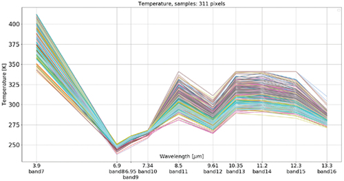
Figure 48. (a) Moderate Resolution Imaging Spectroradiometer (MODIS) image acquired on August 23, 2007, at 9.35 (CEST), covering Greece, depicted in false colors (monitor-typical channel R = MODIS band 6 in the Middle Infrared, channel G = MODIS band 2 in the Near Infrared, channel B = MODIS band 3 in the Visible Blue), spatial resolution: 1 km, radiometrically calibrated into top-of-atmosphere reflectance (TOARF) values, where an Environment for Visualizing Images (ENVI, by L3Harris Geospatial) standard histogram stretching was applied for visualization purposes. (b) Satellite Image Automatic Mapper (SIAM™)’s map of color names (Baraldi, Citation2017, Citation2019a; Baraldi et al., Citation2018a, Citation2018b, Citation2006; Baraldi & Tiede, Citation2018a, Citation2018b), generated from the MODIS image shown in (a), consisting of 83 spectral categories, depicted in pseudo-colors, refer to the SIAM map legend shown in and .
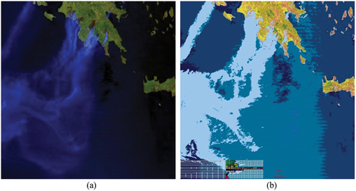
Figure 49. At left, portion of the image shown in , radiometrically calibrated into top-of-atmosphere reflectance (TOARF) values. Moderate Resolution Imaging Spectroradiometer (MODIS) image acquired on August 23, 2007, at 9.35 (CEST), covering Greece, depicted in false colors (monitor-typical channel R = MODIS band 6 in the Middle Infrared, channel G = MODIS band 2 in the Near Infrared, channel B = MODIS band 3 in the Visible Blue), spatial resolution: 1 km, radiometrically calibrated into top-of-atmosphere reflectance (TOARF) values, where an Environment for Visualizing Images (ENVI, by L3Harris Geospatial) standard histogram stretching was applied for visualization purposes. At right, Map Legend – Red: fire pixel detected in both the traditional MODIS Fire Detection (MOFID) algorithm and the SOIL MAPPER-based Fire Detection (SOMAFID) algorithm, an expert system for thermal anomalies detection (Pellegrini, Natali, & Baraldi, Citation2008). White: fire pixel detected by SOMAFID, exclusively. Green: fire pixel detected by MOFID, exclusively.
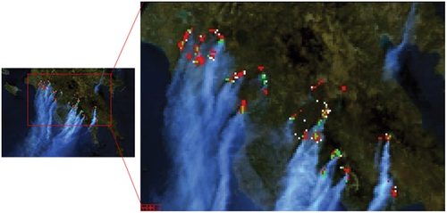
Figure 50. Legend (vocabulary) of hyperspectral color names adopted by the prior knowledge-based Landsat-like Satellite Image Automatic Mapper™ (L-SIAM™, release 88 version 7, see ) lightweight computer program for multi-spectral (MS) reflectance space hyperpolyhedralization (see Figures 29 and 30 in the Part 1), superpixel detection (see Figure 31 in the Part 1) and object-mean view (piecewise-constant input image approximation) quality assessment (Baraldi, Citation2017, Citation2019a; Baraldi et al., Citation2006, Citation2010a, Citation2010b, Citation2018a, Citation2018b; Baraldi & Tiede, Citation2018a, Citation2018b). Noteworthy, hyperspectral color names do not exist in human languages. Since humans employ a visible RGB imaging sensor as visual data source, human languages employ eleven basic color (BC) names, investigated by linguistics (Berlin & Kay, Citation1969), to partition an RGB data space into polyhedra, which are intuitive to think of and easy to visualize, see Figure 29 in the Part 1. On the contrary, hyperspectral color names (see Figure 30 in the Part 1) must be made up with (invented as) new words, not-yet existing in human languages, to be community-agreed upon for correct (conventional) interpretation before use by members of a community (refer to Subsection 4.2 in the Part 1). For the sake of representation compactness, pseudo-colors associated with the 96 color names/spectral categories, corresponding to a partition of the MS reflectance hyperspace into a discrete and finite ensemble of mutually exclusive and totally exhaustive hyperpolyhedra, equivalent to 96 envelopes/families of spectral signatures (see Figures 29 and 30 in the Part 1), are gathered along the same raw if they share the same parent spectral category (parent hyperpolyhedron) in the prior knowledge-based (static, non-adaptive to data) SIAM decision tree, e.g. “strong” vegetation, equivalent to a spectral end-member (Adams et al., Citation1995). The pseudo-color of a spectral category (color name) is chosen to mimic natural RGB colors of pixels belonging to that spectral category (Baraldi, Citation2017, Citation2019a; Baraldi et al., Citation2006, Citation2010a, Citation2010b, Citation2018a, Citation2018b; Baraldi & Tiede, Citation2018a, Citation2018b).
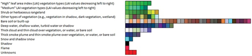
Figure 51. (a) False color quick-look Red-Green-Blue (RGB) Sentinel-2A Multi-Spectral Instrument (MSI) image Level-1C, calibrated into top-of-atmosphere reflectance (TOARF) values, depicting a surface area in SE Australia, acquired on 2019-12-31. In particular: R = Middle Infrared (MIR) = Band 11, G = Near Infrared (NIR) = Band 8, B = Visible Blue = Band 2. Spatial resolution: 10 m. No histogram stretching is applied for visualization purposes. (b) Same as Figure (a), followed by an Environment for Visualizing Images (ENVI, by L3Harris Geospatial) standard histogram stretching, applied for visualization purposes. (c) SIAM’s map of color names generated from Figure (a), consisting of 96 spectral categories (color names) depicted in pseudo-colors. Map of color names legend: 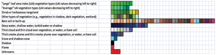
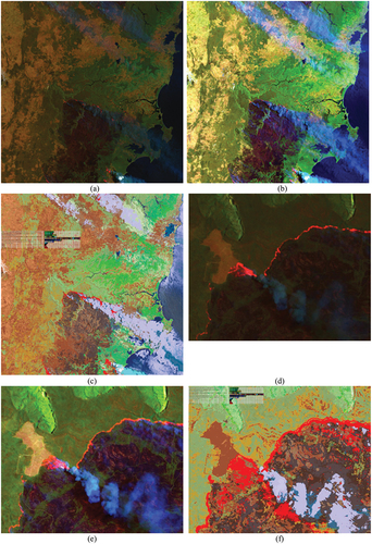
Figure 52. Multi-spectral (MS) signature in top-of-atmosphere reflectance (TOARF) values in range [0, 1], byte-coded into range {0, 255}, such that TOARF_byte = BYTE(TOARF_float * 255.0 + 0.5), where TOARF_byte ∈ {0, 255} is affected by a discretization (quantization) error = (TOARF_Max – TOARF_Min)/255 bins/2 (due to rounding to the closest integer, either above or below) = (1.0–0.0)/255.0/2.0 = 0.002 = 0.2%, to be considered negligible (Baraldi, Citation2017, Citation2019a; Baraldi et al., Citation2006, Citation2010a, Citation2010b, Citation2018a, Citation2018b; Baraldi & Tiede, Citation2018a, Citation2018b) (refer to Subsection 3.3.2 in the Part 1). (a) Active fire samples (region of interest, ROI), MS signature in TOARF_byte values in range {0, 255}, Sentinel-2A Multi-Spectral Instrument (MSI) image Level-1C, of Australia, acquired on 2019-12-31 and shown in , with bands 1 to 6 equivalent to Landsat-7 ETM+ bands 1 to 5 and 7, respectively. No thermal channel is available in Sentinel-2 MSI imagery, equivalent to the Landsat 7 ETM+ channels 61 and/or 62. (b) For comparison purposes with Figure (a), active fire samples, whose MS signature in TOARF_byte values belongs to range {0, 255}, are selected from a Landsat 7 ETM+ image of Senegal, Path: 203, Row: 051, acquisition date: 2001-01-11. Thermal band ETM62 in kelvin degrees in interval [−100, 155], linearly shifted into range {0, 255}. The two sensor-specific active fire spectral signatures in TOARF values shown in Figure (a) and Figure (b) should be compared with those collected by the geostationary GOES-16 ABI imaging sensor, shown in and .
![Figure 52. Multi-spectral (MS) signature in top-of-atmosphere reflectance (TOARF) values in range [0, 1], byte-coded into range {0, 255}, such that TOARF_byte = BYTE(TOARF_float * 255.0 + 0.5), where TOARF_byte ∈ {0, 255} is affected by a discretization (quantization) error = (TOARF_Max – TOARF_Min)/255 bins/2 (due to rounding to the closest integer, either above or below) = (1.0–0.0)/255.0/2.0 = 0.002 = 0.2%, to be considered negligible (Baraldi, Citation2017, Citation2019a; Baraldi et al., Citation2006, Citation2010a, Citation2010b, Citation2018a, Citation2018b; Baraldi & Tiede, Citation2018a, Citation2018b) (refer to Subsection 3.3.2 in the Part 1). (a) Active fire samples (region of interest, ROI), MS signature in TOARF_byte values in range {0, 255}, Sentinel-2A Multi-Spectral Instrument (MSI) image Level-1C, of Australia, acquired on 2019-12-31 and shown in Figure 51, with bands 1 to 6 equivalent to Landsat-7 ETM+ bands 1 to 5 and 7, respectively. No thermal channel is available in Sentinel-2 MSI imagery, equivalent to the Landsat 7 ETM+ channels 61 and/or 62. (b) For comparison purposes with Figure (a), active fire samples, whose MS signature in TOARF_byte values belongs to range {0, 255}, are selected from a Landsat 7 ETM+ image of Senegal, Path: 203, Row: 051, acquisition date: 2001-01-11. Thermal band ETM62 in kelvin degrees in interval [−100, 155], linearly shifted into range {0, 255}. The two sensor-specific active fire spectral signatures in TOARF values shown in Figure (a) and Figure (b) should be compared with those collected by the geostationary GOES-16 ABI imaging sensor, shown in Figures 46 and 47.](/cms/asset/51c644e8-a12a-42f6-9464-58ecd2c91320/tbed_a_2017582_f0008_c.jpg)
Figure 53. Ideal Earth observation (EO) optical sensory data-derived Level 2/Analysis Ready Data (ARD) product generation system design as a hierarchical alternating sequence of: (A) hybrid (combined deductive and inductive) class-conditional radiometric enhancement of EO Level 1 multi-spectral (MS) top-of-atmosphere reflectance (TOARF) values into EO Level 2/ARD surface reflectance (SURF) 1-of-3, SURF 2-of-3, SURF 3-of-3 and surface albedo values (EC – European Commission, Citation2020; Li et al., Citation2012; Malenovsky et al., Citation2007; Schaepman-Strub et al., Citation2006; Shuai et al., Citation2020) corrected in sequence for (1) atmospheric, (5) topographic (6) adjacency and (7) bidirectional reflectance distribution function (BRDF) effects (Egorov, Roy, Zhang, Hansen, & Kommareddy, Citation2018), and (B) hybrid (combined deductive and inductive) classification of TOARF, SURF 1-of-3 to SURF 3-of-3 and surface albedo values into a stepwise sequence of EO Level 2/ARD scene classification maps (SCMs), whose legend (taxonomy) of community-agreed land cover (LC) class names, in addition to quality layers Cloud and Cloud–shadow, increases stepwise in mapping accuracy and/or in semantics, i.e. stepwise, it reaches deeper semantic levels/finer semantic granularities in a hierarchical LC class taxonomy, see Figure 3 in the Part 1. An instantiation of this EO image pre-processing system design for EO Level 2/ARD symbolic and subsymbolic co-products generation is depicted in . In comparison with this desirable system design, the existing ESA Sen2Cor software system design (see Figure 38 in the Part 1) adopts no hierarchical alternating approach between MS image classification and MS image radiometric enhancement. In more detail, it accomplishes, first, one SCM generation from TOARF values based on a per-pixel (2D spatial context-insensitive) prior spectral knowledge-based decision-tree classifier (synonym for static/non-adaptive-to-data decision-tree for MS color naming, see Figures 29 and 30 in the Part 1). Next, in the ESA Sen2Cor workflow, a stratified/class-conditional MS image radiometric enhancement of TOARF into SURF 1-of-3 up to SURF 3-of-3 values corrected for atmospheric, topographic and adjacency effects is accomplished in sequence, stratified (class-conditioned) by (the haze map and cirrus map of) the same SCM product generated at first stage from TOARF values. In summary, the ESA Sen2Cor SCM co-product is TOARF-derived; hence, it is not “aligned” with data in the ESA Sen2Cor output MS image co-product, consisting of TOARF values radiometrically corrected into SURF 3-of-3 values (refer to Subsection 3.3.2 in the Part 1), where, typically, SURF ≠ TOARF holds, see Equation (9) in the Part 1.
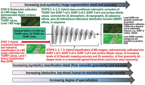
Figure 54. The well-known engineering principles of modularity, hierarchy and regularity, recommended for system scalability (Lipson, Citation2007), characterize a single-date EO optical image processing system design for state-of-the-art multi-sensor EO data-derived Level 2/Analysis Ready Data (ARD) product generation, encompassing an ARD-specific symbolic co-product, known as Scene Classification Map (SCM) (refer to Subsection 8.1.1), and an ARD-specific numerical co-product (refer to Subsection 8.1.2) to be estimated alternately and hierarchically, see . Stage 1: Absolute radiometric calibration (Cal) of dimensionless Digital Numbers (DNs) into top-of-atmosphere (TOA) radiance (TOARD) values ≥ 0. Stage 2: Cal of TOARD into TOA reflectance (TOARF) values ∈ [0.0, 1.0]. Stage 3: EO image classification by an automatic computer vision (CV) system, based on a convergence of spatial with colorimetric evidence (refer to Subsection 4.1 in the Part 1). Stage 4: Class-conditional/Stratified atmospheric correction of TOARF into surface reflectance (SURF) 1-of-3 values ∈ [0, 1]. Stage 5: Class-conditional/Stratified Topographic Correction (STRATCOR) of SURF 1-of-3 into SURF 2-of-3 values. Stage 6: Class-conditional/Stratified adjacency effect correction of SURF 2-of-3 into SURF 3-of-3 values. Stage 7: Class-conditional/Stratified bidirectional reflectance distribution function (BRDF) effect correction of SURF 3-of-3 values into surface albedo values (Bilal et al., Citation2019; EC – European Commission, Citation2020; Egorov, Roy, Zhang, Hansen, & Kommareddy, Citation2018; Franch et al., Citation2019; Li et al., Citation2012; Malenovsky et al., Citation2007; Qiu et al., Citation2019; Schaepman-Strub et al., Citation2006; Shuai et al., Citation2020). This original ARD system design is alternative to, for example, the EO image processing system design and implementation proposed in (Qiu et al., Citation2019) where, to augment the temporal consistency of USGS Landsat ARD imagery, neither topographic correction nor BRDF effect correction is land cover (LC) class-conditional. Worth mentioning, both SCM (referred to as land cover) and surface albedo (referred to as albedo) are included in the list of terrestrial Essential Climate Variables (ECVs) defined by the World Climate Organization (WCO) (Bojinski et al., Citation2014) (see Table 2 in the Part 1), which complies with the Group on Earth Observations (GEO)’s second implementation plan for years 2016–2025 of a new Global Earth Observation System of (component) Systems (GEOSS) as expert EO data-derived information and knowledge system (GEO – Group on Earth Observations, Citation2015; Nativi et al., Citation2015, Citation2020; Santoro et al., Citation2017), see Figure 1 in the Part 1.
![Figure 54. The well-known engineering principles of modularity, hierarchy and regularity, recommended for system scalability (Lipson, Citation2007), characterize a single-date EO optical image processing system design for state-of-the-art multi-sensor EO data-derived Level 2/Analysis Ready Data (ARD) product generation, encompassing an ARD-specific symbolic co-product, known as Scene Classification Map (SCM) (refer to Subsection 8.1.1), and an ARD-specific numerical co-product (refer to Subsection 8.1.2) to be estimated alternately and hierarchically, see Figure 53. Stage 1: Absolute radiometric calibration (Cal) of dimensionless Digital Numbers (DNs) into top-of-atmosphere (TOA) radiance (TOARD) values ≥ 0. Stage 2: Cal of TOARD into TOA reflectance (TOARF) values ∈ [0.0, 1.0]. Stage 3: EO image classification by an automatic computer vision (CV) system, based on a convergence of spatial with colorimetric evidence (refer to Subsection 4.1 in the Part 1). Stage 4: Class-conditional/Stratified atmospheric correction of TOARF into surface reflectance (SURF) 1-of-3 values ∈ [0, 1]. Stage 5: Class-conditional/Stratified Topographic Correction (STRATCOR) of SURF 1-of-3 into SURF 2-of-3 values. Stage 6: Class-conditional/Stratified adjacency effect correction of SURF 2-of-3 into SURF 3-of-3 values. Stage 7: Class-conditional/Stratified bidirectional reflectance distribution function (BRDF) effect correction of SURF 3-of-3 values into surface albedo values (Bilal et al., Citation2019; EC – European Commission, Citation2020; Egorov, Roy, Zhang, Hansen, & Kommareddy, Citation2018; Franch et al., Citation2019; Li et al., Citation2012; Malenovsky et al., Citation2007; Qiu et al., Citation2019; Schaepman-Strub et al., Citation2006; Shuai et al., Citation2020). This original ARD system design is alternative to, for example, the EO image processing system design and implementation proposed in (Qiu et al., Citation2019) where, to augment the temporal consistency of USGS Landsat ARD imagery, neither topographic correction nor BRDF effect correction is land cover (LC) class-conditional. Worth mentioning, both SCM (referred to as land cover) and surface albedo (referred to as albedo) are included in the list of terrestrial Essential Climate Variables (ECVs) defined by the World Climate Organization (WCO) (Bojinski et al., Citation2014) (see Table 2 in the Part 1), which complies with the Group on Earth Observations (GEO)’s second implementation plan for years 2016–2025 of a new Global Earth Observation System of (component) Systems (GEOSS) as expert EO data-derived information and knowledge system (GEO – Group on Earth Observations, Citation2015; Nativi et al., Citation2015, Citation2020; Santoro et al., Citation2017), see Figure 1 in the Part 1.](/cms/asset/e0975773-9d6d-4c18-a2da-1a711c614766/tbed_a_2017582_f0010_c.jpg)
Figure 55. Top left: Red-Green-Blue (RGB) image, source: Akiyoshi Kitaoka @AkiyoshiKitaoka, web page: http://nymag.com/selectall/2017/02/strawberries-look-red-without-red-pixels-color-constancy.html. Strawberries appear to be reddish, though the pixels are not, refer to the monitor-typical RGB input-output histograms shown at bottom left. No histogram stretching is applied for visualization purposes, see the monitor-typical RGB input-output histograms shown at bottom left. Top right: Output of the self-organizing statistical model-based color constancy algorithm, as reported in (Baraldi, Citation2017; Baraldi & Tiede, Citation2018a, Citation2018b; Baraldi et al., Citation2017; Vo et al., Citation2016), input with the image shown top left. No histogram stretching is applied for visualization purposes, see the monitor-typical RGB input-output histograms shown at bottom right.
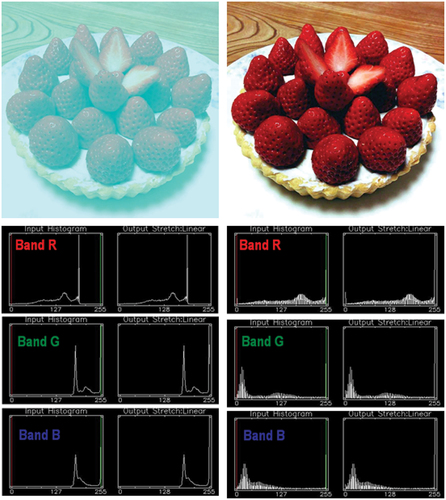
Figure 56. Fully automated two-stage stratified (class-conditional) topographic correction (STRATCOR) (Baraldi et al., Citation2010). (a) Zoomed area of a Landsat 7 ETM+ image of Colorado, USA (path: 128, row: 021, acquisition date: 2000–08-09), depicted in false colors (R: band ETM5, G: band ETM4, B: band ETM1), 30 m resolution, radiometrically calibrated into TOARF values. (b) STRATCOR applied to the Landsat image shown at left, with data stratification based on the Shuttle Radar Topography Mission (SRTM) Digital Elevation Model (DEM) and a 18-class preliminary spectral map generated at coarse granularity by the 7-band Landsat-like Satellite Image Automatic Mapper (L-SIAM) software toolbox (Baraldi, Citation2017, Citation2019a; Baraldi et al., Citation2006, Citation2010a, Citation2010b, Citation2018a, Citation2018b; Baraldi & Tiede, Citation2018a, Citation2018b), see .
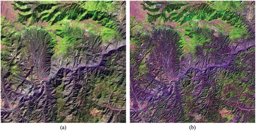
Figure 57. (a) Meteosat Second Generation (MSG) Spinning Enhanced Visible and InfraRed Imager (SEVIRI) image acquired on 2012-05-30, radiometrically calibrated into TOARF values and depicted in false colors (R: band MIR, G: band NIR, B: band Blue), spatial resolution: 3 km. No histogram stretching is applied for visualization purposes. (b). Advanced Very High Resolution Radiometer (AVHRR)-like SIAM (AV-SIAM™, release 88 version 7) hyperpolyhedralization of the MS reflectance hyperspace and prior knowledge-based mapping of the input MS image into a vocabulary of hypercolor names. The AV-SIAM map legend, consisting of 83 spectral categories (see ), is depicted in pseudo-colors, similar to those shown in : 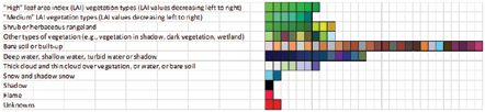
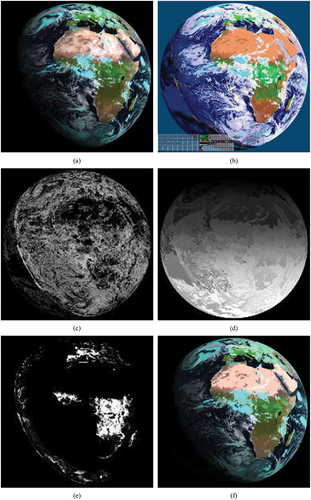
Figure 58. (a) Airborne 10 cm resolution true-color Red-Green-Blue (RGB) orthophoto of Trento, Italy, 4017 × 4096 pixels in size x 3 bands, acquired in 2014 and provided with no radiometric calibration metadata file. No histogram stretching is applied for visualization purposes. (b) Same RGB orthophoto, subject to self-organizing statistical color constancy (Baraldi, Citation2017; Baraldi & Tiede, Citation2018a, Citation2018b; Baraldi et al., Citation2017; Vo et al., Citation2016). No histogram stretching is applied for visualization purposes. (c) RGBIAM’s polyhedralization of the RGB color space and prior knowledge-based map of RGB color names generated from the RGB image, pre-processed by a color constancy algorithm (Baraldi, Citation2017; Baraldi & Tiede, Citation2018a, Citation2018b; Baraldi et al., Citation2017; Vo et al., Citation2016). The RGBIAM legend of RGB color names, consisting of 50 spectral categories at fine discretization granularity, is depicted in pseudo-colors. Map legend, shown in : 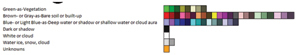
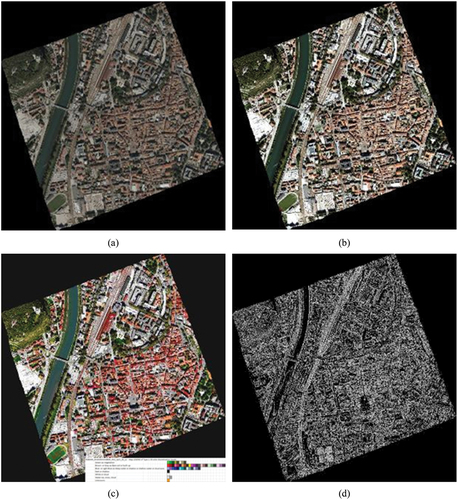
Figure 59. Legend (vocabulary) of RGB color names adopted by the prior knowledge-based Red-Green-Blue (RGB) Image Automatic Mapper™ (RGBIAM™, release 6 version 2) lightweight computer program for RGB data space polyhedralization (see Figure 29 in the Part 1), superpixel detection (see Figure 31 in the Part 1) and object-mean view (piecewise-constant input image approximation) quality assessment (Baraldi, Citation2017, Citation2019a; Baraldi et al., Citation2006; Citation2018a, Citation2018b; Baraldi & Tiede, Citation2018a, Citation2018b). Before running RGBIAM to map onto a deterministic RGB color name each pixel value of an input 3-band RGB image, encoded in either true- or false-colors, the RGB image should be pre-processed (enhanced) for normalization/ harmonization/ calibration (Cal) purposes, e.g. by means of a color constancy algorithm (Baraldi, Citation2017; Baraldi & Tiede, Citation2018a, Citation2018b; Baraldi et al., Citation2017; Boynton, Citation1990; Finlayson et al., Citation2001; Gevers et al., Citation2012; Gijsenij et al., Citation2010; Vo et al., Citation2016), see and . The RGBIAM implementation (release 6 version 2) adopts 12 basic color (BC) names (polyhedra) as coarse RGB color space partitioning, consisting of the eleven BC names adopted by human languages (Berlin & Kay, Citation1969), specifically, black, white, gray, red, orange, yellow, green, blue, purple, pink and brown (refer to Subsection 4.2 in the Part 1), plus category “Unknowns” (refer to Section 2 in the Part 1), and 50 color names as fine color quantization (discretization) granularity, featuring parent-child relationships from the coarse to the fine quantization level. For the sake of representation compactness, pseudo-colors associated with the 50 color names (spectral categories, corresponding to a mutually exclusive and totally exhaustive partition of the RGB data space into polyhedra, see Figure 29 in the Part 1) are gathered along the same raw if they share the same parent spectral category (parent polyhedron) in the prior knowledge-based (static, non-adaptive to data) RGBIAM decision tree. The pseudo-color of a spectral category (color name) is chosen to mimic natural RGB colors of pixels belonging to that spectral category (Baraldi, Citation2017; Baraldi & Tiede, Citation2018a, Citation2018b; Baraldi et al., Citation2017; Vo et al., Citation2016).
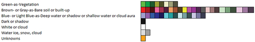
Figure 60. First test image of a Cambodia site (Baraldi & Tiede, Citation2018b). Final 3-level Cloud/Cloud–shadow/Others maps generated by the three algorithms under comparison, specifically, single-date AutoCloud+, the single-date AutoCloud+ Baraldi & Tiede, Citation2018a, Citation2018b), the single-date Sen2Cor (DLR - Deutsches Zentrum für Luft-und Raumfahrt e.V. and VEGA Technologies, Citation2011; ESA - European Space Agency, Citation2015) and the multi-date MAJA (Hagolle et al., Citation2017; Main-Knorn et al., Citation2018), where class “Others” is overlaid with the input Sentinel-2 A Multi-Spectral Instrument (MSI) Level 1C image, radiometrically calibrated into top-of-atmosphere reflectance (TOARF) values and depicted in false-colors: monitor-typical Red-Green-Blue (RGB) channels are selected as R = Near Infrared (NIR) channel, G = Visible Red channel, B = Visible Green channel. Histogram stretching is applied for visualization purposes. Output class Cloud is shown in a green pseudo-color, class Cloud–shadow in a yellow pseudo-color.
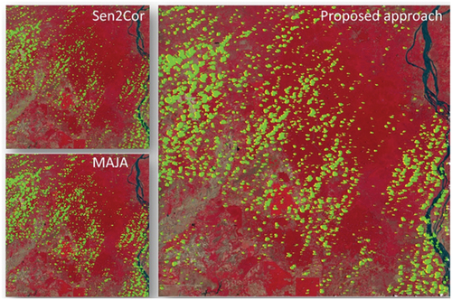
Figure 61. First test image of a Cambodia site (Baraldi & Tiede, Citation2018b). Zoom-in of the final 3-level Cloud/Cloud–shadow/Others maps generated by the three algorithms under comparison, where class “others” is overlaid with the input Sentinel-2 A Multi-Spectral Instrument (MSI) Level 1C image, radiometrically calibrated into top-of-atmosphere (TOA) reflectance (TOARF) values and depicted in false-colors: monitor-typical RGB channels are selected as R = Near InfraRed (NIR) channel, G = Visible Red channel, B = Visible Green channel. Histogram stretching is applied for visualization purposes. Output class Cloud is shown in a green pseudo-color, class Cloud–shadow in a yellow pseudo-color. Based on qualitative photointerpetation, the single-date Sen2Cor algorithm (DLR - Deutsches Zentrum für Luft-und Raumfahrt e.V. and VEGA Technologies, Citation2011; ESA - European Space Agency, Citation2015) appears to underestimate Cloud–shadows, although some Water areas are misclassified as Cloud–shadow. In addition, some River/river beds are misclassified as Cloud. These two cases of Cloud false positives and Cloud–shadow false positives are highlighted in blue circles. The multi-date MAJA algorithm (Hagolle et al., Citation2017; Main-Knorn et al., Citation2018), overlooks some Cloud instances small in size (in relative terms), as highlighted in red circles.
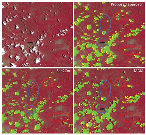
Figure 62. First test image of a Cambodia site (Baraldi & Tiede, Citation2018b). Extra zoom-in of the final 3-level Cloud/Cloud–shadow/Others maps generated by the three algorithms under comparison, where class “Others” is overlaid with the input Sentinel-2 A Multi-Spectral Instrument (MSI) Level 1C image, radiometrically calibrated into top-of-atmosphere (TOA) reflectance (TOARF) values and depicted in false-colors: monitor-typical RGB channels are selected as R = Near InfraRed (NIR) channel, G = Visible Red channel, B = Visible Green channel. Histogram stretching is applied for visualization purposes. Output class Cloud is shown in a green pseudo-color, class Cloud–shadow in a yellow pseudo-color. Based on qualitative photointerpetation, the single-date Sen2Cor algorithm (DLR - Deutsches Zentrum für Luft-und Raumfahrt e.V. and VEGA Technologies, Citation2011; ESA - European Space Agency, Citation2015) appears to underestimate class Cloud–shadow, although some detected Cloud–shadow instances are false positives because of misclassified Water areas. In addition, some River/river beds are misclassified as Cloud. To reduce false positives in Cloud–shadow detection, MAJA adopts a multi-date approach. Nevertheless, the multi-date MAJA algorithm (Hagolle et al., Citation2017; Main-Knorn et al., Citation2018), misses some instances of Cloud-over-water. Overall, MAJA’s Cloud and Cloud–shadow results look more “blocky” (affected by artifacts in localizing true boundaries of target image-objects).
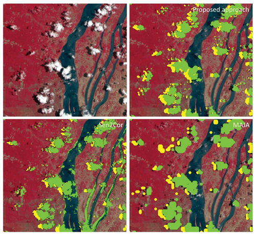
Figure 63. Typical values of a minimally dependent maximally informative (mDMI) set of outcome and process quantitative quality indicators (OP-Q2Is) featured by a pixel-based (2D spatial context-insensitive) 1D image analysis algorithm (see Figure 18 in the Part 1) for Cloud and Cloud-shadow detection in MS imagery (see Figure 22 in the Part 1), such as Fmask (Zhu et al., Citation2015), ESA Sen2Cor (DLR – Deutsches Zentrum für Luft-und Raumfahrt e.V. and VEGA Technologies, Citation2011; ESA – European Space Agency, Citation2015) and CNES-DLR MAJA (Hagolle et al., Citation2017; Main-Knorn et al., Citation2018) (see ), considered a mandatory EO image understanding (classification) task for quality layers detection in Analysis Ready Data (ARD) workflows.
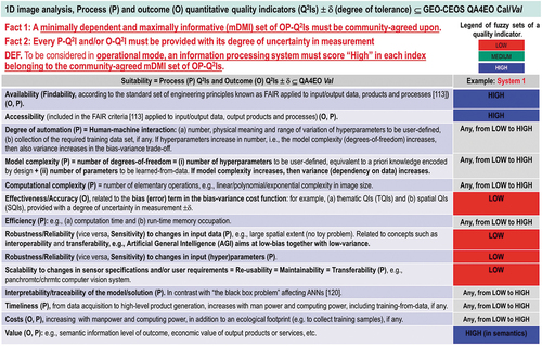
Figure 64. Typical values of a minimally dependent maximally informative (mDMI) set of outcome and process quantitative quality indicators (OP-Q2Is) featured by a deep convolutional neural network (DCNN) (Cimpoi et al., Citation2014) involved with Cloud and Cloud-shadow detection in MS imagery (Bartoš, Citation2017; EOportal, Citation2020; Wieland et al., Citation2019) (see ), considered a mandatory EO image understanding (classification) task for quality layers detection in Analysis Ready Data (ARD) workflows.
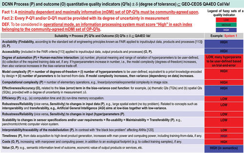
Figure 65. Expected values of a minimally dependent maximally informative (mDMI) set of outcome and process quantitative quality indicators (OP-Q2Is) featured by a “universal” multi-sensor automatic AutoCloud+ algorithm for Cloud and Cloud-shadow detection in multi-spectral (MS) imagery (Baraldi & Tiede, Citation2018a, Citation2018b) (see ), considered a mandatory EO image understanding (classification) task for quality layers detection in Analysis Ready Data (ARD) workflows. By scoring “high” in each indicator of an mDMI set of OP-Q2Is, a “universal” multi-sensor automated AutoCloud+ algorithm for Cloud and Cloud-shadow quality layers detection in MS imagery is expected to be considered in operational mode (Baraldi, Citation2017; Baraldi & Tiede, Citation2018a, Citation2018b), as necessary-but-not-sufficient precondition of ARD workflows.
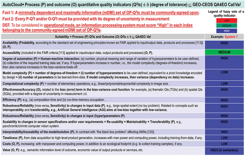
Table 4. The Satellite Image Automatic Mapper™ (SIAM™) lightweight computer program (release 88 version 7) for multi-spectral (MS) reflectance space hyperpolyhedralization (see Figures 29 and 30 in the Part 1), superpixel detection (see Figure 31 in the Part 1) and object-mean view quality assessment (Baraldi, Citation2017, Citation2019a; Baraldi et al., Citation2006, Citation2010a, Citation2010b, Citation2018a, Citation2018b; Baraldi & Tiede, Citation2018a, Citation2018b). SIAM is an Earth observation (EO) system of systems scalable to any past, present or future MS imaging sensor, provided with radiometric calibration metadata parameters for radiometric calibration (Cal) of digital numbers into top-of-atmosphere reflectance (TOARF), surface reflectance (SURF) or surface albedo values, where relationship ‘TOARF ⊇ SURF ⊇ Surface albedo’ = Equation (8) in the Part 1 holds. SIAM is an expert system (deductive/ top-down/ prior knowledge-based static decision tree, non-adaptive to input data) for mapping each color value in the MS reflectance space into a color name belonging to the SIAM vocabulary of hypercolor names. It consists of the following subsystems. (i) 7-band Landsat-like SIAM™ (L-SIAM™), with Landsat-like input channels Blue (B) = Blue0.45÷0.50, Green (G) = Green0.54÷0.58, Red (R) = Red0.65÷0.68, Near Infrared (NIR) = NIR0.78÷0.90, Middle Infrared 1 (MIR1) = MIR1.57÷1.65, Middle Infrared 2 (MIR2) = MIR2.08÷2.35, and Thermal Infrared (TIR) = TIR10.4–12.5, see Figure 7 and Table 3 in the Part 1. (ii) 4-band (channels G, R, NIR, MIR1) SPOT-like SIAM™ (S-SIAM™). (iii) 4-band (channels R, NIR, MIR1, and TIR) Advanced Very High Resolution Radiometer (AVHRR)-like SIAM™ (AV-SIAM™). (iv) 4-band (channels B, G, R, and NIR) QuickBird-like SIAM™ (Q-SIAM™) (Baraldi, Citation2017, Citation2019a; Baraldi et al., Citation2006, Citation2010a, Citation2010b, Citation2018a, Citation2018b; Baraldi & Tiede, Citation2018a, Citation2018b).
Table 5. Conceptual/methodological comparison of existing algorithms for Cloud and Cloud-shadow quality layers detection in spaceborne MS imagery for EO Level 2/ARD-specific symbolic output co-product generation.
The preceding Part 1 (Baraldi et al., Citation2022) of the present Part 2 is provided with a relevant survey value in the multi-disciplinary domain of cognitive science (Ball, Citation2021; Capra & Luisi, Citation2014; Hassabis, Kumaran, Summerfield, & Botvinick, Citation2017; Hoffman, Citation2008, Citation2014; Langley, Citation2012; Miller, Citation2003; Mindfire Foundation, Citation2018; Mitchell, Citation2019; Parisi, Citation1991; Santoro, Lampinen, Mathewson, Lillicrap, & Raposo, Citation2021; Serra & Zanarini, Citation1990; Varela, Thompson, & Rosch, Citation1991; Wikipedia, Citation2019), encompassing disciplines like philosophy (Capurro & Hjørland, Citation2003; Dreyfus, Citation1965, Citation1991, Citation1992; Fjelland, Citation2020; Fodor, Citation1998; Peirce, Citation1994), semiotics (Ball, Citation2021; Peirce, Citation1994; Perez, Citation2020, Citation2021; Salad, Citation2019; Santoro et al., Citation2021; Wikipedia, Citation2021e), linguistics (Ball, Citation2021; Berlin & Kay, Citation1969; Firth, Citation1962; Rescorla, Citation2019; Saba, Citation2020a, Citation2020c), anthropology (Harari, Citation2011, Citation2017; Wikipedia, Citation2019), neuroscience (Barrett, Citation2017; Buonomano, Citation2018; Cepelewicz, Citation2021; Daniels, Citation2021; Hathaway, Citation2021; Hawkins, Citation2021; Hawkins, Ahmad, & Cui, Citation2017; Kaufman, Churchland, & Ryu et al., Citation2014; Kosslyn, Citation1994; Libby & Buschman, Citation2021; Mason & Kandel, Citation1991; Salinas, Citation2021a, Citation2021b; Slotnick, Thompson, & Kosslyn, Citation2005; Zador, Citation2019), which is focused on the study of the brain machinery in the mind-brain problem (Hassabis et al., Citation2017; Hoffman, Citation2008; Serra & Zanarini, Citation1990; Westphal, Citation2016), computational neuroscience (Beniaguev, Segev, & London, Citation2021; DiCarlo, Citation2017; Gidon et al., Citation2020; Heitger, Rosenthaler, von der Heydt, Peterhans, & Kubler, Citation1992; Pessoa, Citation1996; Rodrigues & du Buf, Citation2009), psychophysics (Benavente, Vanrell, & Baldrich, Citation2008; Bowers & Davis, Citation2012; Griffin, Citation2006; Lähteenlahti, Citation2021; Mermillod, Bugaiska, & Bonin, Citation2013; Parraga, Benavente, Vanrell, & Baldrich, Citation2009; Vecera & Farah, Citation1997), psychology (APS, Citation2008; Hehe, Citation2021), computer science, formal logic (Laurini & Thompson, Citation1992; Sowa, Citation2000), mathematics, physics, statistics and (the meta-science of) engineering (Langley, Citation2012; Santoro et al., Citation2021; Wikipedia, Citation2019), which includes knowledge engineering (Laurini & Thompson, Citation1992) and geographic information science (GIScience) (Buyong, Citation2007; Couclelis, Citation2010, Citation2012; Ferreira, Camara, & Monteiro, Citation2014; Fonseca, Egenhofer, Agouris, & Camara, Citation2002; Goodchild, Yuan, & Cova, Citation2007; Hitzler et al., Citation2012; Hu, Citation2017; Kuhn, Citation2005; Longley, Goodchild, Maguire, & Rhind, Citation2005; Maciel et al., Citation2018; Sheth, Citation2015; Sonka, Hlavac, & Boyle, Citation1994; Stock, Hobona, Granell, & Jackson, Citation2011). In the preceding Part 1, the multi-disciplinary domain of cognitive science is regarded as background knowledge of the remote sensing (RS) meta-science (science of sciences) community (Baraldi, Citation2017; Baraldi & Tiede, Citation2018a, Citation2018b; Couclelis, Citation2012), see Figure 11(a) in the Part 1.
In agreement with the intergovernmental Group on Earth Observations (GEO)-Committee on Earth Observation Satellites (CEOS) Quality Assurance Framework for Earth Observation (QA4EO) Calibration/Validation (Cal/Val) requirements (Baraldi, Citation2009, Citation2017, Citation2019b; Baraldi, Humber, Tiede, & Lang, Citation2018a, Citation2018b; Baraldi & Tiede, Citation2018a, Citation2018b; GEO-CEOS, Citation2010; Schaepman-Strub, Schaepman, Painter, Dangel, & Martonchik, Citation2006; Shuai et al., Citation2020) (refer to Section 2 in the Part 1), overarching goal of the RS meta-science is to transform multi-source Earth observation (EO) big sensory data, characterized by the six Vs of volume, variety, veracity, velocity, volatility and value (Metternicht, Mueller, & Lucas, Citation2020), into value-adding information products and services (VAPS) in operational mode, suitable for coping with the United Nations (UN) Sustainable Development Goals (SDGs) from year 2015 to 2030 (UN, Citation2021), at regional to global spatial extents, in a new era of Space Economy 4.0 (Mazzucato & Robinson, Citation2017), see Figure 10 in the Part 1.
In 2017, a new notion of Space Economy 4.0 was proposed by Mazzucato and Robinson to the European Space Agency (ESA) (Mazzucato & Robinson, Citation2017). According to these authors, in the “seamless innovation chain” required by a new Space Economy 4.0 (see Figure 10 in the Part 1), first-stage “horizontal” (enabling) capacity building, coping with background conditions necessary to specialization, is preliminary to second-stage “vertical” (deep and narrow, specialized) policies, suitable for coping with a potentially huge worldwide market of institutional and private end-users of space technology, encompassing grand societal challenges, such as the UN SDGs from year 2015 to 2030 (UN – United Nations, Department of Economic and Social Affairs, Citation2021).
In the preceding Part 1, the first original contribution is formalization of semantic relationship
‘Deep Convolutional Neural Network (DCNN) ⊂ Deep Learning-from-data (DL) ⊂ Machine Learning-from-data (ML) → Artificial Weak/Narrow Intelligence (ANI) → Artificial General/Strong Intelligence (AGI) ⊃ Computer Vision (CV) ⊃ Earth Observation Image Understanding (EO-IU) ⊃ Analysis Ready Data (ARD)’ = Eq. (5) in the Part 1,
where semantic relationship ‘ARD ⊂ EO-IU ⊂ CV ⊂ AGI ⊂ Cognitive science’ = Eq. (3) in the Part 1 holds (see Figure 11(a) in the Part 1), while ANI is formulated as
‘ANI = [DCNN ⊂ DL ⊂ ML logical-OR Traditional deductive Artificial Intelligence (static expert systems, non-adaptive to data, also known as Good Old-Fashioned Artificial Intelligence, GOFAI)]’ = Eq. (6) in the Part 1.
In these semantic relationships, adopted herein as working hypotheses (postulates, axioms), symbol ‘→’ denotes semantic relationship part-of (without inheritance), pointing from the supplier to the client, not to be confused with semantic relationship subset-of, ‘⊃’, meaning specialization with inheritance from the superset (at left) to the subset (at right), in agreement with symbols adopted by the standard Unified Modeling Language (UML) for graphical modeling of object-oriented software (Fowler, Citation2003), see Figure 11(a) and Figure 11(b) in the Part 1.
In these original equations, buzzword “Artificial Intelligence”, increasingly adopted by the scientific community together with the general public in recent years, is disambiguated into the two better-constrained (better-defined, to be better understood) notions of ANI and AGI, where ANI = Equation (6) in the Part 1 is regarded as part-without-inheritance-of AGI, such that semantic relationship ‘AGI ← ANI ← ML ⊃ DL ⊃ DCNN’ = Equation (5) in the Part 1 holds, in agreement with the notions of AGI ≠ ANI increasingly promoted by relevant portions of the existing literature (Bills, Citation2020; Chollet, Citation2019; Dreyfus, Citation1965, Citation1991, Citation1992; EC, Citation2019; Fjelland, Citation2020; Hassabis et al., Citation2017; Ideami, Citation2021; Jajal, Citation2018; Jordan, Citation2018; Mindfire Foundation, Citation2018; Mitchell, Citation2021; Practical AI, Citation2020; Saba, Citation2020c; Santoro et al., Citation2021; Sweeney, Citation2018a; Thompson, Citation2018; Wolski, Citation2020a, Citation2020b; Zawadzki, Citation2021).
Worth mentioning, AGI = Equation (5) and ANI = Equation (6) in the Part 1 are inconsistent with (alternative to) relationship (Claire, Citation2019; Copeland, Citation2016)
‘A(G/N)I ⊃ ML ⊃ DL ⊃ DCNN’ = Equation (7) in the Part 1,
adopted as postulate by increasing portions of the ML, CV and RS meta-sciences in recent years, see Figure 11(c) in the Part 1. For example, in (Copeland, Citation2016), it is reported that: “since an early flush of optimism in the 1950s, smaller subsets of Artificial Intelligence – first machine learning, then deep learning, a subset of machine learning – have created even larger disruptions.” Moreover, starting from 2012, when the ‘DCNN ⊂ DL ⊂ ML’ paradigm was successfully proposed by the CV community (Krizhevsky, Sutskever, & Hinton, Citation2012), DL enthusiasts, practitioners and scientists have been promoting DL as synonym for A(G/N)I (Claire, Citation2019; Copeland, Citation2016), see Figure 11(c) in the Part 1.
Alternative to Equation (7) in the Part 1, the two semantic relationships adopted herein as working hypotheses, specifically, AGI = Equation (5) and ANI = Equation (6) in the Part 1, are endorsed by the European Commission (EC), when it acknowledges (at least in words) that “currently deployed Artificial Intelligence systems are examples of ANI” (EC – European Commission, Citation2019), in agreement with relevant portions of the scientific literature (Bills, Citation2020; Chollet, Citation2019; Dreyfus, Citation1965, Citation1991, Citation1992; Fjelland, Citation2020; Hassabis et al., Citation2017; Ideami, Citation2021; Jajal, Citation2018; Jordan, Citation2018; Mindfire Foundation, Citation2018; Practical AI, Citation2020; Romero, Citation2021; Santoro et al., Citation2021; Sweeney, Citation2018a; Wolski, Citation2020a, Citation2020b; Zawadzki, Citation2021).
Moreover, in spite of its recent popularity, Equation (7) in the Part 1 is in contrast with the early days of the ML meta-science, when scientists never confused ML with A(G/N)I, i.e. relationship ‘ML ⊂ A(G/N)I’ was never promoted (Bishop, Citation1995; Cherkassky & Mulier, Citation1998; Geman, Bienenstock, & Doursat, Citation1992; Mahadevan, Citation2019; Russell & Norvig, Citation1995; Wolpert, Citation1996; Wolpert & Macready, Citation1997).
Increasing disillusionment on ‘DL ⊂ ML → ANI → AGI’ mainly stems from portions of the ML community (Bartoš, Citation2017; Bills, Citation2020; Bourdakos, Citation2017; Brendel, Citation2019; Brendel & Bethge, Citation2019; Chollet, Citation2019; Crawford & Paglen, Citation2019; Daniels, Citation2021; Deutsch, Citation2012; Dreyfus, Citation1965, Citation1991, Citation1992; Etzioni, Citation2017; Expert.ai, Citation2020; Fjelland, Citation2020; Geman et al., Citation1992; Gonfalonieri, Citation2020; Hao, Citation2019; Hassabis et al., Citation2017; Hawkins, Citation2021; Ideami, Citation2021; Jordan, Citation2018; Langley, Citation2012; LeVine, Citation2017; Lohr, Citation2018; Lukianoff, Citation2019; Mahadevan, Citation2019; Marcus, Citation2018, Citation2020; Marks, Citation2021; Mindfire Foundation, Citation2018; Mitchell, Citation2019, Citation2021; Nguyen, Yosinski, & Clune, Citation2014; Pearl & Mackenzie, Citation2018; Peng, Citation2017; Perez, Citation2017; Pfeffer, Citation2018; Practical AI, Citation2020; Rahimi, Citation2017; Romero, Citation2021; Russell & Norvig, Citation1995; Saba, Citation2020c; Santoro et al., Citation2021; Strubell, Ganesh, & McCallum, Citation2019; Sweeney, Citation2018a, Citation2018b; Szegedy et al., Citation2013; Thompson, Citation2018; U.S. DARPA, Citation2018; Wolpert, Citation1996; Wolpert & Macready, Citation1997; Wolski, Citation2020a, Citation2020b; Ye, Citation2020; Yuille and Chenxi Liu, Citation2019; Zador, Citation2019) pre-dating the recent hype on DL (Claire, Citation2019; Copeland, Citation2016; Krizhevsky et al., Citation2012).
For the sake of completeness, in contrast with the recent popularity of Equation (7) in the Part 1, Appendix I of the Part 1 presents a few quotes of interest in the multi-disciplinary domain of cognitive science, by Alberto Romero (Romero, Citation2021), Walid Saba (Saba, Citation2020c), Michael Jordan (Jordan, Citation2018), Oren Etzioni (Etzioni, Citation2017), Stuart Russell (Bills, Citation2020; Practical AI, Citation2020), Pat Langley (Langley, Citation2012), EC (EC – European Commission, Citation2019), Melanie Mitchell (Mitchell, Citation2019), Geoffrey Hinton (LeVine, Citation2017), Ali Rahimi (Pfeffer, Citation2018; Rahimi, Citation2017), Maciej Wolski (Wolski, Citation2020a, Citation2020b) and Karen Hao (Hao, Citation2019; Strubell et al., Citation2019). Unfortunately, these critical contributions have been largely ignored, to date, by meta-sciences like engineering and RS, where Artificial Intelligence is typically coped with as a problem in statistics, see Equation (7) in the Part 1.
In Figure 11(a) of the Part 1, semantic relationship
‘ARD ⊂ EO-IU ⊂ CV ⊂ AGI ⊂ Cognitive science’ = Equation (3) in the Part 1
holds. In line with this semantic relationship, EO image (2D gridded data)-derived ARD generation is not regarded as a data pre-processing task, suitable for data enhancement preliminary to data processing (analysis). In data pre-processing (enhancement), an input numerical variable, either sensory data or sensory data-derived, is transformed into an output numerical variable of augmented quality (e.g. radiometric quality, geometric quality, etc.), somehow more useful, hence, considered more informative. Intuitively, quality enhancement of a numerical variable pertains to the problem domain of quantitative/unequivocal information-as-thing (Capurro & Hjørland, Citation2003), typical of the Shannon data communication/transmission theory (Baraldi, Citation2017; Baraldi et al., Citation2018a, Citation2018b; Baraldi & Tiede, Citation2018a, Citation2018b; Capurro & Hjørland, Citation2003; Santoro et al., Citation2021; Sarkar, Citation2018; Shannon, Citation1948) (refer to Subsection 3.3.3 in the Part 1).
Rather, the aforementioned Equation (3) in the Part 1 regards EO image (2D gridded data)-derived ARD generation as a cognitive problem in the CV sub-domain of cognitive science, see Figure 11(a) in the Part 1.
Encompassing both CV and biological vision (DiCarlo, Citation2017; Dubey, Agrawal, Pathak, Griffiths, & Efros, Citation2018; Heitger et al., Citation1992; Kosslyn, Citation1994; Marr, Citation1982; Mason & Kandel, Citation1991; Mély, Linsley, & Serre, Citation2018; Öğmen & Herzog, Citation2010; Perez, Citation2018; Pessoa, Citation1996; Piasini et al., Citation2021; Rappe, Citation2018; Rodrigues & du Buf, Citation2009; Slotnick et al., Citation2005; Vecera & Farah, Citation1997; Victor, Citation1994), the notion of vision is synonym for inherently ill-posed scene-from-image reconstruction and understanding (Baraldi, Citation2017; Baraldi & Tiede, Citation2018a, Citation2018b; Matsuyama & Hwang, Citation1990), see Figure 20 in the Part 1. Vision is a cognitive task (refer to Subsection 4.1 in the Part 1), pertaining to the problem domain of inherently ill-posed/ qualitative/ equivocal information-as-data-interpretation tasks (Capurro & Hjørland, Citation2003) (refer to Subsection 3.3.3 in the Part 1), which are typically investigated by disciplines like philosophy (Capurro & Hjørland, Citation2003; Dreyfus, Citation1965, Citation1991, Citation1992; Fjelland, Citation2020; Fodor, Citation1998; Peirce, Citation1994), semiotics (Ball, Citation2021; Peirce, Citation1994; Perez, Citation2020, Citation2021; Salad, Citation2019; Santoro et al., Citation2021; Wikipedia, Citation2021e) and linguistics (Ball, Citation2021; Berlin & Kay, Citation1969; Firth, Citation1962; Rescorla, Citation2019; Saba, Citation2020a, Citation2020c), encompassed by the multi-disciplinary domain of cognitive science, see Figure 11(a) in the Part 1.
In quantitative data analysis of scientific quality, sensory data/numerical variables must be better constrained, to be better behaved and better understood, than data typically employed in qualitative data analysis, which is inherently subjective, not-replicable, like in artworks.
Proposed by the RS meta-science community in recent years (CEOS, Citation2018; Dwyer et al., Citation2018; Helder et al., Citation2018; NASA, Citation2019; Qiu et al., Citation2019; USGS – U.S. Geological Survey, Citation2018a, Citation2018c), the notion of ARD aims at enabling expert and non-expert end-users to access/retrieve EO big data ready for use in quantitative data analysis of scientific quality, without requiring laborious EO data pre-processing for geometric and radiometric data enhancement, preliminary to EO data processing (analysis, interpretation) (Dwyer et al., Citation2018). For example, in the ensemble of alternative EO optical image-derived Level 2/ARD product definitions and software implementations existing to date (CEOS – Committee on Earth Observation Satellites, Citation2018; Dwyer et al., Citation2018; Gómez-Chova, Camps-Valls, Calpe-Maravilla, Guanter, & Moreno, Citation2007; Helder et al., Citation2018; Houborga & McCabe, Citation2018; NASA – National Aeronautics and Space Administration, Citation2019; OHB, Citation2016; Tiede, Sudmanns, Augustin, & Baraldi, Citation2020; Tiede, Sudmanns, Augustin, & Baraldi, Citation2021; USGS, Citation2018a, Citation2018b; USGS – U.S. Geological Survey, Citation2018c; Vermote & Saleous, Citation2007) (see Figures 35 and 36 in the Part 1), Cloud and Cloud-shadow quality layers (strata, masks) are typically considered necessary to model data uncertainty in EO optical imagery to be considered suitable for quantitative data analysis of scientific quality.
In contrast with the ARD policy of pursuing multi-source EO data-through-time harmonization/ standardization/ interoperability in support of scholarly/scientific digital data understanding (GO FAIR, Citation2021; ISO/EIC, Citation2015; Wikipedia, Citation2018; Wilkinson, Dumontier, Aalbersberg et al., Citation2016), a popular example of qualitative data analysis of non-scientific quality, equivalent to subjective not-replicable artworks, is provided by the Google Earth Engine Timelapse application (ESA, Citation2021; Google Earth Engine, Citation2021), showing videos of multi-year time-series of spaceborne multi-sensor EO optical images whose radiometric quality, if any, is heterogeneous/non-harmonized. In practice, the Google Earth Engine Timelapse application is suitable for gaining a “wow” effect in qualitative human photointerpretation exclusively, equivalent to manmade works of art. Unfortunately, it is completely inadequate for quantitative big data analysis of scientific quality, which would require a (super) human-level ‘EO-IU ⊂ CV ⊂ AGI’ system in operational mode, which does not exist yet (refer to Section 2 in the Part 1), suitable for coping with the six Vs of big data (Metternicht et al., Citation2020) involved with multi-sensor EO big 2D gridded data interpretation tasks.
The potential impact of the cognitive problem of ‘ARD ⊂ EO-IU ⊂ CV ⊂ AGI’ on the RS community is highlighted by recalling here that the notion of ARD has been strictly coupled with the concept of EO (raster-based) data cube, proposed as innovative midstream EO technology by the RS community in recent years (Open Data Cube, Citation2020; Baumann, Citation2017; CEOS, Citation2020; Giuliani et al., Citation2017; Giuliani, Chatenoux, Piller, Moser, & Lacroix, Citation2020; Lewis et al., Citation2017; Strobl et al., Citation2017).
Synonym for EO (raster-based) big data cube in the 4D geospace-time physical world-domain, Digital (Twin) Earth is yet-another buzzword of increasing popularity (Craglia et al., Citation2012; Goodchild, Citation1999; Gore, Citation1999; Guo, Goodchild, & Annoni, Citation2020; ISDE, Citation2012; Loekken, Le Saux, & Aparicio, Citation2020; Metternicht et al., Citation2020), stemming from Al Gore’s 1998 insight that “we need a Digital Earth, a multi-resolution, 3D representation of the planet, into which we can embed vast quantities of geo-referenced data” (Craglia et al., Citation2012; Gore, Citation1999; Loekken et al., Citation2020). A Digital (Twin) Earth is “an interactive digital replica of the entire planet that can facilitate a shared understanding of the multiple relationships between the physical and natural environments and society” (Guo & Annoni, Citation2020). It is the pre-dating concept of Digital Twin of a complex system, defined as “a set of virtual information constructs that fully describes a potential or actual physical system from the micro atomic level to the macro geometrical level” (Grieves & Vickers, Citation2017), applied to planet Earth (Loekken et al., Citation2020).
Unfortunately, a community-agreed definition of EO (raster-based) data cube does not exist yet, although several recommendations and implementations have been made (Open Data Cube, Citation2020; Baumann, Citation2017; CEOS – Committee on Earth Observation Satellites, Citation2020; Giuliani et al., Citation2017, Citation2020; Lewis et al., Citation2017; Strobl et al., Citation2017). A community-agreed definition of ARD, to be adopted as standard baseline in EO data cube implementations, does not exist either. As a consequence, in common practice, many EO (raster-based) data cube definitions and implementations do not require ARD and, vice versa, an ever-increasing ensemble of new (supposedly better) ARD definitions and/or ARD-specific software implementations is proposed by the RS community, independently of a standardized/harmonized definition of EO big data cube (refer to Section 2 in the Part 1).
To foster innovation across the global value chain required by a new notion of Space Economy 4.0 (Mazzucato & Robinson, Citation2017) (see Figure 10 in the Part 1), the second original contribution of the Part 1, preliminary to the present Part 2, is to promote system interoperability/ standardization/ harmonization, encompassing third-level semantic/ontological interoperability (refer to Section 2 in the Part 1), among existing EO optical sensory image-derived Level 2/ARD product definitions and software implementations (see Figures 35 and 36 in the Part 1), while overcoming their limitations, investigated at the Marr five levels of understanding of an information processing system.
In short, the Marr five levels of understanding of an information processing system are identified as follows (Baraldi, Citation2017; Baraldi et al., Citation2018a, Citation2018b; Baraldi & Tiede, Citation2018a, Citation2018b; Marr, Citation1982; Quinlan, Citation2012; Sonka et al., Citation1994) (refer to Subsection 3.2 in the Part 1).
(i) Outcome and process requirements specification.
(ii) Information/knowledge representation.
(iii) System design (architecture).
(iv) Algorithm.
(v) Implementation.
Noteworthy, among the five Marr levels of system understanding, the three more abstract levels, namely, outcome and process requirements specification, information/knowledge representation and system design, are typically considered the linchpin of success of an information processing system, rather than algorithm and implementation (Baraldi, Citation2017; Baraldi et al., Citation2018a, Citation2018b; Baraldi & Tiede, Citation2018a, Citation2018b; Marr, Citation1982; Quinlan, Citation2012; Sonka et al., Citation1994) (refer to Subsection 3.2 in the Part 1). Although based on commonsense knowledge (Etzioni, Citation2017; Expert.ai, Citation2020; Thompson, Citation2018; U.S. DARPA – Defense Advanced Research Projects Agency, Citation2018; Wikipedia, Citation2021c) (refer to Section 2 in the Part 1), this observation (true-fact) is oversighted in large portions of the RS and CV literature, where ‘CV ⊃ EO-IU ⊃ ARD’ system analysis, assessment and inter-comparison are typically focused on algorithm and implementation, e.g. refer to works like (Foga et al., Citation2017) and (Ghosh & Kaabouch, Citation2014) as negative examples not to be imitated in the inter-comparison of CV systems.
To be achieved across existing EO optical sensory image-derived Level 2/ARD product definitions and software implementations (see Figures 35 and 36 in the Part 1), the pursuit of interoperability/ standardization/ harmonization, encompassing third-level semantic/ontological interoperability (refer to Section 2 in the Part 1), is a cognitive (information-as-data-interpretation) task (see Equation (3) in the Part 1), inherently ill-posed in the Hadamard sense (Hadamard, Citation1902), which requires Bayesian constraints (Bowers & Davis, Citation2012; Ghahramani, Citation2011; Hunt & Tyrrell, Citation2012; Lähteenlahti, Citation2021; Quinlan, Citation2012; Sarkar, Citation2018) to become better posed for numerical solution (Baraldi, Citation2017; Baraldi et al., Citation2018a, Citation2018b; Baraldi & Tiede, Citation2018a, Citation2018b; Bishop, Citation1995; Cherkassky & Mulier, Citation1998; Dubey et al., Citation2018) (refer to Section 2 in the Part 1). Constraints adopted in the Part 1 are standard product and process quality criteria, selected from the existing literature. They are summarized as follows.
The popular Findable Accessible Interoperable and Reusable (FAIR) guiding principles for scholarly/scientific digital data and non-data (e.g. analytical pipelines) management (GO FAIR – International Support and Coordination Office, Citation2021; Wilkinson, Dumontier, Aalbersberg et al., Citation2016), see Table 1 in the Part 1. Accounting for the fundamental difference between outcome (product, e.g. sensory data-derived product) and process, it is worth observing that term reusability in the FAIR data principles (see Table 1 in the Part 1) is conceptually equivalent to tenet regularity adopted by the popular engineering principles of structured (data processing) system design, encompassing modularity, hierarchy and regularity (Lipson, Citation2007), considered neither necessary nor sufficient, but highly recommended for system scalability (Page-Jones, Citation1988). Term interoperability in the FAIR data principles (see Table 1 in the Part 1) becomes, in the process domain, the tenet of system interoperability. It is typically defined as “the ability of systems to provide services to and accept services from other systems and to use the services so exchanged to enable them to operate effectively together” (Wikipedia, Citation2018). According to (ISO/IEC, Citation2015), system (functional unit) interoperability is “the capability to communicate, execute programs, or transfer data among various functional units [systems] in a manner that requires the user to have little or no knowledge of the unique characteristics of those units”; in short, it is “the capability of two or more functional units [systems] to process data cooperatively”. In more detail, there are three levels of system interoperability (opposite of heterogeneity), corresponding to three generations of information processing systems (Sheth, Citation2015; Wikipedia, Citation2018), reported hereafter for the sake of completeness (refer to Section 2 in the Part 1).
First lexical/communication level of system interoperability, involving computer system and data communication protocols, data types and formats, operating systems, transparency of location, distribution and replication of data, etc. (Sheth, Citation2015; Wikipedia, Citation2018).
Second syntax/structural level of system interoperability. “Syntactic interoperability only focuses on the technical ability of systems to exchange data” (Hitzler et al., Citation2012). Intuitively, it is related to form, not content. According to Yingjie Hu, the term syntactics is in contrast with “the term semantics, which refers to the meaning of expressions in a language” (Hu, Citation2017). Syntactic interoperability of component systems involves the two Marr levels of abstraction of an information processing system known as information/knowledge representation and structured system design (architecture) (Baraldi, Citation2017; Baraldi et al., Citation2018a, Citation2018b; Baraldi & Tiede, Citation2018a, Citation2018b; Marr, Citation1982; Quinlan, Citation2012; Sonka et al., Citation1994) (refer to Subsection 3.2 in the Part 1), query languages and interfaces, etc. (Sheth, Citation2015; Wikipedia, Citation2018).
Third semantic/ontological level of system interoperability, increasingly domain-specific (Baraldi, Citation2017; Baraldi & Tiede, Citation2018a, Citation2018b; Bittner, Donnelly, & Winter, Citation2005; Green, Bean, & Myaeng, Citation2002; Hitzler et al., Citation2012; Hu, Citation2017; Kuhn, Citation2005; Laurini & Thompson, Citation1992; Matsuyama & Hwang, Citation1990; Nativi et al., Citation2015; Nativi, Santoro, Giuliani, & Mazzetti, Citation2020; Obrst, Whittaker, & Meng, Citation1999; Sheth, Citation2015; Sonka et al., Citation1994; Sowa, Citation2000; Stock et al., Citation2011; Wikipedia, Citation2018).
The visionary goal of the intergovernmental GEO’s implementation plan for years 2005–2015 of a Global Earth Observation System of (component) Systems (GEOSS) (EC and GEO, Citation2014; GEO, Citation2005, Citation2019; Mavridis, Citation2011), unaccomplished to date (GEO, Citation2015; Nativi et al., Citation2015, Citation2020; Santoro, Nativi, Maso, & Jirka, Citation2017), see Figure 1 in the Part 1. In 2014, GEO expressed the utmost recommendation that, for the next 10 years 2016–2025 (GEO – Group on Earth Observations, Citation2015), the second mandate of GEOSS is to evolve from an EO big data sharing infrastructure, intuitively referred to as data-centric approach (Nativi et al., Citation2020), to an expert EO data-derived information and knowledge system (Nativi et al., Citation2015, pp. 7, 22), intuitively referred to as knowledge-driven approach (Nativi et al., Citation2020), capable of supporting decision-making by successfully coping with challenges along all six community-agreed degrees (dimensionalities, axes) of complexity of big data (Guo, Goodchild, & Annoni, Citation2020, p. 1), known as the six Vs of volume, variety, veracity, velocity, volatility and value (Metternicht et al., Citation2020). The ongoing GEO activity on the identification, formalization and use of Essential (Community) Variables and related instances (see Table 2 in the Part 1) contributes to the process of making GEOSS an expert EO sensory data-derived information and knowledge system, capable of EO sensory data interpretation/transformation into Essential (Community) Variables in support of decision making (Nativi et al., Citation2015, p. 18, Citation2020; Santoro et al., Citation2017). It means that only high-level Essential (Community) Variables, rather than low-level EO big sensory data, should be delivered by GEOSS to end-users of spaceborne/airborne EO technologies for decision-making purposes. Focusing on the delivery to end-users of EO sensory data-derived Essential (Community) Variables as information sets relevant for decision-making (Santoro et al., Citation2017), in place of delivering low-level EO big sensory data, would reduce the Big Data requirements of the GEOSS digital Common Infrastructure (Nativi et al., Citation2015, p. 21, Citation2020) (see Figure 1 in the Part 1), in agreement with the increasingly popular Data-Information-Knowledge-Wisdom (DIKW) conceptual hierarchy where, typically, information is defined in terms of data, knowledge in terms of information and wisdom in terms of knowledge (Rowley, Citation2007; Rowley & Hartley, Citation2008; Wikipedia, Citation2020; Zeleny, Citation1987, Citation2005; Zins, Citation2007), see Figures 12 and 16 in the Part 1.
The ambitious, but realistic goals of the GEO-CEOS QA4EO Cal/Val guidelines (refer to references listed in this Section above). According to the intergovernmental GEO-CEOS QA4EO Cal/Val guidelines, the following requirements hold.
Timely, operational and comprehensive transformation of multi-sensor EO big sensory data into VAPS requires joint multi-objective optimization of: (a) Suitability, which implies Availability, Findability and Accessibility of product and/or process, together with (jointly with) product accuracy, process efficiency, process robustness to changes in input data, process robustness to changes in input hyperparameters to be user-defined based on heuristics, process transferability, process scalability, process interpretability, product and process cost in manpower, product and process cost in computer power, etc. (refer to Section 2 in the Part 1), and (b) Feasibility, synonym for viability/ practicality/ doableness (refer to Section 2 in the Part 1).
Each step in a data processing workflow must be validated, by an independent third party (GEO-CEOS, Citation2015), for quantitative quality assurance (QA)/quality traceability (vice versa, for error propagation and backtracking), where quality and/or error estimates must be provided with a degree of uncertainty in measurement. Synonym for error (uncertainty) propagation through an information processing chain, the general-purpose garbage in, garbage out (GIGO) principle is intuitive to deal with (Baraldi, Citation2017; Geiger et al., Citation2021; Thompson, Citation2018). Its formal version is the process of uncertainty estimation, based on a combination of the propagation law of uncertainty with the mathematical model of causality for the input-output data mapping (data link) at hand (Ma, Jia, Schaepman, & Zhao, Citation2020), according to the Guide to the Expression of Uncertainty in Measurement (JCGM, Citation2008) and the International Vocabulary of Metrology (JCGM, Citation2012) criteria issued by the Joint Committee for Guides in Metrology. Unfortunately, the large majority of works published in the RS literature presents outcome and process (OP) quantitative quality indicators (Q2Is) estimates, such as statistical estimates of thematic Q2Is (T-Q2Is), provided with no degree of uncertainty in measurement, ±δ (Lunetta & Elvidge, Citation1999). It is important to stress that OP-Q2Is published in the RS literature featuring no uncertainty estimate, ±δ, are in contrast with the principles of statistics (GEO-CEOS – Group on Earth Observations and Committee on Earth Observation Satellites, Citation2010; Holdgraf, Citation2013; JCGM – Joint Committee for Guides in Metrology, Citation2012; JCGM – Joint Committee for Guides in Metrology., Citation2008; Lunetta & Elvidge, Citation1999), i.e. they do not feature any statistical meaning (Baraldi, Citation2017; Baraldi, Boschetti, & Humber, Citation2014; Baraldi & Tiede, Citation2018a, Citation2018b). If this observation holds true as premise, then another fact holds true as consequence: since large portions of OP-Q2Is published in the RS literature feature no degree of uncertainty in measurement, ±δ, in disagreement with intergovernmental GEO-CEOS QA4EO Val requirements (GEO-CEOS – Group on Earth Observations and Committee on Earth Observation Satellites, Citation2010), then the statistical quality of a large portion of outcomes and/or processes published in the RS literature remains unknown to date (refer to Subsection 3.1 in the Part 1).
In the RS meta-science domain (Couclelis, Citation2012) (see Figure 11(a) in the Part 1), radiometric Cal (refer to Section 2 in the Part 1) is the process of transforming EO sensory data, typically encoded as non-negative dimensionless digital numbers (DNs, with DN ≥ 0) provided with no physical meaning at EO Level 0, into a physical variable, i.e. a numerical variable provided with a community-agreed radiometric unit of measure (Baraldi, Citation2009, Citation2017; Baraldi et al., Citation2018a, Citation2018b; Baraldi & Tiede, Citation2018a, Citation2018b; DigitalGlobe, Citation2017; EC - European Commission, Citation2020; GEO-CEOS – Group on Earth Observations and Committee on Earth Observation Satellites, Citation2010; Malenovsky et al., Citation2007; Pacifici, Longbotham, & Emery, Citation2014; Schaepman-Strub et al., Citation2006; Shuai et al., Citation2020), such as top-of-atmosphere radiance (TOARD) values, with TOARD ≥ 0, top-of-atmosphere reflectance (TOARF) values belonging to the physical domain of change [0.0, 1.0], surface reflectance (SURF) values in the physical range of change [0.0, 1.0] and surface albedo values in the physical range [0.0, 1.0]. Noteworthy, surface albedo is included (referred to as albedo) in the list of terrestrial Essential Climate Variables (ECVs) defined by the World Climate Organization (WCO) (Bojinski et al., Citation2014) (see Table 2 in the Part 1), which complies with requirements of the GEO second implementation plan for years 2016-2025 of a new GEOSS, regarded as expert EO data-derived information and knowledge system (GEO - Group on Earth Observations, Citation2015; Nativi et al., Citation2015, Citation2020; Santoro et al., Citation2017) (see Figure 1 in the Part 1), in agreement with the well-known DIKW hierarchical conceptualization (refer to references listed in this Section above), see Figures 12 and 16 in the Part 1. Intuitively, any (calibrated) physical variable, provided with a physical meaning, a physical unit of measure and a physical range of change, is better behaved and better understood than uncalibrated data (Baraldi, Citation2009; Pacifici et al., Citation2014). In particular, calibrated data can be input to:
Deductive/physical model-based inference systems (traditional static if-then decision trees, non-adaptive to data, known as expert systems) (Bishop, Citation1995; Cherkassky & Mulier, Citation1998; Laurini & Thompson, Citation1992; Sonka et al., Citation1994), often referred to as Good Old-Fashioned Artificial Intelligence (GOFAI) (Dreyfus, Citation1965, Citation1991, Citation1992; Santoro et al., Citation2021)
Inductive/statistical model-based inference systems (Laurini & Thompson, Citation1992; Peirce, Citation1994; Salmon, Citation1963). As well as
Hybrid (combined deductive and inductive) inference systems (Baraldi, Citation2017; Baraldi & Tiede, Citation2018a, Citation2018b; Bishop, Citation1995; Cherkassky & Mulier, Citation1998; Chomsky, Citation1957; Expert.ai, Citation2020; Hassabis et al., Citation2017; Laurini & Thompson, Citation1992; Liang, Citation2004; Marcus, Citation2018, Citation2020; Matsuyama & Hwang, Citation1990; Mindfire Foundation, Citation2018; Nagao & Matsuyama, Citation1980; Parisi, Citation1991; Piaget, Citation1970; Sonka et al., Citation1994; Sweeney, Citation2018b; Thompson, Citation2018; Zador, Citation2019), encompassed by AGI solutions in the multi-disciplinary domain of cognitive science, see Figure 11(a) in the Part 1.
In general, statistical model-based systems can be input with either uncalibrated or calibrated data, i.e. they do not require as input numerical variables provided with a physical meaning. Nevertheless, when input with calibrated data, which are better behaved than uncalibrated data, then statistical model-based systems typically gain in accuracy, robustness, transferability and scalability (refer to Subsection 3.1 in the Part 1).
Moreover, EO sensory data radiometrically calibrated into either TOARF, SURF or surface albedo values, all belonging to the physical range of change [0.0, 1.0], can be encoded as unsigned byte, affected by a negligible quantization error of 0.2% (refer to Subsection 3.3.2 in the Part 1). This property is largely oversighted by the RS community to date, because EO Level 1 TOARF values and Level 2/ARD SURF values are typically encoded as 16-bit unsigned short integer, such as in the Planet Surface Reflectance Product (Planet, Citation2019), the U.S. Landsat ARD format (Dwyer et al., Citation2018; Helder et al., Citation2018; NASA - National Aeronautics and Space Administration, Citation2019; USGS - U.S. Geological Survey, Citation2018a, Citation2018c) and the Level 1 TOARF and Level 2 SURF value formats adopted by the ground segment of the Italian Space Agency (ASI) Hyperspectral Precursor and Application Mission (PRISMA) (ASI, Citation2020; OHB, Citation2016). These multi-source EO big data archives, calibrated into TOARF or SURF values and encoded as 16-bit unsigned short integer, can be seamlessly transcoded into an 8-bit unsigned char, affected by a quantization error as low as 0.2%, with a 50% save in memory storage.
In line with this commonsense knowledge (Etzioni, Citation2017; Expert.ai, Citation2020; Thompson, Citation2018; U.S. DARPA - Defense Advanced Research Projects Agency, Citation2018; Wikipedia, Citation2021c) (refer to Section 2 in the Part 1), in the RS meta-science domain, to better cope with the six Vs of EO big data, namely, volume, variety, veracity, velocity, volatility and value (Metternicht et al., Citation2020), radiometric Cal of EO data is considered mandatory by the intergovernmental GEO-CEOS QA4EO Cal guidelines (refer to references listed in this Section above) (refer to Subsection 3.3.2 in the Part 1).
In spite of the aforementioned advantages of EO calibrated over uncalibrated data, it is enigmatic that, in the RS literature and in the RS common practice, EO data radiometric Cal is largely oversighted to date, although it is considered a well-known “prerequisite for physical model-based analysis of airborne and satellite sensor measurements in the optical domain” (Schaepman-Strub, Schaepman, Painter, Dangel and Martonchik, Citation2006), in compliance with the intergovernmental GEO-CEOS QA4EO Cal requirements (refer to references listed in this Section above). For example, in a survey of EO image classification systems published in the RS literature in year 2014 (Ghosh and Kaabouch, Citation2014), word “calibration” is absent and radiometric Cal tasks are totally ignored. Moreover, in the RS common practice, commercial or free-of-cost EO data processing software toolboxes typically consist of overly complicated collections (libraries) of inductive/statistical model-based ML-from-data algorithms to choose from based on heuristics (trial-and-error) (L3Harris Geospatial, Citation2009; OpenCV, 2020), which require as input no data radiometrically calibrated to be provided with a physical unit of radiometric measure (Baraldi, Citation2009; Baraldi, Citation2017; Baraldi & Boschetti, Citation2012a; Baraldi & Boschetti, Citation2012b; Baraldi, Boschetti, & Humber, Citation2014; Pacifici, Longbotham, & Emery, Citation2014), although statistical data analysis can benefit, in general, from better behaved calibrated data as input (refer to Subsection 3.3.2 in the Part 1).
Multi-objective optimization of an original minimally dependent and maximally informative (mDMI) set of OP-Q2Is (Baraldi, Citation2017; Baraldi & Boschetti, Citation2012a, Citation2012b; Baraldi et al., Citation2014, Citation2018a, Citation2018b; Baraldi & Tiede, Citation2018a, Citation2018b), proposed and instantiated to be community-agreed upon (refer to Subsection 3.1 in the Part 1). This is in contrast with a large portion of the RS literature, where the sole EO data mapping (e.g. classification) accuracy is typically adopted as “universal” scalar Q2I, in spite of the fact that, first, no “universal” scalar Q2I can exist in general, due to the non-injective property of Q2Is of complex phenomena, meaning that different instantiations of a target complex phenomenon (no toy problem) may feature the same scalar Q2I value (Baraldi, Citation2009, Citation2017). Second, no product (outcome) Q2I, identified herein as O-Q2I, such as an EO data mapping accuracy measure, provides any insight on the quality of the data mapping process and vice versa, i.e. no process Q2I, identified herein as P-Q2I, provides any insight on the quality of the outcome.
According to the Pareto formal analysis of multi-objective optimization problems, optimization of an mDMI set of OP-Q2Is is an inherently ill-posed problem in the Hadamard sense (Hadamard, Citation1902), where many Pareto optimal solutions lying on the Pareto efficient frontier can be considered equally good (Boschetti, Flasse, & Brivio, Citation2004), to be chosen from based on heuristics (empirical criteria, trial-and-error) (refer to Section 2 in the Part 1). For example, any ‘AGI ⊃ CV ⊃ EO-IU ⊃ ARD’ system solution lying on the Pareto efficient frontier can be considered in operational mode, which means it is eligible for dealing with the six Vs of volume, variety, veracity, velocity, volatility and value featured by geospatial-temporal EO big data (Metternicht et al., Citation2020).
Selected from the RS literature (Baraldi, Citation2017; Baraldi & Boschetti, Citation2012a, Citation2012b; Baraldi et al., Citation2014, Citation2018a, Citation2018b; Baraldi & Tiede, Citation2018a, Citation2018b) and adopted by Section 2 in the Part 1, the following definition is reported herein, for the sake of completeness.
An information processing system, such as an ‘AGI ⊃ CV ⊃ EO-IU ⊃ ARD’ system (see Figure 11(a) in the Part 1), is considered in operational mode if and only if it scores (fuzzy) “high” (Zadeh, Citation1965) in each Q2I belonging to an mDMI set of OP-Q2Is (such as that instantiated in Subsection 3.1 of the Part 1), to be community-agreed upon.
The third original contribution of the Part 1 is to propose a novel semantics-enriched ARD product-pair (outcome, O) and process (P) gold standard, eligible for third-level semantic/ontological interoperability (refer to this Section above), regarded as “horizontal” (enabling) general-purpose application- and user-independent AGI for EO (AGI4EO) technology in a new notion of Space Economy 4.0 (Mazzucato & Robinson, Citation2017), see Figure 10 in the Part 1. Coping with background conditions necessary to specialization in a new era of Space Economy 4.0 (Mazzucato & Robinson, Citation2017), an innovative semantics-enriched ARD product-pair and process gold standard is required to be accomplished in operational mode (refer to the definition provided in this Section above) at the space segment, in an AGI for space segment (AGI4Space) research and technological development (RTD) framework (see Figure 10 in the Part 1), and/or at the midstream segment, in an AGI for Data and Information Access Services (AGI4DIAS) RTD framework (see Figure 10 in the Part 1), by both private and public EO big data providers (refer to Section 2 in the Part 1).
Regarded in past years as planned future developments in intelligent EO satellites (Zhou, Citation2001), ongoing RTD initiatives about AGI4Space applications are reported in recent works (EOportal, Citation2020; ESA, Citation2019; Esposito et al., Citation2019a, Citation2019b; GISCafe News, Citation2018), in compliance with a new notion of Space Economy 4.0, see Figure 10 in the Part 1. For example, in (GISCafe News, Citation2018), it is reported that “the Earth-i led consortium will develop a number of new Earth Observation technologies that will enable processes, such as the enhancement of image resolution, cloud-detection, change detection and video compression, to take place on-board a small satellite (Satellite Applications Catapult, Citation2018) rather than on the ground. This will accelerate the delivery of high-quality images, video and information-rich analytics to end-users. On-board cloud detection will make the tasking of satellites more efficient and increase the probability of capturing a usable and useful image or video. To achieve these goals, ‘Project OVERPaSS‘ will implement, test and demonstrate very high-resolution optical image analysis techniques, involving both new software and dedicated hardware installed onboard small satellites to radically increase their ability to process data in space. The project will also determine the extent to which these capabilities could be routinely deployed on-board British optical imaging satellites in the future” (refer to Subsection 5.1 in the Part 1).
The fourth original contribution of the Part 1 is to consider availability of an innovative semantics-enriched ‘ARD ⊂ EO-IU ⊂ CV ⊂ AGI’ system in operational mode at the space segment and/or midstream segment, where ARD-specific product and process suitability (encompassing accuracy, findability, accessibility, interoperability, reusability, cost, etc.), together with feasibility (doableness, practicality, viability), are jointly maximized, in compliance with a community-agreed mDMI set of OP-Q2Is (see Subsection 3.1 in the Part 1), with the GEO-CEOS QA4EO Cal/Val requirements (refer to references listed in this Section above) and with the FAIR guiding principles for scholarly/scientific digital data and non-data (e.g. analytical pipelines) management (refer to references listed in this Section above) (see Table 1 in the Part 1). Availability of an innovative semantics-enriched ‘ARD ⊂ EO-IU ⊂ CV ⊂ AGI’ system, implemented in operational mode at the space segment and/or midstream segment, is regarded as:
Necessary-but-not-sufficient precondition of the RS community for developing a “horizontal” (enabling) AGI4DIAS infrastructure at the midstream = ‘AGI-enabled DIAS = Semantics-enabled DIAS 2.0 (DIAS 2nd generation) = AGI + DIAS 1.0 + Semantic content-based image retrieval (SCBIR) + Semantics-enabled information/knowledge discovery (SEIKD)’ = Equation (1) in the Part 1, suitable for augmenting the findable and accessible factors of the FAIR guiding principles for scientific data (product and process) management (GO FAIR – International Support and Coordination Office, Citation2021; Wilkinson, Dumontier, Aalbersberg et al., Citation2016), see Table 1 in the Part 1.
Necessary-but-not-sufficient precondition of the downstream segment for developing an ever-increasing ensemble of “vertical” (deep and narrow, specialized) domain- and user-specific VAPS in operational mode, available for use by a potentially huge worldwide market of institutional and private end-users of space technology, encompassing the UN SDGs at global scale, see Figure 10 in the Part 1.
In summary, the previous Part 1 of the present Part 2 identifies as linchpin for success of a new Space Economy 4.0 an innovative semantics-enriched ARD product-pair and process gold standard, which is:
(a) required to be accomplished in operational mode, at the space segment (in an AGI4Space framework) and/or midstream segment (in an AGI4DIAS framework), by both public and private EO big data providers, and
(b) considered both a conceptual and a tangible boundary between a “horizontal” enabling first phase at the midstream segment and a “vertical” specialization (deep and narrow) second phase at the downstream segment, see Figure 10 in the Part 1.
Starting from takeaways about an innovative semantics-enriched ARD product-pair and process gold standard, proposed in Subsection 5.2 of the Part 1, the overarching goal of the present Part 2 is instantiation of an innovative semantics-enriched ARD product-pair (outcome, O) and process (P), eligible for consideration as reference standard, to be investigated at the Marr five levels of system understanding (refer to references listed in this Section above), ranging from product and process requirements specification to software implementation, in the pursuit of suitability together with feasibility, in compliance with the mDMI set of OP-Q2Is proposed in Subsection 3.1 of the Part 1 (refer to references listed in this Section above), which includes the popular FAIR quality criteria for scientific data (product and process) management (refer to references listed in this Section above) and complies with the GEO-CEOS QA4EO Cal/Val guidelines (refer to references listed in this Section above).
Let us consider two examples of how present initiatives of space agencies, like ESA, aiming at the development of operational, comprehensive and timely multi-source EO data-derived VAPS in support of the UN SDGs, would benefit from the proposed ‘ARD ⊂ EO-IU ⊂ CV ⊂ AGI’ system availability in operational mode at the space segment and/or midstream segment (see Figure 10 in the Part 1), in order to augment their score in an mDMI set of OP-Q2Is, such as that proposed in Subsection 3.1 of the Part 1.
In 2014, ESA started the EO Thematic Exploitation Platforms (TEPs) initiative, a set of RTD activities whose first phase (up to 2017) aimed at creating an ecosystem of interconnected TEPs on European footing, addressing the following themes of EO data applications (ESA, Citation2020c): Coastal, Forestry, Hydrology, Geohazards, Polar, Urban themes; and Food Security (refer to Section 2 in the Part 1).
In addition to the ESA TEPs, the ongoing ESA Climate Change Initiative’s parallel projects (ESA, Citation2017b, Citation2020a, Citation2020b) aim at realizing the full potential of the long-term global EO data archives that ESA together with its Member states have established over the last thirty years, as a significant and timely contribution to the ECV databases required by the WCO and the United Nations Framework Convention on Climate Change (Bojinski et al., Citation2014), see Table 2 in the Part 1. The ESA Climate Change Initiative ensures that full capital is derived from past, ongoing and planned ESA missions, relevant ESA-managed archives of Third-Party Mission data and the Copernicus Sentinel constellation (ESA – European Space Agency, Citation2020a, Citation2020b). With this aim, the ESA Climate Change Initiative consists of parallel projects, geared to ECV data production, including the following (ESA – European Space Agency, Citation2020a): Aerosol, Biomass, Cloud, Fire (ESA – European Space Agency, Citation2020b), Green house gases, Glaciers, Antarctic ice sheet, Greenland Ice sheet, Land cover (ESA – European Space Agency, Citation2017b), High resolution land cover, Lakes, Land surface temperature, Ocean colour, Ozone, Permafrost, REgional Carbon Cycle Assessment and Processes’ phase 2, Sea surface salinity, Sea ice, Sea level, Seal level budget closure, Sea state, Snow, Soil moisture, Sea surface temperature and Water vapour (refer to Section 2 in the Part 1).
Unfortunately, existing ESA TEPs and the ESA Climate Change Initiative are parallel projects lacking inter-platform operability, in contrast with the first principles of a new Space Economy 4.0 (Mazzucato & Robinson, Citation2017). In practice, each of these ESA EO big data processing chains specializes from the start, instead of starting a “vertical” user- and domain-specific specialization/competition second stage following a “horizontal” (enabling) harmonized/ interoperable/ cooperative EO data processing first stage, encompassing the RTD of a general-purpose user- and application-independent multi-source Level 2/ARD product generation (CEOS – Committee on Earth Observation Satellites, Citation2018; DLR and VEGA, Citation2011; Dwyer et al., Citation2018; ESA, Citation2015; Gómez-Chova et al., Citation2007; Helder et al., Citation2018; Houborga & McCabe, Citation2018; NASA – National Aeronautics and Space Administration, Citation2019; OHB, Citation2016; USGS – U.S. Geological Survey, Citation2018a, Citation2018b, Citation2018c; Vermote & Saleous, Citation2007), in combination with a harmonized/interoperable EO ARD cube management system (Open Data Cube, Citation2020; Baumann, Citation2017; CEOS – Committee on Earth Observation Satellites, Citation2020; Giuliani et al., Citation2017, Citation2020; Lewis et al., Citation2017; Strobl et al., Citation2017).
Because the present Part 2 of this two-part paper is subsequent to the Part 1 proposed in (Baraldi et al., Citation2022), to ease the understanding of the conceptual relationships between topics dealt with by sections located within and across the two paper parts, a numbered list is provided below as summary of content of the two-part paper.
Our original problem description, opportunity recognition and working project’s secondary and primary objectives are presented in Section 2 of the Part 1. Problem identification and opportunity recognition: How increasingly popular, but inherently vague/equivocal keywords and buzzwords, including Artificial Intelligence, ARD, EO big data cube and new Space Economy 4.0, are interrelated in the RS meta-science domain? Before investigating their relationships (dependencies), these inherently vague notions must be better defined (disambiguated, to become better behaved and better understood) as preliminary (secondary) objective of our work. Next, as primary objective of our working project, the better-defined, better-behaved and better-understood notions of AGI, ANI, ML, DL, CV, EO-IU, DCNN and ARD, whose interdependence is originally formalized as semantic relationship ‘DCNN ⊂ DL ⊂ ML → ANI → AGI ⊃ CV ⊃ EO-IU ⊃ ARD’ = Equation (5) in the Part 1, must be investigated for implementation in operational mode as background (enabling) condition, necessary-but-not-sufficient for a new notion of Space Economy 4.0, envisioned in (Mazzucato & Robinson, Citation2017) (see Figure 10 in the Part 1), to become realistic/ feasible/ doable.
In relation to Section 2, Section 3 of the Part 1 investigates the open problem of ‘AGI ← ANI’ across the multidisciplinary domain of cognitive science, where ‘AGI ← ANI’ is regarded as background knowledge of the RS meta-science, required to transform EO big data into VAPS, suitable for pursuing the UN SDGs at global scale in a new notion of Space Economy 4.0. Provided with a relevant survey value, Section 3 is organized as follows.
Subsection 3.1 – Instantiation of an augmented mDMI set of OP-Q2Is (refer to references listed in this Section above), eligible for use in the quantitative quality assessment of ‘AGI ⊃ CV ⊃ EO-IU ⊃ ARD’ products and processes.
Subsection 3.2 – Presentation of the Marr five levels of system understanding (refer to references listed in this Section above).
Subsection 3.3 – Augmented DIKW hierarchical conceptualization (refer to references listed in this Section above), eligible for use in ‘AGI ⊃ CV ⊃ EO-IU ⊃ ARD’ tasks.
Subsection 3.4 – RTD of EO big data cube management systems and AGI are closely related problems that cannot be separated.
Subsection 3.5 – Required by inherently ill-posed AGI systems to become better conditioned for numerical solution, Bayesian inference constraints are proposed.
In Section 4 of the Part 1, the ‘EO-IU ⊂ CV’ cognitive sub-problem of AGI is investigated in detail. In relation to Section 2 and Section 3, Section 4 of the Part 1 is organized as follows.
Subsection 4.1. ‘CV ⊃ EO-IU’ is discussed across the multi-disciplinary domain of cognitive science.
Subsection 4.2. Required by inherently ill-posed ‘CV ⊃ EO-IU’ systems to become better conditioned for numerical solution, Bayesian inference constraints are proposed as a specialized version of (subset-of, with-inheritance) those proposed for AGI, as superset-of ‘CV ⊃ EO-IU’, in Subsection 3.5 of the Part 1.
Section 5 in the Part 1 presents an original multi-objective quality assessment and comparison of existing EO optical image-derived Level 2/ARD product definitions and software implementations. It is organized as follows.
Subsection 5.1. Existing EO Level 2/ARD definitions and software implementations are critically compared at the Marr five levels of system abstraction, in agreement with Section 2 to Section 4 of the Part 1.
Subsection 5.2. To overcome limitations of existing EO optical image-derived Level 2/ARD product definitions and software implementations, an innovative semantics-enriched ARD product-pair and process gold standard is recommended as a specialized version of (subset-of, with-inheritance) an inherently ill-posed ‘EO-IU ⊂ CV ⊂ AGI’ system, required to become better conditioned for numerical solution as proposed in Subsection 4.2 of the Part 1.
In relation to Section 2 to Section 5 of the Part 1, Section 6 of the Part 1 provides conclusions about the methodological and practical relevance of a new semantics-enriched ARD product-pair and process gold standard as precondition of a new Space Economy 4.0. For the sake of completeness, Appendix I to Appendix V in the Part 1 provide quotes of interest about the increasing disillusionment on ‘DL ⊂ ML → ANI → AGI’ solutions, largely ignored to date by meta-sciences like engineering and RS. Appendix VI provides a list of acronyms, typically found in the existing literature and employed in the Part 1.
Starting from the aforementioned original contributions of the Part 1, the present Part 2 of this two-part paper focuses on an innovative semantics-enriched ARD product-pair and process gold standard, to be investigated for instantiation at the Marr five levels of system understanding, ranging from product and process requirements specification to software implementation (refer to this Section above). The rest of the present Part 2 is organized as follows.
Based on takeaways about an innovative semantics-enriched ARD product-pair and process gold standard recommended in Subsection 5.2 of the Part 1, in the present Part 2, Section 8 is organized as follows.
Subsection 8.1. An innovative ARD co-product pair requirements specification is proposed at the Marr first level of system abstraction.
ARD symbolic (categorical and semantic) co-product requirements specification.
ARD subsymbolic/numerical co-product requirements specification.
Subsection 8.2. In relation to Subsection 8.1, ARD software system (process) solutions are investigated at the Marr five levels of understanding of an information processing system (refer to this Section above).
ARD software system (process) solutions are investigated at the Marr first to the third level of processing system understanding, namely, process requirements specification, information/knowledge representation and system architecture (design).
As proof of feasibility in addition to proven suitability, existing ARD software subsystem (component system) solutions, ranging from software subsystem design to algorithm and implementation, are selected from the scientific literature to benefit from their technology readiness level (TRL) (Wikipedia, Citation2016a), at the Marr third to the fifth (shallowest) level of abstraction, namely, system architecture (design), algorithm (per component subsystem/module) and implementation (per algorithm).
Existing solutions eligible for use in the RTD of a new generation of semantics-enabled EO big raster-based numerical data and vector-based categorical (symbolic, semi-symbolic or subsymbolic) information cube management systems, empowered by a new concept of ARD symbolic (categorical and semantic) co-product, are discussed in Section 9 of the present Part 2.
Conclusions of this two-part paper, focused on an innovative ambitious, but realistic semantics-enriched ARD product-pair and process gold standard, regarded as enabling technology, at the space segment and/or midstream segment, of a new notion of Space Economy 4.0, are summarized in Section 10 of the present Part 2. A list of acronyms, typically found in the existing literature and employed in the present Part 2, is provided in Appendix VII.
8. Semantics-enriched ARD product-pair and process requirements specification, information/knowledge representation, software system design, algorithm and implementation
In Section 5 of the Part 1, the critical comparison of existing EO optical sensory image-derived Level 2/ARD product definitions and software implementations (see Figures 35 and 36 in the Part 1), investigated at the Marr five levels of understanding of an ‘ARD ⊂ EO-IU ⊂ CV ⊂ AGI’ system (refer to Subsection 3.2 in the Part 1), highlights the urgent need for the RS community to pursue, as necessary-but-not-sufficient precondition of a new notion of Space Economy 4.0 (see Figure 10 in the Part 1) to become feasible/doable:
the RTD of an innovative semantics-enriched ARD product-pair and process reference standard, which is required
to be accomplished in operational mode (refer to the definition provided in Section 2 of the Part 1 and recalled in Section 7 above) at the edge (Intelligent Edge Conference, Citation2021), meaning as close as possible to the EO imaging sensor, in agreement with Marr’s intuition that “vision goes symbolic almost immediately without loss of information” (Marr, Citation1982, p. 343). Specifically, to be accomplished in operational mode at the edge, an innovative semantics-enriched ARD product-pair and process reference standard must be pursued:
at the space segment, in an innovative AGI4Space RTD framework promoted by recent works, such as (EOportal. Citation2020; ESA, Citation2019; Esposito et al., Citation2019a; Esposito et al., Citation2019b; GISCafe News, Citation2018), which are in line with the traditional notion of intelligent EO satellites (Zhou, Citation2001), and/or
at the midstream segment, in an innovative AGI4DIAS RTD framework (refer to Section 2 in the Part 1).
Noteworthy, among the existing four EO Level 2/ARD product definitions and four EO Level 2/ARD software implementations compared in Figures 35 and 36 of the Part 1, the sole ESA Sentinel-2 Level 2 product definition and software implementation provide as output a symbolic (categorical and semantic) Scene Classification Map (SCM) co-product, in addition to (stacked with) a numerical multi-spectral (MS) image of high radiometric quality, suitable for scientific (quantitative) data analysis, because radiometrically calibrated into surface reflectance (SURF) 3-of-3 values, corrected (at least in theory) for atmospheric, topographic and adjacency effects (Egorov, Roy, Zhang, Hansen, & Kommareddy, Citation2018) (refer to Subsection 3.3.2 in the Part 1).
Worth mentioning, an SCM is included (referred to as land cover) in the list of terrestrial ECVs defined by the WCO (see Table 2 in the Part 1), which complies with:
Requirements of the GEO second implementation plan for years 2016–2025 of a new GEOSS, regarded as expert EO data-derived information and knowledge system (refer to references listed in Section 7) (see Figure 1 in the Part 1), in agreement with the increasingly popular DIKW conceptual hierarchy (refer to references listed in Section 7), see Figures 12 and 16 in the Part 1.
Requirements of 14 of the 17 SDGs (GEO, Citation2020; Kavvada et al., Citation2020; Owers et al., Citation2021; Poussin et al., Citation2021), defined by the UN from year 2015 to 2030 (UN – United Nations, Department of Economic and Social Affairs, Citation2021). As reported in (Owers et al., Citation2021), “[existing ARD do] not provide the information required by national agencies tasked with coordinating implementation of [the UN] SDGs. Instead, [national agencies] require standardised and informative end user products derived from ARD to track progress towards agreed targets. [Standardised and informative products required by end users include] land cover and its change over time, that contribute to the mapping and reporting on 14 of the 17 SDGs (GEO – Group on Earth Observations, Citation2020; Kavvada et al., Citation2020; Poussin et al., Citation2021). However, many nations lack access to an operational, standardised land cover product” (refer to Section 2 in the Part 1).
Unfortunately, Subsection 5.2 in the Part 1 reports that an independent quality assessment (validation, Val) of the ESA EO Sentinel-2 imaging sensor-specific Level 2 numerical and symbolic information co-products, conducted by an independent third-party (GEO-CEOS – Group on Earth Observations and Committee on Earth Observation Satellites, Citation2010; GEO-CEOS – Group on Earth Observations and Committee on Earth Observation Satellites Working Group on Calibration and Validation – WGCV, Citation2015) and presented in the RS literature in year 2018 (Li, Chen, Ma, Zhang, & Liu, Citation2018), was very critical of the two outcomes (co-products) delivered by the ESA Level 2 Sentinel-2 (atmospheric, adjacency and topographic) Correction Prototype Processor (Sen2Cor) software toolbox, developed and run by ESA at the midstream segment or distributed by ESA free-of-cost to be run on the user side (DLR – Deutsches Zentrum für Luft-und Raumfahrt e.V. and VEGA Technologies, Citation2011; ESA – European Space Agency, Citation2015).
In spite of increasing evidence and raising concerns by the RS community, such as those reported in (Li, Chen, Ma, Zhang, & Liu, Citation2018; Tiede, Sudmanns, Augustin, & Baraldi, Citation2020; Tiede, Sudmanns, Augustin, & Baraldi, Citation2021), in addition to those highlighted in Subsection 5.1 of the Part 1, structural/methodological limitations of the popular ESA Sen2Cor software toolbox have never been acknowledged by ESA. It means that past, present and future actions planned by ESA for the Sen2Cor software maintenance and/or development merely focus on implementation details, dealing with the Marr lowest (shallowest) level of system understanding, namely, implementation (Main-Knorn, Louis, Hagolle, Müller-Wilm, & Alonso, Citation2018; Tiede, Sudmanns, Augustin, & Baraldi, Citation2020), which is unable to cope with structural/methodological drawbacks, such as those highlighted in Subsection 5.1 of the Part 1.
A broad perspective of the critical issues raised by Section 5 in the Part 1 is that, to date, existing EO big (raster-based) data cube management systems are not provided with any integrated ‘AGI ⊃ CV ⊃ EO-IU ⊃ ARD’ component system in operational mode, capable of transforming at the edge (Intelligent Edge Conference, Citation2021), as close as possible to sensory data acquisition, at the space segment (EOportal, Citation2020; ESA – European Space Agency, Citation2019; Esposito et al., Citation2019a, Citation2019b; GISCafe News, Citation2018; Zhou, Citation2001) and/or midstream segment (CEOS – Committee on Earth Observation Satellites, Citation2018; DLR – Deutsches Zentrum für Luft-und Raumfahrt e.V. and VEGA Technologies, Citation2011; Dwyer et al., Citation2018; ESA – European Space Agency, Citation2015; Gómez-Chova et al., Citation2007; Helder et al., Citation2018; Houborga & McCabe, Citation2018; NASA – National Aeronautics and Space Administration, Citation2019; OHB, Citation2016; USGS – U.S. Geological Survey, Citation2018a, Citation2018b, Citation2018c; Vermote & Saleous, Citation2007) (see Figure 10 in the Part 1), either on-line or off-line, multi-source EO big sensory data, characterized by the six Vs of volume, variety, veracity, velocity, volatility and value (Metternicht et al., Citation2020), into:
a timely, operational and comprehensive EO image-derived Level 2/ARD raster-based numerical variable co-product,
stacked with
an EO image-derived Level 2/ARD vector-based symbolic (categorical and semantic) information co-product (Augustin, Sudmanns, Tiede, & Baraldi, Citation2018; Augustin, Sudmanns, Tiede, Lang, & Baraldi, Citation2019; Baraldi, Tiede, Sudmanns, Belgiu, & Lang, Citation2016; Baraldi, Tiede, Sudmanns, & Lang, Citation2017; FFG, Citation2015, Citation2016, Citation2018, Citation2020; Sudmanns et al., Citation2021; Sudmanns, Tiede, Lang, & Baraldi, Citation2018; Tiede, Baraldi, Sudmanns, Belgiu, & Lang, Citation2017), known as SCM (DLR – Deutsches Zentrum für Luft-und Raumfahrt e.V. and VEGA Technologies, Citation2011; ESA – European Space Agency, Citation2015),
in analogy with the ESA Sentinel-2 Level 2 baseline product-pair available to date (DLR – Deutsches Zentrum für Luft-und Raumfahrt e.V. and VEGA Technologies, Citation2011; ESA – European Space Agency, Citation2015), consisting of one Sentinel-2 sensory data-derived radiometrically calibrated image stacked with its sensory data-derived SCM information product.
As a consequence of their lack of an integrated ‘AGI ⊃ CV ⊃ EO-IU ⊃ ARD’ component system in operational mode, existing EO big (raster-based) data cube management systems are affected by the so-called data-rich information-poor (DRIP) syndrome (Ball, Citation2021; Bernus & Noran, Citation2017) (refer to Section 2 and Subsection 5.1 in the Part 1).
In the present Section, first, an innovative ambitious (more informative, suitable), but realistic (feasible) EO optical sensory image-derived semantics-enriched ARD product-pair and process requirements specification is proposed, at the Marr first level of system understanding (refer to Subsection 3.2 in the Part 1), to be community-agreed upon as reference (gold) standard. In the multi-disciplinary domain of cognitive science (refer to references listed in Section 7), where semantic relationship ‘ARD ⊂ EO-IU ⊂ CV ⊂ AGI’ = Equation (3) in the Part 1 holds true (see Figure 11(a) in the Part 1), a stepwise approach to AGI solutions is adopted herein to propose ARD product and process constraints as a specialized version of (subset-of, with inheritance) the set of Bayesian requirements (Bowers & Davis, Citation2012; Ghahramani, Citation2011; Hunt & Tyrrell, Citation2012; Lähteenlahti, Citation2021; Quinlan, Citation2012; Sarkar, Citation2018) proposed in Subsection 4.2 of the Part 1 for an inherently ill-posed ‘EO-IU ⊂ CV ⊂ AGI’ system (Matsuyama & Hwang, Citation1990; Tsotsos, Citation1990) (see in the Part 1) to become better conditioned for numerical solution (Baraldi, Citation2017; Baraldi et al., Citation2018a, Citation2018b; Baraldi & Tiede, Citation2018a, Citation2018b; Bishop, Citation1995; Cherkassky & Mulier, Citation1998; Dubey et al., Citation2018).
In more detail, the present Section pursues the following two goals.
Stepwise specialization of an ‘ARD ⊂ EO-IU ⊂ CV ⊂ AGI’ product (outcome, O) requirements specification, starting from the Marr visual constraints/Bayesian requirements proposed for an ‘EO-IU ⊂ CV ⊂ AGI’ product in Subsection 4.2 of the Part 1.
Stepwise specialization of an ‘ARD ⊂ EO-IU ⊂ CV ⊂ AGI’ process (P) requirements specification, starting from the Marr visual constraints/Bayesian requirements proposed for an ‘EO-IU ⊂ CV ⊂ AGI’ process in Subsection 4.2 of the Part 1.
The proposed semantics-enriched ARD product-pair and process requirements specification is innovative because more severe (more constrained, better conditioned) and more ambitious (more informative) than:
The technical note proposed by the Copernicus Data Quality Control team (ESA, Citation2017a) (refer to Section 2 in the Part 1), where a non-standard Cloud versus Not-Cloud = Rest-of-the-world taxonomy was recommended to ESA in the pursuit of a third semantic/ontological level of interoperability across multi-sensor EO Level 1 and Level 2/ARD products, in agreement with the FAIR principles (GO FAIR – International Support and Coordination Office, Citation2021; Wilkinson, Dumontier, Aalbersberg et al., Citation2016) (see Table 1 in the Part 1). Unfortunately, no selection of any suitable ‘CV ⊃ EO-IU ⊃ ARD’ system design, algorithm and implementation solution in the existing CV and RS literature was proposed to ESA by the Copernicus Data Quality Control team (ESA – European Space Agency, Citation2017a).
Existing alternative EO optical sensory image-derived Level 2/ARD product definitions and EO Level 2/ARD-specific software implementations, such as those compared in Figures 35 and 36 of the Part 1.
8.1. Innovative semantics-enriched ARD product-pair requirements specification
In agreement with an ESA EO optical sensory image-derived Level 2 product(s) definition and process implementation strategy, initiated with Sentinel-2 imagery to be dealt with by the ESA Sen2Cor software toolbox (DLR – Deutsches Zentrum für Luft-und Raumfahrt e.V. and VEGA Technologies, Citation2011; ESA – European Space Agency, Citation2015) (see Figures 35 and 36 in the Part 1), a multi-sensor panchromatic (PAN), multi-spectral (MS), super-spectral (SS) or hyper-spectral (HS) (Swain & Davis, Citation1978; Van der Meer & De Jong, Citation2011) (refer to Section 2 in the Part 1) EO image-derived ARD product set, to be systematically generated by both public and private EO big data providers at the edge, at the space segment (refer to references listed in this Section above) and/or midstream segment (refer to references listed in this Section above), in a new notion of Space Economy 4.0 (see Figure 10 in the Part 1), is required to consist of two complementary not-alternative information co-products, pertaining to the two concepts of quantitative/unequivocal information-as-thing and qualitative/ equivocal/ inherently ill-posed information-as-data-interpretation (Capurro & Hjørland, Citation2003) (refer to Subsection 3.3.3 in the Part 1) in the multi-disciplinary domain of cognitive science (refer to references listed in Section 7), see in the Part 1. In more detail (refer to Subsection 5.2 in the Part 1), the two innovative EO optical sensory image-derived ARD co-products are defined as follows.
A first EO sensory image-derived ARD subsymbolic (numerical) information co-product of “high” scientific (quantitative) quality, specifically, a radiometrically calibrated PAN, MS, SS or HS image, in compliance with the GEO-CEOS QA4EO Cal requirements (refer to references listed in Section 7) and with the Marr visual constraints for Bayesian inference, proposed for an inherently ill-posed ‘EO-IU ⊂ CV ⊂ AGI’ system to become better posed for numerical solution (refer to Subsection 4.2 in the Part 1).
Provided with a physical meaning, a physical unit of radiometric measure and a physical range of change, a radiometrically calibrated image can be input to any inductive/ bottom-up/ statistical model-based inference system, deductive/ top-down/ physical model-based inference system or hybrid (combined deductive and inductive) inference system (refer to Subsection 3.3.2 in the Part 1), encompassed by the ‘AGI ⊂ Cognitive science’ domain, see Figure 11 in the Part 1.
The former is systematically stacked (overlapped) with:
A second EO sensory image-derived ARD symbolic (categorical and semantic) information co-product, specifically, an EO optical image-derived SCM, whose thematic map legend includes quality layers (strata, masks), such as Cloud and Cloud-shadow quality layers.
In more detail, Cloud and Cloud-shadow quality layers detection is considered mandatory to model data uncertainty (vice versa, veracity) in EO optical imagery by a large ensemble of alternative EO optical image-derived Level 2/ARD product definitions and software implementations existing to date (ASI - Agenzia Spaziale Italiana, Citation2020; Bilal et al., Citation2019; CEOS - Committee on Earth Observation Satellites, Citation2018; DLR - Deutsches Zentrum für Luft-und Raumfahrt e.V. and VEGA Technologies, Citation2011; Dwyer et al., Citation2018; ESA - European Space Agency, Citation2015; Gómez-Chova et al., Citation2007; Helder et al., Citation2018; NASA - National Aeronautics and Space Administration, Citation2019; OHB, Citation2016; Qiu et al., Citation2019; USGS - U.S. Geological Survey, Citation2018a, Citation2018b, Citation2018c; Vermote & Saleous, Citation2007), see Figures 35 and 36 in the Part 1.
Noteworthy, Cloud and Cloud-shadow detection in EO optical imagery comprises two causality-related scene-from-image reconstruction and understanding (recognition) problems in the multi-disciplinary domain of ‘ARD ⊂ EO-IU ⊂ CV ⊂ AGI ⊂ Cognitive science’ = Equation (3) in the Part 1, see Figure 6 in the Part 1. In other words, Cloud and Cloud-shadow detection in EO optical imagery is an “AGI-complete” problem (Saba, Citation2020c; Wikipedia, Citation2021a), i.e. it is non-deterministic polynomial (NP)-hard in computational complexity (Frintrop, Citation2011; Tsotsos, Citation1990), like any other ‘AGI ⊃ CV ⊃ EO-IU ⊃ ARD’ problem. It means that if Cloud and Cloud-shadow quality layers detection is accomplished successfully in multi-sensor EO optical imagery by an ‘ARD ⊂ EO-IU ⊂ CV ⊂ AGI’ system in operational mode (refer to Section 7 above), then any other ‘CV ⊃ EO-IU ⊃ ARD’ problem can be coped with successfully by the same ‘CV ⊃ EO-IU ⊃ ARD’ system, investigated at the Marr five levels of system understanding (refer to Section 2 in the Part 1).
For example, in EO optical imagery, detection of quality layers Cloud and Cloud-shadow as non-informative (noise-affected) strata is the dual (complementary) problem of informative land cover (LC) class detection on the Earth surface (refer to Section 2 in the Part 1). These two complementary EO-IU sub-tasks are both “AGI-complete” problems (Saba, Citation2020c; Wikipedia, Citation2021a), which means inherently qualitative/ equivocal/ ill-posed in the Hadamard sense (refer to Section 2 in the Part 1) and NP-hard in computational complexity (Frintrop, Citation2011; Tsotsos, Citation1990), see Figure 20 in the Part 1.
Hence, the proposed augmented semantics-enriched ARD information product-pair requirements specification is twofold, ARD subsymbolic and ARD symbolic co-product-specific. Since semantic relationship ‘ARD ⊂ EO-IU ⊂ CV ⊂ AGI’ = Equation (3) in the Part 1 holds, then, according to a stepwise approach to AGI solutions, the ARD co-product pair requirements specification is proposed hereafter as a specialized version of (subset-of, with inheritance) the set of ‘EO-IU ⊂ CV ⊂ AGI’ product requirements presented in Subsection 4.2 of the Part 1, suitable for multi-objective optimization of an mDMI set of OP-Q2Is, such as that proposed in Subsection 3.1 of the Part 1.
8.1.1 ARD symbolic co-product requirements specification: Innovative SCM taxonomy as part-of a conceptual world model independent of the imaging sensor
The dimensions most commonly attributed to the physical world are the three spatial and the one temporal. Whereas the dimensionality of an observed geospace-time scene-domain, belonging to the real (physical) world, is 3D for geographic space + 1D for time = 4D, the typical dimensionality of a conceptual (mental) world model is 7D overall, specifically (refer to Section 2 and Subsection 3.3.4 in the Part 1):
3D for geographic space, e.g. Latitude, Longitude and Height. Plus
3D for time, where the 1D numerical time variable is intuitively partitioned/ discretized/ stratified for weighting purposes into past, present and future (Buonomano, Citation2018; Hoffman, Citation2014; Otap, Citation2019; Reichenbach, Citation1956), whose importance/perceptual weights are typically monotonically increasing. Plus
1D for meaning-by-convention/semantics-in-context (Ball, Citation2021; Sowa, Citation2000, p. 181), proposed by semiotics (Ball, Citation2021; Peirce, Citation1994; Perez, Citation2020, Citation2021; Salad, Citation2019; Santoro et al., Citation2021; Wikipedia, Citation2021e), where meaning-by-convention/semantics-in-context is regarded as the conceptual/ mental/ intellectual meaning of a sign/ symbol/ substrate/ observation of the real-world, in agreement with the notion of qualitative/ equivocal/ inherently ill-posed information-as-data-interpretation investigated by philosophical hermeneutics (Capurro & Hjørland, Citation2003; Dreyfus, Citation1965, Citation1991, Citation1992; Fjelland, Citation2020).
A hypergraph-based data structure formalism (Laurini & Thompson, Citation1992, p. 456) allows a hierarchical graphical representation of a 7D conceptual (mental) world model (Matsuyama & Hwang, Citation1990), known as semantic data model (Laurini & Thompson, Citation1992), semantic net (Sonka et al., Citation1994, p. 259), semantic network (Sowa, Citation2000, p. 4), conceptual network (Baraldi, Citation2017; Growe, Citation1999; Liedtke, Bückner, Grau, Growe, & Tönjes, Citation1997), model graph (Sonka et al., Citation1994, p. 293), conceptual graph (Sowa, Citation2000, p. 181), knowledge representation system (Green et al., Citation2002, p. 93), or knowledge graph (Campagnola, Citation2020; Expert.ai, Citation2020; Futia, Citation2020; ODSC. Citation2018; Perera, Citation2021) (refer to Subsection 3.3.4 of the Part 1). In a traditional semantic network, stable (Matsuyama & Hwang, Citation1990)/hard-to-vary (Sweeney, Citation2018a) information primitives are either entities (concepts, classes of real-world objects, referents) (Ball, Citation2021; Chen, Citation1976) or inter-entity relationships (predicates) (Ball, Citation2021; Chen, Citation1976), where relationship is mathematically defined as subset of a Cartesian product between two or more sets (refer to Section 2 in the Part 1). Entities pertain to a discrete and finite set (vocabulary) of classes of continuants, where continuant is a real-world object/individual whose identity remains constant as it undergoes changes in state, such as changes in entity that continuant is instance-of (Ferreira et al., Citation2014; Fonseca et al., Citation2002; Galton & Mizoguchi, Citation2009; Maciel et al., Citation2018; Tiede et al., Citation2017). In a semantic network, entities/referents are graphically represented as nodes while inter-class relationships/predicates are graphically represented as arcs between nodes (Ball, Citation2021; Chen, Citation1976; Ferreira et al., Citation2014; Fonseca et al., Citation2002; Galton & Mizoguchi, Citation2009; Maciel et al., Citation2018; Tiede et al., Citation2017). Defined as a relevant moment of change in state of one or more continuants, an event/occurrent (Ferreira et al., Citation2014; Fonseca et al., Citation2002; Galton & Mizoguchi, Citation2009; Maciel et al., Citation2018; Tiede et al., Citation2017) is typically depicted as an edge in a state diagram/ graph of states/ state graph (Wikipedia, Citation2017). A phenomenon, synonym for process or causal force, is identified by its causal effects, known that “cross-correlation does not imply causation” and vice versa (Baraldi, Citation2017; Baraldi & Soares, Citation2017; Fjelland, Citation2020; Gonfalonieri, Citation2020; Heckerman & Shachter, Citation1995; Kreyszig, Citation1979; Lovejoy, Citation2020; Pearl, Citation2009; Pearl, Glymour, & Jewell, Citation2016; Pearl & Mackenzie, Citation2018; Schölkopf et al., Citation2021; Sheskin, Citation2000; Tabachnick and Fidell, Citation2014; Varando, Fernandez-Torres, & Camps-Valls, Citation2021; Wikipedia, Citation2021b; Wolski, Citation2020a, Citation2020b) (refer to Section 2 in the Part 1). In more detail, a phenomenon as process or causal force is typically depicted as node in a flow chart/ workflow/ program graph (Wikipedia, Citation2017), where its causal effects are identified as an ensemble of one or more events.
Hence, an augmented semantic network depicts entities as nodes, relationships as arcs, states of continuants as state graphs and processes as program graphs (Baraldi, Citation2017; Tiede et al., Citation2017; Wikipedia, Citation2017) (refer to Section 2 in the Part 1). A program graph/flow chart and a finite state diagram can be merged to form a Petri net (Wikipedia, Citation2013), also known as place/transition net, which is more general than either of them (Sowa, Citation2000, p. 218) (refer to Subsection 3.3.4 in the Part 1).
In a 7D conceptual (mental) world model (refer to Section 2 and Subsection 3.3.4 in the Part 1), graphically represented as a semantic network, entities are classes of real-world continuants belonging to a discrete and finite vocabulary, equivalent to a symbolic (categorical and semantic) variable, hierarchical in nature, i.e. a vocabulary of classes of real-world objects is typically depicted as a multi-level (hierarchical) taxonomy, where classes belonging to different hierarchical levels, i.e. classes at different levels of semantic granularity, are linked by parent-child relationships, synonym for relationship subset-of (with inheritance), e.g. refer to the standard two-stage fully-nested Food and Agriculture Organization (FAO) Land Cover Classification System (LCCS) taxonomy, consisting of an 8-class 3-layer Dichotomous Phase (DP) taxonomy followed by a per-class Modular Hierarchical Phase (MHP) taxonomy (Ahlqvist, Citation2008; Di Gregorio, Citation2016; Di Gregorio & Jansen, Citation2000), see Figure 3 in the Part 1. Hence, there is always a discrete and finite hierarchical (multi-level) taxonomy (vocabulary) of semantic classes as part-of a 7D conceptual (mental) world model, to be community-agreed upon (refer to Subsection 3.3.1 in the Part 1). A 7D conceptual world model is expressed in user-speak (natural language) (Brinkworth, Citation1992), i.e. it is described in the intuitive terms of a natural human language, where physical units of measure in the real-world (scene-domain) are, say, meter for distance, second for time, etc. (Matsuyama & Hwang, Citation1990). A natural human language applicable to a 7D conceptual/mental model of the 4D geospace-time physical world is alternative to an imaging sensor-specific techno-speak, applicable to a (2D) image-plane, where a spatial unit of distance is pixel, equal to the imaging sensor’s spatial resolution (Matsuyama & Hwang, Citation1990) (refer to Subsection 3.3.4 in the Part 1).
To be community-agreed upon, a 7D conceptual world model in user-speak is expected to be a trade-off between stability and plasticity (Baraldi, Citation2017; Baraldi & Tiede, Citation2018a, Citation2018b; Hassabis et al., Citation2017; Laurini & Thompson, Citation1992; Liang, Citation2004; Mindfire Foundation, Citation2018; Nagao & Matsuyama, Citation1980; Wolski, Citation2020a, Citation2020b), i.e. it must be self-organizing, where incremental learning and dynamic pruning (forgetting) capabilities are combined to model non-stationary observations/data distributions (Baraldi & Alpaydin, Citation2002a, Citation2002b; Fritzke, Citation1997; Langley, Citation2012; Mermillod et al., Citation2013; Wolski, Citation2020a, Citation2020b) (refer to Subsection 3.3.4 in the Part 1). Equivalent to a strong/good explanation, which is hard-to-vary (Sweeney, Citation2018a), a conceptualization of the physical world is expected to be stable/hard-to-vary. Specifically, it is independent of an imaging sensor; for example, a stable/hard-to-vary world model exists a priori (where a priori knowledge is defined as any knowledge available in addition to sensory data), whether or not an imaging sensor is observing the world to collect imagery as sensory data, see Figure 20 in the Part 1.
The consideration that a conceptual world model is stable/hard-to-vary (intuitively and oversimplistically, a conceptual world model can be regarded as stable because developed once and for all by an agent, either living organism or machine, whose being is in the 4D geospace-time physical world-domain), independent of the imaging sensor at hand, if any, is neither trivial nor obvious (Dreyfus, Citation1965, Citation1991, Citation1992; Fjelland, Citation2020; Ideami, Citation2021; Mitchell, Citation2021; Perez, Citation2017; Varela et al., Citation1991). For example, in the relevant portions of the RS and GIScience literature (refer to references listed in Section 7) coping with the inherently ill-posed cognitive problem of ‘EO-IU ⊂ CV ⊂ AGI ⊂ Cognitive science’ = Equation (2) in the Part 1, the so-called geographic object-based image analysis (GEOBIA) paradigm (Baraldi, Lang, Tiede, & Blaschke, Citation2018; Blaschke et al., Citation2014) (see Figure 24 in the Part 1) typically consists of an imaging sensor-specific attempt by human experts to model properties/attributes of and relationships among (2D) image-objects detected in the (2D) image-domain by an inherently ill-posed GEOBIA first stage for image segmentation (Baatz & Schäpe, Citation2000; Baraldi & Boschetti, Citation2012a, Citation2012b; Baraldi et al., Citation2018; Belgiu, Drǎguţ, & Strobl, Citation2014; Blaschke et al., Citation2014; Camara, Souza, Freitas, & Garrido, Citation1996; Espindola, Camara, Reis, Bins, & Monteiro, Citation2006), rather than as an imaging sensor-dependent back-projection onto the (2D) image-plane of a community-agreed 7D conceptual (mental) world model, consisting of a priori knowledge about stable/hard-to-vary entities and relationships with attributes, known to hold true among continuants (real-world objects) in the 4D geospace-time physical world-domain, see Figure 20 in the Part 1. As a typical example of such an erroneous imaging sensor-dependent GEOBIA approach to ‘EO-IU ⊂ CV ⊂ AGI’ problems, not to be imitated, refer to (Belgiu et al., Citation2014) (refer to Subsection 4.1 in the Part 1).
Like a stable/hard-to-vary conceptual world model is available a priori in human-speak (Matsuyama & Hwang, Citation1990), the imaging sensor-specific technical specifications (such as spatial, spectral and temporal resolutions, see Figure 8 in the Part 1) are also stable/hard-to-vary and typically known a priori, although available in techno-speak (Matsuyama & Hwang, Citation1990) (refer to Subsection 4.1 in the Part 1).
Unlike a stable/hard-to-vary world model in human-speak and a stable/hard-to-vary imaging sensor technical specification in techno-speak, acquired sensory data (sensations), such as (2D) imagery, are ever-varying (Matsuyama & Hwang, Citation1990) (refer to Subsection 4.1 in the Part 1).
For example, class Cloud exists in a community-agreed world model, whether or not instances of class Clouds are present or absent in an acquired EO image at hand for analysis, e.g. a Synthetic Aperture Radar (SAR) imagery. When the physical characteristics of a SAR imaging sensor, which is insensitive to the presence of Clouds, are known a priori in addition to a prior 7D conceptual world model (refer to Section 2 and Subsection 3.3.4 in the Part 1), then no instance of class Cloud, belonging to the 7D conceptual world model, which is back-projected onto the (2D) image-plane through (modulated by, filtered by) the imaging sensor characteristics (see Figure 20 in the Part 1), is expected to be ever detected in a (2D) SAR image-domain by any photointerpreter and/or ‘ARD ⊂ EO-IU ⊂ CV ⊂ AGI’ system.
The same consideration holds for an ARD symbolic information co-product, namely, an SCM (refer to this Section above), whose SCM taxonomy is part-of a mental world model in user-speak, independent of any imaging sensor, described in techno-speak. Independent of any EO imaging sensor at hand (refer to Subsection 4.1 in the Part 1), a stable (robust to changes in input data, interoperable, hard-to-vary) ARD-specific SCM taxonomy, once community-agreed upon, such as the standard two-stage fully-nested FAO LCCS taxonomy (see Figure 3 in the Part 1), is expected to comply with the FAIR principles for scholarly/scientific digital data and non-data (e.g. analytical pipelines) management (GO FAIR – International Support and Coordination Office, Citation2021; Wilkinson, Dumontier, Aalbersberg et al., Citation2016) (see Table 1 in the Part 1), where tenet interoperability is coped with by the SCM product and process at the third semantic/ontological level of system interoperability (Bittner et al., Citation2005; Sheth, Citation2015; Wikipedia, Citation2018) (refer to Section 2 in the Part 1), to be accomplished as “horizontal” enabling general-purpose sensor-, user- and application-independent ARD product and process capability in a new notion of Space Economy 4.0 (Mazzucato & Robinson, Citation2017), see Figure 10 in the Part 1.
As part-of a community-agreed world ontology, an EO optical image-derived ARD-specific SCM taxonomy consists of (see Section 2 in the Part 1):
A taxonomy of Cloud classes, equivalent to EO image quality layers, such as the taxonomy of Cloud classes proposed to ESA by the Copernicus Data Quality Control team (ESA – European Space Agency, Citation2017a) (refer to Section 2 in the Part 1), alternative to the Cloud taxonomy adopted by the ESA Sen2Cor software toolbox (see Figure 37 in the Part 1), together with
A Not-Cloud (Rest-of-the world) taxonomy of the Earth surface, comprising:
▪ Not-informative LC classes, such as class Cloud-shadow, linked to the Cloud class by a cause-effect (causal) relationship, eligible for physical model-based rather than statistical model-based inference, see Figure 6 in the Part 1. Worth mentioning, not-informative LC class modeling is the symbolic (categorical and semantic) counterpart, pertaining to a discrete and finite vocabulary of symbols/LC classes, of subsymbolic noisy data modeling, which pertains to the domain of either countable (discrete) or uncountable (continuous) numerical variables (refer to Subsection 3.3.1 in the Part 1).
▪ Informative LC classes, including LC class-specific masks/ layers/ strata required as input categories for EO optical image masking/ stratification/ Bayesian/ class-conditional purposes by the EO optical image Level 2/ARD radiometric correction stages, such as (see Figures 35 and 36 in the Part 1):
Bayesian (class-conditional, stratified, masked, driven-by-prior-knowledge) atmospheric effects correction (Bilal et al., Citation2019; DLR – Deutsches Zentrum für Luft-und Raumfahrt e.V. and VEGA Technologies, Citation2011; ESA – European Space Agency, Citation2015; Qiu et al., Citation2019; USGS – U.S. Geological Survey, Citation2018a, Citation2018b; Vermote & Saleous, Citation2007).
Bayesian (class-conditional) topographic effects correction (Baraldi, Gironda, & Simonetti, Citation2010; Bishop & Colby, Citation2002; Bishop, Shroder, & Colby, Citation2003).
Bayesian (class-conditional) adiacency effects correction (Liang, Citation2004; Lillesand & Kiefer, Citation1979; Swain & Davis, Citation1978).
For example, consider the EO Sentinel-2 Multi-Spectral Instrument (MSI)-specific image stratification (masking) strategies adopted by the ESA Sen2Cor software architecture (see Figure 38 in the Part 1), together with LC classes required as input masks by other EO Level 2/ARD software implementations for atmospheric correction, such as those compared in Figures 35 and 36 of the Part 1.
To be considered “enhanced”/augmented in comparison with existing Cloud versus Not-Cloud = Rest-of-the-world taxonomies, such as that proposed to ESA by the Copernicus Data Quality Control team (ESA – European Space Agency, Citation2017a) (refer to Section 2 in the Part 1) or those adopted by existing EO Level 2/ARD definitions and/or EO Level 2/ARD software implementations (CEOS – Committee on Earth Observation Satellites, Citation2018; DLR – Deutsches Zentrum für Luft-und Raumfahrt e.V. and VEGA Technologies, Citation2011; Dwyer et al., Citation2018; ESA – European Space Agency, Citation2015; Helder et al., Citation2018; NASA – National Aeronautics and Space Administration, Citation2019; OHB, Citation2016; USGS – U.S. Geological Survey, Citation2018a, Citation2018b, Citation2018c; Vermote & Saleous, Citation2007) (see Figures 35 and 36 in the Part 1), including the Cloud taxonomy plus non-standard LC class taxonomy adopted by the ESA Sen2Cor’s SCM legend (DLR – Deutsches Zentrum für Luft-und Raumfahrt e.V. and VEGA Technologies, Citation2011; ESA – European Space Agency, Citation2015) (see Figure 37 in the Part 1), an innovative ARD-specific SCM legend is required to be:
more informative/suitable, but also
realistic/ feasible/ doable,
in agreement with the Suitability and Feasibility requirements adopted by the GEO-CEOS QA4EO Cal/Val guidelines (GEO-CEOS – Group on Earth Observations and Committee on Earth Observation Satellites, Citation2010) (refer to Section 7 above).
To be considered both realistic and more informative than existing EO optical image-derived ARD-specific SCM’s Cloud versus Not-Cloud = Rest-of-the-world taxonomies, an original EO optical image-derived ARD-specific SCM taxonomy is constrained as follows.
In agreement with the GEO-CEOS QA4EO Val requirements (GEO-CEOS – Group on Earth Observations and Committee on Earth Observation Satellites, Citation2010), a new EO optical image-derived ARD-specific SCM taxonomy, consisting of Cloud versus Not-Cloud = Rest-of-the-world classes, must be validated by an independent third-party (GEO-CEOS – Group on Earth Observations and Committee on Earth Observation Satellites Working Group on Calibration and Validation – WGCV, Citation2015), to be considered suitable. To accomplish suitability, a new EO optical image-derived ARD-specific SCM legend is required to be as follows.
Symbolic, i.e. categorical (discrete and finite) and provided with meaning-by-convention/semantics-in-context (Ball, Citation2021; Capurro & Hjørland, Citation2003; Sowa, Citation2000). It consists of a discrete and finite set (taxonomy, legend, vocabulary) of classes (entities) of continuants in a 7D conceptual (mental) model of the 4D geospace-time physical world (Augustin et al., Citation2018, Citation2019; Baraldi, Citation2017; Baraldi et al., Citation2018a, Citation2018b; Baraldi & Tiede, Citation2018a, Citation2018b; Baraldi et al., Citation2016, Citation2017; Ferreira et al., Citation2014; FFG – Austrian Research Promotion Agency, Citation2015, Citation2016, Citation2018, Citation2020; Fonseca et al., Citation2002; Galton & Mizoguchi, Citation2009; Maciel et al., Citation2018; Matsuyama & Hwang, Citation1990; Sudmanns et al., Citation2021, Citation2018; Tiede et al., Citation2017) (refer to Section 2 and Subsection 3.3.4 in the Part 1).
This constraint in neither obvious nor trivial. For example, it is not satisfied by the Cloud versus Not-Cloud = Rest-of-the-world taxonomy adopted by the ESA Sen2Cor’s output SCM co-product, whose map legend (see Figure 37 in the Part 1) includes a class Cloud stratified/discretized into numerical fuzzy sets (Zadeh, Citation1965), where membership (compatibility, rather than statistical probability) values are partitioned into a discrete and finite ensemble of numerical field-objects (Couclelis, Citation2010; Goodchild et al., Citation2007) (refer to Subsection 3.3.1 in the Part 1).
Mutually exclusive (Congalton & Green, Citation1999).
Totally exhaustive (Congalton & Green, Citation1999).
In general, to accomplish target class detection with high accuracy, e.g. one-class Cloud detection, the dual problem of non-target class detection, e.g. detection of cloud-free LC classes, must be pursued simultaneously, with high combined (joint) target and not-target class detection accuracy, according to a convergence-of-evidence approach, consistent with human reasoning (Baraldi, Citation2017; Green et al., Citation2002; Kuhn, Citation2005; Laurini & Thompson, Citation1992; Matsuyama & Hwang, Citation1990; Newell & Simon, Citation1972; Sheth, Citation2015; Sonka et al., Citation1994; Sowa, Citation2000), where weak, but independent sources of evidence suffice to infer strong conjectures (Baraldi, Citation2017; Matsuyama & Hwang, Citation1990) (refer to Subsection 4.2 in the Part 1).
To be totally exhaustive, a discrete and finite world ontology is required to model semantic uncertainty, which is intrinsic in qualitative/ equivocal /inherently ill-posed (in the Hadamard sense, refer to Section 2 in the Part 1) information-as-data-interpretation tasks (Capurro & Hjørland, Citation2003; Hadamard, Citation1902), such as the cognitive problem of vision, encompassing both biological vision and CV, known that relationship ‘CV ⊃ EO-IU ⊃ ARD’ holds (Baraldi, Citation2017; Baraldi & Tiede, Citation2018a, Citation2018b; Matsuyama & Hwang, Citation1990), see Figure 20 in the Part 1.
In practice, a new ARD-specific SCM legend is required to be provided with an explicit class “Unknown/ Outliers/ Others”, in agreement with traditional (oldies-but-goldies) EO image classification system design and implementation requirements (Baraldi, Citation2017; Baraldi et al., Citation2018a, Citation2018b; Swain & Davis, Citation1978). Noteworthy, class “Unknown/ Outliers/ Others” is proposed as class Clear in the Cloud versus Not-Cloud = Rest-of-the-world taxonomy proposed to ESA by the Copernicus Data Quality Control team (ESA - European Space Agency, Citation2017a) (refer to Section 2 in the Part 1). On the contrary, no class “Unknown/ Outliers/ Others”, suitable for modeling semantic uncertainty, is present in the Cloud versus Not-Cloud = Rest-of-the-world taxonomy adopted by the ESA Sen2Cor software toolbox, see Figure 37 in the Part 1.
In agreement with the standard two-stage fully-nested FAO LCCS, consisting of an 8-class 3-layer DP taxonomy followed by a per-class MHP taxonomy (Ahlqvist, Citation2008; Di Gregorio, Citation2016; Di Gregorio & Jansen, Citation2000) (see Figure 3 in the Part 1), the LC class taxonomy adopted by the new ARD-specific SCM legend is required to be fully-nested. A fully-nested LC class taxonomy allows semantic error traceability at each level of the semantic hierarchy, in agreement with (refer to Section 2 in the Part 1):
The engineering principles of modularity, hierarchy and regularity, recommended for system scalability (Lipson, Citation2007), where regularity is synonym for reusability in the FAIR guiding principles for scientific data (product and process) management (GO FAIR – International Support and Coordination Office, Citation2021; Wilkinson, Dumontier, Aalbersberg et al., Citation2016), see Table 1 in the Part 1.
The GEO-CEOS QA4EO Val requirements (GEO-CEOS – Group on Earth Observations and Committee on Earth Observation Satellites, Citation2010), where each step in a workflow must be validated for quantitative QA/quality traceability (vice versa, for error propagation and backtracking).
The “Guide to the Expression of Uncertainty in Measurement” (JCGM – Joint Committee for Guides in Metrology., Citation2008) and the International Vocabulary of Metrology (JCGM – Joint Committee for Guides in Metrology, Citation2012) issued by the Joint Committee for Guides in Metrology.
An intuitive general-purpose GIGO principle of information (vice versa, error) propagation (Baraldi, Citation2017; Geiger et al., Citation2021; Thompson, Citation2018) (refer to Section 7 above).
Mandatory semantic error traceability at each level of a LC class hierarchy is maximum if the semantic hierarchy is “fully nested”, to maximize its number of layers, such as the FAO LCCS two-stage DP and MHP taxonomy (Di Gregorio & Jansen, Citation2000), which would explain its increasing popularity (Ahlqvist, Citation2008; Durbha, King, Shah, & Younan, Citation2008; ESA - European Space Agency, Citation2017b, Citation2020a, Citation2020b; Herold, Hubald, & Di Gregorio, Citation2009; Herold et al., Citation2006; Jansen, Groom, & Carrai, Citation2008; Owers et al., Citation2021). Semantic error traceability is inferior (worse in quality) in popular LC class taxonomies whose first-level taxonomy is already multi-class, i.e. they are not “fully nested”, such as the Coordination of Information on the Environment (CORINE) Land Cover (CLC) taxonomy (Bossard, Feranec, & Otahel, Citation2000), the U.S. Geological Survey (USGS) Land Cover Land Use (LCLU) taxonomy by J. Anderson (Lillesand & Kiefer, Citation1979), the International Global Biosphere Programme (IGBP) DISCover Data Set Land Cover Classification System (EC, Citation1996) and the EO Image Librarian LC class legend (Dumitru, Cui, Schwarz, & Datcu, Citation2015).
In more detail, two complementary not-alternative, but mutually dependent fully-nested LC class taxonomies should be community-agreed upon at this stage.
A fully-nested multi-temporal LC class legend, such as the FAO LCCS taxonomy (Di Gregorio & Jansen, Citation2000). Starting from its DP Level 3, where managed/ cultivated/ manmade/ artificial LC classes are discriminated from unmanaged/ natural/ semi-natural LC classes (see Figure 3 in the Part 1), the fully-nested LCCS taxonomy typically requires multi-temporal observations of the Earth surface to be coped with.
A fully-nested single-date LC class legend, simpler than the former (less deep) in terms of parent-child relationship (Baraldi & Boschetti, Citation2012a, Citation2012b; Baraldi et al., Citation2018a, Citation2018b). For example, it may consists of the FAO LCCS-DP Level 1 and Level 2 exclusively, see Figure 3 in the Part 1.
To comply with these constraints, an enhanced ARD-specific SCM Cloud versus Not-Cloud = Rest-of-the-world taxonomy is proposed as the first EO optical image-derived ARD symbolic co-product specification to be community-agreed upon as reference standard, independent of EO optical imaging sensor characteristics (refer to this Section above).
Haze/ Fog/ Thin Cloud, excluding cirrus clouds, where the Earth surface is visible through the cloud cover, at least in some portion of the electromagnetic spectrum, ranging from visible to thermal wavelengths. Haze is located in the lower troposphere (0–3 km) as opposed to high altitude Cirrus/Ice clouds, located in the upper troposphere (6–10 km) or lower stratosphere (10–16 km). Worth mentioning, the troposphere is typically located between 0 and 10 km of height (Borduas & Donahue, Citation2018; NIWA, Citation2018; U.S. National Weather Service, Citation2019; UCAR, Citation2018), known that the height of the top of the troposphere, called the tropopause (NIWA – National Institute of Water and Atmospheric Research, Citation2018), varies with latitude (it is lowest over the poles and highest at the equator) and by season (it is lower in winter and higher in summer) (UCAR – University Corporation for Atmospheric Research, Center for Science Education – SCIED, Citation2018). In more detail, the tropopause can be as high as 20 km near the equator and as low as 7 km over the poles in winter (NIWA – National Institute of Water and Atmospheric Research, Citation2018; UCAR – University Corporation for Atmospheric Research, Center for Science Education – SCIED, Citation2018). Given that, above the troposphere, the stratosphere is typically located between 10 and 30 km of height (Baraldi, Citation2017; Borduas & Donahue, Citation2018; NIWA – National Institute of Water and Atmospheric Research, Citation2018; U.S. National Weather Service, Citation2019; UCAR – University Corporation for Atmospheric Research, Center for Science Education – SCIED, Citation2018), see Figure 5 in the Part 1. In the visible bands (0.35–0.75 μm, see Figure 7 in the Part 1), EO images contaminated by haze/fog appear similar to those contaminated by Cirrus/Ice clouds. However, in longer wavelength channels, starting from the Near Infrared (NIR) band (around 0.85 μm, see Figure 7 in the Part 1), Haze effects are rarely visible (Baraldi, Citation2017).
Haze/ Fog/ Thin Cloud over water. Its spectral signature differs from that of haze over land, starting from the NIR band and/or the Medium IR (MIR) portion of the electromagnetic spectrum (1.3–3.0 μm) (Baraldi, Citation2017, Citation2019a; Baraldi et al., Citation2010a, Citation2010b, Citation2018a, Citation2018b; Baraldi, Puzzolo, Blonda, Bruzzone, & Tarantino, Citation2006; Baraldi & Tiede, Citation2018a, Citation2018b), see Figure 7 in the Part 1.
Haze/ Fog/ Thin Cloud over land, either vegetation or bare soil and built-up (Baraldi, Citation2017, Citation2019a; Baraldi et al., Citation2006, Citation2010a, Citation2010b, Citation2018a, Citation2018b; Baraldi & Tiede, Citation2018a, Citation2018b).
Thin (partially transparent) Cirrus/Water-ice cloud. It is worth quoting here that “ice clouds, also called cirrus clouds, which include cirrus, cirrostratus, and cirrocumulus, are made up of ice crystals” (Borduas & Donahue, Citation2018). Located in the upper troposphere (6–10 km) or lower stratosphere (10–16 km) (Borduas & Donahue, Citation2018; NIWA – National Institute of Water and Atmospheric Research, Citation2018; U.S. National Weather Service, Citation2019; UCAR – University Corporation for Atmospheric Research, Center for Science Education – SCIED, Citation2018) (also refer to this paragraph above), Ice clouds start to form at altitudes of 5.5 km in temperate regions and of 6.5 km in tropical regions, making them the highest clouds in the troposphere (Borduas & Donahue, Citation2018), see Figure 5 in the Part 1. Due to rapid decreases in temperature as altitude increases in the atmosphere, Ice clouds are typically very cold, their temperature ranging from about − 20 to − 85°C (Borduas & Donahue, Citation2018). The optical properties of Ice clouds are complicated by the geometries of the ice particles, the uncertainties in ice crystal concentration, and their size spectra. Names Cirrus, Cirrostratus and Cirrocumulus indicate the shapes and thicknesses of Ice clouds seen visually by a human observer (Borduas & Donahue, Citation2018; U.S. National Weather Service, Citation2019), see Figure 5 in the Part 1. In non-thermal wavelengths, Cirrus clouds are difficult to detect, especially over land, because they are partially transparent (Baraldi, Citation2017; Borduas & Donahue, Citation2018).
Thin Cirrus/Water-ice cloud over water (Borduas & Donahue, Citation2018).
Thin Cirrus/Water-ice cloud over land (Borduas & Donahue, Citation2018), either vegetation or bare soil and built-up.
Thick (not-transparent) Cirrus/Water-ice cloud (Borduas & Donahue, Citation2018), see Figure 5 in the Part 1.
Thick Cloud, excluding thick cirrus/water-ice cloud (Baraldi, Citation2017), see Figure 5 in the Part 1.
Cloud-shadow, related to class Clouds by a cause-effect relationship, where the sole free parameter is the cloud height, if the cloud has been detected and the sun and sensor’s azimuth and zenith angles are known as image acquisition metadata parameters, see Figure 6 in the Part 1.
In the multi-disciplinary domain of cognitive science (refer to references listed in Section 7) (see Figure 11(a) in the Part 1), the well-known dictum that “cross-correlation does not imply causation” and vice versa (refer to reference listed above in this Subsection) means that (statistical) prediction, based on statistical inter-variable cross-correlation, does not imply (scientific, causal) explanation, whose goal is to identify cause-effect (causal) relationships, and vice versa (Sweeney, Citation2018a) (refer to Section 2 and Subsection 3.3.4 in the Part 1). Hence, statistical model-based/ inductive/ bottom-up ML-from-data algorithms, superset-of (with inheritance) increasingly popular DL-from-data models (Bartoš, Citation2017; Cimpoi, Maji, Kokkinos, & Vedaldi, Citation2014) (see Figure 11 in the Part 1), are considered inherently unsuitable to cope with causal system categories characterized by cause-effect relationships (Baraldi, Citation2017; Baraldi & Soares, Citation2017; Gonfalonieri, Citation2020; Pearl, Citation2009; Pearl et al., Citation2016; Pearl & Mackenzie, Citation2018; Sonka et al., Citation1994; Wolski, Citation2020a, Citation2020b) (refer to Subsection 3.3.4 in the Part 1), such as causality-related Cloud and Cloud-shadow phenomena (see Figure 6 in the Part 1) to be detected in ‘ARD ⊂ EO-IU ⊂ CV ⊂ AGI’ tasks, given that semantic relationship ‘DCNN ⊂ DL ⊂ ML → ANI → AGI ⊃ CV ⊃ EO-IU ⊃ ARD’ = Equation (5) in the Part 1 holds.
An experimental proof of the inherent inadequacy of inductive DCNNs, learned from data end-to-end, in accomplishing joint (combined) Cloud and Cloud-shadow detection is found in (Bartoš, Citation2017). Recent works on inductive DCNN applications to Cloud and Cloud-shadow detection in EO optical imagery either omit Cloud-shadow detection (EOportal, Citation2020; Zhaoxiang, Iwasaki, Guodong, & Jianing, Citation2018) or claim to score high in accuracy (low in bias, low error rate) of both Cloud detection and Cloud-shadow detection (Wieland, Li, & Martinis, Citation2019), which would be in line with theoretical expectations about overparameterized DCNNs (refer to Subsection 3.1 in the Part 1), but provide no evidence of scoring low in variance (low dependence on input data), in compliance with the bias-variance trade-off well known in the traditional ‘ML ⊃ DL ⊃ DCNN’ literature (Bishop, Citation1995; Cherkassky & Mulier, Citation1998; Geman et al., Citation1992; Koehrsen, Citation2018; Mahadevan, Citation2019; Sarkar, Citation2018; Wikipedia, Citation2010; Wolpert, Citation1996; Wolpert & Macready, Citation1997), see Figure 13 in the Part 1.
To overcome the intrinsic inadequacy of statistical algorithms, including inductive ‘ML ⊃ DL ⊃ DCNN’ solutions, to cope with causal system categories, a hybrid (combined deductive/ top-down/ physical model-based and inductive/ bottom-up/ statistical model-based) inference approach to ‘AGI ⊃ CV ⊃ EO-IU ⊃ ARD’ applications, such as joint (combined) detection of classes Cloud and Cloud-shadow in EO optical imagery, is considered mandatory (refer to Subsection 3.3.4 in the Part 1).
Smoke plume. Unlike clouds, smoke plumes are not bright, but typically dark in visible wavelengths (Baraldi, Citation2017).
Smoke plume-shadow, related to smoke-plumes by a cause-effect relationship, by analogy with the causality pair Cloud and Cloud-shadows, see Figure 6 in the Part 1.
Active fire, causing smoke plumes, i.e. related to smoke plumes by a semantic relationship of (scientific) causality.
As reported in this Subsection above, statistical model-based/ bottom-up/ inductive ‘ML ⊃ DL ⊃ DCNN’ solutions are considered inherently unsuitable to cope with causal system categories characterized by cause-effect relationships (Baraldi, Citation2017; Sonka et al., Citation1994) (refer to Subsection 3.3.4 in the Part 1), such as causality-related fire and smoke-plume phenomena to be detected in ‘ARD ⊃ EO-IU ⊃ CV ⊃ AGI’ tasks, where semantic relationship ‘DCNN ⊂ DL ⊂ ML → ANI → AGI ⊃ CV ⊃ EO-IU ⊃ ARD’ = Equation (5) in the Part 1 holds, see Figure 11(a) and Figure 11(b) in the Part 1. To overcome the intrinsic inadequacy of statistical algorithms to cope with causal system categories, a hybrid (combined deductive/physical model-based and inductive/statistical model-based) inference approach to ‘AGI ⊃ CV ⊃ EO-IU ⊃ ARD’ applications, such as joint (combined) fire, smoke and smoke-plume detection in EO optical imagery, is considered mandatory (refer to Subsection 5.1 in the Part 1).
For example, in (Rocha de Carvalho, Citation2019), a deductive/physical model-based ‘ARD ⊃ EO-IU ⊃ CV’ subsystem for fire detection in MS imagery was designed and implemented starting from the a priori spectral knowledge of an active fire-specific (active fire class-conditional) envelope (ensemble) of MS signatures, ranging from visible to thermal wavelengths, radiometrically calibrated into TOARF values or Kelvin degrees (see and ), collected across North and South America in 2019 by the National Oceanic and Atmospheric Administration (NOAA)’s Geostationary Operational Environmental Satellites (GOES)-16 Advanced Baseline Imager (ABI), whose 16-band spectral resolution is reported in . An example of combined (joint) detection, reinforced by feedback mechanisms (see Figure 34 in the Part 1), of active fires and smoke plumes in MODIS imagery is shown in and (Pellegrini et al., Citation2008), where the legend of a categorical map of color names, automatically generated by the Satellite Image Automatic Mapper™ (SIAM™) lightweight computer program for MS color naming, is described in and .
Proposed to the RS community in recent years (Baraldi, Citation2017, Citation2019a; Baraldi et al., Citation2006, Citation2010a, Citation2010b, Citation2018a, Citation2018b; Baraldi & Tiede, Citation2018a, Citation2018b), the deductive/ top-down/ physical model-based SIAM expert system for MS color naming (see ) is capable of:
Automatic near real-time hyperpolyhedralization of a MS reflectance hyperspace into a prior knowledge-based vocabulary of MS color names, see Figures 29 and 30 in the Part 1.
Deterministic (well-posed) superpixel (connected-component) detection in a multi-level image, where image levels are color names, by means of a two-pass connected-component multi-level image labeling algorithm (Dillencourt, Samet, & Tamminen, Citation1992; Sonka et al., Citation1994), see Figure 31 in the Part 1.
Vector quantization (VQ) quality assessment in an object-mean view, equivalent to a piecewise-constant/superpixel-constant image approximation, see Figure 28 in the Part 1.
In general, the SIAM vocabulary of MS color names should never be confused with target LC classes (refer to Subsection 4.2 in the Part 1). According to Equation (12) in the Part 1, proposed in compliance with a well-known naïve Bayes classification framework (Bishop, Citation1995; Cherkassky & Mulier, Citation1998), where statistically independent spatial and colorimetric sources of evidence are combined in agreement with a convergence-of-evidence approach to ‘AGI ⊃ CV ⊃ EO-IU ⊃ ARD’ tasks (Baraldi, Citation2017; Baraldi et al., Citation2018a, Citation2018b; Baraldi & Tiede, Citation2018a, Citation2018b), the binary relationship R: A ⇒ B ⊆ A × B from set A = vocabulary of SIAM’s MS color names to set B = taxonomy of LC classes of interest (see Figure 15 in the Part 1), where A × B is the 2-fold Cartesian product between sets A and B, is expected to be known a priori, see Figure 32 in the Part 1.
Noteworthy, detection of active fires within a single-date EO Level 2/ARD-specific SCM co-product, to be systematically generated at the space segment or midstream segment for each (single-date) EO optical image acquisition (refer to Subsection 5.1 in the Part 1), complies with the ESA Climate Change Initiative – Fire objectives (refer to Section 7), whose quote is: “Development and improvement of pre-processing and burned area algorithms” (ESA - European Space Agency, Citation2020b), to be accomplished at the downstream segment, for example, based on a time-series of ARD numerical and symbolic co-product pairs retrieved from the midstream segment, see Figure 10 in the Part 1.
Terrestrial snow and ice, to be discriminated from Cirrus/Water-ice clouds (Baraldi, Citation2017), in agreement with the ESA Sen2Cor Level 2 taxonomy (DLR – Deutsches Zentrum für Luft-und Raumfahrt e.V. and VEGA Technologies, Citation2011; ESA – European Space Agency, Citation2015) (see Figure 37 in the Part 1), with the LC class taxonomy proposed to ESA by the Copernicus Data Quality Control team (ESA – European Space Agency, Citation2017a) (refer to Section 2 in the Part 1) and with the USGS-National Aeronautics and Space Administration (NASA) snow mask (USGS – U.S. Geological Survey, Citation2018a, Citation2018b; Vermote & Saleous, Citation2007), see Figure 35 in the Part 1. It matches with the pair of LC classes Snow and Ice belonging to the set of terrestrial ECVs defined by the WCO (Bojinski et al., Citation2014), see Table 2 in the Part 1.
Rest-of-the-world LC classes on the Earth surface, excluding Cloud-shadow, terrestrial Snow and Ice and Active fire. The following fully-nested LC class taxonomy is proposed, in agreement with the first two dichotomous levels of the standard fully-nested 8-class 3-level FAO LCCS-DP taxonomy, see Figure 3 in the Part 1.
Bare soil or built-up, equivalent to LC class B3 in the standard fully-nested FAO LCCS-DP taxonomy, see Figure 3 in the Part 1.
Vegetation, either
Terrestrial (non-aquatic) Vegetated Areas, equivalent to LC class A1 in the standard fully-nested FAO LCCS-DP taxonomy (see Figure 3 in the Part 1), or
Aquatic or Regularly Flooded Vegetated Areas, equivalent to LC class A2 in the standard fully-nested FAO LCCS-DP taxonomy, see Figure 3 in the Part 1.
Water, equivalent to LC class B4 in the standard fully-nested FAO LCCS-DP taxonomy, see Figure 3 in the Part 1. Worth mentioning, it is widely acknowledged by the RS literature that, on the Earth surface, Water areas and Shadow areas, such as Cloud-shadow or Cast shadow areas (Giles, Citation2001), are, on a general standpoint, indistinguishable based on colorimetric properties exclusively, whether MS, SS or HS (Liang, Citation2004; Lillesand & Kiefer, Citation1979; Baraldi, Puzzolo, Blonda, Bruzzone, & Tarantino, Citation2006; Swain & Davis, Citation1978; Van der Meer & De Jong, Citation2011). In other words, in EO optical imagery, for any MS/SS/HS signature of a Water pixel detected on the Earth surface, a Shadow pixel is expected to be found anywhere on Earth whose MS/SS/HS signature is the same as that of the target Water pixel. Unfortunately, this true colorimetric fact appears oversighted to date by large portions of the RS community of scientists and practitioners. Our obvious, but not trivial conclusion is that, in EO optical imagery, the largely oversighted discrimination of Water from Shadow surface phenomena is, per se, an “AGI-complete” problem (Saba, Citation2020c; Wikipedia, Citation2021a) in the CV application sub-domain of cognitive science (see Figure 11(a) in the Part 1), still open to solutions in operational mode (refer to Subsection 3.1 in the Part 1).
In line with the standard fully-nested FAO LCCS-DP taxonomy (see Figure 3 in the Part 1), these four dichotomous LC classes are mutually exclusive, totally exhaustive (refer to this Subsection above) and are included in the list of EO sensory data-derived terrestrial ECVs defined by the WCO (Bojinski et al., Citation2014), referred to as land cover, see Table 2 in the Part 1.
Outliers/ Unknown/ Others. To model semantic uncertainty, inherent in information-as-data-interpretation tasks (Capurro & Hjørland, Citation2003), encompassing vision, synonym for scene-for-image reconstruction and understanding (see Figure 20 in the Part 1), an explicit class “Outliers/ Unknown/ Others” is required (refer to this Subsection above), in agreement with traditional EO image classification system design and implementation requirements (Baraldi, Citation2017; Baraldi et al., Citation2018a, Citation2018b; Swain & Davis, Citation1978).
An intuitive example of the practical value of class “outliers”, to be considered mandatory by the RS community to model semantic uncertainty in ‘ARD ⊂ EO-IU ⊂ CV ⊂ AGI’ tasks, is the detection of active fire and smoldering fire phenomena in Sentinel-2 imagery, provided with no thermal channel, by the deductive/ top-down/ physical model-based SIAM lightweight computer program for MS color naming (refer to this Subsection above), Figures 2 and 30 in the Part 1 and and in the present Part 2. Suitable for automatic near real-time hyperpolyhedralization of a MS reflectance hyperspace into a prior knowledge-based vocabulary of MS color names (see Figures 29 and 30 in the Part 1), SIAM features up to three classes of “unknown” MS signatures, equivalent to three disjoint hyperpolyhedra in a MS reflectance hyperspace where MS reflectance values feature no physical meaning (i.e. these MS reflectance values are not expected to be observed in real-world phenomena) (Baraldi, Citation2017, Citation2019a; Baraldi et al., Citation2006, Citation2010a, Citation2010b, Citation2018a, Citation2018b; Baraldi & Tiede, Citation2018a, Citation2018b). Run upon Sentinel-2 MSI imagery of Australia, acquired in Dec. 2019 and radiometrically calibrated into TOARF values, the general-purpose multi-sensor SIAM color naming algorithm (refer to and ) successfully detected active fire and smoldering fire phenomena, labeled as class “unknown”, whose pseudo-color is red (actually meaning: Attention! These MS pixel values make no physical sense, according to the a priori SIAM knowledge in MS color naming), see . This SIAM data mapping behavior is perfectly reasonable by considering that, first, the Sentinel-2 MSI imaging sensor lacks thermal channels, well known as the most useful spectral bands in active fire detection (Pellegrini et al., Citation2008; Rocha de Carvalho, Citation2019). Second, when observing active fires, the Sentinel-2 MSI’s MIR channels reach saturation, unlike, for example, the Landsat-7 MS imaging sensor’s MIR bands, see . Hence, the Sentinel-2 MSI imaging sensor delivers as output pixels of active fire whose MS signatures lack any physical meaning, i.e. no such spectral signature actually exists in nature. A family of MS signatures of active fire pixels in Sentinel-2 imagery radiometrically calibrated into TOARF values is recognized as an “unknown” class of MS signatures, forming a hyperpolyhedron in a MS reflectance hyperspace whose associated pseudo-color is red, whereas all other pixels in the Sentinel-2 image, corresponding to MS signatures provided with a known physical meaning, are mapped onto MS hypercolor names whose associated pseudo-colors (see ) mimic the real-world appearance (in visible bands, RGB) of those LC classes, see .
To recap, this Subsection proposes, as original contribution to be considered for community agreement, an augmented (more informative, but realistic) EO Level 2/ARD-specific SCM taxonomy, independent of the EO imaging sensor at hand, consisting of: (i) class “unknowns”, to model semantic uncertainty, (ii) an original Cloud and Cloud-shadow taxonomy, (iii) a novel Smoke-plume and Smoke-plume-shadow taxonomy, plus (iv) an LC class taxonomy, which includes: (a) class Active fire, plus (b) a 4-class 2-level dichotomous LC class taxonomy, equivalent to the first two dichotomous layers of the standard FAO LCCS-DP legend (see Figure 3 in the Part 1) and consistent with the set of terrestrial ECVs defined by the WCO, see Table 2 in the Part 1. Overall, the novel Level 2/ARD-specific SCM taxonomy is: (I) fully-nested, to ease semantic error tracking, (II) more informative (suitable) than existing EO Level 2/ARD alternative taxonomies and (III) doable/feasible, i.e. it is challenging, but realistic, in agreement with the GEO-CEOS QA4EO Cal/Val requirements (refer to references listed in Section 7 above).
According to Subsection 4.2 in the Part 1, to be considered realistic/ doable/ feasible, an ARD-specific multi-sensor EO optical image-derived SCM co-product, provided with the aforementioned SCM taxonomy, requires an ‘ARD ⊂ EO-IU ⊂ CV ⊂ AGI’ software system (visual information processing system) in operational mode (refer to Section 7), capable of:
Biologically plausible retinotopic vision (DiCarlo, Citation2017; Heitger et al., Citation1992; Kosslyn, Citation1994; Marr, Citation1982; Mason & Kandel, Citation1991; Mély et al., Citation2018; Öğmen & Herzog, Citation2010; Perez, Citation2018; Pessoa, Citation1996; Rappe, Citation2018; Rodrigues & du Buf, Citation2009; Slotnick et al., Citation2005; Tsotsos, Citation1990; Vecera & Farah, Citation1997; Victor, Citation1994), synonym for 2D spatial topology-preserving (Baraldi & Alpaydin, Citation2002a, Citation2002b; Buyong, Citation2007; Fritzke, Citation1997; Martinetz, Berkovich, & Schulten, Citation1994) analysis of (2D) imagery (Baraldi, Citation2017; Öğmen & Herzog, Citation2010; Tsotsos, Citation1990), see Figure 23 in the Part 1.
Stepwise interpretation (classification) of a single-date multi-sensor EO optical PAN/ MS/ SS/ HS image, radiometrically calibrated into a sequence of values ‘TOARF ⊇ SURF ⊇ Surface albedo’ = Equation (8) in the Part 1.
No such an ‘ARD ⊂ EO-IU ⊂ CV ⊂ AGI’ software system (process) in operational mode exists, yet (for more details, refer to the farther Subsection 8.2).
8.1.2. EO optical sensory image-derived ARD numerical co-product requirements specification
In Subsection 5.1 of the Part 1, an original comparison of existing EO optical sensory image-derived Level 2/ARD product definitions and software implementations (see Figures 35 and 36 in the Part 1) shows that the ESA Sentinel-2 MSI sensor-specific Level 2 co-product pair is the sole to include as numerical (subsymbolic) co-product a MS image radiometrically calibrated into SURF 3-of-3 values (refer to Subsection 3.3.2 in the Part 1), corrected (at least in theory) for atmospheric, topographic and adjacency effects (Egorov, Roy, Zhang, Hansen, & Kommareddy, Citation2018), see Figure 38 in the Part 1. All the remaining EO optical sensory data-derived Level 2/ARD subsymbolic product definitions and software implementations under comparison require radiometric correction of atmospheric effects exclusively, whereas none of these provides an SCM as symbolic output co-product, although LC classes are computed for internal use by the atmospheric correction algorithm at hand, which implicitly adopts a Bayesian class-conditional data masking/stratification approach to statistical data analysis (Bowers & Davis, Citation2012; Ghahramani, Citation2011; Hunt & Tyrrell, Citation2012; Lähteenlahti, Citation2021; Quinlan, Citation2012; Sarkar, Citation2018), see Figures 35 and 36 in the Part 1. Finally, none of the existing EO optical image-derived Level 2/ARD product definitions and software implementations compared in Figures 35 and 36 of the Part 1 pursues estimation of surface albedo values, corrected from bidirectional reflectance distribution function (BRDF) effects (Bilal et al., Citation2019; EC – European Commission, Citation2020; Egorov, Roy, Zhang, Hansen, & Kommareddy, Citation2018; Franch et al., Citation2019; Li et al., Citation2012; Malenovsky et al., Citation2007; Qiu et al., Citation2019; Schaepman-Strub et al., Citation2006; Shuai et al., Citation2020) (refer to Subsection 5.1 in the Part 1).
To enhance the radiometric quality of existing EO optical sensory image-derived Level 2/ARD numerical products, radiometrically calibrated into either SURF 1-of-3 values (corrected from atmospheric effects) or SURF 3-of-3 values (corrected, at least in theory, from atmospheric, topographic and adjacency effects), such as those compared in Figures 35 and 36 of the Part 1, an innovative EO optical sensory image-derived ARD-specific numerical co-product is proposed, to be radiometrically calibrated into surface albedo values, known that relationship ‘DNs at EO Level 0 ⊇ TOARF values at EO Level 1 ⊇ SURF values at EO Level 2/(current) ARD ⊇ Surface albedo values at EO Level 3 or beyond’ = Equation (8) in the Part 1 holds.
To be accomplished in parallel with to an original more severe (more constrained, better posed), but realistic (feasible) ARD-specific symbolic (categorical and semantic) co-product requirements specification, such as that proposed in Subsection 8.1.1, an ARD-specific numerical/subsymbolic single-date PAN/ MS/ SS/ HS image output co-product is required to be radiometrically calibrated into surface albedo values, which are better conditioned to become better behaved and better understood than SURF 1-of-3 to SURF 3-of-3 values. In the quantitative terms of the multi-objective optimization of an mDMI set of OP-Q2Is, such as that instantiated in Subsection 3.1 of the Part 1, encompassing the FAIR guiding principles for scientific data (product and process) management (GO FAIR – International Support and Coordination Office, Citation2021; Wilkinson, Dumontier, Aalbersberg et al., Citation2016) (see Table 1 in the Part 1) and the GEO-CEOS QA4EO Cal requirements (refer to references listed in Section 7), the scientific quality of the radiometric correction of DNs, provided with no physical meaning at EO Level 0, into surface albedo values is superior than that of a radiometric correction of DNs into SURF 1-of-3 to SURF 3-of-3 values (refer to Subsection 3.3.2 in the Part 1).
To become better behaved and better understood than existing EO optical sensory image-derived Level 2/ARD numerical products, such as those compared in Figures 35 and 36 of the Part 1, an original EO optical sensory image-derived ARD-specific numerical (subsymbolic) co-product is better constrained as follows.
At EO Level 1, first, absolute radiometric Cal of DNs into TOARD values (Baraldi, Citation2009; Baraldi, Boschetti, & Humber, Citation2014; DigitalGlobe, Citation2017). In more detail, input at-sensor dimensionless DNs ≥ 0, available at Level 0 and provided with no physical meaning (refer to Subsection 3.3.2 in the Part 1), are radiometrically corrected into TOARD ≥ 0 values (refer to Section 7), based on per-band offset (bias) and gain metadata Cal parameter pairs, provided in addition to sensory data. Second, TOARD ≥ 0 values are radiometrically normalized (corrected) into TOARF values ∈ [0.0, 1.0], where ancillary metadata parameters required for Cal purposes are the image acquisition time, necessary to estimate the sun-Earth distance (Baraldi, Citation2009; Helder et al., Citation2018), the sun zenith angle and the sensor-specific set of band-averaged solar exoatmospheric irradiance values (Baraldi, Citation2009; Baraldi, Boschetti, & Humber, Citation2014; DigitalGlobe, Citation2017) (refer to Subsection 3.3.2 in the Part 1).
At EO Level 2, input TOARF values in range [0.0, 1.0] are corrected into SURF 1-of-3 up to SURF 3-of-3 values, belonging to range [0.0, 1.0], whose radiometric quality increases monotonically with the following radiometric correction sequence, accounting for both structural knowledge and procedural knowledge, in agreement with Equations (9) to (11) in the Part 1.
Class-conditional (stratified, masked, driven-by-prior-knowledge, Bayesian) atmospheric effect correction, from TOARF into SURF 1-of-3 values (refer to Subsection 3.3.2 in the Part 1).
Largely investigated by the RS community (ASI - Agenzia Spaziale Italiana, Citation2020; Bilal et al., Citation2019; DLR - Deutsches Zentrum für Luft-und Raumfahrt e.V. and VEGA Technologies, Citation2011; ESA - European Space Agency, Citation2015; Li et al., Citation2012; Lillesand & Kiefer, Citation1979; Maxar, Citation2021; Pacifici, Citation2016; Planet, Citation2019; Qiu et al., Citation2019; USGS - U.S. Geological Survey, Citation2018a, Citation2018b; Vermote & Saleous, Citation2007) (see Figures 35 and 36 in the Part 1), the atmospheric correction problem has a circular nature, i.e. it is a chicken-and-egg dilemma (Riaño, Chuvieco, Salas, & Aguado, Citation2003), inherently ill-posed in the Hadamard sense (refer to Section 2 in the Part 1). Hence, it is very difficult to solve (refer to Subsection 4.1. in the Part 1) and requires a priori knowledge in addition to sensory data to become better posed for numerical solution (refer to references listed in Section 7), suitable for multi-objective optimization of an mDMI set of OP-Q2Is (refer to Subsection 3.1 in the Part 1). On the one hand, an automatic interpretation (classification) of an EO optical image must rely upon well-behaved (i.e. radiometically corrected) input data. On the other hand, realistic atmospheric correction approaches must rely on a LC classification map, such as an SCM (refer to Subsection 8.1.1 above), as prerequisite for optical image stratification/masking purposes. For example, refer to the ESA EO Level 2 Sen2Cor software workflow (DLR and VEGA, Citation2011; ESA, 2015), shown in Figure 38 of the Part 1.
Noteworthy, all the four EO optical sensory data-derived Level 2/ARD-specific software systems considered in Figures 35 and 36 of the Part 1 pursue SURF 1-of-3 value estimation, but they all differ at the Marr five levels of system understanding (refer to Subsection 3.2 in the Part 1). For example, the four EO optical sensory data-derived Level 2/ARD-specific software systems under comparison adopt, for MS image masking purposes in the atmospheric effect correction stage 1-of-3, different information/knowledge representations of a hidden categorical variable (see Figure 15 in the Part 1), consisting of EO image layers/masks such as Snow, Water, Cloud, Cloud-shadow, etc., see Figure 35 in the Part 1. Although they adopt different representations of a hidden categorical variable (see Figure 15 in the Part 1), all four compared EO optical data-derived Level 2/ARD-specific software systems adopt, at the two shallowest levels of system abstraction known as algorithm and implementation (refer to Subsection 3.2 in the Part 1), a pixel-based (spatial-context insensitive) ‘EO-IU ⊂ CV’ algorithm (see Figure 22(a) in the Part 1) for categorical hidden variable estimation, see Figure 35 in the Part 1. Because the sole visual information available at the pixel level, equivalent to the spatial resolution of the imaging sensor, is colorimetric (see Figure 22 in the Part 1), then a hidden categorical variable estimated pixel-based for MS image masking purposes is equivalent to a discrete and finite categorical variable of MS color names, see Figures 29 and 30 in the Part 1. In a 7D conceptual world model, color names are categorical attributes of a discrete and finite set of entities (classes of real-world objects) belonging to the 4D physical world, see Figure 32 in the Part 1. Unfortunately, in the four EO optical sensory image-derived Level 2/ARD-specific software systems under comparison (see Figure 35 in the Part 1), a hidden categorical variable of MS color names (see Figure 15 in the Part 1), equivalent to a colorimetric attribute, is erroneously considered one-to-one related to an SCM taxonomy of Earth surface and non-surface entities (classes), such as Snow, Water, Cloud, Cloud-shadow, etc., see Figure 32 in the Part 1 and Equation (12) in the Part 1.
Bayesian/class-conditional topographic effect correction, from SURF 1-of-3 into SURF 2-of-3 values (refer to Subsection 3.3.2 in the Part 1).
In the RS literature, a quote of interest is (Baraldi et al., Citation2010, p. 114): “Although it has been investigated for at least 20 years, the topographic correction problem has not yet been solved satisfactorily due to its circular nature. While an automatic classification of an EO MS image must rely upon well-behaved (i.e. radiometically corrected) input data, realistic topographic correction approaches must account for non-Lambertian (anisotropic) surface reflectance as a function of structural landscape characteristics, such as surface roughness, which is LC class-specific. In other words, realistic non-Lambertian topographic correction systems must incorporate the ‘stratified’ or ‘layered’ approach. In the RS common practice, the exploitation of stratified non-Lambertian topographic correction approaches is limited by the need for a priori knowledge of LC class-specific surface roughness. To overcome this limitation, more research regarding the use of better stratification [EO image classification] methods is strongly encouraged (Bishop & Colby, Citation2002, p. 2130; Bishop et al., Citation2003, p. 294).”
In other words, in terms of problem complexity (refer to Subsection 3.1 in the Part 1), the topographic effects correction problem has a circular nature, i.e. it is a chicken-and-egg dilemma (Riaño et al., Citation2003), inherently ill-posed in the Hadamard sense (refer to Section 2 in the Part 1). Hence, it is very difficult to solve and requires a priori knowledge in addition to sensory data to become better posed for numerical solution (refer to references listed in Section 7), suitable for multi-objective optimization of an mDMI set of OP-Q2Is (refer to Subsection 3.1 in the Part 1). On the one hand, an automatic interpretation (classification) of an EO optical image must rely upon well-behaved (i.e. radiometically corrected) input data. On the other hand, realistic topographic correction approaches must rely on an SCM (LC classification map) as prerequisite for optical image stratification/masking purposes.
In the RS common practice, LC class-conditional correction of topographic effects, where surface roughness is estimated per LC class as recommended in (Bishop & Colby, Citation2002; Bishop et al., Citation2003) and implemented in (Baraldi et al., Citation2010), is alternative to topographic correction algorithms, typically proposed in the RS literature, which are driven-without-prior-knowledge, i.e. they are run on a LC class-unconditional basis (DLR - Deutsches Zentrum für Luft-und Raumfahrt e.V. and VEGA Technologies, Citation2011; ESA - European Space Agency, Citation2015; Qiu et al., Citation2019; Riaño et al., Citation2003; Richter & Schläpfer, Citation2012). For example, in the ESA Sen2Cor software toolbox, topographic correction is binary masked/class-conditioned on and off exclusively; in particular, the mask-off/no-data condition is equal to the logical-OR between the haze map and the cirrus map layers of an available SCM, see Figure 38 in the Part 1. Within the binary mask-on/Cloud-free condition, a single sub-optimal image-wide (averaged) surface roughness estimator (not adaptive to image local non-stationarities) is adopted by the ESA Sen2Cor software toolbox, i.e., Sen2Cor accomplishes no LC class-dependent surface roughness estimation, in contrast with commonsense reasoning. In (Qiu et al., Citation2019), the conclusion was that “[the several tested LC class-unconditional] topographic correction algorithms were found to have very limited or even negative impacts on the consistency of the USGS Landsat ARD time-series”. Among the four EO optical sensory data-derived Level 2/ARD-specific software systems considered in Figures 35 and 36 of the Part 1, only the ESA Sen2Cor software toolbox pursues (at least in theory) SURF 2-of-3 value estimation, although its efficacy is questionable (Qiu et al., Citation2019), since it is run on an LC class-unconditional basis upon image-wide Earth surface areas binary conditioned as Cloud-free, see Figure 38 in the Part 1.
Typically, topographic correction does not involve BRDF effect correction (refer to references listed in Subsection 8.1.1), which may create more significant differences in data from satellites with wider view angles and off-nadir pointing. As topographic effect correction modeling does not normalize (harmonize) for changes in solar and viewing angles, more radiometric inconsistencies in images time series are expected to be corrected at first-stage low-level image pre-processing, before second-stage high-level image time-series analysis/understanding (Bilal et al., Citation2019; Egorov, Roy, Zhang, Hansen, & Kommareddy, Citation2018; Franch et al., Citation2019; Li et al., Citation2012; Qiu et al., Citation2019). If BRDF effect correction is omitted, ancillary information sources required as prerequisite for image-specific LC class-conditional topographic effect correction, where surface roughness is estimated per LC class, are: an image-derived SCM (refer to Subsection 8.1.1), the sun zenith and azimuth angles and a Digital Elevation Model (DEM), covering the same geographic area of the EO image to be topographically normalized and whose spatial resolution should be ≤ (1/4) ÷ 1 times the spatial resolution of the imaging sensor (Baraldi, Gironda, & Simonetti, Citation2010; Richter & Schläpfer, Citation2012).
Bayesian/class-conditional adjacency effect correction (Egorov, Roy, Zhang, Hansen, & Kommareddy, Citation2018; Liang, Citation2004; Lillesand & Kiefer, Citation1979; Swain & Davis, Citation1978) (see Figure 38 in the Part 1), from SURF 2-of-3 into SURF 3-of-3 values, in analogy with (DLR – Deutsches Zentrum für Luft-und Raumfahrt e.V. and VEGA Technologies, Citation2011; ESA, Citation2015) (refer to Subsection 3.3.2 in the Part 1).
Since adjacency effects are LC class-specific (Liang, Citation2004; Lillesand & Kiefer, Citation1979), the adjacency effect correction problem has a circular nature, i.e. it is a chicken-and-egg dilemma (Riaño et al., Citation2003), inherently ill-posed in the Hadamard sense (refer to Section 2 in the Part 1), like the atmospheric and topographic correction problems (refer to this Subsection above). Hence, it requires a priori knowledge in addition to sensory data to become better posed for numerical solution (refer to references listed in Section 7), suitable for multi-objective optimization of an mDMI set of OP-Q2Is (refer to Subsection 3.1 in the Part 1). Intuitively, while an automatic classification of an EO optical image must rely upon well-behaved (i.e. radiometically corrected) input data, realistic adjacency effect correction approaches must rely on a LC classification map, such as an SCM (refer to Subsection 8.1.1 above), as prerequisite for optical image stratification/masking of LC class-specific adjacency effects (Lillesand & Kiefer, Citation1979; Swain & Davis, Citation1978).
Overall, ancillary information required as prerequisite for LC class-conditional correction of LC class-specific adjacency effects is an SCM, the sun zenith and azimuth angles, the satellite viewing zenith and azimuth angles and a DEM of the same geographic area covered by the EO image to be radiometrically corrected and whose spatial resolution should be ≤ (1/4) ÷ 1 times the spatial resolution of the imaging sensor (Baraldi et al., Citation2010; Richter & Schläpfer, Citation2012). Among the four EO optical sensory data-derived Level 2/ARD-specific software systems considered in Figures 35 and 36 of the Part 1, only the ESA Sen2Cor software toolbox pursues (at least in theory) SURF 3-of-3 value estimation, although its efficacy is questionable, since it is run on a LC class-unconditional basis (DLR - Deutsches Zentrum für Luft-und Raumfahrt e.V. and VEGA Technologies, Citation2011; ESA - European Space Agency, Citation2015), see Figure 38 in the Part 1.
Equivalent to an EO optical data processing Level 3, in sequence to the EO optical data processing Level 2 described in the previous paragraph, SURF 3-of-3 values in range [0.0, 1.0] are corrected into surface albedo values, belonging to range [0.0, 1.0], where Equation (8) in the Part 1 = ‘TOARF ⊇ SURF ⊇ Surface albedo’ holds (refer to Subsection 3.3.2 in the Part 1) and where surface albedo estimates account for LC class-conditional BRDF effects, due to LC class-specific surface anisotropies (EC – European Commission, Citation2020; Egorov, Roy, Zhang, Hansen, & Kommareddy, Citation2018; Franch et al., Citation2019; Malenovsky et al., Citation2007; Schaepman-Strub et al., Citation2006; Shuai et al., Citation2020).
As highlighted in Section 7, surface albedo is included (referred to as albedo) in the list of terrestrial ECVs defined by the WCO (Bojinski et al., Citation2014) (see Table 2 in the Part 1), which complies with requirements of the GEO second implementation plan for years 2016-2025 of a new GEOSS, regarded as expert EO data-derived information and knowledge system (GEO - Group on Earth Observations, Citation2015; Nativi et al., Citation2015, Citation2020; Santoro et al., Citation2017), see Figure 1 in the Part 1.
Noteworthy, among the four EO optical sensory data-derived Level 2/ARD-specific software systems considered in Figures 35 and 36 of the Part 1, none of them pursues surface albedo estimation.
According to (EC - European Commission, Citation2020), “the reflectance and the albedo quantify the part of the sunlight reflected by the surface, respectively depending on and independent from the angular observation conditions”. In general, surface albedo is considered a vague/equivocal notion; hence, it requires further specification, in agreement with (Schaepman-Strub et al., Citation2006; Shuai et al., Citation2020). Like the aforementioned atmospheric, topographic and adjacency effects correction problems, the BRDF effects correction problem (Egorov, Roy, Zhang, Hansen, & Kommareddy, Citation2018) has a circular nature, i.e. it is a chicken-and-egg dilemma (Riaño et al., Citation2003), inherently ill-posed in the Hadamard sense (refer to Section 2 in the Part 1). Hence, it is very difficult to solve (refer to Subsection 4.1. in the Part 1) and requires a priori knowledge in addition to sensory data to become better posed for numerical solution (refer to references listed in Section 7), suitable for multi-objective optimization of an mDMI set of OP-Q2Is (refer to Subsection 3.1 in the Part 1). On the one hand, an automatic classification of an EO optical image must rely upon well-behaved (i.e. radiometically corrected) input data. On the other hand, realistic BRDF effect correction approaches must rely on a LC classification map, such as an SCM (refer to Subsection 8.1.1 above), as prerequisite for optical image stratification/masking purposes in modeling LC class-specific surface anisotropies. In the words of (Malenovsky et al., Citation2007), “classification is a prerequisite for the subsequent land cover-specific BRDF correction”.
Overall, ancillary information required as prerequisite for LC class-conditional correction of BRDF effects is an SCM, the sun zenith and azimuth angles and the satellite viewing zenith and azimuth angles.
Typically, no EO data-derived SCM, required as a priori knowledge before class-conditional BRDF effect correction takes place, is available (Egorov, Roy, Zhang, Hansen, & Kommareddy, Citation2018). Hence, suboptimal driven-without-prior-knowledge/LC class-unconditional BRDF effect correction algorithms are proposed by the RS community to date (Li, et al., Citation2012; Qiu et al., Citation2019; Shuai et al., Citation2020). In spite of its suboptimal approach, according to (Qiu et al., Citation2019), “[driven-without-prior-knowledge/LC class-unconditional] BRDF correction contributed the most in making an USGS Landsat ARD time-series consistent”.
In the RS literature, a practical example of class-conditional (Bayesian, driven-by-prior-knowledge, masked, stratified) BRDF effect correction algorithm is that proposed in (Franch et al., Citation2019), alternative to, for example, the uncondidtional/ driven-without-prior-knowledge BRDF effect correction approach adopted in (Egorov, Roy, Zhang, Hansen, & Kommareddy, Citation2018). In the work by Franch et al. (Citation2019), in place of an SCM required as a priori knowledge for EO image stratification purposes, a traditional inductive learning from unsupervised (unlabeled, unstructured, without annotation) data (Ball, Citation2021; Rowley, Citation2007; Stanford University, Citation2020; Wikipedia, Citation2020) algorithm suitable for VQ applications (Cherkassky & Mulier, Citation1998; Fritzke, Citation1997; Sonka et al., Citation1994), such as ISODATA (Sonka et al., Citation1994), is adopted pixel-based (Franch et al., Citation2019), which means this class-conditional BRDF effect correction algorithm adopts a spatial-context insensitive 1D analysis of (2D) imagery approach (see Figure 22 in the Part 1) to inductively learn asemantic/subsymbolic VQ levels from unsupervised (unlabeled) data. Unfortunately, in general, subsymbolic VQ levels have (statistically) little or (semantically) nothing to do with (symbolic) LC classes to be detected in EO imagery. Intuitively, subsymbolic VQ levels correspond to subsymbolic categorical variables known as field-objects in the (2D) image-plane (Couclelis, Citation2010; Goodchild et al., Citation2007). On the contrary, symbolic instances of LC classes are discrete and finite real-world objects/continuants in the 4D world-domain (refer to this Section above), corresponding to discrete and finite geo-objects in the (2D) image-plane (Couclelis, Citation2010; Goodchild et al., Citation2007) (refer to Subsection 3.3.1 in the Part 1).
For multi-sensor EO optical PAN/ MS/ SS/ HS image stratification (masking) purposes in agreement with class-conditional Bayesian inference (Bowers & Davis, Citation2012; Ghahramani, Citation2011; Lähteenlahti, Citation2021; Quinlan, Citation2012; Sarkar, Citation2018) (refer to Subsection 3.3.4 in the Part 1), an SCM, required as input prerequisite for radiometric correction of TOARF into SURF 1-of-3 up to SURF 3-of-3 and surface albedo values, can be accomplished as ARD-specific EO optical sensory image-derived SCM co-product, to be generated by an ‘ARD ⊂ EO-IU ⊂ CV ⊂ AGI’ software system (process) in operational mode (refer to Section 7 above), capable of (refer to Subsection 8.1.1 above):
Retinotopic (spatial topology-preserving) 2D analysis of (2D) imagery (see Figure 23 in the Part 1), in compliance with the ‘AGI ⊃ CV ⊃ EO-IU ⊃ ARD’ system requirements proposed in Subsection 4.2 of the Part 1.
Stepwise interpretation (classification) of a single-date multi-sensor EO optical image, radiometrically calibrated into a sequence of values ‘TOARF ⊇ SURF ⊇ Surface albedo’ = Equation (8) in the Part 1.
As reported in Subsection 8.1.1 above, no such an ‘ARD ⊂ EO-IU ⊂ CV ⊂ AGI’ software system (process) in operational mode exists, yet (for more details, refer to the farther Subsection 8.2). It would be alternative to, first, the subsymbolic (non-semantic) pixel-based (2D spatial context-insensitive) unsupervised data learning ISODATA VQ algorithm, adopted for class-conditional BRDF effect correction in (Franch et al., Citation2019). Second, it would be alternative to radiometric correction algorithms proposed in (Qiu et al., Citation2019) and (Egorov, Roy, Zhang, Hansen, & Kommareddy, Citation2018) to augment the temporal consistency of USGS Landsat ARD images, where neither topographic correction, if any, nor BRDF effect correction are LC class-conditional. Finally, it would be alternative to the ESA Sen2Cor software architecture and implementation, where an SCM is generated only once from input TOARF values at the first stage of the ESA Sen2Cor’s sequence of four radiometric correction steps. Next, the same TOARF-derived SCM co-product is employed for internal use as input information component for MS image stratification/masking purposes by the sequence of the three Sen2Cor’s SURF 1-of-3 to SURF 3-of-3 radiometric correction stages. In practice, in the ESA Sen2Cor software toolbox, the radiometric quality of the MS image changes in four steps, from TOARF to SURF 3-of-3 values, while the MS image-derived SCM does not change together with imagery beyond the TOARF first stage, see Figure 38 in the Part 1.
8.2. Innovative processing system requirements specification, information/knowledge representation, software system design, algorithm and implementation for EO optical image-derived ARD product-pair generation
An EO optical image processing system, suitable for delivering as output a novel ARD-specific SCM (symbolic) co-product stacked with an innovative ARD-specific numerical (subsymbolic) co-product, whose requirements are specified in Subsection 8.1.1 and Subsection 8.1.2 respectively, and where the former is generated from the latter, while the latter is class-conditioned by the former, is equivalent to a chicken-and-egg dilemma (Riaño et al., Citation2003), characterized by a circular nature, synonym for inherently ill-posed problem in the Hadamard sense (refer to Section 2 in the Part 1).
To become better posed for numerical solution (refer to references listed in Section 7), the target inherently ill-posed ‘ARD ⊂ EO-IU ⊂ CV ⊂ AGI’ information processing system must be constrained (conditioned) as follows.
As general property, requirements of an inherently ill-posed ‘ARD ⊂ EO-IU ⊂ CV ⊂ AGI’ information processing system can be specified at each level of the five Marr’s levels of system understanding (refer to Subsection 3.2 in the Part 1).
As general property, the proposed ‘ARD ⊂ EO-IU ⊂ CV ⊂ AGI’ information processing system is considered in operational mode (refer to Section 7) if and only if it pursues multi-objective optimization of an original mDMI set of OP-Q2Is (refer to Subsection 3.1 in the Part 1), where suitability together with feasibility (doableness, practicality, viability) of both outcome (O) and process (P) are expected to be jointly maximized.
As specific property, requirements of an inherently ill-posed ‘ARD ⊂ EO-IU ⊂ CV ⊂ AGI’ information processing system are subset-of (specialized version of, with inheritance) the set of ‘EO-IU ⊂ CV ⊂ AGI’ process requirements proposed in Subsection 4.2 of the Part 1, at the Marr levels of system understanding 1-of-5 (outcome and process requirements specification) and 2-of-5 (information and/or knowledge representation) (refer to Subsection 3.2 in the Part 1).
As specific property, the outcome (product, O) of the target ‘ARD ⊂ EO-IU ⊂ CV ⊂ AGI’ information processing system is the EO optical image-derived ARD co-product pair, whose requirements are specified in Subsection 8.1.1 and Subsection 8.1.2, at the Marr levels of system understanding 1-of-5 (outcome and process requirements specification) and 2-of-5 (information and/or knowledge representation) (refer to Subsection 3.2 in the Part 1).
As a consequence, the rest of this Section focuses on the target inherently ill-posed ‘ARD ⊂ EO-IU ⊂ CV ⊂ AGI’ information processing system requirements specification at the Marr levels of system understanding 3-of-5 (system design/architecture), 4-of-5 (algorithm) and 5-of-5 (implementation) exclusively (refer to Subsection 3.2 in the Part 1).
8.2.1 ‘ARD ⊂ EO-IU ⊂ CV ⊂ AGI’ processing system design (architecture), at the Marr level of system understanding 3-of-5
In terms of ‘ARD ⊂ EO-IU ⊂ CV ⊂ AGI’ system design (architecture), equivalent to the Marr level of system understanding 3-of-5 (refer to Subsection 3.2 in the Part 1), none of the existing EO optical image-derived Level 2/ARD software solutions compared in Figures 35 and 36 of the Part 1 adopts a combination of the following structured system design criteria.
Although considered neither necessary nor sufficient, the structured system design principles of modularity, hierarchy and regularity (reusability) are highly recommended to guarantee system scalability (Lipson, Citation2007; Page-Jones, Citation1988), in addition to interpretability/ accountability/ traceability/ explainability (Koehrsen, Citation2018; Lukianoff, Citation2019; Sweeney, Citation2018a) (refer to the mDMI set of OP-Q2Is proposed in Subsection 3.1 of the Part 1), in compliance with the popular FAIR criteria for scientific data (product and process) management (GO FAIR – International Support and Coordination Office, Citation2021; Wilkinson, Dumontier, Aalbersberg et al., Citation2016), see Table 1 in the Part 1. For example, these well-known engineering principles are not satisfied by inductive ‘ML ⊃ DL ⊃ DCNN’ solutions (Cimpoi et al., Citation2014), typically affected by the so-called black box problem (Baraldi & Tiede, Citation2018a, Citation2018b; Lukianoff, Citation2019; Marcus, Citation2018, Citation2020), meaning that their interpretability typically scores (fuzzy) “low” (Koehrsen, Citation2018; Lukianoff, Citation2019) (refer to Subsection 3.1 in the Part 1).
Alternative to inductive end-to-end ‘ML ⊃ DL ⊃ DCNN’ solutions, a hybrid (combined deductive/ top-down/ driven-by-prior-knowledge and inductive/ bottom-up/ learning-from-data) inference approach (Expert.ai, Citation2020; Sweeney, Citation2018b) to inherently ill-posed ‘AGI ⊃ CV ⊃ EO-IU ⊃ ARD’ problems is adopted herein (refer to Subsection 3.3.2 in the Part 1), in agreement with biological cognitive systems (Baraldi, Citation2017; Parisi, Citation1991; Piaget, Citation1970) within the multi-disciplinary domain of cognitive science (refer to references listed in Section 7), see Figure 11(a) in the Part 1. In the proposed hybrid inference approach to ‘AGI ⊃ CV ⊃ EO-IU ⊃ ARD’ system solutions, the following considerations hold.
Deductive/ top-down/ physical model-based subsystems require as input numerical variables provided with a physical meaning, starting from radiometrically calibrated EO sensory data (refer to Subsection 3.3.2 in the Part 1), in agreement with the GEO-CEOS QA4EO Cal requirements (refer to references listed in Section 7). On the contrary, inductive/ bottom-up/ statistical model-based subsystems do not require as input numerical variables provided with a physical meaning. Nevertheless, inductive inference subsystems can benefit (e.g. in terms of robustness to changes in input data, refer to Subsection 3.1 in the Part 1) from a preliminary radiometric Cal of input data, since calibrated data are better behaved than their uncalibrated counterpart (refer to Subsection 3.3.2 in the Part 1).
By analogy with biological cognitive systems, based on a hybrid (combined deductive and inductive) inference paradigm where “there is never an absolute beginning” (Piaget, Citation1970), deductive/ top-down/ physical model-based inference subsystems, equivalent to a priori genotype, provide initial conditions, such as system hyperparameters that reflect properties of the world, embodied through evolution, based on evolutionary experience (Marr, Citation1982; Quinlan, Citation2012), to inductive learning-from-examples inference subsystems, equivalent to phenotype, where phenotype explores the neighborhood of genotype in a solution space by adapting to ever-varying sensations/sensory data (Baraldi, Citation2017; Parisi, Citation1991; Zador, Citation2019) (refer to Subsection 3.3.4 in the Part 1).
Worth mentioning, a hybrid inference paradigm (refer to Subsection 3.3.2 in the Part 1) agrees with Noam Chomsky, who argued that humans are born wired to learn from experience, programmed to master language and interpret the physical world (Chomsky, Citation1957; Thompson, Citation2018), and with Gary Marcus who argued that, to overcome its current limitations, what DL needs is a boost - rules that supplement or are built in to help it reason about the physical world (Marcus, Citation2018, Citation2020; Thompson, Citation2018; Zador, Citation2019) (refer to Subsection 3.3.2 in the Part 1).
The observation that, in a hybrid inference system, the combination of deductive inference with inductive inference requires the former to precede the latter because deduction, like genotype, provides initial conditions to inductive learning-from-data algorithms, equivalent to phenotype, is neither trivial nor obvious.
For example, in traditional ‘EO-IU ⊂ CV’ systems employing a hybrid (combined deductive and inductive) inference approach, such as two-stage GEOBIA system implementations (Baatz & Schäpe, Citation2000; Baraldi & Boschetti, Citation2012a, Citation2012b; Baraldi et al., Citation2018; Belgiu et al., Citation2014; Blaschke et al., Citation2014; Camara et al., Citation1996; Espindola et al., Citation2006), a popular two-stage hybrid GEOBIA system design and implementation solution adopts an inductive learning-from-data inference first stage, preliminary to a deductive/ top-down/ learning-by-rule second stage. In these hybrid GEOBIA solutions, the inductive inference first stage consists of an inherently ill-posed image segmentation algorithm, based on heuristic image region-growing criteria (Baatz & Schäpe, Citation2000; Camara et al., Citation1996; Espindola et al., Citation2006; Perona & Malik, Citation1990), such as crisp thresholding of a per-object local variance estimate, although this empirical criterion is inconsistent with ramp-edge detection in human vision as revealed by the Mach bands visual illusion (Baraldi, Citation2017; Baraldi & Tiede, Citation2018a, Citation2018b; Pessoa, Citation1996), see Figure 27 in the Part 1. This inductive image segmentation first stage is followed by a deductive inference second stage, implemented as a static (non-adaptive to data) prior knowledge-based decision tree for image-object classification (Belgiu et al., Citation2014), see Figures 22 and 24 in the Part 1.
In agreement with the Marr computational theory of vision (Marr, Citation1982; Quinlan, Citation2012), where vision is inherently ill-posed in the Hadamard sense (Hadamard, Citation1902) (see Figure 20 in the Part 1) and requires a priori knowledge in addition to 2D sensory data (imagery) to become better conditioned for numerical solution (refer to Subsection 4.1 in the Part 1), a Bayesian/ class-conditional/ stratified/ masked/ driven-by-prior-knowledge (Baraldi, Citation2017; Bowers & Davis, Citation2012; Ghahramani, Citation2011; Lähteenlahti, Citation2021; Sarkar, Citation2018) approach to ‘ARD ⊂ EO-IU ⊂ CV ⊂ AGI’ = Equation (3) in the Part 1 is pursued in compliance with Bayesian updating, where Bayesian inference is applied iteratively (Baraldi, Citation2017; Baraldi & Tiede, Citation2018a, Citation2018b): after observing some evidence, the resulting posterior probability can be treated as prior probability and a new posterior probability computed from new evidence (Quinlan, Citation2012).
Intuitively, in compliance with Bayesian updating, an innovative ARD-specific information processing system workflow alternates between stepwise image interpretation (classification) and stepwise Bayesian/class-conditional image enhancement for radiometric correction. The proposed sequence is as follows.
It is located at the edge (Intelligent Edge Conference, Citation2021), as close as possible to the EO optical imaging sensor, either on-line or off-line, at the space segment (refer to references listed in this Section above) and/or at the midstream segment (refer to references listed in this Section above) (see Figure 10 in the Part 1), in compliance with Marr’s intuition that “vision goes symbolic almost immediately without loss of information” (Marr, Citation1982, p. 343) (refer to Subsection 5.2 in the Part 1).
Subsystem at EO Level 1. A spaceborne/airborne EO single-date MS/SS/HS image in dimensionless DNs at Level 0 is radiometrically calibrated into TOARF values (refer to Subsection 8.1.2 above).
Subsystems at EO Level 2/ARD. They deliver as value-adding outputs a product pair consisting of an ARD-specific symbolic (categorical and semantic) co-product stacked (overlapped) with a (subsymbolic) numerical co-product, defined as in Subsection 8.1.1 and Subsection 8.1.2 respectively. In more detail:
A first ARD-specific symbolic (categorical and semantic) co-product (refer to Subsection 8.1.1) is accomplished as stepwise sequence of EO image-derived SCMs (for internal use, but the last SCM), whose thematic mapping accuracy and level of semantics (in agreement with the hierarchical SCM taxonomy proposed in Subsection 8.1.1) are expected to be monotonically non-decreasing. Such a sequence of EO image-derived SCM products requires for generation a retinotopic (spatial topology-preserving) ‘ARD ⊂ EO-IU ⊂ CV ⊂ AGI’ system in operational mode (refer to Section 7), capable of stepwise interpretation (classification) of a single-date multi-sensor EO optical image, radiometrically calibrated into a sequence of values ‘TOARF ⊇ SURF ⊇ Surface albedo’ = Equation (8) in the Part 1 (refer to Subsection 8.1.2).
A second ARD-specific subsymbolic/numerical co-product (refer to Subsection 8.1.2) is accomplished as stepwise sequence of an EO optical image radiometrically calibrated into a series of ‘TOARF ⊇ SURF ⊇ Surface albedo’ values, whose radiometric quality is expected to be monotonically non-decreasing. Such a sequence of radiometrically calibrated EO images requires for generation a sorted set of Bayesian subsystems (processes), suitable for class-conditional/ driven-by-prior-knowledge/ stratified-by-an-SCM radiometric correction of TOARF values at EO Level 1 from atmospheric, topographic, adjacency and BRDF effects (Egorov, Roy, Zhang, Hansen, & Kommareddy, Citation2018), respectively.
As two sides of the same coin (Baraldi, Citation2017; Baraldi & Tiede, Citation2018a, Citation2018b), these two EO optical image-derived Level 2/ARD numerical and symbolic processing systems are interdependent and cannot be separated. They are interleaved by design, i.e. each processing step alternates between the two individual workflows to form a joint hierarchical (stepwise incremental) subsymbolic data ad symbolic information processing sequence, see Figures 9 and 10.
The original EO single-date optical image-derived ARD processing system design (architecture), proposed in and , features several degrees of novelty. It is alternative to, first, the EO image radiometric correction system designs and implementations proposed in (Qiu et al., Citation2019) and (Egorov, Roy, Zhang, Hansen, & Kommareddy, Citation2018) where, to augment the temporal consistency of USGS Landsat ARD images, neither topographic correction, if any, nor BRDF effect correction are LC class-conditional. Second, it is alternative to the subsymbolic (non-semantic) pixel-based (2D spatial context-insensitive) unsupervised data learning ISODATA VQ algorithm, adopted for class-conditional BRDF effect correction in the work presented in (Franch et al., Citation2019). Finally, it is alternative to the whole set of EO Level 2/ARD software system implementations compared in Figures 35 and 36 of the Part 1, including the ESA Sentinel-2 MSI sensor-specific Sen2Cor software system design (DLR – Deutsches Zentrum für Luft-und Raumfahrt e.V. and VEGA Technologies, Citation2011; ESA – European Space Agency, Citation2015) (see Figure 38 in the Part 1), where the output SCM co-product and the output radiometrically corrected MS image co-product are not “aligned” with each other (refer to Subsection 8.1.2 above).
8.2.2. ‘ARD ⊂ EO-IU ⊂ CV ⊂ AG’ component system design, algorithm and implementation solutions, selected from the existing literature to benefit from their TRL, at the Marr levels of system understanding 3-of-5 (system design/architecture), 4-of-5 (algorithm) and 5-of-5 (implementation)
In this Subsection, as proof of principles proposed in the previous Subsection 8.1 and Subsection 8.2.1, an innovative EO optical image-derived ARD processing system workflow, depicted in , is investigated at the Marr levels of system understanding 3-of-5 (system design/architecture), 4-of-5 (algorithm) and 5-of-5 (implementation) (refer to Subsection 3.2 in the Part 1). Specifically, ‘ARD ⊂ EO-IU ⊂ CV ⊂ AGI’ subsystem design, algorithm (for each subsystem/component system) and implementation (per algorithm) solutions are selected from the existing literature to benefit from their TRL (Wikipedia, Citation2016a). The selection of existing software solutions as ARD component systems, ready for integration before deployment of the whole ARD processing system, proves the feasibility of the proposed ARD processing chain (see ), whose suitability (informativeness) is superior to that of its existing alternatives, see Figures 35 and 36 in the Part 1. For example, the proposed innovative, but realistic ARD processing system solution overcomes the methodological limitations and practical futility of the technical note proposed to ESA by the Copernicus Data Quality Control team (ESA – European Space Agency, Citation2017a) (refer to Section 2 in the Part 1), where no ‘ARD ⊂ EO-IU ⊂ CV ⊂ AGI’ system design, algorithm and implementation solution is either proposed or selected from the scientific literature based on quantitative quality criteria of suitability and feasibility, in agreement with the GEO-CEOS QA4EO Cal/Val guidelines (refer to references listed in Section 7), with the popular FAIR criteria for scientific data (product and process) management (GO FAIR – International Support and Coordination Office, Citation2021; Wilkinson, Dumontier, Aalbersberg et al., Citation2016) (see Table 1 in the Part 1) and with the multi-objective optimization of an mDMI set of OP-Q2Is, such as that proposed in Subsection 3.1 of the Part 1.
In the ARD processing system architecture proposed in , the ‘CV ⊃ EO-IU ⊃ ARD’ subsystem identified by a yellow rectangle as module/ process/ stage 3 is peculiar. Capable of multi-source single-date EO optical image interpretation (classification) at increasing levels of radiometric calibration, where Equation ‘TOARF ⊇ SURF ⊇ Surface albedo’ = Equation (8) in the Part 1 holds (refer to Subsection 3.3.2 in the Part 1), the ‘CV ⊃ EO-IU ⊃ ARD’ subsystem identified as stage 3 accomplishes a stepwise generation of a sequence of SCMs at increasing values of data mapping accuracy and/or at finer degrees of semantics, see Figure 3 in the Part 1. This stepwise generation of a sequence of SCM products of increasing semantic accuracy and informativeness is alternated with a sequence of single-date PAN/ MS/ SS/ HS image radiometric correction steps at increasing levels of radiometric quality, where Equation ‘TOARF ⊇ SURF ⊇ Surface albedo’ = Equation (8) in the Part 1 holds (refer to Subsection 3.3.2 in the Part 1). In , the same ‘CV ⊃ EO-IU ⊃ ARD’ subsystem, whose input is a multi-source single-date EO optical image featuring increasing levels of radiometric quality, is reused across the pipeline, in compliance with the principle of reusability, synonym for regularity, and with the principle of interoperability, both envisaged by the popular FAIR criteria for scientific data (product and process) management (GO FAIR – International Support and Coordination Office, Citation2021; Wilkinson, Dumontier, Aalbersberg et al., Citation2016), see Table 1 in the Part 1. In addition, regularity belongs to the engineering principles of structured system design, known as modularity, hierarchy and regularity (Lipson, Citation2007), considered neither necessary nor sufficient, but highly recommended for system scalability (Page-Jones, Citation1988) and interpretability (refer to the mDMI set of OP-Q2Is proposed in Subsection 3.1 of the Part 1).
At the Marr third level of system understanding (refer to Subsection 3.2 in the Part 1), namely, system design (architecture), the reusable ‘CV ⊃ EO-IU ⊃ ARD’ subsystem, identified by a yellow rectangle as process/stage 3 in , can be structured (designed) as the modular hierarchical hybrid feedback ‘CV ⊃ EO-IU ⊃ ARD’ (sub)system architecture proposed in Figure 34 of the Part 1, in compliance with Bayesian constraints discussed in Subsection 4.2 of the Part 1.
Another relationship between the two ‘CV ⊃ EO-IU ⊃ ARD’ (sub)system architectures proposed, respectively, in Figure 34 of the Part 1 and of the present Part 2 is that the MS image pre-processing (enhancement) stage identified as Stage 0 in the structured hierarchical hybrid feedback ‘CV ⊃ EO-IU ⊃ ARD’ (sub)system architecture proposed in Figure 34 of the Part 1 can include as part-of (without inheritance) the sequence of single-date EO optical image radiometric correction steps at increasing levels of radiometric quality depicted as processes 1, 2 and 4 to 7 in the original ARD processing chain proposed in of the present Part 2.
According to Subsection 4.2 in the Part 1, the original structured (modular) hierarchical (multi-level) hybrid (combined deductive and inductive) feedback (provided with feedback loops) ‘CV ⊃ EO-IU ⊃ ARD’ (sub)system architecture, proposed in Figure 34 of the Part 1 as a revised version of related works (Baraldi, Citation2017; Baraldi & Boschetti, Citation2012a, Citation2012b; Baraldi et al., Citation2014, Citation2018a, Citation2018b; Baraldi & Tiede, Citation2018a, Citation2018b), adopts a naïve Bayes classification function = Equation (12) in the Part 1, in agreement with a convergence-of-evidence approach (Matsuyama & Hwang, Citation1990) to the inherently ill-posed cognitive task of vision, see Figure 20 in the Part 1. This original CV system architecture includes as part-of, without inheritance, a deductive (physical model-based, “hand-crafted”) multi-scale multi-orientation DCNN subsystem (see Figure 28 in the Part 1), consistent with the Mach bands visual illusion, see Figure 27 in the Part 1. In short, it is more biologically plausible (Daniels, Citation2021; Hathaway, Citation2021; Hawkins, Citation2021; Hawkins et al., Citation2017; Kosslyn, Citation1994; Matsuyama & Hwang, Citation1990; Rappe, Citation2018; Slotnick et al., Citation2005) and more complex in design (architecture) than (in practice, alternative to the system design of) inductive end-to-end feedforward ‘DCNN ⊂ DL ⊂ ML’ solutions to CV problems (Cimpoi et al., Citation2014), whose increasing popularity supports the erroneous belief that relationship ‘DCNN ⊂ DL ⊂ ML ⊂ A(G/N)I’ = Equation (6) in the Part 1 holds (Claire, Citation2019; Copeland, Citation2016), see Figure 11(c) in the Part 1.
Eligible for use as processing block/stage 1 to processing block/stage 7 of the ARD processing chain depicted in , the six-stage ‘CV ⊃ EO-IU ⊃ ARD’ system architecture shown in Figure 34 of the Part 1, consting of six sensory data and/or data-derived information processing blocks, including a Stage 0 for EO image pre-processing (enhancement) tasks, is investigated hereafter at the Marr two lowest (shallowest) levels of system understanding, specifically, algorithm and implementation (refer to Subsection 3.2 in the Part 1), where block-specific algorithms and algorithm-specific software implementations are selected from the existing literature to benefit from their TRL.
Stage 0-of-6 in Figure 34 of the Part 1. Zero-stage PAN/ MS/ SS/ HS image pre-processing (image enhancement). Optical image pre-processing tasks of interest, to be investigated at the Marr two lowest (shallowest) levels of system understanding, specifically, algorithm and implementation (refer to Subsection 3.2 in the Part 1), include the following.
A computational solution to color constancy (Baraldi, Citation2017; Baraldi & Tiede, Citation2018a, Citation2018b; Baraldi, Tiede, & Lang, Citation2017; Boynton, Citation1990; Finlayson, Hordley, & Hubel, Citation2001; Gevers, Gijsenij, van de Weijer, & Geusebroek, Citation2012; Gijsenij, Gevers, & van de Weijer, Citation2010; Vo et al., Citation2016) in low-level (pre-attentional, early) vision, see Figure 26 in the Part 1. In the CV common pratice, the goal of a biologically-inspired algorithm for color constancy is the same as that of the so-called image rectification module implemented by the Tesla Autopilot software (Bouchard, Citation2021). For further details about a computational solution to color constancy, refer to this text below.
The EO optical image enhancement steps reported in , specifically (refer to Subsection 8.2.1 above): (i) Absolute radiometric Cal of dimensionless DNs into TOARD ≥ 0 values and radiometric Cal of TOARD into better conditioned, better behaved and better understood TOARF values ∈ [0.0, 1.0]. (ii) Class-conditional atmospheric correction of TOARF values into better conditioned, better behaved and better understood SURF 1-of-3 values ∈ [0.0, 1.0]. (iii) Class-conditional topographic correction of SURF 1-of-2 values into better conditioned, better behaved and better understood SURF 2-of-3 values ∈ [0.0, 1.0]. (iv) Class-conditional adjacency effect correction of SURF 2-of-3 values into better conditioned, better behaved and better understood SURF 3-of-3 values ∈ [0.0, 1.0] (Egorov, Roy, Zhang, Hansen, & Kommareddy, Citation2018) (v) Class-conditional BRDF effect correction of SURF 3-of-3 values into better conditioned, better behaved and better understood surface albedo values ∈ [0.0, 1.0] (Egorov, Roy, Zhang, Hansen, & Kommareddy, Citation2018).
Each of these optical image pre-processing tasks is discussed hereafter, for suitable algorithms to be selected from the RS or CV literature, to benefit from their TRL.
Pre-attentive color constancy in low-level (pre-attentional, early) vision, see Figure 26 in the Part 1. Inspired by human vision (Boynton, Citation1990; DiCarlo, Citation2017; Dubey et al., Citation2018; Heitger et al., Citation1992; Iqbal and Aggarwal, Citation2001; Kosslyn, Citation1994; Marr, Citation1982; Mason & Kandel, Citation1991; Mély et al., Citation2018; Öğmen & Herzog, Citation2010; Perez, Citation2018; Pessoa, Citation1996; Rappe, Citation2018; Rodrigues & du Buf, Citation2009; Slotnick et al., Citation2005; Tsotsos, Citation1990; Vecera & Farah, Citation1997), a novel self-organizing statistical model-based algorithm for PAN and MS/ SS/ HS image color constancy was recently proposed to the CV and RS communities (Baraldi, Citation2017; Baraldi & Tiede, Citation2018a, Citation2018b; Baraldi et al., Citation2017; Vo et al., Citation2016), see .
In human vision, color constancy ensures that the perceived color of objects remains relatively constant under varying illumination conditions (Boynton, Citation1990), so that they appear identical to a “canonical” (reference) image subject to a “canonical” (known) light source (of controlled quality), e.g. under a white light source (Gijsenij et al., Citation2010). In short, solution of the color constancy problem is the recovery “of an illuminant-independent representation of the reflectance values in a scene” (Finlayson et al., Citation2001). Computational color constancy is an under-constrained (ill-posed) problem in the Hadamard sense (Gevers et al., Citation2012; Gijsenij et al., Citation2010); hence, it is difficult to solve (Hadamard, Citation1902). Since it does not have a unique solution, color constancy requires a priori knowledge in addition to sensory data to become better conditioned for numerical solution (Baraldi, Citation2017; Baraldi et al., Citation2018a, Citation2018b; Baraldi & Tiede, Citation2018a, Citation2018b; Bishop, Citation1995; Cherkassky & Mulier, Citation1998; Dubey et al., Citation2018). Unfortunately, biophysical mechanisms of color constancy remain largely unknown to date. As a consequence, to become better posed for numerical solution, inherently ill-posed computational color constancy algorithms cannot be constrained by prior knowledge of color constancy mechanisms stemming from biological vision, according to a reverse engineering approach to CV (Baraldi, Citation2017; Bharath & Petrou, Citation2008; DiCarlo, Citation2017), in agreement with the seminal work by Marr (Marr, Citation1982), see Figure 26 in the Part 1. For these reasons, a large number of alternative (sub-optimal) color constancy algorithms has been presented in the CV literature in the last 30 years (Finlayson et al., Citation2001; Gevers et al., Citation2012; Gijsenij et al., Citation2010).
In EO image analysis, whenever no radiometric Cal metadata file is available to transform dimensionless DNs into a physical unit of radiometric measure, in agreement with the GEO-CEOS QA4EO Cal requirements (refer to references listed in Section 7) and with the FAIR criteria for scientific data (product and process) management (refer to references listed in Section 7) (see Table 1 in the Part 1), then a statistical model-based color constancy algorithm can be adopted to pursue single-date EO image harmonization/interoperability.
When a radiometric Cal metadata file is available, then color constancy can be applied in parallel to radiometric Cal, to develop two independent image processing workflows, eligible for parallel implementations, one dealing with an EO image provided with a physical meaning and the other provided with a stretched (distorted) EO image, which is perceptually enhanced in contrast, but no longer features a physical meaning, i.e., it is not provided with a physical unit of radiometric measure.
For example, two parallel and independent EO optical image pre-processing and interpretation workflows are adopted as input by the “universal” (multi-sensor) hybrid (combined deductive and inductive) Automatic Cloud and Cloud-shadow detection (AutoCloud+) algorithm, capable of automatic Cloud and Cloud-shadow quality layers detection in multi-sensor single-date MS imagery. The hybrid AutoCloud+ algorithm is termed automatic because it requires no model’s hyperparameter to be user-defined based on heuristics (trial-and-error) (refer to Subsection 3.1 in the Part 1); in other words, AutoCloud+ requires no human-machine interaction to run (Baraldi & Tiede, Citation2018a, Citation2018b). In AutoCloud+, the first independent EO optical image pre-processing and interpretation workflow consists of: (i) a color constancy algorithm (see ) applied to a MS image in either DNs at EO Level 0 or TOARF values at EO Level 1 (refer to Subsection 3.3.2 in the Part 1), followed by (ii) a Red-Green-Blue (RGB) Image Automatic Mapper (RGBIAM) (Baraldi, Citation2017; Baraldi & Tiede, Citation2018a, Citation2018b; Baraldi et al., Citation2017; Vo et al., Citation2016) for deductive/ top-down/ prior knowledge-based color naming (see Figure 15 in the Part 1) in a true-color or false-color RGB data cube, see Figure 29 in the Part 1. The second independent EO image pre-processing and interpretation workflow consists of: (iii) a MS image radiometric Cal of DNs into TOARF values (refer to Subsection 3.3.2 in the Part 1), followed by (iv) a deductive/ top-down/ physical model-based SIAM’s color naming (see Figure 30 in the Part 1 and refer to in the present Part 2) in a MS hypercube of TOARF values, see , and . Next, the two independent RGBIAM and SIAM’s maps in semi-symbolic color names (see Figure 15 in the Part 1), generated as output by the low-level AutoCloud+ first stage, are input to the high-level second-stage hybrid AutoCloud+ algorithm for Cloud and Cloud-shadow quality layers classification, in agreement with a convergence-of-evidence approach, see Equation (12) in the Part 1.
Stratified/ class-conditional/ Bayesian atmospheric correction of multi-source single-date EO optical imagery in operational mode, suitable for multi-objective optimization of an mDMI set of OP-Q2Is, such as that proposed in Subsection 3.1 of the Part 1.
In general, relationship ‘TOARF ⊇ SURF ⊇ Surface albedo’ = Equation (8) in the Part 1 holds true, meaning that ‘TOARF = SURF + atmospheric noise + topographic noise, etc.’ = Equation (9) in the Part 1 holds (Baraldi, Citation2017, Citation2019a; Baraldi & Boschetti, Citation2012a, Citation2012b; Baraldi et al., Citation2014, Citation2010a, Citation2010b, Citation2018a, Citation2018b, Citation2006; Baraldi & Tiede, Citation2018a, Citation2018b; Chavez, Citation1988; Irish, Citation2000; Liang, Citation2004; Lillesand & Kiefer, Citation1979; Swain & Davis, Citation1978). For example, ‘TOARF ≈ SURF’ = Equation (11) in the Part 1 becomes true in clear-sky and flat-terrain conditions (Baraldi, Citation2017; Baraldi et al., Citation2010; Baraldi & Tiede, Citation2018a, Citation2018b; Bishop & Colby, Citation2002; Bishop et al., Citation2003; Chavez, Citation1988), when BRDF effects are either omitted or considered negligible (refer to Subsection 3.3.2 in the Part 1).
With regard to atmospheric effects, it is well known that if wavelength λ increases, then TOARF tends to provide a better approximation of SURF (Baraldi et al., Citation2010a, Citation2010b; Chavez, Citation1988; Irish, Citation2000; Liang, Citation2004; Lillesand & Kiefer, Citation1979; Swain & Davis, Citation1978). Light scattering due to atmospheric conditions (haze, consisting of gas molecules and water droplets) and aerosols (consisting of liquid droplets and solid particles suspended in the atmosphere and generated by either natural or anthropogenic sources) is inversely proportional to the energy wavelength λ, i.e. shorter wavelengths of the spectrum are scattered more than the longer wavelengths (Irish, Citation2000). Thus, a visible blue (B) channel is affected by scattering across all atmospheric conditions ranging from “very clear” (where scattering is proportional to a factor λ−4) to “very hazy” (where scattering is proportional to a factor λ−0.5) and cloudy (where complete scattering occurs, proportional to a factor λ0) (Chavez, Citation1988). On the contrary, in the MIR wavelengths (refer to Subsection 8.1.1), the amount of atmospheric scattering is known to be “quite small except for very hazy atmospheres and can be considered negligible” (Chavez, Citation1988, p. 476). In these various combinations of atmospheric conditions with wavelengths, ranging from very clear and clear atmosphere with visible wavelengths to any atmospheric condition occurring with the MIR portion of the electromagnetic spectrum unless atmosphere is very hazy, atmospheric effects can be omitted (ignored), i.e. approximation ‘TOARF ≈ SURF’ = Equation (11) in the Part 1 becomes acceptable. Existing atmospheric correction algorithms heavily rely on physical models (ASI - Agenzia Spaziale Italiana, Citation2020; Chavez, Citation1988; DLR - Deutsches Zentrum für Luft-und Raumfahrt e.V. and VEGA Technologies, Citation2011; Dwyer et al., Citation2018; ESA - European Space Agency, Citation2015; Giuliani et al., Citation2020; Hagolle, Huc, Desjardins, Auer, & Richter, Citation2017; Helder et al., Citation2018; Houborga & McCabe, Citation2018; Li et al., Citation2012; Liang, Citation2004; Lillesand & Kiefer, Citation1979; Main-Knorn et al., Citation2018; Maxar, Citation2021; NASA - National Aeronautics and Space Administration, Citation2019; Pacifici, Citation2016; Pacifici et al., Citation2014; Planet, Citation2019; Richter & Schläpfer, Citation2012; Swain & Davis, Citation1978; USGS - U.S. Geological Survey, Citation2018a, Citation2018b, Citation2018c; Vermote & Saleous, Citation2007). Hence, they require as input EO optical sensory data provided with a physical meaning. i.e. their input data must be radiometrically calibrated to be provided with a physical unit of radiometric measure (refer to Subsection 3.3.2 in the Part 1).
Accounting for numerical input variables, such as the sun-Earth distance (Baraldi, Citation2009; Helder et al., Citation2018), the sun zenith angle and the sensor-specific set of band-averaged solar exoatmospheric irradiance values (DigitalGlobe, Citation2017), TOARF values ∈ [0.0, 1.0] are better behaved than TOARD ≥ 0 values (refer to Subsection 8.1.2). In fact, atmospheric correction algorithms typically require as input EO optical imagery radiometrically calibrated into EO sensory data-derived Level 1 TOARF values, instead of TOARD values. This is the case of the four EO Level 2/ARD atmospheric correction algorithms under comparison in Figures 35 and 36 of the Part 1, including the atmospheric correction subsystem implemented as part-of the ESA Sen2Cor software toolbox (DLR - Deutsches Zentrum für Luft-und Raumfahrt e.V. and VEGA Technologies, Citation2011; ESA - European Space Agency, Citation2015), whose architecture is shown in Figure 38 of the Part 1.
In more detail, each of the four EO Level 2/ARD atmospheric correction algorithms compared in Figures 35 and 36 of the Part 1 adopts a Bayesian/ stratified/ class-conditional image analysis approach, where an integrated ‘EO-IU ⊂ CV’ subsystem in operational mode (refer to the definition provided in Section 7) is required for preliminary EO image stratification/masking purposes. In other words, starting from atmospheric effects correction, an ‘EO-IU ⊂ CV’ component system must be implemented by an EO Level 2/ARD radiometric correction algorithm to accomplish TOARF value interpretation (either semantic classification or subsymbolic categorization) for intermediate class/ quality layer/ mask/ stratum detection in operational mode. These intermediate categorical products/ masks/ strata: (i) are used internally by the EO Level 2/ARD radiometric correction algorithm, as input to a sequence of masked/class-conditional radiometric correction steps, suitable for transforming input TOARF values into radiometrically corrected SURF 1-of-3 values up to SURF 3-of-3 values (e.g. see Figure 38 in the Part 1), and/or (ii) are delivered as output symbolic (categorical and semantic) co-products, such as: (a) Cloud and Cloud-shadow quality layers, required as EO Level 2/ARD output co-products dealing with data uncertainty (see Figures 35 and 36 in the Part 1), and/or (b) an EO Level 2/ARD output SCM co-product, such as that systematically generated by the ESA Sen2Cor software toolbox, see Figure 38 in the Part 1.
Unfortunately, a critical assessment of the ‘EO-IU ⊂ CV’ component systems required for EO image stratification/masking purposes by the four EO Level 2/ARD atmospheric correction algorithms under comparison in Figures 35 and 36 of the Part 1 reveals that each of the four ‘EO-IU ⊂ CV’ subsystems under comparison tends to score “low” (poorly) in an mDMI set of OP-Q2Is, to be jointly optimized, which includes accuracy (vice versa, bias, a cost term to be kept low), robustness to changes in input data (vice versa, variance, a cost term to be kept low), degree of automation, efficiency, scalability, costs, etc. (refer to Subsection 3.1 in the Part 1). For example, the original implementation of the popular USGS-NASA Landsat Ecosystem Disturbance Adaptive Processing System (LEDAPS) software toolbox for Landsat-4/-5/-7 (L4/5/7) imagery, proposed in (Vermote & Saleous, Citation2007), comprised an EO data masking subsystem consisting of an oversimplistic pixel-based (2D spatial context-insensitive, see Figure 22 in the Part 1) static (non-adaptive to data, prior knowledge-based) decision tree, implemented to detect (classify) classes Water, Cloud, Shadow and Snow in MS imagery radiometrically calibrated into TOARF values, see Figures 35 and 36 in the Part 1. In (Vermote & Saleous, Citation2007), the LEDAPS authors acknowledged that “known issues emerging from our analyses (to be corrected in future releases) include: The Cloud/ Cloud-shadow/ Snow mask is prone to errors - this part of the algorithm needs to be refined and updated.”
The aforementioned quote by the the LEDAPS authors is explained by considering that, in general, pixel-based (2D spatial context-insensitive) image analysis (Camara, Citation2017; DLR - Deutsches Zentrum für Luft-und Raumfahrt e.V. and VEGA Technologies, Citation2011; ESA - European Space Agency, Citation2015; Gómez-Chova et al., Citation2007; Lillesand & Kiefer, Citation1979; OHB, Citation2016; Picoli et al., Citation2018; Sonka et al., Citation1994; Swain & Davis, Citation1978; USGS - U.S. Geological Survey, Citation2018a, Citation2018b; Vermote & Saleous, Citation2007) is known to be the most sub-optimal approach to 1D analysis of (2D) imagery (refer to Subsection 4.1 in the Part 1), where spatial topological and spatial non-topological information components, typically dominant in vision (see Figure 21 in the Part 1), are totally ignored, whereas secondary colorimetric information, which is the sole information available at the imaging sensor spatial resolution (pixel resolution), is investigated exclusively, see Figure 22 in the Part 1. In particular, due to lack of quality in the preliminary detection of classes Water, Cloud, Shadow and Snow by its EO data stratification (classification) subsystem, LEDAPS was typically susceptible of delivering as output SURF values featuring no physical meaning, i.e. estimated SURF values may score above or below their expected physical range of change [0.0, 1.0]. The same considerations hold for the Landsat 8 OLI/TIRS-specific Landsat Surface Reflectance Code (LaSRC) (USGS - U.S. Geological Survey, Citation2018b) adopted by the U.S. Landsat ARD format (USGS - U.S. Geological Survey, Citation2018a, Citation2018c). To detect quality layers Cloud and Cloud-shadow, in addition to Snow/ice pixels, recent versions of LEDAPS and LaSRC adopted the open source C Function of Mask (CFMask) algorithm (USGS - U.S. Geological Survey, Citation2018a, Citation2018c). CFMask was derived from the open source Function of Mask (FMask) algorithm (Zhu, Wang, & Woodcock, Citation2015), translated into the C programming language to facilitate its implementation in a production environment. Unfortunately, in a recent comparison of Cloud and Cloud-shadow detectors, those implemented in LEDAPS scored low among alternative solutions (Foga et al., Citation2017). Potential users of the U.S. Landsat ARD imagery are informed by USGS in advance about typical CFMask artifacts (USGS, Citation2019). Like other Cloud detection algorithms (Foga et al., Citation2017; Hagolle et al., Citation2017; Main-Knorn et al., Citation2018), CFMask may have difficulties over bright surface types such as building tops, beaches, snow/ice, sand dunes, and salt lakes. Optically thin clouds will always be challenging to identify and have a higher probability of being omitted by the U.S. Landsat ARD algorithm. In addition, the algorithm performance has only been validated for Cloud detection, and to a lesser extent for Cloud-shadows. Finally, no rigorous evaluation of the Snow/Ice LC class detection has ever been performed (USGS - U.S. Geological Survey, Citation2019).
In spite of their recent developments at the Marr levels of understanding of algoritm and implementation (refer to Subsection 3.2 in the Part 1), the LEDAPS and LaSRC software executables remain typically responsible of estimating SURF values outside their theoretical range of change [0.0, 1.0], as reported in (Bilal et al., Citation2019).
The conclusion is that existing masked/ stratified/ class-conditional atmospheric correction algorithms (see Figures 35 and 36 in the Part 1) would greatly benefit from an ‘AGI ⊃ CV ⊃ EO-IU ⊃ ARD’ component system available in operational mode (according to the definition reported in Section 7) for stratification (masking, classification, interpretation) purposes of multi-source EO optical imagery radiometrically calibrated into TOARF values. According to the present authors, unfeasible SURF value estimation phenomena, where SURF estimates fall outside their theoretical range of change [0.0, 1.0] (Bilal et al., Citation2019), affecting to date both the LEDAPS and LaSRC algorithms, are localized in EO optical image areas (not necessarily small in size, therefore not necessarily negligible from a statistical standpoint) where an erroneous preliminary class-specific masking of Earth surfaces, characterized by either very low or very high spectral reflectance values, such as LC classes Water, Cloud, Shadow and Snow, occurs. This causal analysis of Cal errors affecting both LEDAPS and LaSRC agrees only in part with the conjecture proposed in (Bilal et al., Citation2019), where “these unusual SURF retrievals are available due to over-correction for atmosphere or retrievals with SURF > 1 might be available for those surfaces that reflect more strongly than Lambertian surfaces”.
In the RS literature, suitable examples of TOARF data stratification/categorization criteria in operational mode (refer to Section 7) are those implemented by the existing Stratified (class-conditional) Topographic Correction (STRATCOR) algorithm (Baraldi et al., Citation2010) and the multi-sensor “universal” Automatic Cloud and Cloud-shadow detection algorithm, known as AutoCloud+ (Baraldi & Tiede, Citation2018a, Citation2018b) (refer to this Subsection below).
Stratified/ class-conditional/ Bayesian topographic correction of multi-source EO optical imagery in operational mode, suitable for multi-objective optimization of an mDMI set of OP-Q2Is, such as that proposed in Subsection 3.1 of the Part 1. Stratified/ class-conditional/ Bayesian topographic correction is alternative to driven-without-prior-knowledge (LC class-unconditional) topographic correction algorithms, such as those tested in (Qiu et al., Citation2019) and (Egorov, Roy, Zhang, Hansen, & Kommareddy, Citation2018) to augment the temporal consistency of a USGS Landsat ARD image time series, where the conclusion was that “these [LC class-unconditional] algorithms were found to have very limited or even negative impacts on the consistency of the USGS Landsat ARD time-series”.
In the RS literature, the fully automated two-stage STRATCOR algorithm, proposed in (Baraldi et al., Citation2010), provides a realistic example of MS data stratification principles implemented for topographic effect correction in operational mode (refer to Section 7). In (Baraldi et al., Citation2010), STRATCOR combines: (a) symbolic (categorical and semantic) or semi-symbolic categorical evidence, e.g. MS image-derived LC classes or categorical color names (see Figures 29 and 30 in the Part 1), with (b) geometric evidence, stemming from a DEM in combination with metadata Cal parameters, e.g. image acquisition time, sun zenith and azimuth angles, etc. (refer to Subsection 8.1.2), to detect “informative” image layers (strata), such as: (i) horizontal surfaces, requiring no STRATCOR, (ii) self-occluded surfaces, where no STRATCOR can be applied, (iii) slopes facing the sun and slopes facing away from the sun, where STRATCOR is applied on a LC class-conditional basis for surface roughness estimation before topographic effect normalization. In agreement with a convergence-of-evidence approach to ‘AGI ⊃ CV ⊃ EO-IU ⊃ ARD’ tasks, formalized as Equation (12) in the Part 1, STRATCOR provides its original contribution to the CV problem of LC classes and Cloud class detection in EO MS imagery radiometrically calibrated into either TOARF, SURF or surface albedo values, where ‘TOARF ⊇ SURF ⊇ Surface albedo’ = Equation (8) in the Part 1 holds (refer to Subsection 3.3.2 in the Part 1). In more detail, STRATCOR adopts as first stage an automatic physical model-based (deductive, top-down) SIAM software toolbox for MS color naming (see Figures 29 and 30 in the Part 1) and superpixel detection (see Figure 31 in the Part 1) in linear time complexity with image size (refer to references listed in Subsection 8.1.1), see , and . Intuitively, the Cloud class detection and the dual problem of LC classes classification are necessary-but-not-sufficient preconditions for STRATCOR to deliver as output a numerical variable of enhanced radiometric quality, specifically, a MS image corrected for topographic effects, see .
Equivalent to a proof-of-concept, STRATCOR shows that, in the RS common practice, inherently ill-posed MS image radiometric correction tasks, pertaining to the low-level numerical data pre-processing (enhancement) phase preliminary to high-level data analysis/interpretation, actually depend on MS image interpretation (classification, stratification, masking, understanding) capabilities as prerequisite for better-posed Bayesian/class-conditional data analysis. Rather than considering the former data pre-processing task, equivalent to quantitative/unequivocal information-as-thing, independent of the latter, equivalent to qualitative/equivocal information-as-data-interpretation (refer to the Subsection 3.3.3 in the Part 1), numerical variable enhancement and numerical variable interpretation/classification tasks should be considered inter-dependent, as two sides of the same coin, that cannot be separated and must be pursued alternately, see .
Stratified/ class-conditional/ Bayesian BRDF effect correction of multi-source EO optical imagery in operational mode, suitable for multi-objective optimization of an mDMI set of OP-Q2Is, such as that proposed in Subsection 3.1 of the Part 1. It is alternative to any driven-without-prior-knowledge (LC class-unconditional) BRDF effect correction algorithm, such as that adopted in (Qiu et al., Citation2019) to successfully augment the temporal consistency of a USGS Landsat ARD image time-series (refer to Subsection 8.1.2).
In the RS literature, an instantiation of a two-stage class-conditional BRDF effect correction algorithm is proposed in (Franch et al., Citation2019). It comprises a second-stage class-conditional BRDF effect correction algorithm in sequence to a MS image stratification first stage, implemented as a semi-automatic iterative inductive learning-from-unsupervised data ISODATA VQ algorithm (Cherkassky & Mulier, Citation1998; Sonka et al., Citation1994), whose output data layers (strata) are subsymbolic VQ levels featuring no semantic meaning, say, VQ level 1, VQ level 2, etc., where the total number of VQ levels is an ISODATA hyperparameter to be user-defined based on heuristics (refer to Subsection 8.1.2).
To benefit from its TRL, the second stage of the two-stage class-conditional BRDF effect correction algorithm proposed in (Franch et al., Citation2019) is selected herein as reference benchmark, whereas its first-stage pixel-based iterative inductive learning-from-unsupervised data ISODATA VQ algorithm is replaced for improvement. In terms of an mDMI set of OP-Q2Is to be jointly optimized, including degree of automation (Wikipedia, Citation2021d), robustness to changes in input data, robustness to changes in input hyperparameters to be user-defined based on heuristics (trial-and-error), costs in manpower and computer power, value (e.g. in meaning/semantics), etc. (refer to Subsection 3.1 in the Part 1), a semi-automatic iterative and subsymbolic inductive (learning-from-data) MS data discretization (vector quantization, VQ) algorithm is inferior to an automatic physical model-based (deductive, learning-by-rule) SIAM software toolbox for semi-symbolic MS color naming (refer to , Figures 4 and 6) and deterministic (well-posed) superpixel detection (see Figure 31 in the Part 1), in linear time complexity with image size (Baraldi, Citation2017, Citation2019a; Baraldi et al., Citation2006, Citation2010a, Citation2010b, Citation2018a, Citation2018b; Baraldi & Tiede, Citation2018a, Citation2018b) (refer to Subsection 8.1.1), see .
In practice, integration of a SIAM lightweight computer program in operational mode for multi-sensor MS color naming as first stage (see ) with a second-stage class-conditional BRDF effect correction algorithm, as that proposed in (Franch et al., Citation2019), would provide a two-stage LC class-conditional BRDF effect correction algorithm in operational mode (refer to Section 7), never accomplished by the RS community yet (Egorov, Roy, Zhang, Hansen, & Kommareddy, Citation2018).
Stage 1-of-6 in Figure 34 of the Part 1. Pertaining to the multi-disciplinary domain of cognitive science (refer to references listed in Section 7) (see Figure 11(a) in the Part 1), color naming in linguistics (Berlin & Kay, Citation1969) and psychophysics (Benavente et al., Citation2008; Bowers & Davis, Citation2012; Griffin, Citation2006; Lähteenlahti, Citation2021; Parraga et al., Citation2009) is the capability of mapping numerical color values (vector data in a numerical color space) into a discrete and finite vocabulary of categorical basic color (BC) names, to be community-agreed upon before use by members of a community (refer to Subsection 4.2 in the Part 1). Central to this consideration is Berlin and Kay’s landmark study in linguistics of a “universal” inventory of eleven BC words adopted in twenty human languages developed across geographical space and time: black, white, gray, red, orange, yellow, green, blue, purple, pink and brown (Berlin & Kay, Citation1969). Mathematically equivalent to a latent/hidden categorical variable (Baraldi, Citation2017; Baraldi & Tiede, Citation2018a, Citation2018b; Shotton, Winn, Rother & Criminisi, Citation2009; Wikipedia, Citation2015) (see Figure 15 in the Part 1), BC names in human languages correspond to perceptual polyhedra, neither necessarily convex nor connected, providing a mutually exclusive and totally exhaustive partition of a monitor-typical color data cube in visible channels Red-Green-Blue (RGB) (Benavente et al., Citation2008; Griffin, Citation2006; Parraga et al., Citation2009), see Figure 29 in the Part 1.
Whereas an RGB data cube polyhedralization into BC color names is intuitive to think of and easy to visualize, on the contrary, when the number of spectral channels is superior to three, then, first, hyperpolyhedralization of a MS reflectance hyperspace into a discrete and finite vocabulary of (hyper)color names is difficult to think of and impossible to visualize, see Figure 30 in the Part 1. Second, no community-agreed vocabulary of hypercolor names exists in human languages (refer to Subsection 4.2 in the Part 1). In ‘AGI ⊃ CV ⊃ EO-IU ⊃ ARD’ applications, a prior knowledge-based/ deductive/ top-down color naming first stage (Benavente et al., Citation2008; Griffin, Citation2006; Parraga et al., Citation2009) (see Figures 29 and 30 in the Part 1) is suitable for transforming secondary (subordinate in relevance, see Figure 21 in the Part 1) colorimetric information, from a subsymbolic numerical variable domain to a semi-symbolic latent/ hidden/ hypothetical categorical variable co-domain (see Figure 15 in the Part 1), where the latter is eligible for use in symbolic human reasoning (Baraldi, Citation2017; Green et al., Citation2002; Kuhn, Citation2005; Laurini & Thompson, Citation1992; Matsuyama & Hwang, Citation1990; Newell & Simon, Citation1972; Sheth, Citation2015; Sonka et al., Citation1994; Sowa, Citation2000). This mapping criterion of a numerical variable into a categorical variable is formalized as Equation (12) in the Part 1. Selected from the RS literature, two static (not-adaptive to data) expert systems for prior knowledge-based/ deductive/ top-down color naming in operational mode are described below.
SIAM (refer to Subsection 8.1.1) is a deductive/ top-down/ physical model-based lightweight computer program, suitable for running on web services and/or mobile devices, such as tablet computers and smartphones, in near real-time. It is capable of (refer to references listed in Subsection 8.1.1):
Automatic multi-sensor MS reflectance space hyperpolyhedralization (see Figure 30 in the Part 1) into a prior knowledge-based, finite and discrete vocabulary of MS (hyper)color names (see and ), in linear time complexity with image size, see , . Noteworthy, the set of SIAM hyperpolyhedra was designed as a totally exhaustive and mutually exclusively partition of a MS reflectance hyperspace in TOARF values (Baraldi et al., Citation2006), where 'TOARF ≈ SURF ± ”radiometric noise variation 1”, due to atmospheric effects, ± ”radiometric noise variation 2”, due to topographic effects, ± ”radiometric noise variation 3”, due to adjacency effects, ± . . . ' = Equation (9) in the Part 1 holds. It means that the SIAM hyperpolyhedra in “noisy” TOARF values include “noiseless” SURF values as special case, see Figure 30 in the Part 1. In the RS common practice, SIAM is suitable for MS color naming in MS data hypercubes in either TOARF, SURF or surface albedo values, where ‘TOARF ⊇ SURF ⊇ Surface albedo’ = Equation (8) in the Part 1 holds.
Automatic superpixel detection in linear time complexity with image size, by means of a well-posed (deterministic) two-pass connected-component multi-level image labeling algorithm (Dillencourt et al., Citation1992; Sonka et al., Citation1994), see Figure 31 in the Part 1.
Automatic VQ quality assessment in image decomposition (analysis) and reconstruction (synthesis), e.g. piecewise-constant image approximation known as “object-mean view” in the GEOBIA literature (Blaschke et al., Citation2014), see .
RGBIAM is a deductive/ top-down/ physical model-based lightweight computer program, suitable for running on web services and/or mobile devices, such as tablet computers and smartphones, in near real-time. It is capable of (Baraldi, Citation2017; Baraldi & Tiede, Citation2018a, Citation2018b; Baraldi et al., Citation2017; Vo et al., Citation2016):
either true-color or false-color RGB data cube polyhedralization into a prior knowledge-based, finite and discrete vocabulary of RGB color names (see Figure 29 in the Part 1), in linear time complexity with image size, see .
Automatic superpixel detection in linear time complexity with image size, by means of a well-posed (deterministic) two-pass connected-component multi-level image labeling algorithm (Dillencourt et al., Citation1992; Sonka et al., Citation1994), see Figure 31 in the Part 1.
Automatic VQ quality assessment in image decomposition (analysis) and reconstruction (synthesis) (Baraldi, Citation2017, Citation2019a; Baraldi et al., Citation2006, Citation2010a, Citation2010b, Citation2018a, Citation2018b; Baraldi & Tiede, Citation2018a, Citation2018b).
RGBIAM is typically applied in sequence to self-organizing color constancy (Baraldi, Citation2017; Baraldi & Tiede, Citation2018a, Citation2018b; Baraldi et al., Citation2017; Vo et al., Citation2016) (see ) for RGB image contrast enhancement, see . For example, in the AutoCloud+ algorithm for automatic Cloud and Cloud-shadow detection in multi-sensor EO optical imagery (refer to references listed in this Subsection above), one data processing chain includes a self-organizing color constancy algorithm for first-stage EO image contrast enhancement, followed by an RGBIAM expert system for RGB true- or false-color naming as second stage (Baraldi, Citation2017; Baraldi et al., Citation2017; Vo et al., Citation2016) (also refer to this Subsection below).
Stage 2-of-6 in Figure 34 of the Part 1. Raw primal sketch, synonym for pre-attentive (unconscious, non-attentional, fast and parallel) image segmentation (partitioning) (Baraldi, Citation2017; Marr, Citation1982; Mason & Kandel, Citation1991) into planar (2D) objects (image-objects, segments, regions, connected-components, tokens) (Baraldi, Citation2017; Dillencourt et al., Citation1992; Marr, Citation1982; Perona & Malik, Citation1990), either 0D (pixel), 1D (line) or 2D (polygon), in agreement with the Open Geospatial Consortium (OGC) nomenclature (OGC, Citation2015). It is the dual problem of 2D spatial filter-based image-contour detection (Canny, Citation1986; Heitger et al., Citation1992), where image-contours are typically not connected. According to the axiom (first principle, postulate) ‘Human vision → CV ⊂ AGI’ = Equation (4) in the Part 1, pertaining to the multi-disciplinary domain of cognitive science (see Figure 11(a) and Figure 11(b) in the Part 1), pre-attentive image partitioning (segmentation) is based on a physical model-based (“handcrafted”) 2D grid (array) of multi-scale multi-orientation 2D spatial filters, equivalent to a deductive/ top-down/ physical model-based feedforward DCNN (Baraldi, Citation2017; Burt & Adelson, Citation1983; DiCarlo, Citation2017; Jain & Healey, Citation1998; Mallat, Citation2009; Marr, Citation1982; Sonka et al., Citation1994), capable of: (a) automatic (hyperparameter-free) zero-crossing image-contour detection (Baraldi, Citation2017; Marr, Citation1982), where image-contours consist of the three edge primitives, namely, step edge, line edge and ramp edge, to be detected in compliance with the Mach bands visual illusion (see Figure 27 in the Part 1), and/or their possible combinations (Baraldi, Citation2017; Baraldi & Tiede, Citation2018a, Citation2018b; Pessoa, Citation1996), and (b) connected zero-crossing segment detection (Baraldi, Citation2017; Marr, Citation1982) by means of a well-known deterministic (well-posed) two-pass connected-component multi-level image labeling algorithm (Dillencourt et al., Citation1992; Sonka et al., Citation1994), where there are three 2D gridded data (image) layers/ strata/ masks to be deterministically segmented/partitioned into connected-components (see Figure 31(a) in the Part 1): zero-value local image concavity/second-order derivative, positive concavity and negative concavity, in either PAN or MS/ SS/ HS imagery (Baraldi, Citation2017; Baraldi & Tiede, Citation2018a, Citation2018b), see Figure 28 in the Part 1. Semantic relationship ’Physical model-based 2D grid (array) of multi-scale multi-orientation 2D spatial filters = Deductive feedforward DCNN → Hybrid feedback CV’ system design and implementation (see Figure 34 in the Part 1) is alternative to popular inductive learning-from-data feedforward DCNNs where, first, connection weights (convolutional profiles) of 2D spatial filters are learned from supervised data end-to-end and, second, the inductive feedforward DCNN is per se the whole CV system (Cimpoi et al., Citation2014) (refer to Subsection 4.1 in the Part 1).
Stage 3-of-6 in Figure 34 of the Part 1. Full primal sketch (Baraldi, Citation2017; Marr, Citation1982), synonym for texture segmentation (perceptual spatial grouping of texels) (Cherry, Citation2019; Green, Citation1997; Koffka, Citation1935; Tuceryan, Citation1992), where inter-object texture is defined as a perceptual visual effect, generated from spatial variations in either gray or color values, whose local statistics are stationary up to third-order statistics (Baraldi, Citation2017; Geirhos et al., Citation2018; Jain & Healey, Citation1998; Julesz, Citation1986; Julesz, Gilbert, Shepp, & Frisch, Citation1973; Victor, Citation1994; Yellott, Citation1993). Unfortunately, no texture segmentation algorithm in operational mode (according to the definition reported in Section 7) exists to date (refer to Subsection 4.1 in the Part 1).
Stage 4-of-6 in Figure 34 of the Part 1. Planar-object shape indexing, where scale-invariant 2D shape attributes are employed in a convergence of spatial evidence with color evidence approach to ‘AGI ⊃ CV ⊃ EO-IU ⊃ ARD’ problems, formalized as Equation (12) in the Part 1. For example, in (Baraldi, Citation2017; Baraldi & Soares, Citation2017), an original mDMI set of scale-invariant planar shape (geometric) indexes was conceived, designed and implemented. The proposed mDMI set of geometric functions comprises: (i) scale-invariant roundness (compactness and no holiness) in range [0.0, 1.0], where a 4-adjacency shape-contour length is estimated as input to scale-invariant roundness computation (see Figure 31 in the Part 1), (ii) elongatedness (and no holiness) ≥ 1, (iii) multi-scale straightness of boundaries in range [0.0, 1.0], (iv) simple connectivity (no holiness) in range [0.0, 1.0], (v) rectangularity (and no holiness) in range [0.0, 1.0] and (vi) convexity (and no holiness) in range [0.0, 1.0], to be estimated per image-object in addition to spatial non-topological attributes, such as image-object’s area (size) and orientation.
Stage 5-of-6 and stage 6-of-6 in Figure 34 of the Part 1. High-level CV subsystem, suitable for hierarchical EO image classification, in agreement with the two-stage FAO LCCS-DP and MHP taxonomies (Di Gregorio & Jansen, Citation2000), see Figure 3 in the Part 1. According to Subsection 4.2 in the Part 1, Equation (12) in the Part 1 formalizes a convergence-of-evidence approach to the cognitive task of vision (see Figure 20 in the Part 1), consistent with human reasoning (Baraldi, Citation2017; Green et al., Citation2002; Kuhn, Citation2005; Laurini & Thompson, Citation1992; Matsuyama & Hwang, Citation1990; Newell & Simon, Citation1972; Sheth, Citation2015; Sonka et al., Citation1994; Sowa, Citation2000), where weak, but independent sources of evidence suffice to infer strong conjectures (Baraldi, Citation2017; Matsuyama & Hwang, Citation1990). In Equation (12) of the Part 1, a well-known naïve Bayes classifier combines independent sources of primary spatial evidence with secondary colorimetric evidence in the (2D) image-domain, see Figure 21 in the Part 1. For example, in line with Equation (12) in the Part 1, AutoCloud+ combines secondary colorimetric evidence with primary spatial topological and spatial non-topological evidence for automatic (requiring no human-machine interaction) multi-sensor Cloud and Cloud-shadow quality layers detection in PAN and MS imagery (Baraldi, Citation2017; Baraldi & Tiede, Citation2018a, Citation2018b).
For comparison purposes, to depict thematic maps generated as output by the multi-sensor single-date AutoCloud+ software implementation, the sensor-specific single-date ESA Sen2Cor software toolbox (DLR - Deutsches Zentrum für Luft-und Raumfahrt e.V. and VEGA Technologies, Citation2011; ESA - European Space Agency, Citation2015) and the multi-date Multi-sensor Atmospheric Correction and Cloud Screening (MACCS)-Atmospheric/Topographic Correction (ATCOR) Joint Algorithm (MAJA), developed and run by the Centre national d’études spatiales (CNES)/ Centre d’Etudes Spatiales de la Biosphère (CESBIO)/ Deutsches Zentrum für Luft- und Raumfahrt (German Aerospace Center, DLR) (Hagolle et al., Citation2017; Main-Knorn et al., Citation2018), which incorporates capabilities of the Atmospheric/Topographic Correction (ATCOR) commercial software toolbox (Richter & Schläpfer, Citation2012).
As example of good practice in ‘AGI ⊃ CV ⊃ EO-IU ⊃ ARD’ outcome and process quantitative quality assurance (QA) and inter-model comparison, in agreement with the GEO-CEOS QA4EO Val requirements (GEO-CEOS - Group on Earth Observations and Committee on Earth Observation Satellites, Citation2010), let us compare, in terms of an mDMI set of OP-Q2Is, such as that proposed in Subsection 3.1 of the Part 1, existing algorithms for Cloud and Cloud-shadow quality layers detection presented in the RS literature.
Existing ‘CV ⊃ EO-IU ⊃ ARD’ algorithms for Cloud and Cloud-shadow quality layers detection in MS imagery implemented as part-of EO Level 1 and/or Level 2/ ARD processing workflows, such as the ESA Sentinel-2 Level 1 Cloud detector (ESA - European Space Agency, Citation2020d) and the ESA Sentinel-2 Level 2 image quality layers detector implemented by the ESA Sen2Cor software toolbox (DLR - Deutsches Zentrum für Luft-und Raumfahrt e.V. and VEGA Technologies, Citation2011; ESA - European Space Agency, Citation2015), typically adopt a 2D spatial topology non-preserving 1D image analysis approach, see Figure 22 in the Part 1. Popular examples are the single-date single-sensor pixel-based (spatial context-insensitive) ESA Sentinel-2 Level 1 Cloud detection static decision tree (ESA - European Space Agency, Citation2020d), the single-date single-sensor pixel-based (spatial context-insensitive) ESA Sen2Cor Level 2 Cloud and Cloud-shadow quality layers detection algorithm (DLR - Deutsches Zentrum für Luft-und Raumfahrt e.V. and VEGA Technologies, Citation2011; ESA - European Space Agency, Citation2015) (see Figure 38 in the Part 1), the single-date multi-sensor pixel-based (spatial context-insensitive) Fmask static decision tree (Zhu et al., Citation2015) and the multi-temporal multi-sensor pixel-based (spatial context-insensitive) MAJA software implementation (Hagolle et al., Citation2017; Main-Knorn et al., Citation2018), see . In summary, the popular ESA Sentinel-2 Level 1 Cloud masking algorithm (ESA - European Space Agency, Citation2020d) and the three popular ‘CV ⊃ EO-IU ⊃ ARD’ algorithms for Cloud and Cloud-shadow quality layers detection shown in , namely, Fmask (Zhu et al., Citation2015), ESA Sen2Cor (DLR - Deutsches Zentrum für Luft-und Raumfahrt e.V. and VEGA Technologies, Citation2011; ESA - European Space Agency, Citation2015) and CNES-DLR MAJA (Hagolle et al., Citation2017; Main-Knorn et al., Citation2018), are all pixel-based image analysis algorithms.
Pixel-based image analysis is synonym for 2D spatial context-insensitive 1D analysis of (2D) imagery, see Figure 22 in the Part 1. It is insensitive to both 2D spatial topological and 2D spatial non-topological information components, in spite of the true-fact (observation) that spatial information typically dominates colorimetric information in vision, see Figure 20 to Figure 22 in the Part 1. As a consequence, in an mDMI set of OP-Q2Is, such as that proposed in Subsection 3.1 of the Part 1, sub-optimal 2D spatial context-insensitive 1D analysis of (2D) imagery is typically affected by (fuzzy) “low” (Zadeh, Citation1965) OP-Q2I values, including low accuracy and/or low robustness to changes in input data and/or low scalability (transferability) to changes in sensor specifications (Baraldi & Tiede, Citation2018a, Citation2018b; Foga et al., Citation2017; Li et al., Citation2018) (refer to Subsection 4.1 in the Part 1), as shown in .
Alternative to traditional pixel-based (spatial-context insensitive) 1D image analysis approaches, increasingly popular 2D image analysis approaches to Cloud and Cloud-shadow detection in EO imagery (see ) employ single-date or multi-temporal inductive ‘DCNN ⊂ DL ⊂ ML → AGI’ solutions (see Figure 11 in the Part 1), specifically, inductive end-to-end learning-from-supervised-data DCNN realizations (Bartoš, Citation2017; EOportal, Citation2020; Wieland et al., Citation2019), eligible for (retinotopic, spatial topology-preserving) 2D image analysis (Cimpoi et al., Citation2014) (see Figure 23 in the Part 1), but typically equivalent to non-retinotopic (spatial topology non-preserving) local window-based 1D image analysis approaches (see Figures 22 and 25 in the Part 1), insensitive to the shuffling of image parts (Bourdakos, Citation2017; Brendel, Citation2019; Brendel & Bethge, Citation2019; Geirhos et al., Citation2018; Zhang, Citation2019) (refer to Subsection 4.1 in the Part 1).
As reported in Subsection 8.1.1, ML-from-supervised-data algorithms, such as popular ‘ML ⊃ DL ⊃ DCNN’ solutions (Cimpoi et al., Citation2014), equivalent to universal approximators (Bishop, Citation1995; Cherkassky & Mulier, Citation1998), are capable of learning complex cross-correlations between input and output variables (Kreyszig, Citation1979; Sheskin, Citation2000; Tabachnick and Fidell, Citation2014), but are unsuitable for inherent representations of causality (Baraldi, Citation2017; Baraldi & Soares, Citation2017; Bills, Citation2020; Deutsch, Citation2012; Fjelland, Citation2020; Gonfalonieri, Citation2020; Lukianoff, Citation2019; Marcus, Citation2018, Citation2020; Pearl, Citation2009; Pearl & Mackenzie, Citation2018; Sonka et al., Citation1994; Wolski, Citation2020a, Citation2020b; Ye, Citation2020), such as Cloud and Cloud-shadow causality-related 2D objects detection in EO optical imagery (see Figure 6 in the Part 1), in agreement with the well-known dictum that “cross-correlation does not imply causation and vice versa” (refer to Section 2 and Subsection 3.3.4 in the Part 1).
In particular, ‘DL ⊃ DCNN’ instantiations, typically characterized by millions of free-parameters to be learned from supervised (labeled, annotated, structured) data end-to-end (Cimpoi et al., Citation2014), feature well-known pros and cons, such as low bias at the cost of high variance (refer to Subsection 3.1 in the Part 1), based on undisputable ‘ML ⊃ DL ⊃ DCNN’ first principles (Bishop, Citation1995; Cherkassky & Mulier, Citation1998), including the bias-variance trade-off (see Figure 13 in the Part 1), typically acknowledged by the traditional ML community, but largely oversighted by scientists and practitioners involved with the recent hype on DL (Claire, Citation2019; Copeland, Citation2016) (also refer to Appendix I to Appendix V in the Part 1). Typical pros and cons of inductive end-to-end ‘DL ⊃ DCNN’ system solutions, which include increasingly popular DCNN implementations for Cloud detection and/or its causality-related Cloud-shadow detection in EO optical imagery (Bartoš, Citation2017; EOportal, Citation2020; Wieland et al., Citation2019) (see ), are shown in , based on an mDMI set of OP-Q2Is, such as that proposed in Subsection 3.1 of the Part 1. The proposed mDMI set of OP-Q2Is is eligible for multi-objective optimization, quality assessment, inter-model comparison and validation (Val), by an independent third-party (GEO-CEOS - Group on Earth Observations and Committee on Earth Observation Satellites Working Group on Calibration and Validation - WGCV, Citation2015), of ‘DCNN ⊂ DL ⊂ ML → ANI →AGI ⊃ CV ⊃ EO-IU ⊃ ARD’ outcomes and processes, in agreement with the intergovernmental GEO-CEOS QA4EO Cal/Val requirements (refer to references listed in Section 7) and with the FAIR guiding principles for scientific data (product and process) management (refer to references listed in Section 7), see Table 1 and Equation (5) in the Part 1.
In compliance with an mDMI set of OP-Q2Is, such as that proposed in Subsection 3.1 of the Part 1, typical advantages and weaknesses of inductive end-to-end ‘DL ⊃ DCNN’ outcomes and processes are summarized below, to be scrutinized by scientists and practitioners involved with the recent hype on DL (Claire, Citation2019; Copeland, Citation2016) (refer to Subsection 3.1 in the Part 1).
Large storage capacity, equal to the Vapnick-Chervonenkis dimension of an artificial neural network (ANN) (Bishop, Citation1995; Cherkassky & Mulier, Citation1998), dVC(ANN), defined as the number of training patterns the ANN at hand, typically based on the McCulloch and Pitts (MCP) neuron model, conceived almost 80 years ago as a simplified neurophysiological version of biological neurons (McCulloch & Pitts, Citation1943), or its improved recent versions (Cimpoi et al., Citation2014; Krizhevsky et al., Citation2012), in compliance with the mind-brain problem (Hassabis et al., Citation2017; Hoffman, Citation2008; Serra & Zanarini, Citation1990; Westphal, Citation2016), is able to memorize exactly (Marcus, Citation2018; Marcus, Citation2020; Saba, Citation2020b), where dVC(ANN) ≈ W(ANN), with W equal to the number of model’s free-parameters. In the ML common practice (Bishop, Citation1995; Cherkassky & Mulier, Citation1998), high memory/storage capacity, monotonically increasing with W as reported above, means that a typical inductive learning-from-data DCNN is suitable for scoring (fuzzy) “low” (Zadeh, Citation1965) in bias (error rate), at the cost of scoring (fuzzy) “low” in several OP-Q2I values (Saba, Citation2020b), starting from scoring (fuzzy) “high” in variance (dependence on input data), as reported hereafter.
Low robustness to changes in input data, meaning high variance, where variance is monotonically non-decreasing with the number of free-parameters, W, to be learned from data, in agreement with the well-known ML bias-variance trade-off (Koehrsen, Citation2018; Mahadevan, Citation2019; Sarkar, Citation2018; Wikipedia, Citation2010), where both bias/error rate and variance/dependence on input data are expected to be jointly minimized, see Figure 13 in the Part 1. And/or
Low scalability (transferability) to changes in sensor specifications, in agreement with the ML bias-variance trade-off, see Figure 13 in the Part 1. And/or
High computational complexity, monotonically increasing with the number of model’s free-parameters, W, to be learned from data. And/or
High timeliness (from data acquisition to output product generation), due to the large cardinality of the required training data, monotonically increasing with the number of free-parameters (degrees of freedom) to be learned from data, according to the well-known Vapnick-Chervonenkis dimension of an ANN (Bishop, Citation1995; Cherkassky & Mulier, Citation1998). And/or
High costs in manpower, increasing with the cardinality of the supervised data required for training the ANN, and computing power, increasing with computational complexity. For example, energy consumption is typically so “high” in DCNN applications to be considered unsustainable (Hao, Citation2019; Strubell et al., Citation2019; Wolski, Citation2020a, Citation2020b).
Alternative to the recent hype on inductive end-to-end ‘DL ⊃ DCNN’ outcomes and processes (Claire, Citation2019; Copeland, Citation2016) and in compliance with the Marr constraints adopted in Subsection 4.2 of the Part 1 at the five levels of understanding of an ‘AGI ⊃ CV ⊃ EO-IU ⊃ ARD’ system (see Equation (12) in the Part 1 and Figure 34 in the Part 1), the AutoCloud+ prototypical software implementation, selected from the existing literature (Baraldi & Tiede, Citation2018a, Citation2018b), adopts a hybrid feedback 2D image analysis (spatial topology-preserving, retinotopic) approach, eligible for scoring “high” across the mDMI set of OP-Q2Is proposed in Subsection 3.1 of the Part 1, see . If validated by an independent third-party in agreement with the GEO-CEOS QA4EO Val requirements (GEO-CEOS - Group on Earth Observations and Committee on Earth Observation Satellites, Citation2010), then AutoCloud+ could be considered, among the five alternative approaches compared in , the sole ‘AGI ⊃ CV ⊃ EO-IU ⊃ ARD’ algorithm capable of joint (combined) Cloud and Cloud-shadow detection in multi-sensor MS imagery in operational mode (refer to Section 7).
9. Semantics-enabled EO big raster-based numerical data and vector-based categorical information cube management system as innovative midstream technology in the value chain required by a new era of Space Economy 4.0
The concept of ARD provided with quality layers to manage data uncertainty, proposed in recent years by the RS community to enable expert and non-expert end-users to access radiometrically calibrated (plus geometrically corrected and georeferenced) EO big data for direct use in analysis without requiring laborious data pre-processing (enhancement) (Dwyer et al., Citation2018), has been strictly coupled with the increasingly popular concept of EO (raster) data cube, proposed as innovative midstream EO technology (Open Data Cube, Citation2020; Baumann, Citation2017; CEOS – Committee on Earth Observation Satellites, Citation2020; Giuliani et al., Citation2017, Citation2020; Lewis et al., Citation2017; Strobl et al., Citation2017) (refer to Section 2 in the Part 1).
Strictly coupled with the concept of an innovative semantics-enriched ARD co-product pair (refer to Subsection 8.1), a semantics-enabled EO big raster-based numerical data and vector-based categorical (symbolic, semi-symbolic or subsymbolic, see Figure 15, Figure 32 and refer to Subsection 3.3.1 in the Part 1) information cube (Arocena, Lozano, Quartulli, Olaizola, & Bermudez, Citation2015; Augustin et al., Citation2018, Citation2019; Baraldi, Citation2017; Baraldi et al., Citation2016, Citation2017; FFG – Austrian Research Promotion Agency, Citation2015, Citation2016, Citation2018, Citation2020; Sudmanns et al., Citation2021, Citation2018; Tiede et al., Citation2017; Tran, Aussenac-Gilles, Comparot, & Trojahn, Citation2020) (see Figure 39 in the Part 1) is proposed and discussed as innovative midstream technology in the value chain required by a new era of Space Economy 4.0, see Figure 10 in the Part 1.
For example, Figure 2 in the Part 1 shows a web-based demonstrator as proof-of-concept of a semantics-enabled EO big raster-based data and vector-based categorical information cube, equivalent to an AGI4EO technology at the midstream segment. Semantics-enabled EO raster-based big data and vector-based categorical information cube is synonym for AGI for Data and Information Access Services (DIAS) = AGI4DIAS = ‘AGI-enabled DIAS = Semantics-enabled DIAS 2.0 (DIAS 2nd generation) = AGI + DIAS 1.0 + Semantic content-based image retrieval (SCBIR) + Semantics-enabled information/knowledge discovery (SEIKD)’ = Equation (1) in the Part 1 (Augustin et al., Citation2018, Citation2019; Baraldi, Citation2017; Baraldi & Tiede, Citation2018a, Citation2018b; Baraldi et al., Citation2016, Citation2017; Dhurba & King, Citation2005; FFG – Austrian Research Promotion Agency, Citation2015, Citation2016, Citation2018, Citation2020; Planet, Citation2018; Sudmanns et al., Citation2021, Citation2018; Tiede et al., Citation2017).
In more detail, an ongoing effort for the RTD of an AGI4DIAS = Equation (1) in the Part 1, funded by the Austrian Research Promotion Agency (FFG), focuses on (FFG – Austrian Research Promotion Agency, Citation2015, Citation2016, Citation2018, Citation2020): (i) a web-based graphical user interface (GUI), supported by a semantic query language, and (ii) a semantic inference engine, capable of incremental SEIKD across geospace-time in a semantics-enabled EO big raster-based numerical data and vector-based categorical information cube, see Figure 39 in the Part 1.
An ‘AGI4DIAS = AGI + DIAS 1.0 + SCBIR + SEIKD = DIAS 2.0’ = Equation (1) in the Part 1 is proposed as a viable alternative to, first, traditional metadata text-based image retrieval systems (Airbus, Citation2018; Planet, Citation2017), such as the existing European Commission (EC) DIAS 1st generation (DIAS 1.0) (EU, Citation2017, Citation2018), and, second, prototypical content-based image retrieval (CBIR) systems, whose queries are input with text information, summary statistics and/or by either image, object or multi-object examples (Datta, Joshi, Li, & Wang, Citation2008; Kumar, Berg, Belhumeur, & Nayar, Citation2011; Ma & Manjunath, Citation1997; Shyu et al., Citation2007; Smeulders, Worring, Santini, Gupta, & Jain, Citation2000; Smith & Chang, Citation1996; Tyagi, Citation2017), see Figure 4 in the Part 1. In more detail, a semantics-enabled EO big raster-based numerical data and vector-based categorical information cube management system = AGI4DIAS = Equation (1) in the Part 1 is alternative to existing EO big (raster) data cube management systems, where the CEOS ARD for Land Optical Surface Reflectance (CARD4L-OSR) product definition (see Figure 35 in the Part 1) is typically adopted as ARD reference standard, if any. Due to lack of semantics in the adopted ARD baseline, if any, existing EO big data cube management systems, such as the EC-DIAS 1.0 (EU – European Union, Citation2017, Citation2018) and the existing EO (raster) data cubes (Open Data Cube, Citation2020; Baumann, Citation2017; CEOS – Committee on Earth Observation Satellites, Citation2020; Giuliani et al., Citation2017, Citation2020; Lewis et al., Citation2017; Strobl et al., Citation2017) (refer to Section 2 in the Part 1), are typically affected by the so-called data-rich information-poor (DRIP) syndrome (Bernus & Noran, Citation2017) (refer to Subsection 5.1 in the Part 1).
Intuitively, existing EO big data cube management systems are affected by the DRIP syndrome because they feature no ‘AGI ⊃ CV ⊃ EO-IU ⊃ ARD’ component system in operational mode as inference engine, capable of sensory big data interpretation and symbolic reasoning, which means suitable for transforming geospatial-temporal EO big data, characterized by the six Vs of volume, variety, veracity, velocity, volatility and value (Metternicht et al., Citation2020), into VAPS, starting from semantics-enriched information products, such as the ESA Sentinel-2 Level 2 SCM baseline co-product (DLR – Deutsches Zentrum für Luft-und Raumfahrt e.V. and VEGA Technologies, Citation2011; ESA – European Space Agency, Citation2015).
Worth mentioning (as reported in Section 8), an SCM is included (referred to as land cover) in the list of terrestrial ECVs defined by the WCO (see Table 2 in the Part 1), which complies with requirements of the GEO second implementation plan for years 2016–2025 of a new GEOSS, regarded as expert EO data-derived information and knowledge system (GEO – Group on Earth Observations, Citation2015; Nativi et al., Citation2015, Citation2020; Santoro et al., Citation2017) (see Figure 1 in the Part 1), in agreement with the increasingly popular DIKW conceptual hierarchy (Rowley, Citation2007; Rowley & Hartley, Citation2008; Wikipedia, Citation2020; Zeleny, Citation1987, Citation2005; Zins, Citation2007), see Figures 12 and 16 in the Part 1.
Among existing EO combined raster and vector graphics formats database management system technologies (refer to Section 2 in the Part 1), e.g. refer to (Arocena et al., Citation2015; Tran et al., Citation2020), the one consistent with, at the Marr five levels of system understanding (refer to Subsection 3.2 in the Part 1), the new notion of AGI4DIAS = Equation (1) in the Part 1 = semantics-enabled EO big raster-based data and vector-based information cube (Augustin et al., Citation2018, Citation2019; Baraldi et al., Citation2016, Citation2017; FFG – Austrian Research Promotion Agency, Citation2015, Citation2016, Citation2018, Citation2020; Sudmanns et al., Citation2021, Citation2018; Tiede et al., Citation2017) (see Figure 39 in the Part 1) is the so-called graph database technology (Wikipedia, Citation2016b).
Graph database management systems are built upon graph theory. Hence, graph databases employ nodes, edges and properties (attributes) as components of a semantic (conceptual) network, suitable for representing a 7D mental model of the 4D real (physical) world in a geospace-time domain (refer to Subsection 3.3.4 in the Part 1). In a graph database (Wikipedia, Citation2016b), at the Marr second level of abstraction, specifically, information/knowledge representation (refer to Subsection 3.2 in the Part 1):
Nodes represent entities (e.g. classes of real-world objects) such as people, businesses, accounts, or any other item you might want to keep track of. They are roughly the equivalent of the record, relation or row in a relational database, or the document in a document database.
Edges (arcs between nodes), also known as relationships, are the lines (arcs) that connect nodes to other nodes; they represent the relationship between two or more entities. For example, a binary relationship between two sets A and B, whose cardinality (size, number of elements) is a and b respectively, is a subset of the 2-fold Cartesian product A × B. The Cartesian product of two sets A × B is a set whose elements are ordered pairs. The size of Cartesian product A × B is rows × columns = a × b (for example, refer to Figure 32 in the Part 1). Edges are the key concept in graph databases, representing an abstraction that is not directly implemented in other database management systems.
Properties (attributes) are pertinent information that relate to either nodes or relationships (arcs). For instance, if Wikipedia were one of the nodes, one might have it tied to properties such as website, reference material, or word that starts with the letter w, depending on which aspects of Wikipedia are pertinent to the particular database.
In comparison with the 7D conceptual world model proposed in Subsection 3.3.4 of the Part 1, this information/knowledge representation comprises a well-known entity-relationship (ER) conceptual model of knowledge (Chen, Citation1976), but (apparently) lacks the classic form of a finite state diagram for event modeling as change in state (Baraldi, Citation2017; Tiede et al., Citation2017; Wikipedia, Citation2017).
In terms of computing, “a graph database is a database that uses graph structures for semantic queries … where edges [relationships] allow data in the store to be linked together directly and in most cases retrieved with a single operation. This contrasts with conventional relational databases, where links between data are stored in the data itself, and queries search for this data within the store and use the JOIN concept to collect the related data. By design, graph databases allow simple and rapid retrieval of complex hierarchical structures that are difficult to model in relational systems. Graph databases are similar to 1970s network model databases in that both represent general graphs, but network model databases operate at a lower level of abstraction and lack easy traversal over a chain of edges. The underlying storage mechanism of graph database products varies. Some depend on a relational engine and store the graph data in a Table while others use a key value store or document oriented database for storage, making them inherently NoSQL structures, known that the Structured Query Language (SQL) is a domain-specific language used in programming and designed for managing data held in a relational database management system (RDBMS), or for stream processing in a relational data stream management system (RDSMS). Most graph databases based on non relational storage engines also add the concept of tags or properties, which are essentially relationships lacking a pointer to another document. This allows data elements to be categorized for easy retrieval en masse. Retrieving data from a graph database requires new concepts and generally a new query language. As of 2016, no other single graph query language has risen to prominence in the same fashion as SQL did for relational databases, and there are a wide variety of systems most often tightly tied to a particular product, such as GraphQL, the Facebook graph query-programming language for any backend service. Some standardization efforts have taken place, leading to systems like Gremlin (which works with a variety of graph engines), and the SPARQL system (pronounced ‘sparkle’, a recursive acronym for SPARQL Protocol and RDF Query Language, with RDF standing for Resource Description Framework), which has seen some multivendor adoption. In addition to having SQL interfaces, some graph databases are accessed through Application Programming Interfaces (API, which is a software intermediary that allows two applications to talk to each other)” (Wikipedia, Citation2016b).
10. Conclusions
Aiming at the convergence between Earth observation (EO) Big Data and Artificial General Intelligence (AGI), not to be confused with Artificial Narrow Intelligence (ANI), regarded herein as part-without-inheritance-of AGI in the multi-disciplinary domain of cognitive science, this methodological and survey paper consists of two parts, for the sake of readability. The present Part 2 is subsequent to the previous Part 1 (Baraldi et al., Citation2022).
Suitable for coping with grand societal challenges, such as the United Nations (UN) Sustainable Development Goals (SDGs) from year 2015 to 2030, a new notion of Space Economy 4.0, envisioned in 2017 by Mazzucato and Robinson in their original work for the European Space Agency (ESA), is consistent with the visionary goal of the intergovernmental Group on Earth Observations (GEO) implementation plan for years 2005–2015 of a Global Earth Observation System of (component) Systems (GEOSS), unaccomplished by the remote sensing (RS) meta-science community to date, see Figure 1 in the Part 1.
In a new notion of Space Economy 4.0, a first-stage “horizontal” (enabling) capacity building, coping with background conditions necessary to specialization, is preliminary to second-stage “vertical” (deep and narrow) specialization policies, suitable for coping with a potentially huge worldwide market of institutional and private end-users of space technology, encompassing grand societal challenges, such as the UN SDGs, see Figure 10 in the Part 1.
In 2014, GEO expressed the utmost recommendation that, for the next 10 years, 2016–2025, the second mandate of GEOSS is to evolve from an EO big data sharing infrastructure, intuitively referred to as data-centric approach, to an expert EO data-derived information and knowledge system, intuitively referred to as knowledge-driven approach, capable of supporting decision-making by successfully coping with challenges along all six community-agreed degrees (dimensionalities, axes) of complexity of big data (vice versa, equivalent to “high management capabilities” required by big data), known as the six Vs of volume, variety, veracity, velocity, volatility and value. For example, in GEOSS, an important aspect related to property Value, listed among the six Vs featured by EO big data, is the identification, formalization and use of Essential (Community) Variables. The H2020 ConnectinGEO project proposed a broad definition of Essential (Community) Variables: “a minimal set of variables that determine the system’s state and developments, are crucial for predicting system developments, and allow us to define metrics that measure the trajectory of the system”. Intuitively, Essential (Community) Variables can be defined as EO sensory data-derived highly informative (high-level) variables, either numerical or categorical, required for study, reporting, and management of real-world phenomena, related to any of the various components of the system Earth (e.g. oceans, land surface, solid Earth, biosphere, cryosphere, atmosphere and ionosphere) and their interactions, in a specific scientific community and/or specific societal domain, including any of the nine “Societal Benefit Areas” targeted by GEOSS, namely, disasters, health, energy, climate, water, weather, ecosystems, agriculture and biodiversity, see Figure 1 in the Part 1. By focusing on the delivery to end-users of EO sensory data-derived Essential (Community) Variables as information sets relevant for decision-making, in place of delivering low-level EO big sensory data, the Big Data requirements of the GEOSS digital Common Infrastructure (see Figure 1 in the Part 1) are expected to decrease, in agreement with the well-known Data-Information-Knowledge-Wisdom (DIKW) hierarchical conceptualization where, typically, information is defined in terms of data, knowledge in terms of information and wisdom in terms of knowledge, see Figures 12 and 16 in the Part 1.
To foster innovation across the global value chain required by a new era of Space Economy 4.0 (see Figure 10 in the Part 1), this methodological and survey paper complies with the well-known Findable Accessible Interoperable and Reusable (FAIR) guiding principles for scholarly/scientific digital data and non-data (e.g. analytical pipelines) management (see Table 1 in the Part 1) to promote a third semantic/ontological level of system interoperability (refer to Section 2 in the Part 1) as overarching goal to overcome limitations of existing EO optical sensory image-derived Level 2/Analysis Ready Data (ARD) product definitions and software implementations, investigated at the Marr five levels of understanding (levels of abstraction) of an information processing system, specifically: (i) outcome and process requirements specification, (ii) information/knowledge representation, (iii) system design (architecture), (iv) algorithm and (v) implementation.
Worth mentioning, first, the standard FAIR criteria for scientific data (product and process) management overlap, in terms of reusability, synonym for regularity, with the popular engineering principles of structured system design, known as modularity, hierarchy and regularity, considered neither necessary nor sufficient, but highly recommended for system scalability. Moreover, property interoperability listed in the FAIR principles for scholarly/scientific digital data research objects becomes, in the domain of scholarly/scientific analytical pipelines/processes, the tenet of system interoperability, encompassing a third semantic/ontological level of system interoperability (refer to Section 2 in the Part 1).
Second, the Marr three more abstract levels of system understanding (refer to this Section above), specifically, outcome and process requirements specification, information/knowledge representation and system design (architecture), are typically considered the linchpin for success of an information processing system, rather than algorithm and implementation. This is in contrast with a large portion of the computer vision (CV) and RS literature, where CV and EO data processing and understanding systems are typically assessed and compared at the Marr two lowest (most shallow) levels of abstraction, specifically, algorithm and implementation (refer to Section 2 in the Part 1).
Third, by definition, big data are characterized by the six Vs of volume, variety, veracity, velocity, volatility and value, to be coped with by big data management and processing systems. A special case of big data is large image database. An image is a 2D gridded data set, belonging to a (2D) image-plane. An obvious observation is that all images are data, but not all data are imagery. Hence, not all big data management and processing (low-level pre-processing and high-level understanding) system solutions are expected to perform “well” when input with imagery, but CV systems, required to accomplish in operational mode the inherently ill-posed cognitive task of vision, synonym for 4D geospace-time scene-from-(2D) image reconstruction and understanding (refer to Section 2 in the Part 1).
In recent years, the concept of ARD, provided with quality layers to manage data uncertainty (vice versa, veracity), has been proposed by the RS community to enable expert and non-expert end-users to access and retrieve radiometrically calibrated EO big data, provided with a physical meaning because provided with a physical unit of radiometric measure, ready for use in quantitative EO image analysis of scientific quality, without requiring laborious low-level EO image pre-processing for geometric and/or radiometric EO image enhancement. In agreement with the general-purpose principle known as garbage in, garbage out (GIGO), intuitive to deal with and synonym for principle of error (uncertainty) propagation through an information processing chain, low-level EO image pre-processing for geometric and/or radiometric EO image enhancement is regarded as mandatory precondition, to be accomplished before any high-level EO big imagery analysis/understanding of scientific quality can take place.
The concept of ARD, presented by the RS community in recent years, has been strictly coupled with the notion of EO big (raster-based) data cube, proposed as innovative midstream EO technology.
Unfortunately, a community-agreed definition of EO big (raster-based) data cube does not exist yet, although several recommendations and implementations have been made. A community-agreed definition of ARD, to be adopted as standard baseline in EO data cube implementations, does not exist either. As a consequence, in common practice, many EO (raster-based) data cube definitions and implementations do not require ARD and, vice versa, an ever-increasing ensemble of new (supposedly better) ARD definitions and/or ARD-specific software implementations is proposed by the RS community, independently of a standardized/harmonized definition of EO big data cube (refer to Section 2 in the Part 1).
To recover from the conceptual and technical drawbacks of a RS community where the notion of ARD is typically decoupled from the research and technological development (RTD) of a new generation of harmonized/interoperable EO big data cube management systems, the original contribution of this two-part paper is the pursuit of a third semantic/ontological level of system interoperability to overcome limitations of existing EO optical sensory image-derived Level 2/ARD product definitions and software implementations, investigated at the Marr five levels of system understanding. As reported in this Section above, for the sake of readibility, this methodological and survey paper consists of two parts, where the preliminary Part 1 (Baraldi et al., Citation2022) is provided with a relevant survey value and is regarded as a conceptual and technical precondition to the present Part 2.
In the previous Part 1 (Baraldi et al., Citation2022), first, notions of interest, pertaining to the multi-disciplinary domain of cognitive science (see Figure 11(a) in the Part 1), are critically revised as background knowledge required by the RS meta-science, whose main goal is transformation of multi-source EO big sensory data, characterized by the six Vs of volume, variety, veracity, velocity, volatility and value, into operational, timely and comprehensive value-adding information products and services (VAPS), in compliance with (constrained by):
the intergovernmental GEO-Committee on Earth Observation Satellites (CEOS) Quality Assurance Framework for Earth Observation (QA4EO) Calibration/Validation (Cal/Val) requirements,
the popular FAIR guiding principles for scholarly/scientific digital data and non-data (e.g. analytical pipelines) management (see Table 1 in the Part 1), and
the well-known DIKW hierarchical conceptualization where, typically, information is defined in terms of data, knowledge in terms of information and wisdom in terms of knowledge, see Figures 12 and 16 in the Part 1.
Second, the preliminary Part 1 of this two-part paper critically reviews and compares existing EO optical image-derived Level 2/ARD product definitions and software implementations at the Marr five levels of understanding of an information processing system (refer to this Section above), where an original minimally dependent and maximally informative (mDMI) set of outcome and process (OP) quantitative quality indicators (Q2I) is proposed to the RS community for multi-objective optimization, in agreement with the Pareto formal analysis of inherently ill-posed multi-objective optimization problems. In general, any mDMI set of OP-Q2Is is required to be community-agreed upon before use by members of a community.
In the preceding Part 1, notions selected as background knowledge of the RS meta-science, to be critically revised, are, first, keyword “information”, belonging to the DIKW conceptual pyramid. Although widely adopted in a so-called era of Information and Communications Technology (ICT), the notion of information is inherently vague, because twofold. It is disambiguated into the two complementary not-alternative (co-existing) notions of quantitative/unequivocal information-as-thing and qualitative/ equivocal/ inherently ill-posed information-as-data-interpretation (refer to Subsection 3.3.3 in the Part 1). In addition, buzzword “Artificial Intelligence” is disambiguated into the two notions of ANI as part-without-inheritance-of AGI, which are better constrained to be better behaved and better understood, see Figure 11 in the Part 1.
In the multi-disciplinary realm of cognitive science, the first original contribution of the Part 1 is formalization of semantic relationships
Equation (6) in the Part 1 = ‘[Deep Convolutional Neural Network (DCNN) ⊂ Deep Learning (DL) ⊂ Machine learning-from-data (ML) logical-OR Traditional deductive Artificial Intelligence (static expert systems, non-adaptive to data, also known as Good Old-Fashioned Artificial Intelligence, GOFAI)] = ANI’, where ‘ANI → AGI ⊃ CV ⊃ EO image understanding (EO-IU) ⊃ ARD’ = Equation (5) in the Part 1,
adopted as working hypotheses (see Figure 11(a) and Figure 11(b) in the Part 1), where symbol ‘→’ denotes semantic relationship part-of (without inheritance) pointing from the supplier to the client, not to be confused with semantic relationship subset-of, meaning specialization with inheritance from the superset to the subset, whose symbol is ‘⊃’ (where superset is at left) in agreement with symbols adopted by the standard Unified Modeling Language (UML) for graphical modeling of object-oriented software. This postulate (axiom, first principle) contradicts the increasingly popular belief that semantic relationship ‘A(G/N)I ⊃ ML ⊃ DL ⊃ DCNN’ = Equation (7) in the Part 1 holds, see Figure 11(c) in the Part 1.
The second original contribution of the Part 1 is to identify a novel semantics-enriched ARD product-pair and process gold standard, eligible for third-level semantic/ontological interoperability of outcome and process (refer to Section 2 in the Part 1). It is regarded as “horizontal” (enabling) general-purpose application- and user-independent AGI for EO (AGI4EO) technology, to be accomplished in operational mode at the space segment and/or midstream segment by both private and public EO big data providers in a new notion of Space Economy 4.0, see Figure 10 in the Part 1.
The proposed innovative multi-sensor EO optical sensory image-derived semantics-enriched ARD co-product pair consists of:
An ARD numerical (subsymbolic and raster-based) co-product, consisting of an EO optical image, either panchromatic (PAN), multi-spectral (MS), super-spectral (SS) or hyper-spectral (HS), radiometrically calibrated into a sequence of top-of-atmosphere (TOARF) values, surface reflectance (SURF) values corrected from atmospheric, topographic and adjacency effects, and surface albedo values, corrected from bidirectional reflectance distribution function (BRDF) effects, in compliance with the intergovernmental GEO-CEOS QA4EO Cal/Val requirements.
This ARD numerical co-product is systematically overlapped (stacked) with:
An ARD symbolic (categorical, semantic and vector-based) co-product, known as Scene Classification Map (SCM), whose thematic map legend (taxonomy, vocabulary) includes quality layers Cloud and Cloud-shadow and whose aim is to improve in semantic value, accuracy, robustness to changes in input data and robustness to changes in imaging sensor specifications the existing well-known ESA EO Sentinel-2 imaging sensor-specific Level 2 SCM co-product.
In agreement with Bayesian inference, synonym for stratified/ masked/ class-conditional/ driven-by-prior-knowledge data analysis as viable alternative to unconditional/driven-without-prior-knowledge data analysis, an SCM is to be considered no optional by-product, but a mandatory information product required as input layer to make better conditioned for numerical solution an inherently ill-posed radiometric correction problem of EO optical imagery.
Noteworthy, both SCM (referred to as land cover) and surface albedo (referred to as albedo) are included in the list of terrestrial Essential Climate Variables (ECVs) defined by the World Climate Organization (WCO) (see Table 2 in the Part 1), which complies with the GEO second implementation plan for years 2016–2025 of a new GEOSS, regarded as expert EO data-derived information and knowledge system (see Figure 1 in the Part 1), in agreement with the well-known DIKW hierarchical conceptualization, see Figures 12 and 16 in the Part 1.
Required to be systematically generated in operational mode at the space segment and/or midstream segment by both private and public EO big data providers in a new notion of Space Economy 4.0, the proposed innovative semantics-enriched ARD co-product pair definition and software solutions overcome the traditional shortcomings of existing subsymbolic ARD definitions and software implementations, which do not include “standardised and informative end user products required by national agencies tasked with coordinating implementation of [the UN] SDGs, [starting from] land cover and its change over time that contribute to the mapping and reporting on 14 of the 17 SDGs”.
Availability of an ‘ARD ⊂ EO-IU ⊂ CV ⊂ AGI’ system in operational mode at the space segment and/or midstream segment, where ARD-specific product and process suitability (encompassing interoperability, reusability, etc.), together with feasibility (doableness, practicality, viability), are jointly maximized, in compliance with the GEO-CEOS QA4EO Cal/Val requirements and with the standard FAIR guiding principles for scientific data (product and process) management, to be included in a community-agreed mDMI set of OP-Q2Is, such as that proposed in Subsection 3.1 of the Part 1, is regarded as:
Necessary-but-not-sufficient precondition of the RS community for the RTD of a “horizontal” (enabling) AGI for Data and Information Access Services (DIAS) infrastructure at the midstream = ‘AGI4DIAS = AGI-enabled DIAS = Semantics-enabled DIAS 2.0 (DIAS 2nd generation) = AGI + DIAS 1.0 + Semantic content-based image retrieval (SCBIR) + Semantics-enabled information/knowledge discovery (SEIKD)’ = Equation (1) in the Part 1, suitable for augmenting the findable, accessible and reusable properties of the FAIR guiding principles for scientific data (product and process) management.
Synonym for AGI4DIAS = Equation (1) in the Part 1 is semantics-enabled EO big raster-based numerical data and vector-based categorical (symbolic, semi-symbolic or subsymbolic, see Figure 15 in the Part 1) information cube management system, see Figure 39 in the Part 1. It is proposed as viable alternative to existing EO big (raster-based) data cube management systems, including: (i) the European Commission (EC) DIAS 1.0 realizations, where the CEOS ARD for Land Optical Surface Reflectance (CARD4L-OSR) product definition (see Figure 35 in the Part 1) is typically adopted as standard ARD baseline, if any, and (ii) the prototypical content-based image retrieval (CBIR) systems, see Figure 4 in the Part 1. Due to lack of meaning/semantics in the adopted ARD baseline, if any, existing EO big (raster-based) data cube management systems are typically affected by the data-rich information-poor (DRIP) syndrome.
Noteworthy, the notion of AGI4DIAS = Equation (1) in the Part 1 fully complies with the GEO second implementation plan for years 2016-2025 of a new GEOSS, regarded as expert EO data-derived information and knowledge system (see Figure 1 in the Part 1), in agreement with the well-known DIKW hierarchical conceptualization, see Figures 12 and 16 in the Part 1.
Necessary-but-not-sufficient precondition of the downstream segment for developing an ever-increasing ensemble of “vertical” (deep and narrow, specialized) domain- and user-specific VAPSs in operational mode, suitable for use by a potentially huge worldwide market of institutional and private end-users of space technology, encompassing the UN SDGs at global scale, in a new notion of Space Economy 4.0, see Figure 10 in the Part 1.
In summary, the previous Part 1 of this two-part paper identifies an innovative semantics-enriched ARD product-pair and process gold standard as linchpin for success of a new Space Economy 4.0. Equivalent to a necessary-but-not-sufficient precondition for a new notion of Space Economy 4.0 to become realistic/ feasible/ doable, an innovative semantics-enriched ARD product-pair and process reference standard is:
Required to be accomplished in operational mode at the space segment, in an AGI for space segment framework (AGI4Space) encompassing so-called future intelligent EO satellites, and/or at the midstream segment, in an AGI4DIAS = Equation (1) in the Part 1 framework, by both public and private EO big data providers.
Considered as both a conceptual and a tangible boundary between a “horizontal” enabling first phase, at the midstream segment, and a “vertical” specialization (deep and narrow) second phase at the downstream segment, in a new notion of Space Economy 4.0, see Figure 10 in the Part 1.
Starting from takeaways about an innovative EO optical sensory image-derived semantics-enriched ARD product-pair and process gold standard proposed in Subsection 5.2 of the Part 1, the present Part 2 provides, first, a novel ARD product-pair requirements specification at the Marr first-of-five levels of system understanding
Second, ARD software system (process) solutions are investigated at the Marr five levels of processing system understanding. As proof of feasibility in addition to proven suitability, existing ARD software subsystem solutions, ranging from component software system design to algorithm and implementation, are selected from the scientific literature to benefit from their technology readiness level (TRL).
The first original contribution of the present Part 2 is to promote an innovative EO optical sensory image-derived semantics-enriched ARD product-pair requirements specification, split into two to cope with two complementary (co-existing, not-alternative), but interdependent ARD co-products, that cannot be separated.
In more detail, the present Part 2 proposes, first, for the ARD-specific SCM co-product, an original, more informative, but realistic taxonomy of classes Cloud versus Not-Cloud, equivalent to a discrete and finite set/vocabulary of mutually exclusive and totally exhaustive entities, belonging to a 7D conceptual (mental) model of the 4D geospace-time physical world-domain, independent of the imaging sensor and its related (2D) image-domain. Synonym for Rest-of-the-world, entity Not-Cloud is required to include as part-of an explicit entity/class “Unknown/ Outliers/ Others”, considered mandatory by traditional portions of the RS literature to cope with semantic uncertainty. In addition to a novel Cloud and Cloud-shadow taxonomy and to a novel Smoke-plume and Smoke-plume-shadow taxonomy as EO optical image quality layers, the proposed land cover (LC) class legend (Rest-of-the-world taxonomy of the Earth surface, excluding classes Cloud-shadow and Smoke-plume-shadow) comprises: (i) LC class Active fires, related to class Smoke-plume by a causal relationship, plus (ii) a fully-nested 4-class 2-layer dichotomous LC class hierarchy, equivalent to the first two layers of the standard fully-nested 8-class 3-layer Food and Agriculture Organization (FAO) Land Cover Classification System (LCCS) Dichotomous Phase (DP) taxonomy, in agreement with the FAIR criteria for scientific data (product and process) management and with the GEO-CEOS QA4EO Val requirements, plus (iii) class “Unknown/ Outliers/ Others”, required to explicitly cope with semantic uncertainty (vice versa, veracity).
The third original contribution of the present Part 2 is a more informative, better constrained to be better behaved and better understood, but realistic ARD-specific numerical co-product requirements specification, where dimensionless digital numbers (DNs), acquired by an optical PAN/ MS/ SS/ HS imaging sensor and provided with no physical meaning (physical unit of radiometric measure) at EO Level 0, are radiometrically calibrated into a sequence of TOARF values, class-conditional (Bayesian, stratified, masked) SURF 1-of-3 to SURF 3-of-3 values, corrected in sequence from atmospheric, topographic and adjacency effects, and class-conditional surface albedo values, corrected from BRDF effects, where mandatory a priori stratification/masking of EO imagery is provided by a sequence of ARD-specific symbolic SCM co-products, which are EO image-derived. It means that the proposed EO optical sensory image-derived semantics-enriched ARD product-pair generation process is conceived as a stepwise cognitive (information-as-data-interpretation) task of circular nature, i.e. it is equivalent to a chicken-and-egg dilemma, inherently ill-posed in the Hadamard sense, where a sequence of EO image understanding and EO image radiometric correction steps are alternated stepwise.
The fourth original contribution of the present Part 2 is a novel EO optical image-derived ‘ARD ⊂ EO-IU ⊂ CV ⊂ AGI’ processing system investigation at the Marr five levels of system understanding (refer to this Section above). For example, at the Marr first and second levels of abstraction, namely, process requirements specification and information/knowledge representation (refer to this Section above), the proposed ‘ARD ⊂ EO-IU ⊂ CV ⊂ AGI’ processing system is required to accomplish retinotopic (spatial topology-preserving) analysis of (2D) imagery for systematic, operational, timely and comprehensive stepwise generation of an ARD symbolic (categorical and semantic) SCM co-product, consisting of a sequence of SCMs at increasing levels of semantics and thematic mapping accuracy, from an input sequence of ARD subsymbolic numerical co-products, either PAN, MS, SS or HS imagery at increasing levels of radiometric correction, from TOARF to SURF to surface albedo values.
Noteworthy, a large majority of the ‘CV ⊃ EO-IU’ algorithms presented in the CV and RS literature, including increasingly popular ‘DCNN ⊂ DL ⊂ ML’ solutions, pursue 1D image analysis, synonym for non-retinotopic (spatial topology non-preserving) 1D analysis of (2D) imagery, see Figures 22 and 25 in the Part 1.
At the Marr third level of abstraction, specifically, system design (architecture), the proposed ‘ARD ⊂ EO-IU ⊂ CV ⊂ AGI’ system workflow alternates between two sequences of, respectively, symbolic SCM co-product generation steps and subsymbolic optical image radiometric Cal steps, featuring incremental levels of semantics and radiometric quality respectively, see and .
Finally, as proof of feasibility in addition to proven suitability, individual software modules (component systems) in the proposed ARD processing system architecture are instantiated in terms of software subsystem design, algorithm and implementation solutions, selected from the scientific literature to benefit from their TRL at the Marr 3-of-5 to 5-of-5 levels of abstraction.
As an example of existing ‘ARD ⊂ EO-IU ⊂ CV ⊂ AGI’ subsystem implementation capable of 2D image analysis (retinotopic image analysis, alternative to the widely adopted 1D image analysis approach), an automated ”universal” multi-sensor Cloud and Cloud-shadow quality layers detector in PAN and MS imagery, called AutoCloud+, is selected from the RS literature, see to .
The overarching conclusion of this two-part paper is that, in compliance with the intergovernmental GEO-CEOS QA4EO Cal/Val requirements and with the standard FAIR guiding principles for scientific data (product and process) management, which are included in an mDMI set of OP-Q2Is presented in the Part 1 to be community-agreed upon, the proposed innovative EO optical sensory image-derived semantics-enriched ARD product-pair definition and software implementation (refer to this Section above) are regarded as:
Suitable and feasible, therefore ambitious, but realistic according to the present Part 2.
According to the previous Part 1, necessary-but-not-sufficient precondition for a new notion of Space Economy 4.0, envisioned by Mazzuccato and Robinson in 2017, to become realistic (doable), in support of grand societal challenges, such as the UN SDGs for years 2105–2030.
The potential impact of an innovative semantics-enriched ARD product-pair and process gold standard, to be accomplished in operational mode at the space segment, in an AGI4Space framework, and/or midstream segment, in an AGI4DIAS framework, upon present and future RTD initiatives of the RS meta-science community is expected to be relevant at the Marr five levels of understanding of a data and information processing system.
For example, ongoing RTD projects promoted by ESA, aiming at the development of operational comprehensive and timely multi-source EO data-derived VAPS at the downstream segment in support of the UN SDGs, such as the ESA EO Thematic Exploitation Platforms (TEPs) and the ESA Climate Change Initiative’s parallel projects, typically specialize from the start, i.e. they score (fuzzy) “low” in inter-platform operability. To benefit from both low-level radiometric and high-level semantic interoperability guaranteed by a new “horizontal” (enabling) general-purpose application- and user-independent semantics-enriched EO optical image-derived ARD product-pair and process gold standard, accomplished in operational mode at the space segment and/or midstream segment, the ESA TEPs and the ESA Climate Change Initiative should be reformulated (reconsidered) to:
share an initial low-level cooperative (horizontal) stage, consisting of multi-source general-purpose ARD symbolic and numerical product pairs, findable and accessible in an AGI4DIAS framework. Next, this shared (cooperative) information processing first phase would
specialize (compete) into an ever-increasing variety of high-level vertical (narrow and deep) domain-specific and user-specific VAPSs developed at the downstream segment (see Figure 10 in the Part 1), so that specialization/competition occurs as late as possible in a deep modular hierarchical ‘AGI ⊃ CV ⊃ EO-IU ⊃ ARD’ system workflow, in agreement with commonsense in natural intelligence.
Open scholarship
 This article has earned the Center for Open Science badge for Open Materials. The materials are openly accessible at https://doi.org/10.1080/20964471.2021.2017582.
Supplemental Material
Download MS Word (16.5 KB)Acknowledgments
Andrea Baraldi thanks Prof. Raphael Capurro for his hospitality, patience, politeness and open-mindedness. The authors wish to thank editors and reviewers for their competence, patience and willingness to help.
Disclosure statement
No potential conflict of interest was reported by the author(s).
Data availability statement
Data sharing is not applicable to this article as no new data were created or analyzed in this study.
Supplemental data
Supplemental data for this article can be accessed https://doi.org/10.1080/20964471.2021.2017582
Correction Statement
This article has been corrected with minor changes. These changes do not impact the academic content of the article.
Additional information
Funding
Notes on contributors
Andrea Baraldi
Andrea Baraldi received his Laurea (M.S.) degree in Electronic Engineering from the University of Bologna, Italy, in 1989, a Master Degree in Software Engineering from the University of Padua, Italy, in 1994, and a PhD degree in Agricultural and Food Sciences from the University of Naples Federico II, Italy, in 2017. He has held research positions at the Italian Space Agency (ASI), Rome, Italy (2018-2021), Dept. of Geoinformatics (Z-GIS), Univ. of Salzburg, Austria (2014-2017), Dept. of Geographical Sciences, University of Maryland (UMD), College Park, MD (2010-2013), European Commission Joint Research Centre (EC-JRC), Ispra, Italy (2000-2002; 2005-2009), International Computer Science Institute (ICSI), Berkeley, CA (1997-1999), European Space Agency Research Institute (ESRIN), Frascati, Italy (1991-1993), Italian National Research Council (CNR), Bologna, Italy (1989, 1994-1996, 2003-2004). In 2009, he founded Baraldi Consultancy in Remote Sensing, a one-man company located in Modena, Italy. In Feb. 2014, he was appointed with a Senior Scientist Fellowship at the German Aerospace Center (DLR), Oberpfaffenhofen, Germany. In Feb. 2015, he was a visiting scientist at the Ben Gurion Univ. of the Negev, Sde Boker, Israel, funded by the European Commission FP7 Experimentation in Ecosystem Research (ExpeER) project. His main research interests center on image pre-processing and understanding, with special emphasis on the research and development of automatic near real-time Earth observation spaceborne/airborne image understanding systems in operational mode, consistent with human visual perception. Dr. Baraldi’s awards include the Copernicus Masters Prize Austria 2020, Copernicus Masters - Winner 2015 of the T-Systems Big Data Challenge and the 2nd-place award at the 2015 IEEE GRSS Data Fusion Contest. He served as Associate Editor of the IEEE Trans. Neural Networks journal from 2001 to 2006.

Luca D. Sapia
Luca D. Sapia received his Master’s Degree in Civil Engineering from the University of Bologna, Italy, in 2015. He has held research positions at Arpae Emilia-Romagna, Bologna, Italy (2015-2020), Department of Civil, Chemical, Environmental, and Materials Engineering (DICAM), University of Bologna, Bologna, Italy (2018-2019), Interdepartmental Center for Energy and the Environment (CIDEA), University of Parma, Parma, Italy (2016-2018). From 2019 to 2021, he worked for the European Space Agency (ESA) at Serco Italy as science support specialist and Earth Observation (EO) products analysis expert for the Copernicus data Quality Control (CQC) service. Currently, he is Program Manager of the Earth Observation Applications Unit at CGI Italy. His main interests center on EO data acquisition and systematic generation of EO data-derived value-adding information products and services. In the last years, he focused on developing, validating and transferring EO technologies to the Italian agricultural market. He is the inventor of the “LET” (Landsat EvapoTranspiration) operational service for the detection of unauthorized water withdrawals for irrigation use in agriculture.
Dirk Tiede
Dirk Tiede, PhD, is Associate Professor at the University of Salzburg, Department of Geoinformatics – Z_GIS, Austria, and head of the research area EO Analytics. His research focuses on methodological developments in image analysis using optical EO data, object-based methodologies and process automation in the context of Big EO data analysis. Research fields include environmental monitoring and support of humanitarian relief operations, for which he received the Christian-Doppler-Award of the Federal State of Salzburg in 2014, the Copernicus Master Award “Big Data Challenge” in 2015, the Copernicus Prize Austria in 2020 and was ranked 2nd in the IEEE GRSS Data Fusion Contest 2015.

Martin Sudmanns
Martin Sudmanns, PhD, is postdoctoral researcher at the University of Salzburg, Department of Geoinformatics – Z_GIS, Austria with a research focus on Geoinformatics, computer-based representation of natural phenomena in spatial data models, spatio-temporal Earth observation analysis in the context of data cubes and big EO data. He received the Copernicus Master Award “Big Data Challenge” in 2015 and the Copernicus Prize Austria in 2020.

Hannah Augustin
Hannah Augustin, MSc, is a PhD researcher in Earth observation (EO) Analytics at the University of Salzburg, Department of Geoinformatics – Z_GIS, Austria with a research focus on semantic EO data cubes, automated and transferable processes for generating EO-informed indicators from big optical EO imagery and related geovisualisation. She was part of the team awarded with the Copernicus Prize Austria in 2020.

Stefan Lang
Stefan Lang, PhD, Geographer, GIS and Remote Sensing specialist and Associate Professor at the University of Salzburg, Research Coordinator at Z_GIS and co-head of the Earth Observation division. He is leading the Christian-Doppler Laboratory for geo-humanitarian action, with a research focus on OBIA, hybrid AI, systems thinking, data assimilation, multi-scale regionalisation, validation.
Related Research Data
References
- Adams, J. B., Donald, E. S., Kapos, V., Almeida Filho, R., Roberts, D. A., Smith, M. O., & Gillespie, A. R. (1995). Classification of multispectral images based on fractions of endmembers: Application to land-cover change in the Brazilian Amazon. Remote Sens. Environ, 52(2), 137–154. doi:10.1016/0034-4257(94)00098-8
- Ahlqvist, O. (2008). In search of classification that supports the dynamics of science: The FAO land cover classification system and proposed modifications. Environment and Planning B: Planning and Design, 35(1), 169–186. doi:10.1068/b3344
- Airbus. (2018). OneAtlas Basemap Flyer. Accessed 11 Oct. 2018. Retrieved from https://www.intelligence-airbusds.com/files/pmedia/public/r50152_9_oneatlas_basemap_flyer.pdf
- APS - Association for Psychological Science. (2008). New Study Explains why the Future is More Important than the Past. Accessed 13 Feb. 2010. Retrieved from https://www.psychologicalscience.org/news/releases/new-study-explains-why-the-future-is-more-important-than-the-past.html
- Arocena, J., Lozano, J., Quartulli, M., Olaizola, I., & Bermudez, J. (2015). Linked open data for raster and vector geospatial information processing. In Proc. of the 2015 IEEE Int. Geoscience and Remote Sensing Symposium (IGARSS), Milan, Italy, 18–25 July 2015 (pp. 5023–5026).
- ASI - Agenzia Spaziale Italiana. (2020). PRISMA Products Specification Document, 2.3, 12/March/2020. Accessed 2 Apr. 2020. Retrieved from http://prisma.asi.it/missionselect/docs/PRISMA%20Product%20Specifications_Is2_3.pdf
- Augustin, H., Sudmanns, M., Tiede, D., & Baraldi, A. (2018). A semantic Earth observation data cube for monitoring environmental changes during the Syrian conflict. In Proceedings of the AGIT 2018, Salzburg, Austria, 3–6 July 2018 (pp. 214–227). DOI: 10.1553/giscience2018_01_s214
- Augustin, H., Sudmanns, M., Tiede, D., Lang, S., & Baraldi, A. (2019). Semantic earth observation data cubes. Data, 4(3), 1–19. doi:10.3390/data4030102
- Baatz, M., & Schäpe, A. (2000). Multiresolution Segmentation: An Optimization Approach for High Quality Multi-Scale Image Segmentation. In J. Strobl (Ed.), Angewandte Geographische Informationsverarbeitung XII (pp. 12–23). Berlin, Germany: Herbert Wichmann Verlag.
- Ball, J. (2021). Using meaning as universal knowledge representation. Medium, 2 March 2021. Accessed 9 Mar. 2021. Retrieved from https://medium.com/pat-inc/using-meaning-as-universal-knowledge-representation-f4b2b72ea4e0
- Baraldi, A. (2009). Impact of radiometric calibration and specifications of spaceborne optical imaging sensors on the development of operational automatic remote sensing image understanding systems. IEEE J. Sel. Topics Appl. Earth Observ. Remote Sens, 2(2), 104–134. doi:10.1109/JSTARS.2009.2023801
- Baraldi, A. (2017). Pre-processing, classification and semantic querying of large-scale Earth observation spaceborne/airborne/terrestrial image databases: Process and product innovations. Ph.D. dissertation in Agricultural and Food Sciences, University of Naples “Federico II”, Department of Agricultural Sciences, Italy. Ph.D. defense: 16 May 2017. Accessed 12 Oct. 2017. Retrieved from http://www.fedoa.unina.it/11724/1/TesiDottorato_Unina_XXIX_AB_EO-IU4SQ_v4_RGB_10April2017.pdf
- Baraldi, A. (2019a). Satellite Image Automatic Mapper™ (SIAM™) as a Service (SIAMaaS) Demonstrator installed onto the Serco’s ONDA Data and Information Access Services (DIAS) Marketplace. Accessed 9 Jan 2020. Retrieved from https://indoors2001.zgis.at/portal/apps/MapJournal/index.html?appid=1ab1e4a63ce24da2b69e5cfa3e4f1907
- Baraldi, A. (2019b). Radiometric Calibration/Validation of Earth observation small satellite constellations: The PlanetScope case of 130+ Dove 3U CubeSat 5kg nano-satellites. In (poster session) ESA Living Planet Symposium, 13–19 May, Milan, Italy. Accessed 2 Jun. 2019. Retrieved from https://www.researchgate.net/publication/333209805_Radiometric_CalibrationValidation_of_Earth_observation_small_satellite_constellations_The_PlanetScope_case_of_130_Dove_3U_CubeSat_5kg_nano-satellites/link/5cf60ec292851c4dd026f38c/download
- Baraldi, A., & Alpaydin, E. (2002a). Constructive feedforward ART clustering networks - Part I. IEEE Transactions on Neural Networks, 13(3), 645–661. doi:10.1109/TNN.2002.1000130
- Baraldi, A., & Alpaydin, E. (2002b). Constructive feedforward ART clustering networks - Part II. IEEE Transactions on Neural Networks, 13(3), 662–677. doi:10.1109/TNN.2002.1000131
- Baraldi, A., & Boschetti, L. (2012a). Operational automatic remote sensing image understanding systems: Beyond geographic object-based and object-oriented image analysis (GEOBIA/GEOOIA) - Part 1: Introduction. Remote Sens, 4(9), 2694–2735. doi:10.3390/rs4092694
- Baraldi, A., & Boschetti, L. (2012b). Operational automatic remote sensing image understanding systems: Beyond geographic object-based and object-oriented image analysis (GEOBIA/GEOOIA) - Part 2: Novel system architecture, information/ knowledge representation, algorithm design and implementation. Remote Sens, 4(9), 2768–2817. doi:10.3390/rs4092768
- Baraldi, A., Boschetti, L., & Humber, M. (2014). Probability sampling protocol for thematic and spatial quality assessments of classification maps generated from spaceborne/airborne very high resolution images. IEEE Trans. Geosci. Remote Sens, 52(1), 701–760. doi:10.1109/TGRS.2013.2243739
- Baraldi, A., Durieux, L., Simonetti, D., Conchedda, G., Holecz, F., & Blonda, P. (2010a). Automatic spectral rule-based preliminary classification of radiometrically calibrated SPOT-4/-5/IRS, AVHRR/MSG, AATSR, IKONOS/QuickBird/OrbView/GeoEye and DMC/SPOT-1/-2 imagery – Part I: System design and implementation. IEEE Trans. Geosci. Remote Sens, 48(3), 1299–1325. doi:10.1109/TGRS.2009.2032457
- Baraldi, A., Durieux, L., Simonetti, D., Conchedda, G., Holecz, F., & Blonda, P. (2010b). Automatic spectral rule-based preliminary classification of radiometrically calibrated SPOT-4/-5/IRS, AVHRR/MSG, AATSR, IKONOS/QuickBird/OrbView/GeoEye and DMC/SPOT-1/-2 imagery – Part II: Classification accuracy assessment. IEEE Trans. Geosci. Remote Sens, 48(3), 1326–1354. doi:10.1109/TGRS.2009.2032064
- Baraldi, A., Gironda, M., & Simonetti, D. (2010). Operational two-stage stratified topographic correction of spaceborne multi-spectral imagery employing an automatic spectral rule-based decision-tree preliminary classifier. IEEE Trans. Geosci. Remote Sens, 48(1), 112–146. doi:10.1109/TGRS.2009.2028017
- Baraldi, A., Humber, M. L., Tiede, D., & Lang, S. (2018a). GEO-CEOS stage 4 validation of the satellite image automatic mapper lightweight computer program for esa earth observation level 2 product generation – Part 1: Theory. Cogent Geoscience, 4(1). doi:10.1080/23312041.2018.1467357
- Baraldi, A., Humber, M. L., Tiede, D., & Lang, S. (2018b). GEO-CEOS stage 4 validation of the satellite image automatic mapper lightweight computer program for esa earth observation level 2 product generation – Part 2: Validation. Cogent Geoscience, 4(1). doi:10.1080/23312041.2018.1467254
- Baraldi, A., Lang, S., Tiede, D., & Blaschke, T. (2018). Earth observation big data analytics in operational mode for GIScience applications – The (GE)OBIA acronym(s) reconsidered. In Proceedings of the GEOBIA 2018, Montpellier, France, June 18-22, 2018.
- Baraldi, A., Puzzolo, V., Blonda, P., Bruzzone, L., & Tarantino, C. (2006). Automatic spectral rule-based preliminary mapping of calibrated Landsat TM and ETM+ images. IEEE Trans. Geosci. Remote Sens, 44(9), 2563–2586. doi:10.1109/TGRS.2006.874140
- Baraldi, A., Sapia, L. D., Tiede, D., Sudmann, M., Augustin, H. L., & Lang, S. (2022). Innovative Analysis Ready Data (ARD) product and process requirements, software system design, algorithms and implementation at the midstream as necessary-but-not-sufficient precondition of the downstream in a new notion of Space Economy 4.0 - Part 1: Problem background in Artificial General Intelligence (AGI). Big Earth Data. doi: 10.1080/20964471.2021.2017549
- Baraldi, A., & Soares, J. V. B. (2017). Multi-Objective Software Suite of Two-Dimensional Shape Descriptors for Object-Based Image Analysis, Subjects: Computer Vision and Pattern Recognition (cs.CV). arXiv:1701.01941. Accessed 8 Jan. 2017. Retrieved from https://arxiv.org/ftp/arxiv/papers/1701/1701.01941.pdf
- Baraldi, A., & Tiede, D. (2018a). AutoCloud+, a “universal” physical and statistical model-based 2D spatial topology-preserving software for cloud/cloud–shadow detection in multi-sensor single-date earth observation multi-spectral imagery – Part 1: Systematic ESA EO Level 2 product generation at the ground segment as broad context. ISPRS Int. J. Geo-Inf, 7(12), 457. doi:10.3390/ijgi7120457. Accessed 8 Jan. 2020. Retrieved from http://www.mdpi.com/2220-9964/7/12/457/pdf
- Baraldi, A., & Tiede, D. (2018b). AutoCloud+, a “universal” physical and statistical model-based 2D spatial topology-preserving software for cloud/cloud–shadow detection in multi-sensor single-date earth observation multi-spectral imagery – Part 2: Outcome and process requirements specification, information/ knowledge representation, system design, algorithm, implementation and preliminary experimental results. ISPRS Int. J. Geo-Inf, 7(12), 457. doi:10.3390/ijgi7120457. Accessed 8 Jan. 2020. Retrieved from https://www.mdpi.com/2220-9964/7/12/457#supplementary
- Baraldi, A., Tiede, D., & Lang, S. (2017). Automated linear-time detection and quality assessment of superpixels in uncalibrated true- or false-color RGB images. arXiv: 1701.01940. Accessed 4 January 2020. Retrieved from https://arxiv.org/ftp/arxiv/papers/1701/1701.01940.pdf
- Baraldi, A., Tiede, D., Sudmanns, M., Belgiu, M., & Lang, S. (2016). Automated near real-time Earth observation Level 2 product generation for semantic querying. In Proceedings of the GEOBIA 2016, University of Twente, Faculty of Geo-Information and Earth Observation (ITC), Enschede, The Netherlands, 14–16 September 2016.
- Baraldi, A., Tiede, D., Sudmanns, M., & Lang, S. (2017). Systematic ESA EO Level 2 product generation as precondition to semantic content-based image retrieval and information/ knowledge discovery in EO image databases. In Proceedings of the BiDS’17 Conference on Big Data from Space, Toulouse, France, 28–30 March 2017.
- Barrett, L. F. (2017). How Emotions are Made: The Secret Life of the Brain. New York: Houghton Mifflin Harcourt.
- Bartoš, M. (2017). Cloud and shadow detection in satellite imagery. Master’s Thesis, Computer Vision and Image Processing, Faculty of Electrical Engineering, Department of Cybernetics, Czech Technical University, Prague, Czech Republic.
- Baumann, O. (2017). The Datacube Manifesto. Accessed 29 Jan. 2020. Retrieved from https://external.ogc.org/twiki_public/pub/CoveragesDWG/Datacubes/The-Datacube-Manifesto.pdf
- Belgiu, M., Drǎguţ, L., & Strobl, J. (2014). Quantitative evaluation of variations in rule-based classifications of land cover in urban neighbourhoods using worldView-2 imagery. J. Photogrammetry and Remote Sens, 87, 205–215. doi:10.1016/j.isprsjprs.2013.11.007
- Benavente, R., Vanrell, M., & Baldrich, R. (2008). Parametric fuzzy sets for automatic color naming. J. Optical Society of America A, 25(10), 2582–2593. doi:10.1364/JOSAA.25.002582
- Beniaguev, D., Segev, I., & London, M. (2021). Single cortical neurons as deep artificial neural networks. Neuron, 109(17), 2727–2739. doi:10.1016/j.neuron.2021.07.002
- Berlin, B., & Kay, P. (1969). Basic Color terms: Their universality and evolution. Berkeley, CA, USA: University of California.
- Bernus, P., & Noran, O. (2017). Data Rich–But Information Poor. In L. Camarinha-Matos, H. Afsarmanesh, & R. Fornasiero PRO PROVE 2017, IFIP Advances in Information and Communication Technology Eds., Collaboration in a Data-Rich World (pp. 206–214). Berlin, Germany: Springer.
- Bharath, A., & Petrou, M. (2008). Next Generation Artificial Vision Systems – Reverse Engineering the Human Visual System. Boston, MA, USA: Artech House.
- Bilal, M., Nazeer, M., Nichol, J. E., Bleiweiss, M. P., Qiu, Z., Jäkel, E., … Lolli, S. (2019). A simplified and robust surface reflectance estimation method (SREM) for use over diverse land surfaces using multi-sensor data. Remote Sens, 11(1344), 1–24. doi:10.3390/rs11111344
- Bills, N. J. (2020). Can we kill the term “Artificial Intelligence” yet? Better Programming, 17 Sept. 2020. Accessed 2 Feb. 2021. Retrieved from https://betterprogramming.pub/kill-artificial-intelligence-7bc02f85ea70
- Bishop, C. M. (1995). Neural Networks for Pattern Recognition. Oxford, United Kingdom: Clarendon.
- Bishop, M. P., & Colby, J. D. (2002). Anisotropic reflectance correction of SPOT-3 HRV imagery. International Journal of Remote Sensing, 23(10), 2125–2131. doi:10.1080/01431160110097231
- Bishop, M. P., Shroder, J. F., & Colby, J. D. (2003). Remote sensing and geomorphometry for studying relief production in high mountains. Geomorphology, 55(1–4), 345–361. doi:10.1016/S0169-555X(03)00149-1
- Bittner, T., Donnelly, M., & Winter, S. (2005). Ontology and semantic interoperability. Large-Scale 3D Data Integration, CRC Press, 139–161. doi:10.1201/9781420036282.pt3
- Blaschke, T., Hay, G. J., Kelly, M., Lang, S., Hofmann, P., Addink, E., … Tiede, D. (2014). Geographic object-based image analysis - towards a new paradigm. ISPRS J. Photogram. Remote Sens, 87, 180–191. doi:10.1016/j.isprsjprs.2013.09.014
- Bojinski, S., Verstraete, M., Peterson, T. C., Richter, C., Simmons, A., & Zemp, M. (2014). The concept of essential climate variables in support of climate research, applications and policy. American Meteorological Society, 9(9), 1431–1443. doi:10.1175/BAMS-D-13-00047.1
- Borduas, N., & Donahue, N. M. (2018). Chapter 3.1 - The Natural Atmosphere. In B. Török & T. Dransfield (Eds.), Green Chemistry, Oxford, England: Elsevier (pp.131–150). doi:10.1016/C2015-0-05674-X
- Boschetti, L., Flasse, S. P., & Brivio, P. A. (2004). Analysis of the conflict between omission and commission in low spatial resolution dichotomic thematic products: The pareto boundary. Remote Sens. Environ, 91(3–4), 280–292. doi:10.1016/j.rse.2004.02.015
- Bossard, M., Feranec, J., & Otahel, J. (2000). CORINE Land Cover Technical Guide–Addendum 2000. Technical report No 40, Copenhagen, Denmark: European Environment Agency.
- Bouchard, L. (2021, Aug. 24). Tesla AI Day highlights & how Autopilot works. Towards AI. Accessed 25 Aug. 2021. Retrieved from https://pub.towardsai.net/tesla-ai-day-in-10-minute-show-does-teslas-autopilot-work-3990252082dc
- Bourdakos, N. (2017). Capsule Networks Are Shaking up AI — Here’s How to Use Them, 2017. Accessed 8 Jan. 2020. Retrieved from https://hackernoon.com/capsule-networks-are-shaking-up-ai-heres-how-to-usethem-c233a0971952
- Bowers, J. S., & Davis, C. J. (2012). Bayesian just-so stories in psychology and neuroscience. Psychological Bulletin, 138(6), 389. doi:10.1037/a0026450
- Boynton, R. M. (1990). Human color perception. In K. N. Leibovic (Ed.), Science of Vision (pp. 211–253). New York, NY, USA: Springer.
- Brendel, W. (2019). Neural Networks seem to follow a puzzlingly simple strategy to classify images. Medium, Feb. 6, 2019. Accessed 7 Jan. 2020. Retrieved from https://medium.com/bethgelab/neural-networks-seem-to-follow-a-puzzlingly-simple-strategy-to-classify-images-f4229317261f
- Brendel, W., & Bethge, M. (2019). Approximating CNNs with bag-of-local-features models works surprisingly well on ImageNet. In International Conference on Learning Representations (ICRL), New Orleans (LA), USA, 6-9 May 2019. Accessed 7 Jan. 2020. Retrieved from https://openreview.net/pdf?id=SkfMWhAqYQ
- Brinkworth, J. (1992). Software Quality Management - A pro-active approach. York, NY, USA: Prentice.
- Buonomano, D. (2018). Your Brain is a Time Machine: The Neuroscience and Physics of Time. New York, NY, USA: W. W. Norton & Company.
- Burt, P., & Adelson, E. (1983). The laplacian pyramid as a compact image code. IEEE Trans. Comm, 31(4), 532–540. doi:10.1109/TCOM.1983.1095851
- Buyong, T. (2007). Spatial Data Analysis for Geographic Information Science. Kuala Lumpur, Malaysia: Penerbit.
- Camara, G. (2017). e-Sensing: Big Earth observation data analytics for land use and land cover change information. In ESA Big Data from Space (BiDS) 2017 Conference Proceedings, Toulouse, France, 28-30 Nov. 2017.
- Camara, G., Souza, R., Freitas, U., & Garrido, J. (1996). SPRING: Integrating remote sensing and GIS by object-oriented data modelling. Computers and Graphics, 20(6), 395–403. doi:10.1016/0097-8493(96)00008-8
- Campagnola, C. (2020). An introduction to knowledge graphs. Towards Data Science, 11 May 2020. Accessed 19 Jan. 2021. Retrieved from https://towardsdatascience.com/an-introduction-to-knowledge-graphs-841bbc0e796e
- Canny, J. (1986). A computational approach to edge detection. IEEE Trans. Pattern Anal. Mach. Intell, 8(6), 679–698. doi:10.1109/TPAMI.1986.4767851
- Capra, F., & Luisi, P. L. (2014). The Systems View of Life: A Unifying Vision. Cambridge, UK: Cambridge University Press.
- Capurro, R., & Hjørland, B. (2003). The concept of information. Annu. Rev. Inf. Sci. Technol, 37(1), 343–411. doi:10.1002/aris.1440370109
- CEOS - Committee on Earth Observation Satellites. (2018). CEOS Analysis Ready Data for Land (CARD4L) Products. Accessed 4 May 2018. Retrieved from http://www.ceos.org/ard/
- CEOS - Committee on Earth Observation Satellites. (2020). The CEOS Open Data Cube White Paper. Accessed 10 Jan. 2020. Retrieved from http://ceos.org/document_management/Meetings/SIT/SIT-32/Side%20Meeting%20Materials/ODC_WhitePaper_v2a.pdf
- Cepelewicz, J. (2021). The brain ‘rotates’ memories to save them from new sensations. Quanta Magazine, 15 Apr. 2021. Accessed 28 Apr. 2021. Retrieved from https://www.quantamagazine.org/the-brain-rotates-memories-to-save-them-from-new-sensations-20210415/
- Chavez, P. S. (1988). An improved dark-object subtraction technique for atmospheric scattering correction of multispectral data. Remote Sens. Environ, 24(3), 459–479. doi:10.1016/0034-4257(88)90019-3
- Chen, P. (1976). The entity-relationship model - toward a unified view of data. ACM Trans. Database Systems, 1(1), 9–36. doi:10.1145/320434.320440
- Cherkassky, V., & Mulier, F. (1998). Learning from Data: Concepts, Theory, and Methods. New York, NY, USA: Wiley.
- Cherry, K. (2019). Gestalt Laws of Perceptual Organization, 5 Nov. 2019. Accessed 10 Dec. 2020. Retrieved from https://www.verywellmind.com/gestalt-laws-of-perceptual-organization-2795835
- Chollet, F. (2019). On the measure of intelligence. arXiv: 1911.01547v2 [cs.AI], 25 Nov 2019. Retrieved from https://arxiv.org/pdf/1911.01547.pdf
- Chomsky, N. (1957). Syntactic Structures. The Hague: Mouton.
- Cimpoi, M., Maji, S., Kokkinos, I., & Vedaldi, A. (2014). Deep filter banks for texture recognition, description, and segmentation. Int. J. Comput. Vis, 113(1), 3–18. doi:10.1007/s11263-014-0790-9
- Claire, D. (2019). What is Machine Learning and Deep Learning? Medium, Aug 26, 2019. Accessed 10 Feb. 2020. Retrieved from https://medium.com/@harish_6956/what-is-machine-learning-deep-learning-7788604004da
- Congalton, R. G., & Green, K. (1999). Assessing the Accuracy of Remotely Sensed Data. Boca Raton, FL: Lewis Publishers.
- Copeland, M. (2016). What’s the difference between Artificial Intelligence, Machine Learning and Deep Learning?, NVIDIA Blog. Accessed 1 Feb. 2020. Retrieved from https://blogs.nvidia.com/blog/2016/07/29/whatsdifference-artificial-intelligence-machine-learning-deep-learning-ai/
- Couclelis, H. (2010). Ontologies of geographic information. Int. J. Geographic. Info. Science, 24(14), 1785–1809. doi:10.1080/13658816.2010.484392
- Couclelis, H. (2012). What GIScience is NOT: Three theses. Invited speaker, GIScience ’12 Int. Conf., Columbus, Ohio, Sept. 18–21.
- Craglia, M., de Bieb, K., Jackson, D., Pesaresi, M., Remetey-Fülöpp, G., Wang, C., … Woodgate, P. (2012). Digital earth 2020: Towards the vision for the next decade. Int. J. Digital Earth, 5(1), 4–21. doi:10.1080/17538947.2011.638500
- Crawford, K., & Paglen, T. (2019, Sept. 19). Excavating AI - The politics of images in machine learning training sets. Accessed 3 Dec. 2019. Retrieved from https://www.excavating.ai/
- Daniels, E. (2021, Aug. 8). Not just another New Theory of Intelligence. Medium. Accessed 16 Aug. 2021. Retrieved from https://medium.com/codex/not-just-another-new-theory-of-intelligence-b3aa5553ceb8
- Datta, R., Joshi, D., Li, J., & Wang, J. Z. (2008). Image retrieval: Ideas, influences, and trends of the new age. ACM Computing Surveys (CSUR), 40(2), 5–10. doi:10.1145/1348246.1348248
- Deutsch, D. (2012). How close are we to creating artificial intelligence? Creative blocks - The very laws of physics imply that artificial intelligence must be possible. What’s holding us up?, Aeon Essays, 3 Oct. 2012. Accessed 3 Mar. 2020. Retrieved from https://aeon.co/essays/how-close-are-we-to-creating-artificial-intelligence
- Dhurba, S. S., & King, R. L. (2005). Semantics-enabled framework for knowledge discovery from earth observation data archives. IEEE Trans. Geosci. Remote Sens, 43(14), 2563–2572. doi:10.1109/TGRS.2005.847908
- Di Gregorio, A. (2016). Land cover classification system user manual, software version 3. Food and Agriculture Organization of the United Nations, Rome. Accessed 1 Dec. 2020. Retrieved from http://www.fao.org/3/i5428e/i5428e.pdf
- Di Gregorio, A., & Jansen, L. (2000). Land Cover Classification System (LCCS): Classification Concepts and User Manual. FAO Corporate Document Repository, Rome, Italy: FAO. Accessed 4 Apr. 2012. Retrieved from http://www.fao.org/DOCREP/003/X0596E/X0596e00.htm
- DiCarlo, J. (2017). The science of Natural Intelligence: Reverse engineering primate visual perception. Keynote, CVPR17 Conference, 22-25 July 2017, Honolulu, Hawaii, USA. Accessed 5 Jan. 2018. Retrieved from https://www.youtube.com/watch?v=ilbbVkIhMgo
- DigitalGlobe. (2017). Absolute Radiometric Calibration: 2016v0. Technical Note, 6 Jun. 2017. Accessed 15 Jul. 2017. Retrieved from https://dg-cms-uploads-production.s3.amazonaws.com/uploads/document/file/209/ABSRADCAL_FLEET_2016v0_Rel20170606.pdf
- Dillencourt, M. B., Samet, H., & Tamminen, M. (1992). A general approach to connected component labeling for arbitrary image representations. J. Assoc. Computing Machinery, 39(2), 253–280. doi:10.1145/128749.128750
- DLR - Deutsches Zentrum für Luft-und Raumfahrt e.V. and VEGA Technologies. (2011). Sentinel-2 MSI–Level 2A Products Algorithm Theoretical Basis Document. Document S2PAD-ATBD-0001. Paris, France: European Space Agency.
- Dreyfus, H. L. (1965). Alchemy and Artificial Intelligence. Santa Monica, CA, USA: RAND Corporation. Accessed 25 Dec. 2019. Retrieved from https://www.rand.org/pubs/papers/P3244.html
- Dreyfus, H. L. (1991). Being-in-the-World: A Commentary on Heidegger’s Being and Time. Cambridge, MA, USA: MIT Press. Accessed 25 Dec. 2019. Retrieved from https://mitpress.mit.edu/books/being-world
- Dreyfus, H. L. (1992). What Computers Still Can’t Do: A Critique of Artificial Reason. Cambridge, MA, USA: MIT Press. Accessed 25 Dec. 2019. Retrieved from https://mitpress.mit.edu/books/what-computers-still-cant-do
- Dubey, R., Agrawal, P., Pathak, D., Griffiths, T. L., & Efros, A. (2018). Investigating human priors for playing video games. arXiv: 1802.10217 [cs.AI]. Accessed 3 Feb. 2019. Retrieved from https://arxiv.org/abs/1802.10217
- Dumitru, C. O., Cui, S., Schwarz, G., & Datcu, M. (2015). Information content of very-high-resolution SAR images: Semantics, geospatial context, and ontologies. IEEE J. Sel. Top. Appl. Earth Obs. Remote Sens, 8(4), 1635–1650. doi:10.1109/JSTARS.2014.2363595
- Durbha, R., King, V., Shah, N., & Younan, N. (2008). A framework for semantic reconciliation of disparate earth observation thematic data. Computers & Geosciences, 35(4), 761–773. doi:10.1016/j.cageo.2008.04.011
- Dwyer, J. L., Roy, D. P., Sauer, B., Jenkerson, C. B., Hankui, K. Z., & Lymburner, L. (2018). Analysis ready data: enabling analysis of the landsat archive. Remote Sens, 10(1363), 1–19. doi:10.3390/rs10091363
- EC - European Commission. (1996). The IGBP-DIS Global 1 Km Land Cover Data Set “DISCover”: Proposal and Implementation Plans. In A. Belward Ed., International Geosphere Biosphere Programme (IGBP)-DIS Working Paper 13. Ispra, Varese, Italy: European Commission Joint Research Center.
- EC - European Commission. (2019). High-Level Expert Group on Artificial Intelligence set up by the European Commission, A definition of AI: Main capabilities and scientific disciplines, 8 April 2019. Accessed 12 May 2019. Retrieved from https://ec.europa.eu/digital-single-maret/en/high-level-expert-group-artificialintelligence
- EC - European Commission. (2020). Copernicus Global Land Service - Providing bio-geophysical products of global land surface, Energy Products. Accessed 25 Apr. 2020. Retrieved from https://land.copernicus.eu/global/themes/Energy
- EC - European Commission and GEO - Group on Earth Observations. (2014). Capacity building for GEOSS, 2014-Nov-05. Accessed 19 Aug. 2019. Retrieved from https://op.europa.eu/en/publication-detail/-/publication/20a8e214-1eb8-4fcb-b864-c77a96f3525a
- Egorov, A., Roy, D., Zhang, H., Hansen, M, & Kommareddy, A. (2018). Demonstration of Percent Tree Cover Mapping Using Landsat Analysis Ready Data (ARD) and Sensitivity with Respect to Landsat ARD Processing Level. Remote Sensing, 10(209), 1-14. doi:10.3390/rs10020209.
- EOportal. (2020). PhiSat-1 Nanosatellite Mission. Accessed 23 Sept. 2020. Retrieved from https://directory.eoportal.org/web/eoportal/satellite-missions/p/phisat-1
- ESA - European Space Agency (2015). Sentinel-2 User Handbook. Standard Document, European Space Agency: Paris, France. Accessed 3 Feb. 2016. Retrieved from https://sentinels.copernicus.eu/documents/247904/685211/Sentinel-2_User_Handbook.pdf/8869acdf-fd84-43ec-ae8c-3e80a436a16c?t=1438278087000
- ESA - European Space Agency. (2017a). CSCDA Coordinated Data-access System (CDS) version 3: Evolutions, Operations and Maintenance, Copernicus data Quality Control - Technical Note - Harmonisation of Cloud Classes. Reference: CDS-TPZ-03-000077-TR, DIL ID: D-067, Issue: 5.0, Date: 01/07/2017. Accessed 25 Mar. 2019. https://spacedata.copernicus.eu/documents/20126/0/CloudClasses_TechnicalNote+%282%29.pdf/e149cbac-faa1-d38b-ee34-c8d2439291cb?t=1581606696199
- ESA - European Space Agency. (2017b). Land Cover Climate Change Initiative – CCI. Product User Guide Version 2.0. Document Ref. CCI-LC-PUGV2, 2017-04-10. Accessed 30 May 2018. Retrieved from https://maps.elie.ucl.ac.be/CCI/viewer/download/ESACCI-LC-Ph2-PUGv2_2.0.pdf
- ESA - European Space Agency (2019, September 12). First Earth observation satellite with AI ready for launch. Accessed 8 Mar. 2020. Retrieved from www.esa.int/Applications/Observing_the_Earth/First_Earth_observation_satellite_with_AI_ready_for_launch
- ESA - European Space Agency. (2020a.) The ESA Climate Change Initiative (CCI). Accessed 8 Jan. 2020. Retrieved from http://cci.esa.int/objective
- ESA - European Space Agency. (2020b). The ESA Climate Change Initiative (CCI) - Fire. Accessed 8 Jan. 2020. Retrieved from https://www.esa-fire-cci.org/
- ESA - European Space Agency. (2020c). Thematic Exploitation Platforms (TEPs) overview. Accessed 8 Jan. 2020. Retrieved from https://eo4society.esa.int/thematic-exploitation-platforms-overview/
- ESA - European Space Agency. (2020d). Sentinel-2 MSI Level-1C Cloud Masks. Accessed 8 Mar. 2020. Retrieved from https://sentinel.esa.int/web/sentinel/technical-guides/sentinel-2-msi/level-1c/cloud-masks
- ESA - European Space Agency. (2021, April 15). Satellite imagery key to powering Google Earth. Accessed 15 Apr. 2021. Retrieved from https://www.esa.int/Applications/Observing_the_Earth/Satellite_imagery_key_to_powering_Google_Earth
- Espindola, G. M., Camara, G., Reis, I. A., Bins, L. S., & Monteiro, A. M. (2006). Parameter selection for region-growing image segmentation algorithms using spatial autocorrelation. International Journal of Remote Sensing, 27(14), 3035–3040. doi:10.1080/01431160600617194
- Esposito, M., Hefele, J., van Dijk, C. N., Vercruyssen, N., Fanucci, L., Batic, M., … Pastena, M. (2019a). CloudScout: In-Orbit Demonstration of In-Flight Cloud Detection Using Artificial Intelligence.In. ESA-ESRIN: Frascati, Rome, Italy, Earth Observation ϕ-week, 9-13 Sept. 2019.
- Esposito, M., Vercruyssen, N., van Dijk, C., Conticello, S., Carnicero Dominguez, B., Pastena, M., and Silvestrin, P. (2019b). HyperScout 2 - Highly integration of hyperspectral and thermal infrared technologies for a miniaturized EO imager. ESA Living Planet Symposium. Milan, Italy. 13-17, May 2019. doi:10.13140/RG.2.2.25659.67367.
- Etzioni, O. (2017). What shortcomings do you see with Deep Learning? Quora. Accessed 8 Jan. 2018. Retrieved from https://www.quora.com/What-shortcomings-do-you-see-with-deep-learning
- EU - European Union. (2017). Copernicus Observer—The Upcoming Copernicus Data and Information Access Services (DIAS). 26 May 2017. Accessed 15 Jul. 2018. Retrieved from http://copernicus.eu/news/upcoming-copernicus-data-and-information-access-services-dias
- EU - European Union. (2018). The DIAS: User-Friendly Access to Copernicus Data and Information. Accessed 15 Jul. 2018. Retrieved from https://www.copernicus.eu/sites/default/files/Copernicus_DIAS_Factsheet_June2018.pdf
- Expert.ai. (2020). Help AI to understand. Accessed 16 Jan. 2021. Retrieved from https://www.expert.ai/resource/help-ai-tounderstand
- Ferreira, K. R., Camara, G., & Monteiro, A. M. V. (2014). An algebra for spatio-temporal data: From observations to events. Trans. in GIS, 1(5), 253–269. doi:10.1111/tgis.12030
- FFG - Austrian Research Promotion Agency. (2015). Project call ASAP 11. Project title: “AutoSentinel-2/3 - Knowledge-based pre-classification of Sentinel-2/3 images for operational product generation and content-based image retrieval”. Project duration: 01/4/2015–31/01/2016. Accessed 1 Jul. 2021. Retrieved from https://projekte.ffg.at/projekt/1392010
- FFG - Austrian Research Promotion Agency. (2016). Project call Proposals to ICT of the Future. Project title: “SemEO - Semantic enrichment of optical EO data to enhance spatio-temporal querying capabilities”. Project duration: 01/10/2016–01/10/2017. Accessed 1 Jul. 2021. Retrieved from https://projekte.ffg.at/projekt/1715743
- FFG - Austrian Research Promotion Agency. (2018). Project call ASAP 14. Project title: “Sen2Cube.at - Sentinel-2 Semantic Data Cube Austria”. Project duration: 01/08/2018–01/08/2020. Accessed 1 Jul. 2021. Retrieved from https://projekte.ffg.at/projekt/2975644
- FFG - Austrian Research Promotion Agency. (2020). Project call ASAP 16. Project title: SemantiX - A cross-sensor semantic EO data cube to open and leverage essential climate variables with scientists and the public. Project duration: 01/08/2020–01/08/2022. Accessed 1 Jul. 2021. Retrieved from https://projekte.ffg.at/projekt/3769928
- Finlayson, G. D., Hordley, S. D., & Hubel, P. M. (2001). Color by correlation: A simple, unifying framework for color constancy. IEEE Trans. Pattern Anal. Mach. Intell, 23(11), 1209–1221. doi:10.1109/34.969113
- Firth, J. R. (1962). Studies in Linguistic Analysis. Oxford, United Kingdom: Blackwell.
- Fjelland, R. (2020). Why general artificial intelligence will not be realized. Humani. Soc. Sci. Commun. 7(1), 10. doi:10.1057/s41599-020-0494-4
- Fodor, J. A. (1998). Concepts: Where Cognitive Science Went Wrong, The 1996 John Locke Lectures. Oxford, United Kingdom: Oxford University Press.
- Foga, S., Scaramuzza, P., Guo, S., Zhu, Z., Dilley, R., Jr., Beckmann, T., & Laue, B. (2017). Cloud detection algorithm comparison and validation for operational Landsat data products. Remote Sens. Environ. 194, 379–390.
- Fonseca, F., Egenhofer, M., Agouris, P., & Camara, G. (2002). Using ontologies for integrated geographic information systems. Trans. in GIS, 6(3), 231–257. doi:10.1111/1467-9671.00109
- Foundation, M. (2018). Measuring intelligence in artificial systems. Medium, 15 Nov. 2018. Accessed 3 Nov. 2019. Retrieved from https://medium.com/mindfire-talents-journal/measuring-intelligence-in-artificial-systems-13480966dc6b
- Fowler, M. (2003). UML Distilled, 3rd ed. Boston, MA, USA: Addison-Wesley.
- Franch, B., Vermote, E., Skakun, S., Roger, J., Masek, J., Junchang, J., … Santamaria-Artigas, A. (2019). A method for landsat and sentinel 2 (HLS) BRDF normalization. Remote Sens, 11(632), 1–18. doi:10.3390/rs11060632
- Frintrop, S. (2011). Computational visual attention. In Computer Analysis of Human Behavior. In A. Salah & T. Gevers (Eds.), Advances in Pattern Recognition (pp. 1–34). Berlin, Germany: Springer.
- Fritzke, B. (1997). Some Competitive Learning Methods. Draft document. Accessed 20 Dec. 2020. Retrieved from https://www.researchgate.net/publication/2776344_Some_Competitive_Learning_Methods
- Futia, G. (2020). Semantic models for constructing knowledge graphs. Towards Data Science, 16 Dec. 2020. Accessed 19 Jan. 2021. Retrieved from https://towardsdatascience.com/semantic-models-for-constructing-knowledge-graphs-38c0a1df316a
- Galton, A., & Mizoguchi, R. (2009). The water falls but the waterfall does not fall: New perspectives on objects, processes and events. Applied Ontology, 4(2), 71–107. doi:10.3233/AO-2009-0067
- Geiger, R. S., Cope, D., Ip, J., Lotosh, M., Shah, A., Weng, J., & Tang, R. (2021). “Garbage In, Garbage Out” Revisited: What do machine learning application papers report about human-labeled training data? arXiv[cs.LG], 5 Jul 2021. Accessed 5 Sep. 2021. Retrieved from https://arxiv.org/abs/2107.02278
- Geirhos, R., Rubisch, P., Michaelis, C., Bethge, M., Wichmann, F., & Brendel, W. (2018). ImageNet-trained CNNs are biased towards texture; increasing shape bias improves accuracy and robustness. arXiv: 1811.12231. Accessed 7 Jul. 2019. Retrieved from https://arxiv.org/pdf/1811.12231.pdf
- Geman, S., Bienenstock, E., & Doursat, R. (1992). Neural networks and the bias variance dilemma. Neural Computation, 4(1), 1–58. doi:10.1162/neco.1992.4.1.1
- GEO - Group on Earth Observations. (2005). The Global Earth Observation System of Systems (GEOSS) 10-Year Implementation Plan. Access 10 Apr. 2006. Retrieved from http://www.earthobservations.org/docs/10-Year%20Implementation%20Plan.pdf
- GEO - Group on Earth Observations. (2015). GEO Strategic Plan 2016-2025: Implementing GEOSS. Accessed 5 May 2021. Retrieved from https://earthobservations.org/documents/open_eo_data/GEO_Strategic_Plan_2016_2025_Implementing_GEOSS.pdf
- GEO - Group on Earth Observations. (2019). Global Earth Observation System of Systems (GEOSS) Portal. Accessed 7 Jan. 2019. Retrieved from http://www.geoportal.org/
- GEO - Group on Earth Observations. (2020). EO4SDG: Earth observations in services of the 2030 agenda for Sustainable Development. Accessed 28 Jun. 2021. Retrieved from https://www.earthobservations.org/documents/gwp20_22/eo_for_sustainable_development_goals_ip.pdf
- GEO-CEOS - Group on Earth Observations and Committee on Earth Observation Satellites. (2010). A Quality Assurance Framework for Earth Observation, Version 4.0. Accessed 4 Mar. 2021. Retrieved from http://qa4eo.org/docs/QA4EO_Principles_v4.0.pdf
- GEO-CEOS - Group on Earth Observations and Committee on Earth Observation Satellites Working Group on Calibration and Validation - WGCV. (2015). Land Product Validation (LPV). Accessed 20 Mar. 2015. Retrieved from http://lpvs.gsfc.nasa.gov/
- Gevers, T., Gijsenij, A., van de Weijer, J., & Geusebroek, J.-M. (2012). Color in Computer Vision. Hoboken, NJ, USA: Wiley.
- Ghahramani, Z. (2011). Bayesian nonparametrics and the probabilistic approach to modelling. Philosophical Transactions of the Royal Society, 1–27. doi:10.1098/rsta.2011.0553
- Ghosh, D., & Kaabouch, N. (2014). A survey on remote sensing scene classification algorithms. WSEAS Trans. Signal Proc., 10, 504–519.
- GO FAIR International Support & Coordination Office. (2021). FAIR Principles. Accessed 28 Jun. 2021. Retrieved from https://www.go-fair.org/fair-principles/
- Gidon, A., Zolnik, T., Fidzinski, P., Bolduan, F., Papoutsi, A., Poirazi, P., … Larkum, M. (2020). Dendritic action potentials and computation in human layer 2/3 cortical neurons. Science, 367(6473), 83–87. doi:10.1126/science.aax6239
- Gijsenij, A., Gevers, T., & van de Weijer, J. (2010). Computational color constancy: Survey and experiments. IEEE Trans. Image Proc., 20, 2475–2489.
- Giles, P. (2001). Remote sensing and cast shadows in mountainous terrain. Photogrammetric Engineering and Remote Sens. 67(7), 833–839.
- GISCafe News. (2018, July 19). Earth-i led consortium secures grant from UK Space Agency. Accessed 8 Mar. 2020. Retrieved from https://www10.giscafe.com/nbc/articles/view_article.php?section=CorpNews&articleid=1600936
- Giuliani, G., Chatenoux, B., De Bono, A., Rodila, D., Richard, J. P., Allenbach, K., … Peduzzi, P. (2017). Building an earth observations data cube: lessons learned from the swiss data cube (sdc) on generating analysis ready data (ARD). Big Earth Data, 1(1–2), 100–117. doi:10.1080/20964471.2017.1398903
- Giuliani, G., Chatenoux, B., Piller, T., Moser, F., & Lacroix, P. (2020). Data cube on demand (DCoD): Generating an earth observation data cube anywhere in the world. Int. J. Applied Earth Observation and Geoinformation, 87, 102035. doi:10.1016/j.jag.2019.102035
- Gómez-Chova, L., Camps-Valls, G., Calpe-Maravilla, J., Guanter, L., & Moreno, J. (2007). Cloud-screening algorithm for envisat/meris multispectral images. IEEE Trans. Geosci. Remote Sens., 45(12), 4105–4118. doi:10.1109/TGRS.2007.905312
- Gonfalonieri, A. (2020). Introduction to Causality in Machine Learning - Why we need causality in Machine Learning (From a business perspective). Towards Data Science, 9 Jul. 2020. Accessed 21 Jan. 2021. Retrieved from https://towardsdatascience.com/introduction-to-causality-in-machine-learning-4cee9467f06f
- Goodchild, M. F. (1999). Implementing Digital Earth: A research agenda. In X. Guanhua & Y. Chen (Eds.), Towards Digital Earth: Proceedings of the 1st Int. Symposium on Digital Earth, 29 November-2 December (pp. 21–26). Beijing, China: Science Press.
- Goodchild, M. F., Yuan, M., & Cova, T. J. (2007). Towards a general theory of geographic representation in GIS. Int. J. Geographic. Info. Science, 21(3), 239–260. doi:10.1080/13658810600965271
- Google Earth Engine (2021). Google Earth Timelapse. Accessed 15 Apr. 2021. Retrieved from https://earthengine.google.com/timelapse/
- Gore, A. (1999). The digital earth: Understanding our planet in the 21st century. Photogrammetric Engineering and Remote Sens., 65(5), 528.
- Green, C. D. (1997). Classics in the History of Psychology. York University, Toronto, Ontario. Accessed 10 May 2000. Retrieved from https://psychclassics.yorku.ca/
- Green, R., Bean, C. A., & Myaeng, S. H. (2002). The Semantics of Relationships - An Interdisciplinary Perspective. Dordrecht, The Netherlands: Springer. doi:10.1007/978-94-017-0073-3
- Grieves, M., & Vickers, J. (2017). Digital Twin: Mitigating unpredictable, undesirable emergent behavior in complex systems. In F. J. Kahlen, S. Flumerfelt, & A. Alves (Eds.), Transdisciplinary Perspectives on Complex Systems (pp. 85–113). Heidelberg, Germany: Springer. doi:10.1007/978-3-319-38756-7_4
- Griffin, L. D. (2006). Optimality of the basic color categories for classification. J. R. Soc. Interface, 3(6), 71–85. doi:10.1098/rsif.2005.0076
- Growe, S. (1999). Knowledge-based interpretation of multisensor and multitemporal remote sensing images. In Int. Archives of Photogram. Remote Sens., 32, Part 7–4–3 W6, Valladolid, Spain, 3–4 June, 1999 (pp. 130–138). Accessed 16 Jan. 2018. Retrieved from https://citeseerx.ist.psu.edu/viewdoc/download?doi=10.1.1.45.3468&rep=rep1&type=pdf
- Guo, H.D., Goodchild, M. F., & Annoni, A. (Eds.). (2020). Manual of Digital Earth. Heidelberg, Germany: Springer Nature. doi: 10.1007/978-981-32-9915-3
- Hadamard, J. (1902). Sur les problemes aux derivees partielles et leur signification physique. Princet. Univ. Bull., 13, 49–52.
- Hagolle, O., Huc, M., Desjardins, C., Auer, S., & Richter, R. (2017). MAJA Algorithm Theoretical Basis Document. CNES-CESBIO and DLR, December 7. Accessed 16 Jan. 2018. Retrieved from https://zenodo.org/record/1209633#.W2ffFNIzZaQ
- Hao, K. (2019). Training a single AI model can emit as much carbon as five cars in their lifetimes - Deep learning has a terrible carbon footprint. MIT Technology Review, 6 Jun. Accessed 29 Jan. 2020. Retrieved from https://www.technologyreview.com/s/613630/training-a-single-ai-model-can-emitas-much-carbon-as-five-cars-in-their-lifetimes/
- Harari, Y. N. (2011). Sapiens – A Brief History of Humankind. London, United Kingdom: Vintage.
- Harari, Y. N. (2017). Homo Deus – A Brief History of Tomorrow. London, United Kingdom: Vintage.
- Hassabis, D., Kumaran, D., Summerfield, C., & Botvinick, M. (2017). Neuroscience-inspired Artificial Intelligence. Neuron, 95(2), 245–258. doi:10.1016/j.neuron.2017.06.011
- Hathaway, B. (2021). Eyes wide shut: How newborn mammals dream the world they’re entering. Yale News, 22 July. Accessed 1 Aug. 2021. Retrieved from https://news.yale.edu/2021/07/22/eyes-wide-shut-how-newborn-mammals-dream-world-theyre-entering
- Hawkins, J. (2021). A Thousand Brains: A New Theory of Intelligence. New York, NY: Hachette Book Group.
- Hawkins, J., Ahmad, S., & Cui, Y. (2017). A theory of how columns in the neocortex enable learning the structure of the world. Frontiers Neural Circuits, 11(81). doi:10.3389/fncir.2017.00081
- Heckerman, D., & Shachter, R. (1995). Decision-theoretic foundations for causal reasoning. J. Artificial Intelligence Research, 3, 405–430. doi:10.1613/jair.202
- Hehe, J. (2021). The Mind Explained - A Concise Solution to the Hard Problem of Consciousness. Medium, 22 Jul. Accessed 25 Jul. 2021. Retrieved from https://joshuashawnmichaelhehe.medium.com/the-mind-explained-412f7f55f5c6
- Heitger, F., Rosenthaler, L., von der Heydt, R., Peterhans, E., & Kubler, O. (1992). Simulation of neural contour mechanisms: From simple to end-stopped cells. Vision Res., 32(8), 963–981. doi:10.1016/0042-6989(92)90039-L
- Helder, D., Markham, B., Morfitt, R., Storey, J., Barsi, J., Gascon, F., … Pahlevan, N. (2018). Observations and recommendations for the calibration of landsat 8 oli and sentinel 2 MSI for improved data interoperability. Remote Sens., 10(1340), 1–29. doi:10.3390/rs10091340
- Herold, M., Hubald, R., & Di Gregorio, A. (2009). Translating and evaluating land cover legends using the UN Land Cover Classification System (LCCS). Global Observation of Forest and Land Cover Dynamics, GOFC-GOLD Report No. 43. Accessed 3 May 2015. Retrieved from https://gofcgold.umd.edu/sites/default/files/docs/ReportSeries/GOLD_43.pdf
- Herold, M., Woodcock, C. E., Di Gregorio, A., Mayaux, P., Belward, A., Latham, J., & Schmullius, C. (2006). A joint initiative for harmonization and validation of land cover datasets. IEEE Trans. Geosci. Remote Sens., 44(7), 1719–1727. doi:10.1109/TGRS.2006.871219
- Hitzler, P., Janowicz, K., Berg-Cross, G., Obrst, L., Sheth, A., Finin, T., & Cruz, I. (2012). Semantic aspects of EarthCube. Technical report, Semantics and Ontology Technical Committee. Accessed 8 Feb. 2017. Retrieved from https://corescholar.libraries.wright.edu/knoesis/181/
- Hoffman, D. (2008). Conscious realism and the mind-body problem. Mind and Matter, 6(1),), 87–121.
- Hoffman, D. (2014). The origin of time in conscious agents. Cosmology, 18, 494–520.
- Holdgraf, C. (2013). The importance of uncertainty The Berkeley Science Review. Accessed 12 Jun. 2015. Retrieved from http://berkeleysciencereview.com/importance-uncertainty/
- Houborga, R., & McCabe, M. F. (2018). A cubesat enabled spatio-temporal enhancement method (CESTEM) utilizing Planet, Landsat and MODIS data. Remote Sens. Environ., 209, 211–226. doi:10.1016/j.rse.2018.02.067
- Hu, Y. (2017). Geospatial Semantics. In T. J. C. Bo Huang, M.-H. Tsou, Bareth, G., Chunqiao, S., Yan, S., Kai, C., & Silva, E. (Eds.), Comprehensive Geographic Information Systems, (pp. 1–24). Oxford, UK: Elsevier. Accessed 18 Oct. 2019. Retrieved from https://arxiv.org/abs/1707.03550. doi:10.1016/B978-0-12-409548-9.09597-X
- Hunt, N., & Tyrrell, S. (2012). Stratified Sampling. Coventry University. Accessed 3 Jan. 2012. Retrieved from http://www.coventry.ac.uk/ec/~nhunt/meths/strati.html
- Ideami, J. (2021). Towards the end of deep learning and the beginning of AGI. Medium, 18 Mar. Accessed 19 Mar. 2021. Retrieved from https://towardsdatascience.com/towards-the-end-of-deep-learning-and-the-beginning-of-agi-d214d222c4cb
- Intelligent Edge Conference, Edge AI, Embedded AI and Industrial Edge, 21-22 Sept. 2021, Sindelfingen, Germany. Accessed 20 Dec. 2020. Retrieved from https://www.intelligent-edge.de/en
- Iqbal, Q., & Aggarwal, J. K. (2001, July 2–4). Image retrieval via isotropic and anisotropic mappings. In Proceedings of the IAPR Workshop Pattern Recognition Information Systems (pp. 34–49). Portugal: Setubal.
- Irish, R. R. (2000). Landsat 7 automatic automatic cloud cover assessment (ACCA). In S. S. Shen & M. R. Descour (Eds.), Proc. SPIE—Algorithms Multispectral, Hyperspectral, and Ultraspectral Imagery VI Vol. 4049 (pp. 348–355). doi: 10.1117/12.410358 Accessed 19 Jun. 2002. Retrieved from https://www.spiedigitallibrary.org/conference-proceedings-of-spie/4049/1/Landsat-7-automatic-cloud-cover-assessment/10.1117/12.410358.short?SSO=1
- ISDE - International Society for Digital Earth. (2012). What is Digital Earth. Accessed 5 May 2021. Retrieved from http://www.digitalearth-isde.org/list-90-1.html
- ISO/IEC - International Organization for Standardization and International Electrotechnical Commission. (2015). Information Technology – Vocabulary - Part 1: Terms and definitions. ISO/IEC 2382: 2015,Terms 2120585 and 2121317. Accessed 19 Mar. 2019. Retrieved from https://www.iso.org/obp/ui/#iso:std:iso-iec:2382:ed-1:v1:en
- Jain, A., & Healey, G. (1998). A multiscale representation including opponent color features for texture recognition. IEEE Trans. Image Process., 7(1), 124–128. doi:10.1109/83.650858
- Jajal, T. D. (2018). Distinguishing between Narrow AI, General AI and Super AI. Medium, May 21. Accessed 11 Nov. 2020. Retrieved from https://medium.com/mapping-out-2050/distinguishing-between-narrow-ai-general-ai-and-super-ai-a4bc44172e22
- Jansen, L., Groom, G., & Carrai, G. (2008). Land-cover harmonisation and semantic similarity: Some methodological issues. Journal of Land Use Science, 3(2–3), 131–160. doi:10.1080/17474230802332076
- JCGM - Joint Committee for Guides in Metrology. (2008). Evaluation of Measurement Data-Guide to the Expression of Uncertainty in Measurement. Accessed 6 Jan. 2020. Retrieved from http://www.bipm.org/utils/common/documents/jcgm/JCGM_100_2008_E.pdf
- JCGM - Joint Committee for Guides in Metrology. (2012). International Vocabulary of Metrology—Basic and General Concepts and Associated Terms (VIM 3rd edition). Accessed 6 Jan. 2020. Retrieved from https://www.bipm.org/utils/common/documents/jcgm/JCGM_200_2012.pdf
- Jordan, M. (2018). Artificial Intelligence - The Revolution Hasn’t Happened Yet. Medium, 19 Apr. Accessed 26 May 2018. Retrieved from https://medium.com/@mijordan3/artificial-intelligence-the-revolution-hasnt-happened-yet-5e1d5812e1e7
- Julesz, B. (1986). Texton gradients: The texton theory revisited. In Biomedical and Life Sciences Collection (Vol. 54, pp. 245–251). Berlin/ Heidelberg, Germany: Springer.
- Julesz, B., Gilbert, E. N., Shepp, L. A., & Frisch, H. L. (1973). Inability of humans to discriminate between visual textures that agree in second-order statistics–revisited. Perception, 2(4), 391–405. doi:10.1068/p020391
- Kaufman, M., Churchland, M., Ryu, S., & Shenoy, K . (2014). Cortical activity in the null space: Permitting preparation without movement. Nature Neuroscience, 17, 440–448. doi:10.1038/nn.3643
- Kavvada, A., Metternicht, G., Kerblat, F., Mudau, N., Haldorson, M., Laldaparsad, S., & Chuvieco, E. (2020). Towards delivering on the sustainable development goals using earth observations. Remote Sens. Environ., 247, 111930. doi:10.1016/j.rse.2020.111930
- Koehrsen, W. (2018). A Complete Machine Learning Walk-Through in Python: Part Two, Model Selection, Hyperparameter Tuning, and Evaluation. Towards Data Science, 17 May. Accessed 12 Jan. 2019. Retrieved from https://towardsdatascience.com/a-complete-machine-learning-project-walk-through-inpython-part-two-300f1f8147e2
- Koffka, K. (1935). Principles of Gestalt Psychology. New York, NY, USA: Harcourt Brace.
- Kosslyn, S. M. (1994). Image and Brain. Cambridge, MA: MIT Press.
- Kreyszig, E. (1979). Applied Mathematics. Hoboken, NJ, USA: Wiley Press.
- Krizhevsky, A., Sutskever, I., & Hinton, G. (2012). Imagenet classification with deep convolutional neural networks. In F. Pereira, C. J. C. Burges, L. Bottou, & K. Q. Weinberger (Eds.), Advances in Neural Information Processing Systems (pp.1097–1105). 25. Red Hook: NY, USA. Curran Associates, Inc. (pp.) Accessed18 Jan. 2013. Retrieved from https://proceedings.neurips.cc/paper/2012/file/c399862d3b9d6b76c8436e924a68c45b-Paper.pdf
- Kuhn, W. (2005). Geospatial semantics: why, of what, and how? J. Data Semant., 3, 1–24. doi:10.1007/11496168_1
- Kumar, N., Berg, A., Belhumeur, P. N., & Nayar, S. (2011). Describable visual attributes for face verification and image search. IEEE Trans. Pattern Anal. Machine Intel., 33(13), 1962–1977. doi:10.1109/TPAMI.2011.48
- L3Harris Geospatial. (2009). ENVI EX User Guide 5.0, December 2009 Edition. Accessed 10 Mar. 2021. Retrieved from https://www.l3harrisgeospatial.com/portals/0/pdfs/enviex/ENVI_EX_User_Guide.pdf
- Lähteenlahti, P. (2021). Critique of the Bayesian brain hypothesis. Medium, 10 Mar. Accessed 29 Mar. 2021. Retrieved from https://plahteenlahti.medium.com/critique-of-the-bayesian-brain-hypothesis-74daa85e7908
- Langley, P. (2012). The cognitive systems paradigm. Advances in Cognitive Systems, 1, 3–13.
- Laurini, R., & Thompson, D. (1992). Fundamentals of Spatial Information Systems. London, UK: Academic Press.
- LeVine, S. (2017). Artificial intelligence pioneer, Geoffrey Hinton, says we need to start over. Axios, 15 Sept. Accessed 8 Jan. 2019. Retrieved from https://www.axios.com/artificial-intelligence-pioneer-says-weneed-to-start-over-1513305524-f619efbd-9db0-4947-a9b2-7a4c310a28fe.html
- Lewis, A., Oliver, S., Lymburner, L., Evans, B., Wyborn, L., Mueller, N., … Wang, L.-W. (2017). The Australian geoscience data cube—foundations and lessons learned. Remote Sens. Environ., 202, 276–292. doi:10.1016/j.rse.2017.03.015
- Liang, S. (2004). Quantitative Remote Sensing of Land Surfaces. Hoboken, NJ, USA: John Wiley and Sons.
- Libby, A., & Buschman, T. J. (2021). Rotational dynamics reduce interference between sensory and memory representations. Nature Neuroscience, 24(5), 715–726. doi:10.1038/s41593-021-00821-9
- Liedtke, C.-E., Bückner, J., Grau, O., Growe, S., & Tönjes, R. (1997). AIDA: A system for the knowledge-based interpretation of remote sensing data. In Third International Airborne Remote Sensing Conference and Exhibition, Copenhagen, Denmark.
- Lillesand, T., & Kiefer, R. (1979). Remote Sensing and Image Interpretation. New York, NY, USA: John Wiley and Sons.
- Lipson, H. (2007). Principles of modularity, regularity, and hierarchy for scalable systems. J. Biol. Phys. Chem, 7(4), 125–128. doi:10.4024/40701.jbpc.07.04
- Li, Y. J., Chen, J., Ma, Q. M., Zhang, H. K., & Liu, J. (2018). Evaluation of sentinel-2A surface reflectance derived using sen2Cor in North America. IEEE J. Sel. Topics Appl. Earth Observ. Remote Sens, 11(6), 1997–2021. doi:10.1109/JSTARS.2018.2835823
- Li, F.Q., Jupp, D.L.B., Thankappan, M., Lymburner, L., Mueller, N., Lewis, A., & Held, A. (2012). A physics-based atmospheric and BRDF correction for landsat data over mountainous terrain. Remote Sens. Environ, 124, 756–770. doi:10.1016/j.rse.2012.06.018
- Loekken, S., Le Saux, B., & Aparicio, S. (2020). The contours of a trillion-pixel digital twin earth. European Space Agency Φ-lab Future Systems Department, Presentation in EarthVision 2020, Seattle, 13 June 2020. Accessed 5 May 2021. Retrieved from http://www.classic.grss-ieee.org/earthvision2020/july_stuff/webpage/keynotes/Loekken.pdf
- Lohr, S. (2018). Is there a smarter path to Artificial Intelligence? Some experts hope so. The New York Times, June 20, 2018. Accessed 12 Jan. 2019. Retrieved from https://www.nytimes.com/2018/06/20/technology/deeplearning-artificial-intelligence.html
- Longley, P. A., Goodchild, M. F., Maguire, D. J., & Rhind, D. W. (2005). Geographic Information Systems and Science, 2nd Ed. New York, NY, USA: Wiley.
- Lovejoy, C. (2020). From correlation to causation in Machine Learning: Why and How. Why our AI needs to understand causality. Towards Data Science, 31 Oct. 2020. Accessed 16 Jan. 2021. Retrieved from https://towardsdatascience.com/from-correlation-to-causation-in-machine-learning-why-and-how-4485bca8d145
- Lukianoff, M. (2019). Explainable Artificial Intelligence (XAI) is on DARPA’s Agenda — Why You Should Pay Attention. Towards Data Science, 24 Oct. 2019. Accessed 3 Mar. 2020. Retrieved from https://towardsdatascience.com/explainable-artificial-intelligence-xai-is-on-darpas-agenda-why-you-should-payattention-b63afcf284b5
- Lunetta, R., & Elvidge, D. (1999). Remote Sensing Change Detection: Environmental Monitoring Methods and Applications. London, UK: Taylor and Francis.
- Ma, W. Y., & Manjunath, B. S. (1997). NeTra: A toolbox for navigating large image databases, in Proc. IEEE Int. Conf. Image Processing (ICIP-97), Santa Barbara, CA, USA, 26-29 Oct. 1997, vol. 1 (pp. 568–571).
- Ma, Z.N., Jia, G.R., Schaepman, M.E., & Zhao, H. (2020). Uncertainty analysis for topographic correction of hyperspectral remote sensing images. Remote Sens, 12(705), 1–24. doi:10.3390/rs12040705
- Maciel, A., Camara, G., Vinhas, L., Picoli, C., Begotti, R., & Ferreira Gomes de Assis, L. (2018). A spatiotemporal calculus for reasoning about land-use trajectories. Int. J. Geographical Information Science, 33(1), 176–192. doi:10.1080/13658816.2018.1520235
- Mahadevan, S. (2019). What problems can occur when a neural network has too many neurons?, Quora. Accessed 22 Dec. 2019. Retrieved from https://www.quora.com/What-problems-can-occur-when-a-neural-network-has-too-many-neurons
- Main-Knorn, M., Louis, J., Hagolle, O., Müller-Wilm, U., & Alonso, K. (2018). The Sen2Cor and MAJA cloud masks and classification products. In Proc. of the 2nd Sentinel-2 Validation Team Meeting. Rome, Italy: ESA-ESRIN, Frascati. 29–31 January 2018. Accessed 4 Feb. 2021. Retrieved from https://elib.dlr.de/119324/
- Malenovsky, Z., Bartholomeus, H. M., Acerbi-Junior, F. W., Schopfer, J. T., Painter, T. H., Epema, G. F., & Bregt, A. K. (2007). Scaling dimensions in spectroscopy of soil and vegetation. Int. J. Applied Earth Obs. And Geoinfo, 9(2), 137–164. doi:10.1016/j.jag.2006.08.003
- Mallat, S. (2009). A Wavelet Tour of Signal Processing - The Sparse Way (Third ed.). San Diego, CA, USA: Academic Press. doi:10.1016/B978-0-12-374370-1.00004-5
- Marcus, G. (2018). Deep Learning: A Critical Appraisal. arXiv: 1801.00631. Accessed 16 Jan. 2018. Retrieved from https://arxiv.org/ftp/arxiv/papers/1801/1801.00631.pdf
- Marcus, G. (2020). The next decade in AI: Four steps towards robust Artificial Intelligence. arXiv: 2002.06177v3 [cs.AI]. Accessed 4 Feb. 2021. Recovered from https://arxiv.org/abs/2002.06177
- Marks, G. (2021). The computer scientist training AI to think with analogies. Quanta Magazine, 2021-July-14. Accessed 5 Aug. 2021. Retrieved from https://www.quantamagazine.org/melanie-mitchell-trains-ai-to-think-with-analogies-20210714/
- Marr, D. (1982). Vision. New York, NY, USA: Freeman and C.
- Martinetz, T., Berkovich, G., & Schulten, K. (1994). Topology representing networks. Neural Netw, 7(3), 507–522. doi:10.1016/0893-6080(94)90109-0
- Mason, C., & Kandel, E. R. (1991). Central visual pathways. In E. Kandel & J. Schwartz (Eds.), Principles of Neural Science (pp. 420–439). Norwalk, CT, USA: Appleton and Lange.
- Matsuyama, T., & Hwang, V. S. (1990). SIGMA–A Knowledge-Based Aerial Image Understanding System. New York, NY: Plenum Press.
- Mavridis, A. P. (2011). Establishing Common Standards and Requirements for Earth Observation Management, Access and Sharing. Master of Science Thesis, Aristotle Univ. Thessaloniki.
- Maxar. (2021). Introducing Maxar ARD: Accelerating the Pixel-To-Answer Workflow with Analysis-Ready Data, 2 Feb 2021. Accessed 4 Feb. 2021. Retrieved from https://blog.maxar.com/earth-intelligence/2021/introducingmaxar-ard-accelerating-the-pixel-to-answer-workflow-with-analysis-ready-data
- Mazzucato, M., & Robinson, D. (2017). Market Creation and the European Space Agency. European Space Agency (ESA) Report. Accessed 10 May 2021. Retrieved from https://esamultimedia.esa.int/docs/business_with_esa/Mazzucato_Robinson_Market_creation_and_ESA.pdf
- McCulloch, W., & Pitts, W. (1943). A logical calculus of the ideas immanent in nervous activity. Bulletin of Mathematical Biophysics, 5(4), 115–133. doi:10.1007/BF02478259
- Mély, D. A., Linsley, D., & Serre, T. (2018). Complementary surrounds explain diverse contextual phenomena across visual modalities. Psychological Review, 125(5), 769–784. doi:10.1037/rev0000109
- Mermillod, M., Bugaiska, A., & Bonin, P. (2013). The stability-plasticity dilemma: Investigating the continuum from catastrophic forgetting to age-limited learning effects. Frontiers in Psychology, 4(504), 1–3. doi:10.3389/fpsyg.2013.00504
- Metternicht, G., Mueller, N., & Lucas, R. (2020). Digital Earth for Sustainable Development Goals. In H. Guo, M. Goodchild, and A. Annoni, (Eds.), Manual of Digital Earth. Singapore: Springer Nature (pp.443–471). doi: 10.1007/978-981-32-9915-3
- Miller, G. A. (2003). The cognitive revolution: A historical perspective. Trends in Cognitive Sciences, 7(3), 141–144. doi:10.1016/S1364-6613(03)00029-9
- Mitchell, M. (2019). Artificial intelligence hits the barrier of meaning. Information, 10, 51. doi:10.3390/info10020051. Accessed 10 Feb. 2020. Retrieved from https://pdxscholar.library.pdx.edu/compsci_fac/194/
- Mitchell, M. (2021). Why AI is harder than we think. arXiv: 2104.12871v2 [cs.AI] 28 Apr 2021. Accessed 16 Jun. 2021. Retrieved from https://arxiv.org/pdf/2104.12871.pdf
- Nagao, M., & Matsuyama, T. (1980). A Structural Analysis of Complex Aerial Photographs. New York, NY, USA: Plenum Press.
- NASA - National Aeronautics and Space Administration. (2019). Harmonized Landsat/Sentinel-2 (HLS) Project. Accessed 20 Aug. 2019. Retrieved from https://hls.gsfc.nasa.gov
- Nativi, S., Mazzetti, P., Santoro, M., Papeschi, F., Craglia, M., & Ochiai, O. (2015). Big data challenges in building the global earth observation system of systems. Environmental Modelling and Software, 68, 1–26. doi:10.1016/j.envsoft.2015.01.017
- Nativi, S., Santoro, M., Giuliani, G., & Mazzetti, P. (2020). Towards a knowledge base to support global change policy goals. Int. J. Digital Earth, 13(2), 188–216. doi:10.1080/17538947.2018.1559367
- Newell, A., & Simon, H. (1972). Human Problem Solving. Englewood Cliffs, NJ: Prentice-Hall.
- Nguyen, A., Yosinski, J., & Clune, J. (2014). Deep neural networks are easily fooled: High confidence predictions for unrecognizable images. arXiv: 1412.1897. Accessed 8 Jan. 2018. Retrieved from https://arxiv.org/pdf/1412.1897.pdf
- NIWA - National Institute of Water and Atmospheric Research. (2018). Layers of the atmosphere. Accessed 6 May 2018. Retrieved from https://niwa.co.nz/education-and-training/schools/students/layers
- Obrst, L., Whittaker, G., & Meng, A. (1999). Semantic context for object exchange. In AAAI Workshop on Context in AI Applications, Orlando, FL, July 19, 1999.
- ODSC - Open Data Science. (2018). Where ontologies end and knowledge graphs begin. Medium, 16 Oct. 2018. Accessed 19 Jan. 2021. Retrieved from https://medium.com/predict/where-ontologies-end-and-knowledge-graphs-begin-6fe0cdede1ed
- OGC - Open Geospatial Consortium Inc. (2015). OpenGIS® Implementation Standard for Geographic information–Simple Feature Access–Part 1: Common Architecture. Wayland, MA, USA: OGC. Accessed 8 Mar. 2015. Retrieved from http://www.opengeospatial.org/standards/is
- Öğmen, H., & Herzog, M. (2010). The geometry of visual perception: Retinotopic and nonretinotopic representations in the human visual system. Proc IEEE Inst Electr Electron Eng, 98(6), 479–492. doi:10.1109/JPROC.2009.2039028
- OHB. (2016). PRISMA Algorithms Specification of Level 2b-2c Products, PRS-SP-CGS-043 Issue: 3, Date: 28/10/2016. Rome, Italy: Agenzia Spaziale Italiana (ASI). Accessed 20 Jun. 2021. Retrieved from http://prisma.asi.it/missionselect/docs/PRISMA/Product/Specifications_Is2_3.pdf
- Open Data Cube - Project and Community (2020). About us. Accessed 10 Jan. 2020. Retrieved from https://www.opendatacube.org/about
- OpenCV - Open Source Computer Vision organization. (2020). OpenCV Library. Accessed 10 Dec. 2020. Retrieved from http://opencv.org/
- Otap, L. (2019). Time might be nothing but an illusion. Medium, 22 Oct. Accessed 30 Nov. 2019. Retrieved from https://medium.com/predict/is-time-an-illusion-2ee143dd653a
- Owers, C., Lucas, J., M, R., Clewley, D., Planque, C., Suvarna Punalekar, Tissott, B., … Metternicht, G. (2021). Living Earth: Implementing national standardised land cover classification systems for Earth Observation in support of sustainable development. Big Earth Data, 1–23. doi:10.1080/20964471.2021.1948179
- Pacifici, F. (2016). Atmospheric Compensation in Satellite Imagery. U.S. Patent 9396528B2, 19 July 2016.
- Pacifici, F., Longbotham, N., & Emery, W. J. (2014). The importance of physical quantities for the analysis of multitemporal and multiangular optical very high spatial resolution images. IEEE Trans. Geosci. Remote Sens, 52(10), 6241–6256. doi:10.1109/TGRS.2013.2295819
- Page-Jones, M. (1988). The Practical Guide to Structured Systems Design. Englewood Cliffs, NJ, USA: Prentice-Hall.
- Parisi, D. (1991). La Scienza Cognitive tra Intelligenza Artificiale e vita Artificiale. In P. Editore (Ed.), Neuroscienze e Scienze dell’Artificiale: Dal Neurone all’Intelligenza (pp. 321–341). Bologna, Italy: Patron Editore.
- Parraga, A., Benavente, R., Vanrell, M., & Baldrich, R. (2009). Psychophysical measurements to model inter-colour regions of colour-naming space. J. Imaging Science and Technology, 53(3), 1–8. doi:10.2352/J.ImagingSci.Technol.2009.53.3.031106
- Pearl, J. (2009). Causality: Models, Reasoning and Inference. New York, NY, USA: Cambridge University Press.
- Pearl, J., Glymour, M., & Jewell, N. (2016). Causal Inference in Statistics: A Primer, First Edition. Chichester, West Sussex, United Kingdom: John Wiley & Sons.
- Pearl, J., & Mackenzie, D. (2018). The Book of Why: The New Science of Cause and Effect. New York, NY, USA: Basic Books.
- Peirce, C. S. (1994). Peirce on Signs: Writings on Semiotic. Chapel Hill, NC, USA: The University of North Carolina Press.
- Pellegrini, L., Natali, S., & Baraldi, A. (2008). SOMAFID: A second level stratified image processing system for thermal anomalies identification in (A)ATSR imagery. In 2nd MERIS-(A)ATSR Workshop, 22-26 Sep. 2008, Frascati, Italy. Accessed 13 Mar. 2021. Retrieved from https://www.researchgate.net/publication/290557347_SOMAFID_A_second_level_stratified_image_processing_system_for_thermal_anomalies_identification_in_AATSR_imagery
- Peng, T. (2017). LeCun vs Rahimi: Has Machine Learning Become Alchemy?, Synced AI Technology and Industry Review, 12 Dec 2017. Accessed 4 Jan. 2020. Retrieved from https://syncedreview.com/2017/12/12/lecun-vs-rahimi-has-machine-learning-become-alchemy/
- Perera, K. S. (2021). Knowledge graph distilled. Medium, Feb 2. Accessed 2 Feb. 2021. Retrieved from https://kasunsanjeewaperera.medium.com/knowledge-graph-distilled-513259fb6cf
- Perez, C. E. (2017). Embodied learning is essential to artificial intelligence. Medium, Dec. 12. Accessed 8 Mar. 2020. Retrieved from https://medium.com/intuitionmachine/embodied-learning-is-essential-to-artificial-intelligence-ad1e27425972
- Perez, C. E. (2018). How human and Deep Learning perception are very different. Medium, Apr. 8. Accessed 8 Mar. 2020. Retrieved from https://medium.com/intuitionmachine/our-minds-see-and-hear-only-what-we-imagine-dc303056171
- Perez, C. E. (2020). Peirce’s semiotics and General Intelligence. Medium, Aug. 29. Accessed 21 Feb. 2021. Retrieved from https://medium.com/intuitionmachine/peirces-semiotics-and-biological-cognition-2166511dbea2
- Perez, C. E. (2021). Symbolic emergence. Medium, Feb. 19. Accessed 21 Feb. 2021. Retrieved from https://medium.com/intuitionmachine/symbolic-emergence-f20970c6f1e6
- Perona, P., & Malik, J. (1990). Scale-space and edge detection using anisotropic diffusion. IEEE Transactions on Pattern Analysis and Machine Intelligence, 12(7), 629–639. doi:10.1109/34.56205
- Pessoa, L. (1996). Mach Bands: How many models are possible? recent experimental findings and modeling attempts. Vision Res, 36(19), 3205–3227. doi:10.1016/0042-6989(95)00341-X
- Pfeffer, Z. (2018, Dec. 4). Zach’s Blog, [email protected], Transcript of Ali Rahimi NIPS 2017 Test-of-Time Award Presentation Speech. Accessed 4 Jan. 2020. Retrieved from https://www.zachpfeffer.com/single-post/2018/12/04/Transcript-of-Ali-Rahimi-NIPS-2017-Testof-Time-Award-Presentation-Speech
- Piaget, J. (1970). Genetic Epistemology. New York, NY, USA: Columbia University Press.
- Piasini, E., Soltuzu, L., Muratore, P., Caramellino, R., Vinken, K., Op de Beeck, H., … Zoccolan, D. (2021). Temporal stability of stimulus representation increases along rodent visual cortical hierarchies. Nature Communications, 12(4448). doi:10.1038/s41467-021-24456-3
- Picoli, M., Camara, G., Sanches, I., Simões, R., Carvalho, A., Maciel, A., … Almeida, C. (2018). Big earth observation time series analysis for monitoring Brazilian agriculture. ISPRS J. Photogrammetry and Remote Sens, 145, 328–339. doi:10.1016/j.isprsjprs.2018.08.007
- Planet. (2017). Planet Explorer. Accessed 20 Dec. 2017. Retrieved from https://www.planet.com/products/explorer/
- Planet. (2018). Will Marshall - Planet Queryable Earth: Our Vision For Making Daily Global Imagery Accessible And Actionable, July 17, 2018. Accessed 11 Oct. 2018. Retrieved from https://www.planet.com/pulse/queryable-earth-our-vision-for-making-daily-global-imagery-accessible-and-actionable/
- Planet. (2019). Planet Surface Reflectance Product. Accessed 11 Jul. 2019. Retrieved from https://assets.planet.com/marketing/PDF/Planet_Surface_Reflectance_Technical_White_Paper.pdf
- Poussin, P., Massot, A., Ginzler, C., Weber, D., Chatenoux, B., Lacroix, P., … Giuliani, G. (2021). Drying conditions in Switzerland – Indication from a 35-year Landsat time-series analysis of vegetation water content estimates to support SDGs. Big Earth Data, 1–31. doi:10.1080/20964471.2021.1974681
- Practical AI. (2020). Episode #85, Achieving provably beneficial, human-compatible AI - with Stuart Russell, 13 Apr. 2020. Accessed 2 Feb. 2021. Retrieved from https://changelog.com/practicalai/85
- Quinlan, P. (2012). Marr’s visio 30 years on: from a personal point of view. Perception, 41(9), 1009–1012. doi:10.1068/p4109ed
- Qiu, S., Lin, Y., Shang, R., Zhang, J., Ma, L., & Zhu, Z. (2019). Making Landsat time series consistent: Evaluating and improving landsat analysis ready data. Remote Sens, 11(51), 1–21.
- Rahimi, A. (2017). NIPS 2017 Test-of-Time Award presentation. Accessed 4 Jan. 2020. Retrieved from https://www.youtube.com/watch?reload=9&v=ORHFOnaEzPc
- Rappe, M. (2018). Teaching computers to see optical illusions. NeuroscienceNews.com, 21 Sep. 2018. Accessed 1 Oct. 2018. Retrieved from https://neurosciencenews.com/optical-illusions-neural-network-ai-9901/
- Reichenbach, H. (1956). The Direction of Time. Berkeley, CA, USA: University of California Press.
- Rescorla, M. (2019). The Language of Thought Hypothesis. In The Stanford Encyclopedia of Philosophy, 28 May 2019. Accessed 29 Mar. 2021. Retrieved from https://plato.stanford.edu/entries/language-thought/
- Riaño, D., Chuvieco, E., Salas, J., & Aguado, I. (2003). Assessment of different topographic corrections in Landsat TM data for mapping vegetation types. IEEE Trans. Geosci. Remote Sens, 41(8), 1056–1061. doi:10.1109/TGRS.2003.811693
- Richter, R., & Schläpfer, D. (2012). Atmospheric/Topographic Correction for Satellite Imagery–ATCOR-2/3 User Guide. Version 8.2 BETA. Accessed 12 Nov. 2013. Retrieved from http://www.dlr.de/eoc/Portaldata/60/Resources/dokumente/5_tech_mod/atcor3_manual_2012.pdf
- Rocha de Carvalho, L. F. (2019). An Automatic Spectral Rule-Based System for Real-Time Thermal Anomalies Detection Using GOES-16 ABI Data. Master’s thesis. Sapienza University of Rome, Italy.
- Rodrigues, J., & du Buf, J. M. (2009). Multi-scale lines and edges in V1 and beyond: Brightness, object categorization and recognition, and consciousness. Biosystems, 95(3), 206–226. doi:10.1016/j.biosystems.2008.10.006
- Romero, A. (2021). Here’s why we may need to rethink Artificial Neural Networks. Towards Data Science, Sep. 9. Accessed 11 Sep. 2021. Retrieved from https://towardsdatascience.com/heres-why-we-may-need-to-rethink-artificial-neural-networks-c7492f51b7bc
- Rowley, J. (2007). The wisdom hierarchy: Representations of the DIKW hierarchy. J. Info. And Communication Science, 33(5), 163–180. doi:10.1177/0165551506070706
- Rowley, J., & Hartley, R. (2008). Organizing Knowledge: An Introduction to Managing Access to Information. Aldershot, England: Ashgate Publishing.
- Russell, S., & Norvig, P. (1995). Artificial Intelligence: A Modern Approach. Upper Saddle River, New Jersey: Prentice.
- Saba, W. (2020a). Language and cognition: Re-reading Jerry Fodor. Medium, Nov. 18. Accessed 30 Mar. 2021. Retrieved from https://medium.com/ontologik/language-cognition-re-reading-jerry-fodor-53e98c9933f4
- Saba, W. (2020b). Memorizing vs. Understanding (read: Data vs. Knowledge). Medium, Jun. 7. Accessed 29 Mar. 2021. Retrieved from https://medium.com/ontologik/memorizing-vs-understanding-read-data-vsknowledge-d27c5c756740
- Saba, W. (2020c).The unrelenting ghosts of Fodor and Frege: 4 technical reasons why data-driven and machine learning natural language understanding (NLU) is a myth. Medium, Mar. 7. Accessed 11 May 2021. Retrieved from https://medium.com/ontologik/the-unrelenting-ghosts-of-fodor-and-frege-4-technical-reasons-why-data-driven-and-machine-d72698c22775
- Salad, S. (2019). What is Semiotics? Sign Salad. Accessed 13 Jul. 2019. Retrieved from https://signsalad.com/our-thoughts/what-issemiotics
- Salinas, D., (2021a). Intelligence explained by most intelligent people. Medium, Jun. 19. Accessed 10 Jul. 2021. Retrieved from https://medium.com/artificial-intelligence-and-cognition/intelligence-explainedby-most-intelligent-people-30b608eb97e
- Salinas, D., (2021b). The coolest discovery in neuroscience this decade - New research uncovers what makes your emotions feel good or bad. Medium, Jul. 7. Accessed 10 Jul. 2021. Retrieved from https://medium.com/artificial-intelligence-and-cognition/what-makes-emotions-feel-good-or-bad-9bdcd0a81afc
- Salmon, W. (1963). The Problem of Induction. Accessed 5 Feb. 2019. Retrieved from http://web.csulb.edu/~cwallis/382/readings/382/salmon.html
- Santoro, A., Lampinen, A., Mathewson, K., Lillicrap, T., & Raposo, D. (2021). Symbolic behaviour in Artificial Intelligence, arXiv: 2102.03406v1. Accessed 15 Feb. 2021. Retrieved from https://arxiv.org/abs/2102.03406
- Santoro, M., Nativi, S., Maso, J., & Jirka, S. (2017). Observation Inventory Description and Results Report. Deliverable D4.2 of H2020 project ConnectinGEO. Accessed 22 Feb. 2019. Retrieved from https://ddd.uab.cat/record/146891
- Sarkar, T. (2018). When Bayes, Ockham, and Shannon come together to define machine learning. Towards Data Science, Sep. 9. Accessed 15 Oct. 2018. Retrieved from https://towardsdatascience.com/when-bayesockham-and-shannon-come-together-to-define-machine-learning-96422729a1ad
- Satellite Applications Catapult. (2018). Small is the new big - nano/micro-satellite missions for earth observation and remote sensing, white paper. Accessed 4 Nov. 2018. Retrieved from https://sa.catapult.org.uk/wp-content/uploads/2016/03/Small-is-the-new-Big.pdf
- Schaepman-Strub, G., Schaepman, M. E., Painter, T. H., Dangel, S., & Martonchik, J. V. (2006). Reflectance quantities in optical remote sensing—Definitions and case studies. Remote Sens. Environ, 103(1), 27–42. doi:10.1016/j.rse.2006.03.002
- Schölkopf, B., Locatello, F., Bauer, S., Ke, N. K., Kalchbrenner, N., Goyal, A., & Bengio, Y. (2021). Towards causal representation learning. arXiv: 2102.11107v1 [cs.LG], 22 Feb. 2021. Accessed 19 Jul. 2021. Retrieved from https://arxiv.org/abs/2102.11107
- Serra, R., & Zanarini, G. (1990). Complex Systems and Cognitive Processes. Berlin, Germany: Springer-Verlag.
- Shannon, C. (1948). A mathematical theory of communication. Bell Syst. Tech. J, 27(3), 379–423, 623–656. doi:10.1002/j.1538-7305.1948.tb01338.x
- Sheskin, D. (2000). Handbook of Parametric and Nonparametric Statistical Procedures. Boca Raton, FL: Chapman and Hall/CRC.
- Sheth, A. (2015). Changing focus on interoperability in information systems: From system, syntax, structure to semantics. In M. F. Goodchild, M. J. Egenhofer, R. Fegeas, & C. A. Kottman (Eds.), Interoperating Geographic Information Systems (pp. 1–23). Berlin, Germany: Springer.
- Shotton, J., Winn, J., Rother, C., & Criminisi, A. (2009). Texton-boost for image understanding: Multi-class object recognition and segmentation by jointly modeling texture, layout, and context. Int. J. Comp. Vis, 81(1), 2–23. doi:10.1007/s11263-007-0109-1
- Shuai, Y., Tuerhanjiang, L., Shao, C., Gao, F., Zhou, Y., Xie, D., … Chu, N. (2020). Re-understanding of land surface albedo and related terms in satellite-based retrievals. Big Earth Data, 4(1), 45–67. doi:10.1080/20964471.2020.1716561
- Shyu, C. R., Klaric, M., Scott, G. J., Barb, A. S., Davis, C. H., & Palaniappan, K. (2007). GeoIRIS: Geospatial information retrieval and indexing system—content mining, semantics modeling, and complex queries. IEEE Trans. Geosci. Remote Sens, 45(7), 839–852. doi:10.1109/TGRS.2006.890579
- Slotnick, S. D., Thompson, W. L., ., & Kosslyn, S. M. (2005). Visual mental imagery induces retinotopically organized activation of early visual areas. Cereb. Cortex, 15(10), 1570–1583. doi:10.1093/cercor/bhi035
- Smeulders, A., Worring, M., Santini, S., Gupta, A., & Jain, R. (2000). Content-based image retrieval at the end of the early years. IEEE Trans. Pattern Anal. Mach. Intell, 22(12), 1349–1380. doi:10.1109/34.895972
- Smith, J. R., & Chang, S. F. (1996). VisualSEEK: A fully automated content-based query system. In Proc. 4th ACM Int. Conf. Multimedia, 18-22 Nov. 1996, Boston, MA, USA (pp. 87–98).
- Sonka, M., Hlavac, V., & Boyle, R. (1994). Image Processing, Analysis and Machine Vision. London, UK: Chapman and Hall.
- Sowa, J. (2000). Knowledge Representation: Logical, Philosophical, and Computational Foundations. Pacific Grove, CA, USA: Brooks Cole Publishing Co.
- Stanford University. (2020). Human-Centered Artificial Intelligence (HAI) – Intelligence Research Mission. Accessed 25 Apr. 2020. Retrieved from https://hai.stanford.edu/research/intelligence
- Stock, K., Hobona, G., Granell, C., & Jackson, M. (2011). Ontology-based geospatial approaches for semantic awareness in earth observation systems. Geospatial Semantics and the Semantic Web, 97–118. doi:10.1007/978-1-4419-9446-2_5
- Strobl, P., Baumann, P., Lewis, A., Szantoi, Z., Killough, B., Purss, Craglia, M., … Dhu, T. (2017). The six faces of the data cube. In ESA Big Data from Space (BiDS) 2017 Conference Proceedings, Toulouse, France, 28-30 Nov. 2017 (pp. 32–35).
- Strubell, E., Ganesh, A., & McCallum, A., (2019). Energy and policy considerations for deep learning in NLP. arXiv: 1906.02243v1. Accessed 5 Mar. 2020. Retrieved from https://arxiv.org/pdf/1906.02243.pdf
- Sudmanns, M., Augustin, H., van der Meer, L., Baraldi, A., & Tiede, D. (2021). The austrian semantic eo data cube infrastructure. Remote Sens, 13(23), 1–21. Accessed 1 Dec. 2021. Retrieved from https://www.mdpi.com/2072-4292/13/23/4807/htm
- Sudmanns, M., Tiede, D., Lang, S., & Baraldi, A. (2018). Semantic and syntactic interoperability in online processing of big earth observation data. Int. J. Digit. Earth, 11(1), 95–112. doi:10.1080/17538947.2017.1332112
- Swain, P. H., & Davis, S. M. (1978). Remote Sensing: The Quantitative Approach. New York, NY, USA: McGraw-Hill.
- Sweeney, P. (2018a). Is strong AI inevitable?, Medium, Jun. 1. Accessed 12 Jan. 2019. Retrieved from https://medium.com/inventing-intelligent-machines/is-strong-ai-inevitable-f4ed58c05293
- Sweeney, P. (2018b). The Pendulum of Progress - Will artificial intelligence revolutionize medicine or amplify its deepest problems? Medium, Jul. 17. Accessed 13 Nov. 2018. Retrieved from https://medium.com/inventing-intelligent-machines/will-artificial-intelligence-revolutionize-medicine-or-amplify-its-deepest-problems-5937bae2ac92
- Szegedy, C., Zaremba, W., Sutskever, I., Bruna, J., Erhan, D., Goodfellow, I., & Fergus, R. (2013). Intriguing properties of neural networks. arXiv: 1312.6199. Accessed 8 Jan. 2018. Retrieved from https://arxiv.org/pdf/1312.6199.pdf
- Tabachnick, B. G., & Fidell, L. S. (2014). Using Multivariate Statistics (Sixth Edition ed.). Harlow, England: Pearson.
- Thompson, C. (2018). How to teach artificial intelligence some common sense. Wired, 13 Nov. 2018. Accessed 19 Jul. 2021. Retrieved from https://www.wired.com/story/how-to-teach-artificial-intelligence-commonsense/
- Tiede, D., Baraldi, A., Sudmanns, M., Belgiu, M., & Lang, S. (2017). Architecture and prototypical implementation of a semantic querying system for big earth observation image bases. European J. Remote Sens, 50(1), 452–463. doi:10.1080/22797254.2017.1357432
- Tiede, D., Sudmanns, M., Augustin, H., & Baraldi, A. (2021). Investigating the geographic bias in cloud cover overestimation of Sentinel-2 Level 1C and Level 2A Products, Proc. 2021 Conf. on Big Data from Space, BiDS’21, 18-20 May 2021, Virtual Event, pp. 149–152. Accessed 5 Jun. 2021. Retrieved from https://op.europa.eu/en/publication-detail/-/publication/ac7c57e5-b787-11eb-8aca-01aa75ed71a1/language-en
- Tiede, D., Sudmanns, M., Augustin, H., & Baraldi, A. (2020). Investigating ESA Sentinel-2 products’ systematic cloud cover overestimation in very high altitude areas. Remote Sens. Environ., 10, 1-12. Accessed 10 Dec. 2020. Retrieved from https://www.sciencedirect.com/science/article/pii/S0034425720305368?via%3Dihub
- Tran, B., Aussenac-Gilles, N., Comparot, C., & Trojahn, C. (2020). Semantic integration of raster data for Earth observation: An RDF dataset of territorial unit versions with their Land Cover. ISPRS Int. J. Geo-Inf, 9(503), 1–20. doi:10.3390/ijgi9090503
- Tsotsos, J. K. (1990). Analyzing vision at the complexity level. Behavioral and Brain Sciences, 13(3), 423–469. doi:10.1017/S0140525X00079577
- Tuceryan, M. (1992). Gestalt Laws of Perceptual Grouping. Accessed 10 Dec. 2020. Retrieved from https://www.cs.iupui.edu/~tuceryan/research/ComputerVision/perceptual-grouping.html
- Tyagi, V. (2017). Content-Based Image Retrieval Ideas, Influences, and Current Trends. Singapore: Springer.
- UCAR - University Corporation for Atmospheric Research, Center for Science Education – SCIED. (2018). The Troposphere. Accessed 6 May 2018. Retrieved from https://scied.ucar.edu/learning-zone/atmosphere/troposphere
- UN - United Nations, Department of Economic and Social Affairs (2021). Sustainable Development Goals (SDGs). Accessed 10 Mar. 2021. Retrieved from https://sdgs.un.org/
- U.S. DARPA - Defense Advanced Research Projects Agency. (2018). Machine Common Sense (MCS) program - Teaching Machines Common Sense Reasoning, 10 Nov. 2018. Accessed 19 Jul. 2021. Retrieved from https://www.darpa.mil/news-events/2018-10-11
- U.S. National Weather Service. (2019). Cloud classification system. Accessed 8 May 2019. Retrieved from https://www.weather.gov/lmk/cloud_classification
- USGS - U.S. Geological Survey. (2018a). U.S. Landsat Analysis Ready Data (ARD). Accessed 15 Jul. 2018. Retrieved from https://landsat.usgs.gov/ard
- USGS - U.S. Geological Survey. (2018b). Landsat Surface Reflectance Code (LaSRC) v1.2.0. Accessed 15 Jul. 2018. Retrieved from https://github.com/USGS-EROS/espa-surface-reflectance/tree/lasrc_v1.2.0/
- USGS - U.S. Geological Survey. (2018c). U.S. Landsat Analysis Ready Data (ARD) Data Format Control Book (DFCB) Version 4.0. January 2018. Accessed 7 Apr. 2019. Retrieved from https://landsat.usgs.gov/sites/default/files/documents/LSDS-1873_US_Landsat_ARD_DFCB.pdf
- USGS - U.S. Geological Survey. (2019). U.S. Landsat Analysis Ready Data (ARD) Artifacts. Accessed 15 Jul. 2019. Retrieved from https://landsat.usgs.gov/us-landsat-ard-artifacts
- Van der Meer, F., & De Jong, S. ((Eds). (2011). Imaging Spectrometry. Dordrecht, The Netherlands: Springer.
- Varando, G., Fernandez-Torres, M. A., & Camps-Valls, G. (2021). Learning Granger causal feature representations, In Int. Conf. Machine Learning (ICML) 2021 workshop – 23 July 2021, Virtual Event. Accessed 19 Jul. 2021. Retrieved from https://www.climatechange.ai/papers/icml2021/34/paper.pdf
- Varela, F. J., Thompson, E., & Rosch, E. (1991). The Embodied Mind: Cognitive Science and Human Experience. Cambridge, MA, USA: MIT Press.
- Vecera, S., & Farah, M. (1997). Is visual image segmentation a bottom-up or an interactive process? Percept. Psychophys, 59(8), 1280–1296. doi:10.3758/BF03214214
- Vermote, E., & Saleous, N. (2007). LEDAPS surface reflectance product description - Version 2.0. University of Maryland at College Park - Dept. of Geography and NASA/GSFC, Code 614.5. Accessed 22 Feb. 2016. Retrieved from http://static1.1.sqspcdn.com/static/f/891472/23296466/1376278008867/SR_productdescript_dec06.pdf
- Victor, J. (1994). Images, statistics, and textures: Implications of triple correlation uniqueness for texture statistics and the Julesz conjecture: Comment. J. Opt. Soc. Am. A, 11(8), 1680–1684. doi:10.1364/JOSAA.11.001680
- Vo, A.-V., Truong-Hong, L., Laefer, D. F., Tiede, D., d’Oleire-Oltmanns, S., Baraldi, A., & Shimoni, M. (2016). Processing of extremely high resolution LiDAR and optical data: Outcome of the 2015 IEEE GRSS data fusion contest. part–B: 3D contest. IEEE J. Sel. Top. Appl. Earth Obs. Remote Sens, 9(12), 5560–5575. doi:10.1109/JSTARS.2016.2581843
- Westphal, J. (2016). The Mind-Body Problem. Boston, MA, USA: The MIT Press Essential Knowledge series.
- Wieland, M., Li, Y., & Martinis, S. (2019). Multi-sensor cloud and cloud shadow segmentation with a convolutional neural network. Remote Sens. Environment, 230, 111203. doi:10.1016/j.rse.2019.05.022
- Wikipedia. (2010). Bias–variance trade-off. Accessed 5 Mar. 2010. Retrieved from https://en.wikipedia.org/wiki/Bias-variance_tradeoff
- Wikipedia. (2013). Petri net. Accessed 21 Jan. 2013. Retrieved from https://en.wikipedia.org/wiki/Petri_net
- Wikipedia. (2015). Latent variable. Accessed 30 Jan. 2015. Retrieved from https://en.wikipedia.org/wiki/Latent_variable
- Wikipedia. (2016a). Technology readiness level. Accessed 10 Jan. 2016. Retrieved from https://en.wikipedia.org/wiki/Technology_readiness_level
- Wikipedia. (2016b). Graph database. Accessed 12 Nov. 2016. Retrieved from https://en.wikipedia.org/wiki/Graph_database
- Wikipedia. (2017). State diagram. Accessed 20 Apr. 2017. Retrieved from https://en.wikipedia.org/wiki/State_diagram
- Wikipedia (2018). Interoperability. Accessed 8 Jan. 2018. Retrieved from https://en.wikipedia.org/wiki/Interoperability
- Wikipedia. (2019). Cognitive science. Accessed 20 Mar. 2019. Retrieved from https://en.wikipedia.org/wiki/Cognitive_science
- Wikipedia (2020). Data, information, knowledge, and wisdom (DIKW) pyramid. Accessed 4 Jan. 2020. Retrieved from https://en.wikipedia.org/wiki/DIKW_pyrami
- Wikipedia. (2021a). AI-complete. Accessed 11 May 2021. Retrieved from https://en.wikipedia.org/wiki/AI-complete
- Wikipedia (2021b). Causality. Accessed 8 Feb. 2021. Retrieved from https://en.wikipedia.org/wiki/Causality
- Wikipedia. (2021c). Commonsense knowledge (artificial intelligence). Accessed 19 Jul. 2021. Retrieved from https://en.wikipedia.org/wiki/Commonsense_knowledge_artificial_intelligence
- Wikipedia. (2021d). Human-in-the-loop. Accessed 26 Feb. 2021. Retrieved from https://en.wikipedia.org/wiki/Human-in-the-loop
- Wikipedia. (2021e). Semiotics. Accessed 13 Jul. 2021. Retrieved from https://en.wikipedia.org/wiki/Semiotics
- Wilkinson, M., Dumontier, M., Aalbersberg, I., et al. (2016). The FAIR guiding principles for scientific data management and stewardship. Sci. Data, 3, 160018. doi:10.1038/sdata.2016.18
- Wolpert, D. H. (1996). The lack of a priori distinctions between learning algorithms. Neural Comput, 8(7), 1341–1390. doi:10.1162/neco.1996.8.7.1341
- Wolpert, D. H., & Macready, W. G. (1997). No free lunch theorems for optimization. IEEE Trans. Evol. Comput, 1(1), 67–82. doi:10.1109/4235.585893
- Wolski, M. (2020a). From neuroscience to the Autonomous General Intelligence. Medium, Feb. 24. Accessed 29 Jan. 2020. Retrieved from https://medium.com/@maciejwolski/from-neuroscience-to-the-autonomous-general-intelligence-c8e51481051e
- Wolski, M. (2020b). Why is current deep learning technology a dead end for Artificial General Intelligence? Medium, Feb.6 2020. Accessed 29 January 2020. Retrieved from https://medium.com/swlh/why-is-currentdeep-learning-technology-a-dead-end-for-artificial-general-intelligence-56f781c36d82
- Ye, A. (2020). Real Artificial Intelligence: Understanding extrapolation vs generalization. Towards Data Science, 16, Jun. 2020. Accessed 2 Aug. 2020. Retrieved from https://towardsdatascience.com/real-artificial-intelligence-understanding-extrapolation-vs-generalization-b8e8dcf5fd4b
- Yellott, J. (1993). Implications of triple correlation uniqueness for texture statistics and the Julesz conjecture. Optical Society of America, 10(8), 777–793. doi:10.1364/JOSAA.10.000777
- Yuille, A. L., & Liu, C. (2019). The limitations of Deep Learning for vision and how we might fix them. The Gradient, Feb. 9. Accessed 10 Dec. 2019. Retrieved from https://thegradient.pub/the-limitations-of-visual-deeplearning-and-how-we-might-fix-them/
- Zadeh, L. A. (1965). Fuzzy sets. Inf. Control, 8(3), 338–353. doi:10.1016/S0019-9958(65)90241-X
- Zador, A. M. (2019). A critique of pure learning and what artificial neural networks can learn from animal brains. Nature Communications, 10(1), 3770. doi:10.1038/s41467-019-11786-6
- Zawadzki, J., (2021). Why we need more AI product owners, not data scientists. Medium, Mar. 11. Accessed 13 Mar. 2021. Retrieved from https://towardsdatascience.com/why-we-need-more-ai-product-owners-not-data-scientists-e481cef39b90
- Zeleny, M. (1987). Management support systems: towards integrated knowledge management. Human Systems Management, 7(1), 59–70. doi:10.3233/HSM-1987-7108
- Zeleny, M. (2005). Human systems management: integrating knowledge, management and systems. World Scientific, 15–16. doi:10.1142/4929
- Zhang, R. (2019). Making convolutional networks shift-invariant again. arXiv: 1904.11486v2. Accessed 8 Jan. 2020. Retrieved from https://arxiv.org/abs/1904.11486
- Zhaoxiang, Z., Iwasaki, A., Guodong, X., & Jianing, S. (2018). Small Satellite Cloud Detection Based on Deep Learning and Image Compression. Preprints 2018. Accessed 7 Aug. 2018. Retrieved from https://www.preprints.org/manuscript/201802.0103/v1
- Zhou, G. (2001). Architecture of Future Intelligent Earth Observing Satellites (FIEOS) in 2010 and Beyond. Technical Report; National Aeronautics and Space Administration Institute of Advanced Concepts (NASA-NIAC): Washington, DC, USA. Accessed 13 May 2005. http://www.niac.usra.edu/files/studies/final_report/691Zhou.pdf
- Zhu, Z., Wang, S., & Woodcock, C. E. (2015). Improvement and expansion of the fmask algorithm: cloud, cloud-shadow, and snow detection for landsats 4–7, 8, and sentinel 2 images. Remote Sens. Environ, 159, 269–277. doi:10.1016/j.rse.2014.12.014
- Zins, C. (2007). Conceptual approaches for defining data, information, and knowledge. J. American Society for Information Science and Technology, 58(7), 479–493. Accessed 7 Jan. 2009. Retrieved from http://www.success.co.il/is/zins_definitions_dik.pdf