Fine-resolution mapping of the circumpolar Arctic Man-made impervious areas (CAMI) using sentinels, OpenStreetMap and ArcticDEM

ABSTRACT

Man-made impervious areas map is of great demand in environmental and urbanization studies since impervious areas are considered as a key indication of urbanization, especially for circumpolar Arctic. However, to date, finer resolution and spatially continuous impervious areas information remains scarce in the Arctic. In this study, we developed an accurate and complete circumpolar Arctic Man-made impervious areas (CAMI) map at a resolution of 10 m by combining Sentinel-1 C-band Synthetic Aperture Radar, Sentinel-2 multispectral images, OpenStreetMap, and ArcticDEM via Google Earth Engine platform. A random forest classifier model was trained and used to generate corresponding impervious areas map for the year 2020. The evaluation results suggested that CAMI was the most accurate with an overall accuracy of 86.36% and kappa coefficient of 70.73% as against the three existing impervious areas products. Based on the generated map and OpenStreetMap, we estimated that total impervious areas area in the Arctic has achieved 807.80 $k{m}^2$, of which roads, industrial and resident land were three major land use types, accounting for 54.08%, 17.85% and 10.34%, respectively. The CAMI map will support for new application and provide advanced insight into the infrastructure vulnerability evaluation and environmental sustainability in the Arctic.

KEYWORDS:

• Artificial impervious areas
• 10-m spatial resolution map
• random forest
• northern Arctic treeline
• Google Earth Engine (GEE)

1. Introduction

As the key indicator quantifying human footprint on the Earth’s land surface, artificial impervious areas plays a critical role in global environmental changes and human–environment interactions (Arnold & Gibbons, 1996; Gong et al., 2020; Weng, 2012). Driven by economic development and population increase, urbanization and associated land use/cover change over the past decades have been projected to continue to intensify worldwide and become one of the most pressing issues for the humanity (Grimm et al., 2008; Seto, Güneralp, & Hutyra, 2012). Artificial impervious areas is a land cover that groups anthropogenic structures and it eliminates rainwater infiltration and natural groundwater recharge (Liu et al., 2019; Slonecker, Jennings, & Garofalo, 2001). The proliferation of artificial impervious area alters surface runoff and storm flow, resulting in an increasing probability of storm flood (Brun & Band, 2000). Moreover, the increase of impervious land cover within a watershed or similar unit is usually accompanied by the decline of vegetation fraction (Song et al., 2018; Weng, 2012), which not only reduces the carbon sequestration capability but brings in an unpredictable consequence for regional and global carbon cycling (Feng et al., 2021). Therefore, it is of major ecological importance to understand the spatial pattern of man-made imperviousness as well as its variation.

Satellite remote sensing has revolutionized our capacity to map artificial impervious areas over large areas in a repeated, cost-efficient manner, and earlier attempts have been made for artificial impervious areas mapping at scales ranging from regions to the entire globe (Gong et al., 2020; Liu et al., 2019; Sexton et al., 2013; Zhang et al., 2020). Specifically, the National Land Cover Dataset (NLCD) has mapped the first 30-m impervious surface in United States using Landsat imagery (Homer, Huang, Yang, Wylie, & Coan, 2004). Similarly, GMIS, HBASE, FROM_GLC, MSMT-IS30, GlobeLand30 as well as Esri-GLC products also provided the global impervious areas map (Brown de Colstoun et al., 2017; Chen et al., 2015; Gong et al., 2013; Karra et al., 2021; Wang, Huang, Brown de Colstoun, Tilton, & Tan, 2017; Zhang et al., 2020). Although these datasets are globally available, they are in general of too low spatial resolution and also lack thematic content to successfully capture the impervious features, especially for high-latitudes in the Arctic.

Despite these valuable efforts, quantification of artificial impervious surfaces area is still lacking for the Arctic, in which unprecedented environmental changes are undergoing driven by both warming climate and intensified human activities (AMAP, 2017). Previous studies suggest that artificial impervious areas are already distributed in some most remote corners of the Arctic (Beamish et al., 2020; Liang, Liu, Liu, Li, & Huang, 2019), but how these human-induced land surface disturbances translate to terrestrial ecosystem functions remains largely unknown until artificial impervious covers can be accurately estimated. Notwithstanding recent progress in land cover monitoring from space, circumpolar-scale man-made impervious areas mapping studies have been so far limited by (i) the relatively coarse spatial resolution of satellite imagery, which is unable to reliably estimate man-made impervious surfaces in many Arctic regions (Bartsch, Pointner, Ingeman-Nielsen, & Lu, 2020); and (ii) the uneven coverage of optical satellite data due to high cloud contamination (Bartsch et al., 2021). Hence, there is an urgent need to develop a fine resolution artificial impervious surface dataset that is reliable and spatially complete for multiple applications within the Arctic domain.

Fine resolution mapping of circumpolar Arctic Man-made impervious areas (CAMI hereafter) is a challenging task from almost every aspect of satellite remote sensing, including data acquisition (Bartsch et al., 2020, 2021), feature selection (Wang et al., 2020), and land cover classification (Liang et al., 2019). Essentially, representation of heterogeneous artificial impervious landscape with only spectral information from optical sensors significantly simplifies the real-world composition, and this paradox is especially true for the Arctic due to uneven data coverage caused by cloud contamination and high solar zenith angles (Liu, Huang, Hui, Zhang, & Cheng, 2021). Moreover, the typical presence of small-scale, fragmented artificial impervious covers (e.g. oil and gas fields) in the Arctic gives rise to the issue of mixed pixels, which has been proved as a critical problem affecting the effective use of medium and coarse spatial resolution imagery (Gong et al., 2019). Therefore, it becomes increasingly clear that higher spatial resolution and the use of features from multiple domains may provide the key of more accurate man-made imperviousness information to capture CAMI pattern (Bartsch et al., 2020, 2021).

Observing the earth’s terrestrial surface since 2014, the Sentinel satellite system developed by European Space Agency (ESA) provides unique advantages for delineating and analyzing land biophysical compositions at multiple scales. Among all launched Sentinel missions, perhaps the most well known two are Sentinel-1 and Sentinel-2, both of which are polar-orbiting imaging missions carrying C-band Synthetic Aperture Radar and Multispectral Instrument respectively. Due to the high spatial resolution and complementary information on the spectral and structural characteristics, the integrated use of Sentinel-1 and Sentinel-2 data becomes increasingly popular in extracting artificial impervious areas information (Wu, Guo, & Cheng, 2020; Zhang, Lin, Li, Zhang, & Fang, 2016). Furthermore, recent years have witnessed an emerging of cloud computing platforms, including Google Earth Engine (GEE) (Gorelick et al., 2017), Amazon Web Services (AWS) (Shelestov et al., 2020) and Microsoft Azure (Wilder, 2012). These platforms enable planetary-scale data analysis, thus making fine resolution CAMI mapping feasible.

The purpose of this study is to develop a 10-m resolution CAMI map through synergistically integrating multi-sources data. In this study, four types of datasets including Sentinel-1 SAR GRD data, Sentinel-2 MSI imagery, ArcticDEM and OpenStreetMap were selected and collected for CAMI mapping. We designed a novel framework for automatic mapping of artificial impervious areas and implement it on GEE. We compared our results with existing global artificial impervious areas products as well as ground reference data for validation. The rest of this paper is structured as follows. In the next section, we introduce the study area and data sets used. Section 3 is mainly concerning on the methodology and technological processes for CAMI mapping. In section 4 we illustrate the experimental and validation results. In section 5, some extensive discussions are provided. At the end we offer a conclusive summary for this paper.

2. Datasets

2.1. Study area

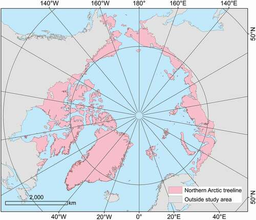
Our study area covers all of earth’s northern lands for more than 7 million km², including six regions: Alaska, Canada, Greenland, Iceland, Norway and Russia. The spatial extent of our study area is shown in the Figure 1. The study area includes the entire circumpolar area northward the Arctic treeline. Arctic treeline is the northernmost limit of Arctic Bioclimate Zone where trees can grow and the boundary between tundra and boreal forest, with length of 13,000 kilometers. Beyond the treeline that it is too cold all year round to sustain trees (Smol, Pienitz, & Douglas, 2004).

Figure 1. Spatial extent of the study area.

2.2. Multi-source remote sensing datasets

• Sentinel-1 SAR GRD Data

The Sentinel-1 constellation (S1-A and S1-B) provides C-band SAR imagery at a variety of polarizations and resolutions, and offers a 6-day revisit time for A/B constellation. (Berger, Moreno, Johannessen, Levelt, & Hanssen, 2012). Among various Sentinel-1 products, we used the Ground Range Detected (GRD) data, which are acquired in interferometric wide swath with dual polarization (VV and VH) and have a 10-m pixel spacing resolution. The Sentinel-1 Level-1 GRD products make available and have been implemented on the GEE, which are suitable for the most of the land application (Balzter, Cole, Thiel, & Schmullius, 2015; Hu et al., 2021; Lehner, Naeimi, & Steinnocher, 2017). Each Sentinel-1 image on the GEE was preprocessed with the Sentinel-1 toolbox, including thermal noise removal, radiometric calibration ant terrain correction (https://developers.google.com/earth-engine/sentinel1). By calculating the mean at pixel level derived individually for ascending and descending orbits and VV and VH polarization respectively, we generated three seasonal time-series metrics (spring, summer, and winter) of backscatter using all GRD images available in 2020 (Todar, Attarchi, & Osati, 2021).

• Sentinel-2 MSI

We also collected all the Sentinel-2 MSI Level-2A surface reflectance (SR) data available in 2020, and filtered them with a criterion of cloud cover less than 10%. Cloud and cloud shadows were mask according to the cloud mask band (QA60). Based on the Sentinel-2 composition, we generated all the corresponding median bands reflectance which are resampled to 10 m before (Blue, Green, Red, Red Edge1, Red Edge 2, Red Edge 3, Red Edge 4, NIR, SWIR1 and SWIR2). Then, the 10^th and 90^th percentile of NDVI (Normalized Difference Vegetation Index), NDBI (Normalized Built-up Index) and MNDWI (Modified Normalized Water Index) were calculated given that they have been demonstrated to help identify the impervious areas (Lin, Zhang, Lin, Gamba, & Liu, 2020; Liu et al., 2018; Xu, 2008, 2010). Meanwhile, we adopted a new variable (MNDWI minus NDBI) to highlight the difference between seasonal dry river bed and impervious areas.

Six textural metrics were generated according to a previous study on urban classification (Attarchi, 2020; Haralick, Shanmugam, & Dinstein, 1973). We calculated the contrast, variance, sum variance, dissimilarity, inertia and cluster prominence based on the Gray Level Co-occurrence Matrix (GLCM) for the Sentinel-2 NIR band with a $7\times 7$ moving window kernels (Zhang et al., 2020).

• ArcticDEM

ArcticDEM was released in 2016 with a high spatial resolution of 2 m, which derived from the optical stereo imagery, and the DEMs were compiled to reduce void areas and edge-matching artifacts. Three metrics, elevation, slope and aspect, were generated from the ArcticDEM (Zhang et al., 2020).

• OpenStreetMap

OpenStreetMap (OSM) (www.openstreetmap.org) is a free map of the world created by an ever-growing community of volunteered mappers and it provides the main infrastructure information (Hjort et al., 2018). Considering its positional accuracy which had been assessed in the past (Fan, Zipf, Fu, & Neis, 2014; Girres & Touya, 2010; Haklay, Basiouka, Antoniou, & Ather, 2010), it is thought to be a first-order positional accuracy geodata product for all data used and free-of-charged, especially in referenced geodata lacking areas, and OSM has been used for training data in pervious impervious mapping studies (Lin et al., 2020; Parekh et al., 2021). Although accuracy assessment of OSM is still lack in the Arctic regions, it is a simplification for large-scale analysis, which we assumed that our RF classified model can tolerate the noise caused by the OSM data. The geo-tapped information, i.e. OSM-Buildings, OSM-land use, OSM-Railways and OSM-Roads, covered the study area was used to produce a binary impervious areas map. Furthermore, we reclassified the OSM-land use into some sub-categories, including industrial, resident, public, military, commercial, transport, roads to indicate the impact of varies human activities.

2.3. Global impervious areas products

Considering almost no thematic product about circumpolar Arctic artificial impervious areas, two global land cover products in 2020 (GlobeLand30 and Esri-GLC) and a global thematic impervious areas product in 2015, MSMT-IS30, were selected to compare with our new CAMI product.

• GlobeLand30

GlobeLand30 is a 30 m global land-cover dataset produced using the Pixel-Object-Knowledge-based (POK-based) method with a reported overall accuracy of 85.72% (Chen et al., 2015). Recently it was updated to the 2020 version. This new version GlobeLand30 consists of 10 first-class land cover types, and we extracted the impervious areas from 10 types.

• Esri-GLC

Esri Land Cover is a latest 10-m global land-cover dataset, and it was produced using a deep learning AI classification model based on Microsoft Planetary Computer (Karra et al., 2021). It contains 10 land-cover classes and was reported with an overall accuracy of 85.96%. Similarly, we also extracted the impervious areas from that the original land cover map.

• MSMT-IS

MSMT-IS is a 30-m global impervious areas product produced by multi-source and multi-temporal random forest classification method based on GEE platform (Zhang et al., 2020). The overall accuracy of the map achieves 96.6%, and the impervious areas in our study area were extracted.

3. Methods

Figure 2 presents the workflow of our CAMI mapping method on the GEE platform. Particularly, the framework includes three sequentially integrated steps. In the first part, we developed a training and validation samples collection strategy based on prior knowledge derived from Globeland30 and OSM data. In the second part, we implemented a region-specified Random Forest classification via the 33 features (Table 1) derived from Sentinel-1/2 imagery, Arctic DEM and OSM data. Then, Arctic thematic impervious areas map was generated after filtering the isolated bare lands pixels. Finally, we evaluated our CAMI map with validation samples and three existing impervious areas products. We also analyzed current land use pattern within our CAMI map.

Figure 2. Workflow of our proposed approach for the CAMI mapping.

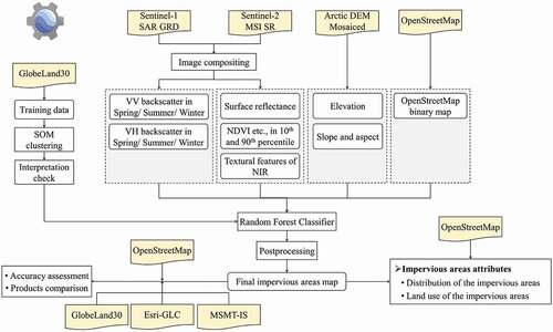
Table 1. All of 33 features used in the RF model.

Data	Features	Variable Names
Sentinel-1 SAR	Mean of VV in spring, summer and winter	VV_Spring, VV_Summer, VV_Winter
	Mean of VH in spring, summer and winter	VH_Spring, VH_Summer, VH_Winter
Sentinel-2 MSI	Reflectance: blue, green, red, red edge1,2,3,4, NIR and SWIR1,2	B2, B3, B4, B5, B6, B7, B8, B8A, B11, B12
	Normalized indices: 10^th percentile of NDVI, MNDWI and NDBI	NDVI10, MNDWI10, NDBI10
	Normalized indices: 90^th percentile of NDVI, MNDWI and NDBI	NDVI90, MNDWI90, NDBI90
	Normalized indices: mean MNDWI $-$ mean NDBI	WI_BI_diff
	Textural variables: contrast, variance, sum variance, dissimilarity, inertia and cluster prominence of the NIR	B8_Contrast, B8_Variance, B8_Sum_Variance, B8_Dissimilarity, B8_Inertia, B8_Cluster_Prominence
DEM	Elevation, slope and aspect	Elevation, Slope, Aspect
Auxiliary data	OpenStreetMap	OSM

3.1. Training and validation samples collection

A three-step training samples collection method was developed to refine training samples from GlobeLand30. Firstly, we randomly generated the geometric location of training samples for 10 land cover types using the stratified random sampling method based on their proportion in GlobeLand30. For each type, the number of the original training samples varies from 1000 to 5000. Among them, samples originally labeled as impervious in GlobaLand30 were assigned as impervious class, while other samples were assigned as non-impervious class. Then, in order to filter the outliers induced by mis-classified or omitted-classified in GlobaLand30, these training samples were clustered using the Self-organizing Map (SOM) clustering algorithm. Finally, the samples in the new clusters were visually check and interpreted via the available high-resolution remote sensing imagery in Google Earth. A total of 97656 training samples were collected, including 83158 non-impervious samples and 14498 impervious samples.

Compared with urban areas, the impervious areas in the Arctic are relatively small and scattered. The traditional random sampling method in such a situation may cause an overestimation of user accuracy. Good practices indicate that setting up some validation samples in buffer zones around the real impervious areas within an appropriate distance can reduce this overestimation (Liu et al., 2019). Here, we used OSM-Land use sub-data-set as the real impervious areas data and randomly generated a part of validation samples within the OSM patches. In addition, we selected some probability samples in the buffer zones. The detailed steps are illustrated in the following Figure 3.

Figure 3. Validation sampling strategy.

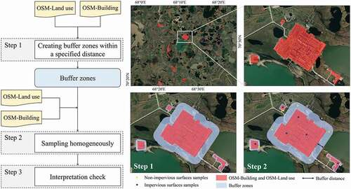
For the first step, we directly created buffer zones within a specified distance around each OSM-Land use patch. The specified distances were determined so that the buffer zone has approximately the same area as the OSM-Land use patch. Here, we assumed all OSM-Land use patches as regular rectangle, the relationship between the buffer distance and OSM-Land use patch can be described as the following formula:

(1) $bufferdistance=\frac{-P+\sqrt{P^2+16A}}{8}$(1)

Where P and A are the perimeter and area of the OSM-Land use patch respectively. The area radio of the buffer zone and the OSM-Land use patch achieves 0.96 to 0.98 statistically. Then, we randomly generated validation samples from the OSM-Land use area and the buffer area respectively. The size of the impervious or non-impervious collection validation samples was the same. Lastly, all the samples were checked by interpretation via available high-resolution remote sensing imagery in Google Earth.

Using the new sampling strategy, a total of 2693 validation samples were generated, including 1431 non-impervious samples and 1262 impervious samples.

3.2. Impervious areas extraction with random forest model

Random Forest (RF), which has obvious advantages in feature selection and classification, is considered to present a high level of robustness with respect to high-dimension multicollinearity data and noise (Oshiro, Perez, & Baranauskas, 2012). RF was chosen here for its relatively low computational cost but high accuracy performance while handling a large number of features with large training sample sizes among several classification algorithms and has been used in previous impervious mapping studies (Huang et al., 2020; Li, Gong, & Liang, 2015; Li, Wang, Wang, Hu, & Gong, 2014; Liu et al., 2019). There were 33 features derived from multi-source data, including 15 spectral features and 6 textural features from the Sentinel-2 imagery, six seasonal time-series metrics from SAR imagery, 3 topographical features and OSM binary feature, were feed into the RF model. Through a preliminary test, the optimal value for the number of trees was 500, and the number of variables to split on each node was set to 10. We divided the training sample pixels into two parts, 80% of them were used for training, and the remaining 20% were employed for testing the RF classification model. Meanwhile, to speed up the implement efficiency, we built RF classifiers for six regions: Alaska, Canada, Greenland, Russia, except for Iceland and Norway, which were combined due to these two regions have tiny shares of training samples.

3.3. Accuracy assessment

To assess the performance CAMI product, we used the validation samples collected by our proposed sampling strategy to calculate the accuracy. Four common accuracy metrics, including the overall accuracy (O.A.), the producer’s accuracy (P.A.), user’s accuracy (U.A.) as well as kappa coefficient were used to quantitatively assess the classification accuracy. Meanwhile, we also calculated the same accuracy indexes for other three existing impervious areas products (GlobeLand30, Esri-GLC and MSMT-IS) as references. Except for the quantitative estimation, we also analyze their detailed spatial patterns in small scale, in hope to better understand the pros and cons of our mapped results.

4. Results

4.1. Assessment of the impervious areas extent

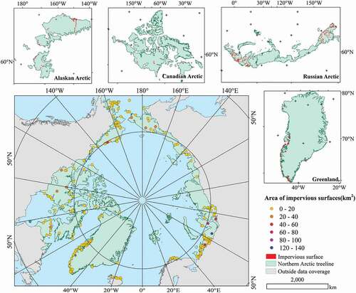
As shown in Figure 4, the majority of the impervious areas in the Arctic are fragmented and tiny in size, ranging from 42 $m^2$ to 132.29 $k{m}^2$. 94.50% impervious areas in the Arctic are under 20 $k{m}^2$, while 9.17% of them exceeds 80 $k{m}^2$, that mostly appear in Alaska and Western Russian Arctic. To better show the distribution pattern of the impervious areas in different regions, four representative regions are selected for comparison, including Alaska, Canadian Arctic, Russian Arctic and Greenland. Russian Arctic has the greatest number of impervious clusters, most of which distribute in the eastern and western inner land. However, in other three regions, impervious areas only locate along the coastline.

Figure 4. Distribution of impervious areas in the northern Arctic treeline. Every point in the map refers to the location of the centroid of the impervious areas and its color refers to the area. The highlighted sites in the map are located in Alaska, Canada, Russia and Greenland.

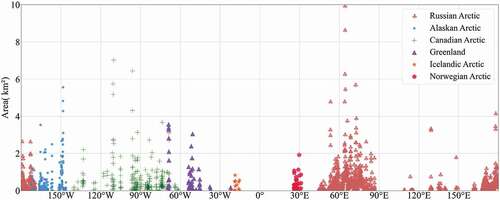
The meridional and zonal total impervious surface area for each $0.05°$ longitude and latitude interval are shown in Figures 5 and 6. We found in the zonal statistics (Figure 5) result that 90% of the impervious areas distribute between $60°$ and $80°$ and the impervious areas with medium to large size mostly locate between $64°$ and $72°$. The meridional results (Figure 6) illustrate that there are three peak intervals: $150°$ to $160°$ (Alaskan Arctic), $90°$ to $120°$ (Canadian Arctic) and $80°$ to $0.05°$ (Western Russian Arctic).

Figure 5. Distribution of zonal impervious areas calculated by $0.05°$ interval.

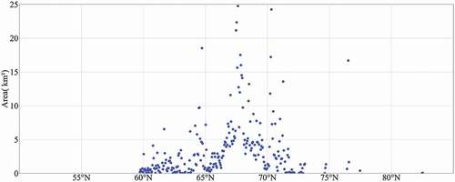
Figure 6. Distribution of meridional impervious areas calculated by $k{m}^2$ interval.

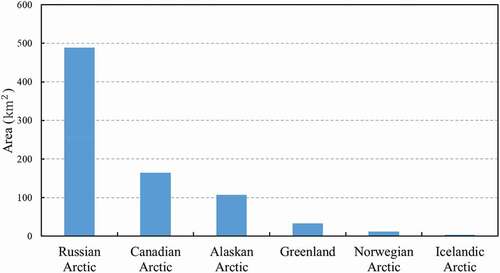
The total impervious surfaces area in the Arctic reaches 807.80 $k{m}^2$, and Figure 7 presents the impervious surfaces area at national scale. Russian Arctic has the biggest impervious surfaces area, accounting for more than 60.5%, followed by the 20.3% of the Canadian Arctic and 13.2% of the Alaskan Arctic. The three other countries account for less than 5% of the total area.

Figure 7. Impervious surfaces area in different regions.

4.2. Accuracy assessment using validation samples

Our result achieves the highest overall accuracy of 86.36% and kappa coefficient of 70.73% as listed in Table 2. The overall accuracy and kappa coefficient are also calculated for the three existing impervious areas products, which are 83.76% and 64.82% for GlobeLand30, 77.50% and 49.20% for Esri-GLC, 76.69% and 52.89% for MSMT-IS30, respectively. Both overall accuracy and the kappa coefficient are lower than that of Esri-GLC and MSMT-IS. As we observed, the validation samples they used are absent or distributed sparsely in the Arctic regions. In other words, impervious areas in the Arctic have not been specifically validated. The validation samples in this study are distributed within the Arctic, and we focused on the Arctic regions for validation and comparison.

Table 2. Accuracy of the four impervious areas maps using validation samples.

		Alaskan Arctic	Canadian Arctic	Greenland	Icelandic Arctic	Norwegian Arctic	Russian Arctic	Overall
This study	O.A.	85.71%	92.59%	88.19%	85.32%	78.14%	85.09%	86.36%
	Kappa	69.94%	82.64%	73.98%	69.57%	49.43%	69.29%	70.73%
	P.I.	70.65%	82.11%	82.14%	74.74%	52.42%	74.34%	73.91%
	U.I.	94.89%	94.71%	83.94%%	89.87%	82.28%	90.52%	90.32%
	P.N.	97.12%	97.74%	91.47%	93.50%	93.33%	93.74%	94.70%
	U.N.	81.38%	91.74%	90.42%	82.73%	76.86%	81.97%	84.42%
GlobeLand30	O.A.	88.52%	90.77%	74.62%	74.31%	76.65%	84.86%	83.76%
	Kappa	76.56%	77.81%	33.88%	45.81%	44.88%	68.95%	64.82%
	P.I.	85.87%	74.31%	29.29%	54.74%	45.97%	76.46%	68.02%
	U.I.	87.29%	97.01%	95.35%	80.00%	83.82%	87.98%	88.87%
	P.N.	90.53%	98.87%	99.22%	89.43%	94.76%	91.61%	94.29%
	U.N.	89.43%	88.66%	72.11%	71.90%	74.81%	82.88%	81.49%
Esri-GLC	O.A.	73.07%	78.21%	77.39%	78.90%	70.94%	77.84%	77.50%
	Kappa	41.01%	41.82%	44.01%	54.70%	43.53%	53.41%	49.20%
	P.I.	40.76%	37.16%	42.86%	52.63%	46.77%	56.11%	48.34%
	U.I.	92.59%	92.05%	85.71%	98.04%	96.67%	90.57%	91.57%
	P.N.	97.53%	98.42%	96.12%	99.19%	98.18%	95.31%	97.02%
	U.N.	68.50%	76.09%	75.61%	73.05%	62.07%	72.98%	73.71%
MSMT-IS30	O.A.	81.03%	80.94%	/	/	73.95%	73.74%	76.69%
	Kappa	59.37%	50.28%	/	/	37.73%	44.90%	52.89%
	P.I.	58.15%	44.95%	/	/	39.52%	90.75%	72.58%
	U.I.	96.40%	94.23%	/	/	80.33%	70.42%	75.47%
	P.N.	98.35%	98.65%	/	/	94.29%	52.57%	80.15%
	U.N.	75.63%	78.46%	/	/	72.53%	82.04%	77.65%

P.I., producer’s accuracy of impervious areas, U.I., user’s accuracy of impervious areas, P.N., producer’s accuracy of non-impervious areas, U.N., user’s accuracy of non-impervious areas. MSMT-IS30 lacked of impervious areas result in Greenland and Iceland.

Our result outperforms other existing land cover products from the perspective of the producer’s accuracy and user’s accuracy. Only MSMT-IS30 shows similar performance as CAMI according to the producer’s accuracy. However, Esri-GLC presents a negligible higher user’s accuracy than that of our products (91.57% VS 90.32%), its low producer’s accuracy (48.34%) implies that a huge omission of the impervious areas.

Specifically, the producer’s accuracy of impervious areas and kappa coefficient varies in different regions. Canadian Arctic, Greenland, Icelandic Arctic and Norwegian Arctic in our result have the highest producer’s accuracy of impervious areas. GlobeLand30 has the best performance in Alaska and MSMT-IS30 performs well in Russia. The user’s accuracy from our products exceeds 80% in all the regions.

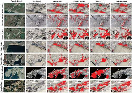
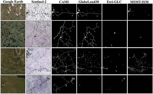
To further compare the performance of these four products, seven representative plots were selected for comparison as shown in Figure 8. Our result performs analogously with GlobeLand30, but is more sufficient in detailed impervious information, especially for roads. Roads are continuous and connected in CAMI, while they are broken and scarce in other three products. Esri-GLC has the least cover of linear imperviousness among the four products. Moreover, Esri-GLC has been overestimated because that the urban green land and bare lands are also identified as impervious areas. MSMT-IS30 missed impervious areas data in Greenland and Iceland, although it performs well than Esri-GLC in other regions.

Figure 8. Comparison between the method result (the third column) and the three other impervious products (the 4th to 6th columns corresponded to the GlobeLand30, Esri-GLC and MSMT_IS) for six plots. The second column is the corresponding RGB-composite Sentinel-2 images in 2020.

4.3. Land use of impervious areas in Arctic

Land use changes are caused by human-induced activities and further affect the environment and climate changes in entire Arctic. To further explore their land use status, we presented the land use pattern by calculating their area ratio based on OSM. The results are shown in Figures 9 and 10.

Figure 9 shows that Arctic has the most land uses in road, industrial, resident types, except for the unclassified type. Particularly, Russian Arctic, Norwegian Arctic, Canadian Arctic and Alaskan Arctic have the high cover of roads, accounting for 62.65%, 43.42%, 48.48% and 41.84% respectively. Iceland has more resident land as well as Greenland.

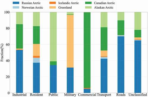
As shown in Figure 10, Russian Arctic is the main contributor of industrial land, roads, resident and transport land. More than 50% of the public land portion in the Arctic is dominated by Alaska. Military and commercial land are mostly located in Greenland and Canadian Arctic.

Figure 9. Area proportion of impervious land-use in Russia, Norway, Iceland, Greenland, Canada and Alaska. The impervious areas for industrial use contains industrial and mining land, for public use contains parks, cemetery and parking lots, for transport use contains airport and apron. Unclassified class refers to the impervious areas with unknown land-use identification in OSM dataset.

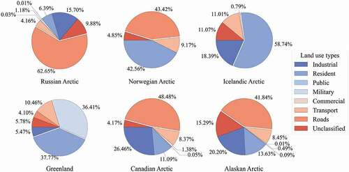
Figure 10. Stacked bar of 8 impervious land-use class in Arctic and its fraction of every country (region).

5. Discussion

5.1. The advantages of multi-source features

It is very hard to accurately map impervious areas using only optical remote sensing imagery due to the spectral heterogeneity. The incorporation of multi-source data features added more useful information except for spectral dimension. In this study, we found multi-source date made contributions to high accuracy of CAMI. OSM, DEM and optical imagery were the three high-contributed data sources. Our research further explored their relative contribution within all 33 features for impervious areas mapping among six regions, which is illustrated in Figure 11.

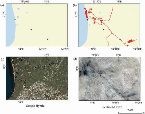
The OSM metrics obviously outperformed in all of the features. One reason is that OSM provides the prior knowledge that might reduce the confusion error caused by bare soils to some extent. On the other hand, OSM contains detailed subcategory of impervious areas, which supplemented abundant impervious information, especially when the impervious areas are not easy to be detected. Although, not all the study area covers the OSM data, our robust RF training model by integrating the multi-source datasets, such as, optical images, SAR data and topographic data, could transfer the prior knowledge to other regions without OSM data via the decision tree model. Figure 12(b) shows the detailed spatial pattern of our impervious areas and it indicates that our method could dig all the impervious areas in the region with incomplete OSM.

Generally, the DEM-related features contributed the second highest, although their importance varies among different regions. Spectral-related features and four indexes (NDVI, NDBI, MNDWI, and the difference between MNDWI and NDBI) were ranked third. In addition, the importance of SAR features was inferior to optical features.

Figure 11. The importance of the input features derived from the random forest model using the training samples in six regions. Mean decrease in accuracy was used to assess the importance of the input features, which refers how much the model accuracy decreases if that variable was dropped. The bar with different colors refers the mean importance of the different data sources.

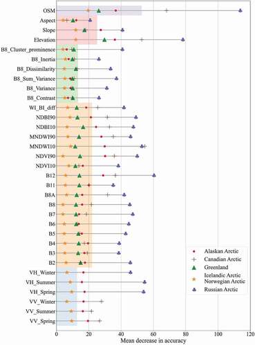
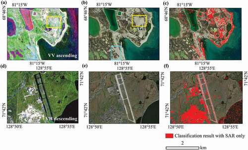
Figure 12. Example of classification results of human-impacted areas in comparison to OpenStreetMap and the Google Earth online hybrid map in Yamal, Russia: (a) OpenStreetMap (blue-waterbodies, grey-roads); (b) classification results based on this study; (c) Google Earth online hybrid map; (d) Sentinel-2 red-green-blue (band 4-3-2) composition in 2020. Projection WGS_1984_EPSG_Russia_Polar_Stereographic.

We noticed that the features from the SAR data does not show a high importance compared to the traditional impervious areas mapping in urban areas (Attarchi, 2020; Delgado Blasco, Fitrzyk, Patruno, Ruiz-Armenteros, & Marconcini, 2020). This can be partly explained by the limited coverage of SAR in the entire Arctic, especially for high latitudes. Furthermore, in urban areas, the diversity of the urban building, such as the linear arrangement of houses, the dimensions of the streets, the type of buildings (i.e. numerous planes of the roof), resulting in the higher backscattering than other land cover types, especially the higher double bounce backscattering induced by the dihedrals. While, in our study area, the impervious areas shows same roughness as other land cover types, such as bare lands near the seasonal dry river bed (Figure 13(a–c)). Meanwhile, the smooth concrete ground and the airport, a common impervious areas type in Arctic, also show similar low backscattering when compared with waterbodies (Figure 13(d–f)). Relatively low roughness of the impervious areas in the Arctic might cause overestimation of the impervious areas due to the commission of bare lands, while, the omission of the smooth impervious areas might bring a underestimation of it.

Figure 13. Examples of human-impacted areas in comparison to SAR images, Google Earth and classification result with SAR derived features only in Arctic: the first column refers the Sentinel-1 spring-summer-winter composition in 2020, the second column refers Google Earth online hybrid map and the third column refers the classification result based on the SAR derived features. The highlighted boxes in yellow indicate the true impervious areas and cyan boxes indicate the bare lands.

5.2. Uncertainties and implications of our impervious surface map

Although the proposed method has been demonstrated to have the ability to map the impervious areas in Arctic with a high overall accuracy of 86.36%, there are still some uncertainties. First, Due to the difficulty of collecting training samples in field, our training samples is collected from GlobeLand30. Some scattered and low-density impervious samples might be omitted and this could cause further omission of the scattered and small impervious surfaces, such as the fragmented villages, pipelines and informal trails. Second, such comparably small settlements and linear features cannot be completely captured due to the medium spatial resolution imagery. Figure 14 shows that CAMI has advantages on detailed roads compared to the other products. Moreover, it is still rooms for CAMI to connect the broken roads or pipelines. Third, the existing impervious areas products generally lack of subcategories of impervious areas classes. Although we subdivided them into a given land use attribute based on OSM data, identifying their land use types based on the multi-sources remotely sensed imageries and point of interest data is worthy of more attention.

Despite this limitation, our CAMI product is still a good supplement to previous coarser spatial resolution and incomplete data in the Arctic. We believe that our finer resolution CAMI product can support some significate research, such as the vulnerability of the infrastructure, the urbanization and vegetation changes due to the human activities in this region (Hjort et al., 2018; Miles & Esau, 2017; Raynolds et al., 2014).

Figure 14. Roads comparison between CAMI and the three impervious surfaces products (the 4^th to 6^th columns corresponded to the GlobeLand30, Esri-GLC and MSMT_IS30) for four plots. The second column is the corresponding RGB-composite Sentinel-2 images in 2020.

6. Conclusions

It is a challenging task to precisely map the impervious areas in the Arctic due to the small proportion, diversity of its composition, and uneven distribution of area. In this study, we developed a 10-m resolution CAMI map with the use of the Sentinel-1 and −2 time series data, OpenStreetMap and ArcticDEM via Google Earth Engine platform. Comparing with the existing global land cover products in the Arctic, the CAMI product has a high overall accuracy of 86.36% across the Arctic and this reveals the feasibility of our approach. Furthermore, our map estimates the total impervious surfaces area in the Arctic achieves 807.80 $k{m}^2$, and it has the most land uses of roads, industrial and resident lands. Our CAMI map can serve as a base data for studying Arctic infrastructure vulnerability and ecological sustainable development. Higher spatial resolution data source, such as GF series imagery, can be then considered for improving impervious areas mapping in the Arctic. And Further work should focus on monitoring impervious areas dynamic and analyzing its driving factors via the long time-series satellite images.

Disclosure statement

No potential conflict of interest was reported by the author(s).

Data availability statement

The CAMI map will be openly accessed at http://www.doi.org/10.11922/sciencedb.01435

Additional information

Funding

This research was supported by the National Key R&D Program of China [2018YFC1407103 and 2017YFA0604401] and Annual Report (2022) on Remote Sensing Monitoring of Global Ecosystems and Environment [TC210E01B].

Notes on contributors

Xiaoqing Xu

Xiaoqing Xu received the B.S. degree from South China Agricultural University. She is currently working toward the M.S. degree in School of Geospatial Engineering and Science, Sun Yat-Sen University. Her research interests include land cover mapping and application in polar regions.

Chong Liu

Chong Liu received his Ph.D. degree in remote sensing science from the State Key Laboratory of Information Engineering in Surveying, Mapping and Remote Sensing (LIESMARS), Wuhan University in 2015. He is now a research associate Professor of School of Geospatial Engineering and Science, Sun Yat-Sen University. Dr. Liu’s research interests focus on environmental impacts of land use/cover and climate change with remote sensing techniques and methods.

Huabing Huang

Huabing Huang Huabing Huang received his Ph.D. degree from the Institute of Remote Sensing and Digital Earth, Chinese Academy of Sciences. He is currently a professor in School of Geospatial Engineering and Science, Sun Yat-Sen University. His major research interests focus on dynamics land cover monitoring, vegetation height/biomass mapping with spaceborne Lidar.

References

- AMAP. (2017). Snow, Water, Ice and Permafrost in the Arctic (SWIPA) 2017.
- Arnold, C. L., & Gibbons, C. J. (1996). Impervious surface coverage: The emergence of a key environmental indicator. Journal of the American Planning Association, 62(2), 243–258.
- Attarchi, S. (2020). Extracting impervious surfaces from full polarimetric SAR images in different urban areas. International Journal of Remote Sensing, 41(12), 4644–4663.
- Balzter, H., Cole, B., Thiel, C., & Schmullius, C. (2015). Mapping CORINE land cover from sentinel-1A SAR and SRTM digital elevation model data using random forests. Remote Sensing, 7(11), 14876–14898.
- Bartsch, A., Pointner, G., Ingeman-Nielsen, T., & Lu, W. (2020). Towards circumpolar mapping of arctic settlements and infrastructure based on sentinel-1 and sentinel-2. Remote Sensing, 12(15), 2368.
- Bartsch, A., Pointner, G., Nitze, I., Efimova, A., Jakober, D., Ley, S., … Schweitzer, P. (2021). Expanding infrastructure and growing anthropogenic impacts along Arctic coasts. Environmental Research Letters, 16(11), 115013.
- Beamish, A., Raynolds, M. K., Epstein, H., Frost, G. V., Macander, M. J., Bergstedt, H., … Wagner, J. (2020). Recent trends and remaining challenges for optical remote sensing of Arctic tundra vegetation: A review and outlook. Remote Sensing of Environment, 246, 111872.
- Berger, M., Moreno, J., Johannessen, J. A., Levelt, P. F., & Hanssen, R. F. (2012). ESA’s sentinel missions in support of Earth system science. Remote Sensing of Environment, 120, 84–90.
- Brown de Colstoun, E. C., Huang, C., Wang, P., Tilton, J. C., Tan, B., Phillips, J., … Wolfe, R. E. (2017). Global Man-made Impervious Surface (GMIS) dataset from landsat. Palisades, NY: NASA Socioeconomic Data and Applications Center (SEDAC).
- Brun, S. E., & Band, L. E. (2000). Simulating runoff behavior in an urbanizing watershed. Computers, Environment and Urban Systems, 24(1), 5–22.
- Chen, J., Chen, J., Liao, A., Cao, X., Chen, L., Chen, X., … Mills, J. (2015). Global land cover mapping at 30m resolution: A POK-based operational approach. ISPRS Journal of Photogrammetry and Remote Sensing, 103, 7–27.
- Delgado Blasco, J. M., Fitrzyk, M., Patruno, J., Ruiz-Armenteros, A. M., & Marconcini, M. (2020). Effects on the double bounce detection in urban areas based on SAR polarimetric characteristics. Remote Sensing, 12, 1187.
- Fan, H. C., Zipf, A., Fu, Q., & Neis, P. (2014). Quality assessment for building footprints data on OpenStreetMap. International Journal Of Geographical Information Science, 28(4), 700–719.
- Feng, Y., Ziegler, A. D., Elsen, P. R., Liu, Y., He, X. Y., Spracklen, D. V., … Zeng, Z. Z. (2021). Upward expansion and acceleration of forest clearance in the mountains of Southeast Asia. Nature Sustainability, 4(10), 892–899.
- Girres, J. F., & Touya, G. (2010). Quality assessment of the French OpenStreetMap dataset. Transactions in GIS, 14, 435–459.
- Gong, P., Li, X., Wang, J., Bai, Y., Chen, B., Hu, T., … Zhou, Y. (2020). Annual maps of global artificial impervious area (GAIA) between 1985 and 2018. Remote Sensing of Environment, 236, 111510.
- Gong, P., Liu, H., Zhang, M., Li, C., Wang, J., Huang, H., … Song, L. (2019). Stable classification with limited sample: Transferring a 30-m resolution sample set collected in 2015 to mapping 10-m resolution global land cover in 2017. Science Bulletin, 64(6), 370–373.
- Gong, P., Wang, J., Yu, L., Zhao, Y., Zhao, Y., Liang, L., … Chen, J. (2013). Finer resolution observation and monitoring of global land cover: First mapping results with Landsat TM and ETM+ data. International Journal of Remote Sensing, 34(7), 48.
- Gorelick, N., Hancher, M., Dixon, M., Ilyushchenko, S., Thau, D., & Moore, R. (2017). Google earth engine: Planetary-scale geospatial analysis for everyone. Remote Sensing of Environment, 202, 18–27.
- Grimm, N. B., Faeth, S. H., Golubiewski, N. E., Redman, C. L., Wu, J., Bai, X., & Briggs, J. M. (2008). Global change and the ecology of cities. Science (New York, N.Y.), 319(5864), 756–760.
- Haklay, M., Basiouka, S., Antoniou, V., & Ather, A. (2010). How many volunteers does it take to map an area well? The validity of Linus’ law to volunteered geographic information. The Cartographic Journal, 47(4), 315–322.
- Haralick, R. M., Shanmugam, K., & Dinstein, I. (1973). Textural features for image classification. IEEE Transactions on Systems, Man, and Cybernetics, SMC-3(6), 610–621.
- Hjort, J., Karjalainen, O., Aalto, J., Westermann, S., Romanovsky, V. E., Nelson, F. E., … Luoto, M. (2018). Degrading permafrost puts Arctic infrastructure at risk by mid-century. Nature Communications, 9(1), 5147.
- Homer, C. G., Huang, C., Yang, L., Wylie, B. K., & Coan, M. (2004). Development of a 2001 national land cover database for the United States. Photogrammetric Engineering And Remote Sensing, 70(7), 829–840.
- Hu, B., Xu, Y. Y., Huang, X., Cheng, Q. M., Ding, Q., Bai, L. Z., & Li, Y. (2021). Improving urban land cover classification with combined use of sentinel-2 and sentinel-1 imagery. ISPRS International Journal Of Geo-Information, 10(8), 533.
- Huang, H., Wang, J., Liu, C., Liang, L., Li, C., & Gong, P. (2020). The migration of training samples towards dynamic global land cover mapping. ISPRS Journal of Photogrammetry and Remote Sensing, 161, 27–36.
- Karra, K., Kontgis, C., Statman-Weil, Z., Mazzariello, J. C., Mathis, M., & Brumby, S. P. (2021). Global land use/land cover with sentinel 2 and deep learning. 2021 IEEE International Geoscience and Remote Sensing Symposium IGARSS, Brussels, Belgium (pp. 4704–4707).
- Lehner, A., Naeimi, V., & Steinnocher, K. (2017). Sentinel-1 for urban areas comparison between automatically derived settlement layers from sentinel-1 data and copernicus high resolution information layers. GISTAM: Proceedings Of The 3rd International Conference On Geographical Information Systems Theory, Applications And Management, Porto, Portugal (pp. 43–49).
- Li, C. C., Wang, J., Wang, L., Hu, L. Y., & Gong, P. (2014). Comparison of classification algorithms and training sample sizes in urban land classification with landsat thematic mapper imagery. Remote Sensing, 6(2), 964–983.
- Li, X. C., Gong, P., & Liang, L. (2015). A 30-year (1984-2013) record of annual urban dynamics of Beijing City derived from Landsat data. Remote Sensing of Environment, 166, 78–90.
- Liang, L., Liu, Q., Liu, G., Li, H., & Huang, C. (2019). Accuracy evaluation and consistency analysis of four global land cover products in the arctic region. Remote Sensing, 11, 1396.
- Lin, Y., Zhang, H., Lin, H., Gamba, P. E., & Liu, X. (2020). Incorporating synthetic aperture radar and optical images to investigate the annual dynamics of anthropogenic impervious surface at large scale. Remote Sensing of Environment, 242, 111757.
- Liu, C., Huang, H., Hui, F., Zhang, Z., & Cheng, X. (2021). Fine-resolution mapping of pan-arctic lake ice-off phenology based on dense sentinel-2 time series data. Remote Sensing, 13, 2742.
- Liu, C., Zhang, Q., Luo, H., Qi, S., Tao, S., Xu, H., & Yao, Y. (2019). An efficient approach to capture continuous impervious surface dynamics using spatial-temporal rules and dense Landsat time series stacks. Remote Sensing of Environment, 229, 114–132.
- Liu, X., Hu, G., Chen, Y., Li, X., Xu, X., Li, S., & Pei, F. (2018). High-resolution multi-temporal mapping of global urban land using landsat images based on the Google earth engine platform. Remote Sensing of Environment, 209, 227–239.
- Miles, V., & Esau, I. (2017). Seasonal and spatial characteristics of urban heat islands (UHIs) in northern west Siberian Cities. Remote Sensing, 9, 989.
- Oshiro, T. M., Perez, P. S., & Baranauskas, J. A. (2012). How many trees in a random forest? In P. Perner (Ed.), Machine learning and data mining in pattern recognition (pp. 154–168). Berlin, Heidelberg: Springer Berlin Heidelberg.
- Parekh, J. R., Poortinga, A., Bhandari, B., Mayer, T., Saah, D., & Chishtie, F. (2021). Automatic detection of impervious surfaces from remotely sensed data using deep learning. Remote Sensing, 13(16), 3166.
- Raynolds, M. K., Walker, D. A., Ambrosius, K. J., Brown, J., Everett, K. R., Kanevskiy, M., … Webber, P. J. (2014). Cumulative geoecological effects of 62 years of infrastructure and climate change in ice-rich permafrost landscapes, Prudhoe Bay Oilfield, Alaska. Global Change Biology, 20(4), 1211–1224.
- Seto, K. C., Güneralp, B., & Hutyra, L. R. (2012). Global forecasts of urban expansion to 2030 and direct impacts on biodiversity and carbon pools. Proceedings of the National Academy of Sciences of the United States of America, 109(40), 16083–16088.
- Sexton, J. O., Song, X.-P., Huang, C., Channan, S., Baker, M. E., & Townshend, J. R. (2013). Urban growth of the Washington, D.C.–Baltimore, MD metropolitan region from 1984 to 2010 by annual, Landsat-based estimates of impervious cover. Remote Sensing of Environment, 129, 42–53.
- Shelestov, A., Lavreniuk, M., Vasiliev, V., Shumilo, L., Kolotii, A., Yailymov, B., … Yailymova, H. (2020). Cloud approach to automated crop classification using sentinel-1 imagery. IEEE Transactions on Big Data, 6(3), 572–582.
- Slonecker, E. T., Jennings, D. B., & Garofalo, D. (2001). Remote sensing of impervious surfaces: A review. Remote Sensing Reviews, 20(3), 227–255.
- Smol, J., Pienitz, R., & Douglas, M. (2004). Long-term environmental change in arctic and Antarctic lakes, Springer, Dordrecht.
- Song, X.-P., Hansen, M. C., Stehman, S. V., Potapov, P. V., Tyukavina, A., Vermote, E. F., & Townshend, J. R. (2018). Global land change from 1982 to 2016. Nature, 560(7720), 639–643.
- Todar, S. A. S., Attarchi, S., & Osati, K. (2021). Investigation the seasonality effect on impervious surface detection from sentinel-1 and sentinel-2 images using Google earth engine. Advances In Space Research, 68(3), 1356–1365.
- Wang, J. A., Sulla-Menashe, D., Woodcock, C. E., Sonnentag, O., Keeling, R. F., & Friedl, M. A. (2020). Extensive land cover change across Arctic-Boreal Northwestern North America from disturbance and climate forcing. Global Change Biology, 26(2), 807–822.
- Wang, P., Huang, C., Brown de Colstoun, E. C., Tilton, J. C., & Tan, B. (2017). Global Human Built-up And Settlement Extent (HBASE) dataset from landsat. Palisades, NY: NASA Socioeconomic Data and Applications Center (SEDAC).
- Weng, Q. (2012). Remote sensing of impervious surfaces in the urban areas: Requirements, methods, and trends. Remote Sensing of Environment, 117, 34–49.
- Wilder, B. (2012). Cloud architecture patterns: Using microsoft azure. O’Reilly Media, Inc.
- Wu, W., Guo, S., & Cheng, Q. (2020). Fusing optical and synthetic aperture radar images based on shearlet transform to improve urban impervious surface extraction. Journal of Applied Remote Sensing, 14(2), 024506.
- Xu, H. Q. (2010). Analysis of Impervious surface and its impact on urban heat environment using the normalized difference impervious surface index (NDISI). Photogrammetric Engineering And Remote Sensing, 76(5), 557–565.
- Xu, H. (2008). A new index for delineating built-up land features in satellite imagery. International Journal of Remote Sensing, 29(14), 4269–4276.
- Zhang, H., Lin, H., Li, Y., Zhang, Y., & Fang, C. (2016). Mapping urban impervious surface with dual-polarimetric SAR data: An improved method. Landscape and Urban Planning, 151, 55–63.
- Zhang, X., Liu, L., Wu, C., Chen, X., Gao, Y., Xie, S., & Zhang, B. (2020). Development of a global 30 m impervious surface map using multisource and multitemporal remote sensing datasets with the Google Earth Engine platform. Earth System Science Data, 12(3), 1625–1648.