Influence of changes in extreme daily rainfall distribution on the stability of residual soil slopes

ABSTRACT

Many landslides triggered by intense rainfall have occurred in mountainous areas in Thailand, causing major economic losses and infrastructure damage. Extreme daily rainfall is a significant trigger for hillslope instability. Increases in extreme daily rainfall intensity due to climate change may be one of the key factors responsible for the increased landslides. Thus, in this context, changes in the intensity of extreme daily rainfall in Chiang Mai Province in North Thailand and their effects on hillslope stability are analyzed. Extreme rainfall is modeled using a generalized extreme value distribution and estimated for various return periods. A numerical analysis of seepage and an infinite slope stability model are combined to understand the hillslope response under extreme rainfall conditions. The analysis period is divided into two periods of 34 years: 1952 to 1985 and 1986 to 2019. According to the analysis results, the distribution of extreme daily rainfall changes in terms of location. The average annual daily maximum rainfall increased by approximately 11.13%. The maximum decrease in the safety factor is approximately 4.5%; therefore, these changes in extreme daily rainfall should be considered in future landslide prevention policies.

KEYWORDS:

• Extreme rainfall
• generalized extreme value distribution
• slope stability
• landslide
• pore water pressure
• climate change
• residual soil

1. Introduction

Thailand is located in the tropical monsoon climate region and is affected by tropical cyclones. The southwest monsoons and tropical cyclones from the Pacific Ocean bring heavy rainfall in the rainy season, which is the main triggering factor for shallow landslides. Researchers have reported that extreme daily rainfall events induce shallow landslide cases. For example, the landslides and debris flows in southern Thailand in November 1988 were caused by extremely intense rainfall, with a peak daily intensity of rainfall greater than 400 mm on 21 November 1988 (Phien-wej, Nutalaya, Aung, & Zhibin, 1993). In August 2001, 24-hr rainfall of approximately 100 mm occurred in the Nam Ko village area in Phetchabun Province (Oh, Lee, Chotikasathien, Kim, & Kwon, 2009). As a result, a landslide and debris flow occurred, damaging housing and infrastructure and killing 136 people. Wang, Sassa, and Fukuoka (2003) reported that landslides and debris flows occurred in Hiroshima, Japan, due to heavy daily rainfall on June 29, 1999. The total 24-h rainfall on June 29, 1999, was 250 mm, and the peak hourly rainfall intensity reached 50 mm/h. In addition, in 2011, massive landslides occurred in the Krabi Province of Thailand. The landslides and debris flows at Khao Phnom, Krabi, occurred on March 28, 2011, when the 24-hr rainfall exceeded 200 mm (Chaithong, 2017). Thus, based on studies of these historical landslide cases, extreme daily rainfall events are one of the significant factors that can trigger landslides.

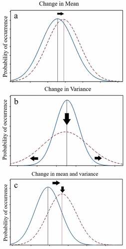
Recently, the sixth assessment report of the Intergovernmental Panel on Climate Change (IPCC, 2021) reported that there are increases in daily heavy rainfall amounts in the Southeast Asia region (IPCC, 2021). This indicates that Southeast Asian countries, including Thailand, may face more extreme daily rainfall events due to climate change. The issue of climate change is a global issue that every country attempts to fix. The United Nations assigned the climate change issue as goal number thirteen of sustainable development goals (SGDs), and this goal aims to take urgent action to combat climate change and its impact (United Nations, 2021). Thus, understanding changes in extreme daily rainfall are critical for disaster preparedness. There are broadly three simplified patterns of change in terms of changes in an extreme climate, including extreme daily rainfall (National Academies of Sciences, Engineering, and Medicine, 2016). The first pattern is changes in the mean or location, i.e. a simple shift in the probability distribution of the climate variable. The second, a change in the variance, means an increase in the variability of the probability distribution of the climate variable without necessarily being accompanied by a change in the position of the mean. The last aspect, i.e. changes in the mean, variance, and skewness, indicates that the shape of the probability distribution of the climate variable has changed; this is known as changed symmetry (Kodra & Ganguly, 2014). Figure 1 presents the patterns of changes in extreme climate. The generalized extreme value (GEV) distribution is widely used to determine the probability distribution function for the maximum or minimum values based on the block maxima method of extreme value theory. The generalized extreme value (GEV) distribution is often used to fit the rainfall distribution to consider extreme rainfall as a hydrological variable (Nadarajah, 2005; Park, Kang, Lee, & Kim, 2011; Yilmaz & Perera, 2014). For instance, Mishra and Singh (2010) used the generalized extreme value (GEV) distribution to study the changes in extreme precipitation in Texas. Moreover, Ragulina and Reitan (2017) used the generalized extreme value (GEV) distribution to assess the probability of extreme precipitation events in Europe and the United States.

Figure 1. Changes in the distribution of extreme climate variables: (a) change in mean, (b) change in variance, and (c) change in mean, variance and skewness.

The rainfall-induced shallow landslides has been studied extensively using two conceptual models based on the occurrence of slope failure (Collins & Znidarcic, 2004; Ning & Godt, 2013). In the case of the first mechanism, a significant positive pore water pressure is generated in the saturated slope due to the infiltration of rainfall (Eab, Likitlersuang, & Takahashi, 2015). The possible outcomes of this scenario include multidirectional seepage of groundwater into the soil slope and static liquefaction, resulting in rapid movement of the hillslope (Collins & Znidarcic, 2004). In the second mechanism, landslides occur due to a loss of unsaturated shear strength when the negative pore water pressure (i.e. soil matric suction) is reduced or dissipated due to rainfall infiltration (Collins & Znidarcic, 2004; Fredlund, 2006; Nguyen, Likitlersuang, & Jotisankasa, 2020). Given these mechanisms, changes in pore water pressure are generally recognized to be a significant cause of rainfall-induced shallow landslides, as rainfall infiltration is a primary cause of pore water pressure changes (Chatra, Dodagoudar, & Maji, 2019; Ning & Griffiths, 2004; Zhang, Zhang, Zhang, & Tang, 2011). Many researchers have used several methods to investigate the effect of rainfall on the stability of slopes, such as landslide flume experiments, numerical models or field investigations and monitoring to understand the mechanisms of rainfall-induced shallow landslides (Likitlersuang, Takahashi, & Eab, 2017; Nguyen, Likitlersuang, & Jotisankasa, 2019). Numerical models are successful methods of simulating pore water pressure profiles for slope stability models (Nguyen & Likitlersuang, 2019; Rahardjo, Li, Toll, & Leong, 2001; Tan, Ma, Chen, Ke, & Wang, 2009). Numerical models consider variations in the hydraulic conductivity of soil in the unsaturated soil zone, in which hydraulic conductivity is highly dependent on the water content of the soil (Cww & Shi, 1998). The infinite slope stability model is widely used to calculate the factor of safety in rainfall-induced shallow landslide models, such as the SINMAP, TRIGRS, SHALSTAB, and SLIP models (ZizioMichel, Kobiyama, & Goerl, 2014; Zizioli, Meisina, Valentino, & Montrasio, 2013). The failure mode in shallow landslides triggered by rainfall corresponds to the characteristics suggested by the infinite slope stability model. The depth-to-length ratio is small and the failure plane is parallel to the slope surface (Zhang et al., 2011).

Given this context, this study investigates the effects of changes in the extreme daily rainfall distribution on the stability of residual soil slopes in Chiang Mai Province in northern Thailand. To achieve this objective, the study uses the GEV distribution to capture the changing extreme daily rainfall distribution and generate intensity-frequency-duration (IDF) curves for extreme precipitation for two periods (1952 to 1985 and 1986 to 2019). The study also used a numerical model to simulate rainwater seepage and combined the results with the infinite slope stability model to calculate the safety factor to compare changes between the two studied periods.

2. Study area

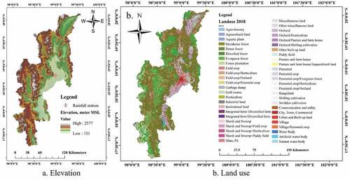
The area in this study was Chiang Mai Province, North Thailand. The rainfall and its intensity in Chiang Mai Province are influenced by the southwest monsoon and tropical cyclones originating in the South China Sea during the rainy season (May to October). The average annual rainfall is approximately 1,100 mm, and August and September are typically the wettest months in the province. Figure 2 presents (a) the elevation and (b) the land use of Chiang Mai Province. Topographically, the Chiang Mai province can be divided into two main regions: the plains and the mountainous region. Slope angles in the mountainous region of Chiang Mai Province broadly range in the interval of 17–40 degrees. In terms of land use, most of the mountainous region is either forested or used for agriculture. However, some residential areas are also present. The major residential and commercial areas are located in the plains region of the province.

Figure 2. (a) Elevation of Chiang Mai and (b) land use of Chiang Mai.

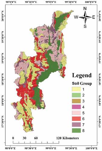
In terms of geological conditions, the Chiang Mai province comprises various rock types, including Triassic granite. In Thailand, nine soil groups relating to their landslide potential have been classified based on their parent rock, grain size distribution, density, and shear strength behavior (Phattanaprateep, 2016; Soralump & Thorwiwat, 2009). The residual soil formed by the weathering of carbonate rock (Group 7), Quaternary deposits (Group 8), and the sedimentary rock of the Khorat group (Group 9) exhibits low landslide probability in Thailand (Soralump, 2010). Figure 3 presents the soil groups related to landslide potential in Chiang Mai Province. In the case of Chiang Mai, eight of the residual soil groups in the plains region are based on Quaternary deposits.

Figure 3. Soil groups related to landslide potential in Chiang Mai Province.

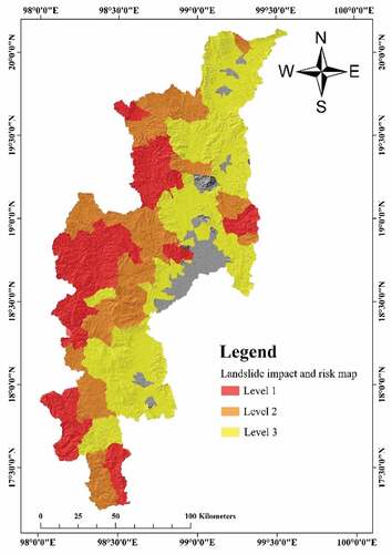
Regarding landslide susceptibility areas, the Department of Mineral Resources (DMR) of Thailand classifies landslide susceptibility into 3 levels. Level 1 is extremely high risk, and the direct impact is that the landslide occurred; the houses in villages are instantly destroyed by the failure of the slope and debris of the landslide. Level 2 is high risk and indirect impact, and Level 3 is medium risk and indirect impact. Figure 4 shows the landslide susceptibility map of Chiang Mai Province; the western part of the province is classified as Level 1, whereas the adjacent areas are classified as Level 2. The western part of the province forms a mountainous area with high slope gradients; therefore, the landslide risk in this area is high; however, the plains region of the province is considered to be a comparatively lower risk.

Figure 4. Landslide susceptibility map for Chiang Mai Province.

3. Method and data

3.1. Methods

The method used in this study can be divided into four steps. The first step is the analysis of extreme rainfall distributions using GEV and the generation of IDF curves. The second step is to estimate the soil-water characteristics curve (SWCC) and hydraulic conductivity function for seepage analysis. The third step is to perform a seepage analysis using a one-dimensional soil column model to simulate the hydrological responses. Finally, the last step of the analysis involves determining the stability of the slope using the infinite slope stability model and pore water pressure profile obtained from the seepage analysis of the various soil groups.

3.1.1. Extreme rainfall and generalized extreme value distribution

Normally, extreme climate events are defined based on their maximum values or when values exceed a particular percentile of a probability density function based on observations (Diaz & Murnane, 2008). As per extreme value theory, there are two main approaches the block maxima method and the excesses over threshold method. The block maxima method considers the data in blocks of equal length and performs calculations based on the maximum value in each block. The excesses over the threshold method restrict attention to data that exceeds some threshold. In this study, extreme rainfall is analyzed based on the block maxima method using the stationary GEV distribution. The cumulative distribution function (CDF) of the GEV distribution is given as follows:

(1) $F\left(x\right)=\left\{\begin{array}{c}exp\left[-{\left(1+\frac{\xi \left(x-\mu \right)}{\sigma }\right)}^{-\frac{1}{\xi }}\right];\xi \ne 0\\ exp\left[-exp\left(-\frac{x-\mu }{\sigma }\right)\right];\xi =0\end{array}\right\}$(1)

where $\mu$ is the location parameter, $\sigma$ is the scale parameter, and $\xi$ is the shape parameter. Moreover, when $\xi =0$, the GEV distribution is the Gumbel distribution; when $\xi >0$, the GEV distribution is the Fréchet distribution; and when $\xi <0$, the GEV distribution is the negative Weibull distribution. For IDF curves, the return period, T (in years), can be obtained from the following equation:

(2) $x_T=\mu -\frac{\sigma }{\xi }\left[1-{\left(-log\left(1-\frac{1}{P}\right)\right)}^{-\xi }\right]$(2)

when P = 1- (1/T)

The maximum likelihood estimation (MLE) method is used to fit the data. Let us assume that x₁, …, x_n denote the annual maximum daily rainfall for n years at the Chiang Mai monitoring station. Then, assuming that the rainfall data are independent, the likelihood is the product of the densities for observations x₁, …, x_n. Therefore, we have

(3) $L\left(\mu ,\sigma ,\xi \right)=\frac{1}{{\sigma }^n}\prod _{i=1}^n{\left(1+\xi \frac{x_i-\mu }{\sigma }\right)}^{-\left(1/\xi +1\right)}\times exp\left\{-\sum _{i=1}^n{\left(1+\xi \frac{x_i-\mu }{\sigma }\right)}^{-1/\xi }\right\}$(3)

The Anderson–Darling (AD) test and the p value were used to verify the goodness-of-fit of the distribution; the H0 hypothesis assumed that the data would follow the probability distribution at a significance level of 0.05. In addition, probability plots were also used to verify the goodness-of-fit of the distribution.

3.1.2. Soil-water characteristics curve and hydraulic conductivity function estimation

Considering unsaturated soil behavior, the SWCC and hydraulic conductivity depend on the water content of soil (Cww & Shi, 1998). Hence, in this study, the SWCC and hydraulic conductivity function were estimated based on the particle size distribution for each soil group using the data reported by Phattanaprateep (2016), the physicoempirical model developed by Arya and Paris (Arya & Paris, 1981), and the closed-form equations derived by Van Genuchten (Van Genuchten, 1980). Empirical equations have been proposed to fit the SWCC data and the hydraulic conductivity function. The closed-form equations for fitting the SWCC and predicting the coefficient of permeability function that were proposed by Van Genuchten (1980) are shown in the following equation:

(4) $\theta ={\theta }_r+\frac{{\theta }_s-{\theta }_r}{{\left[1+{\left(\frac{\mathrm{\Psi }}{a}\right)}^n\right]}^m},m=1-\frac{1}{n}$(4)

(5) $k=k_s{S}_e^{1/2}{\left[{\left(1-S_e^{1/m}\right)}^m\right]}^2;S_e=\frac{\theta -{\theta }_r}{{\theta }_s-{\theta }_r}$(5)

where $\theta$ is the volumetric water content; ${\theta }_r$ is the residual volumetric water content; ${\theta }_s$ is the saturated volumetric water content; $S_e$ is the effective water saturation,$\mathrm{\Psi }$ is the soil suction; a is the soil parameter, which is a function of the air entry value of soil; n and m are the soil parameters for the SWCC; k_w is the unsaturated hydraulic conductivity; and k_s is the saturated hydraulic conductivity.

In addition, the particle size distribution and density of the soil can also be used to predict the SWCC. Arya and Paris (1981) proposed a physicoempirical model to derive the SWCC from the particle size distribution and soil density. The soil suction can be calculated using the following equation:

(6) $\mathrm{\Psi }=\frac{2\gamma cos\alpha }{{\rho }_{w}g{r}_i}$(6)

where $\gamma$ is the surface tension of water, $\alpha$ is the contact angle, ${\rho }_w$ is the density of water, g is the acceleration due to gravity, and r_i is the pore radius, which can be calculated using the following equation:

(7) $r_i=R_i{\left[4e{n}_i^{\left(1-\lambda \right)}/6\right]}^{1/2}$(7)

where R_i is the mean particle radius, e is the void ratio, and $\lambda$ is to be determined empirically; a value of 1.2–1.6 is recommended for estimating the SWCC for Thailand (Jotisankasa, Vathananukij, & Coop, 2009). Furthermore, n_i is the number of spherical particles corresponding to each particle size and can be obtained from the following equation:

(8) $n_i=\frac{3w_i}{\left(4\pi {\rho }_p{R}_i^3\right)}$(8)

where w_i is the solid mass per unit sample mass for the i^th particle size range and ${\rho }_p$ is the density of the particles.

The volumetric water content for the i^th particle size range can be obtained from the equation.

(9) ${\theta }_{vi}=\sum _{j=1}^{j=i}\frac{V_{vj}}{V_b};i=1,2,3,...n$(9)

where V_vj is the pore volume and V_b is the volume of the soil sample.

3.1.3. Seepage analysis

The third step is to perform the analysis on rainfall infiltration analysis using a one-dimensional soil column model to simulate the hydrological response of the soil mass. A one-dimensional soil column model was selected to simulate the pore water pressure in this study because the one-dimensional soil column model was found to be suitable for the analysis of soil slope behavior in both saturated and unsaturated states (Jotisankasa & Sawangsuriya, 2008). Li et al. (2013) compared one-dimensional and two-dimensional soil models to study the pore water pressure at the interface of the impermeable layer for different ratios of rain infiltration and saturated hydraulic soil conductivity. Based on the comparison, it can be concluded that the one-dimensional model suggests that the instantaneous water table may rise and real phenomena in infinite soil slopes when the value of the ratio between the rain infiltration and saturated hydraulic soil conductivity exceeds 1. As input data for a one-dimensional soil column model, the amount of rainwater is obtained from the IDF curves, which are the results of the extreme rainfall analysis using GEV. Furthermore, the SWCC and hydraulic conductivity function derived from the second step are also used as input parameters for the seepage simulation. The governing equation for the steady-state flow of water through unsaturated soil is based on Darcy’s law and is shown in the following equation (Nguyen & Likitlersuang, 2019; Nguyen, Likitlersuang, Ohtsu, & Kitaoka, 2017):

(10) $\frac{\mathrm{\partial }}{\mathrm{\partial }z}\left(k_z\frac{\mathrm{\partial }h}{\mathrm{\partial }z}\right)+q=\frac{\mathrm{\partial }\theta }{\mathrm{\partial }t}$(10)

where h is the total head (m) and k_z is the coefficient of permeability (m/s) in the vertical direction. Figure 5 presents the one-dimensional soil column model and the boundary conditions used.

Figure 5. One-dimensional soil column model and boundary conditions used.

3.1.4. Analysis of slope stability

Slope stability analysis is the final step. It is used to assess the effect of changes in the extreme daily rainfall distribution on the stability of the residual soil slope. The Mohr-Coulomb failure criterion was extended to determine the shear strength equation for saturated and unsaturated soils (Fredlund, 2006). The shear strength equation obtained by modifying the Mohr-Coulomb failure criterion is given as follows:

(11) $\tau =c{ }^{\mathrm{\prime }}+\left({\sigma }_n-u_a\right)tan\varphi { }^{\mathrm{\prime }}+\left(u_a-u_w\right)tan{\varphi }^b$(11)

where $c{ }^{\mathrm{\prime }}$ is the effective cohesion, ${\sigma }_n-u_a$ is the net normal stress, $u_a-u_w$ is the soil matric suction,$\varphi { }^{\mathrm{\prime }}$ is the angle of soil friction, and ${\varphi }^b$ is the angle indicating the increase in the shear strength for an increase in the soil matric suction.

A commonly used slope stability model for analyzing shallow landslides is the infinite slope stability model, shown in Figure 6. This model allows the factor of safety (Fs) to be determined based on the limit equilibrium method. The factor of safety is usually defined as the ratio of the shear strength of the soil slope to the shear stress of the soil slope. Based on the shear strength of unsaturated and saturated soils, given by the modified Mohr-Coulomb criterion, and the concept of infinite slope stability, the factor of safety for the infinite slope analysis model can be expressed as follows:

(12) $Fs=\frac{c{ }^{\mathrm{\prime }}+\left({\sigma }_n-u_a\right)tan\varphi { }^{\mathrm{\prime }}+\left(u_a-u_w\right)tan{\varphi }^b}{{\gamma }_{t}Hsin\beta cos\beta }$(12)

Figure 6. Schematic of an infinite slope model.

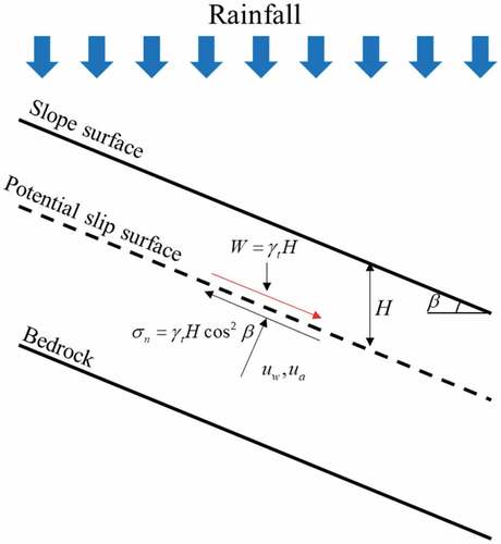
where H is the depth of the slip surface, $\beta$ is the angle of the slope, and ${\gamma }_t$ is the total unit weight of the soil.

3.2. Data

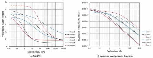
The daily rainfall data used in this study were measured at the Chiang Mai meteorological station (Station No. 48,327), which is operated by the Thai Meteorological Department. Daily rainfall data recorded from 1952 to 2019 were used in this study. The World Meteorological Organization (WMO) recommends using 30-year periods as a standard for summarizing climate trends (World Meteorological organization, 2017). Based on this recommendation, the analysis period was divided into two periods of 34 years: 1952 to 1985 and 1986 to 2019. The study considered six return periods, namely periods of 10, 25, 50, 100, 500, and 1,000 years, to create the IDF curve for extreme rainfall.  For soil properties, a database of residual soil properties was developed by Soralump and Thorwiwat (2009, 2010), and Thowiwat (2009) studied the physical and engineering properties, such as the grain size distribution, density, hydraulic properties and shear strength behavior, of residual soil in Thailand. For undisturbed and disturbed soil sampling, more than 500 samples were collected and tested in the laboratory to investigate the residual soil’s physical and engineering properties. The soil can be classified into nine groups based on the parent rock. The shear strength parameters for the analysis are shown in Table 1 and Figure 3. Figure 7 shows the SWCC and the hydraulic conductivity function. As described in the methods section, the SWCC and hydraulic conductivity function were estimated using the physicoempirical model developed by Arya and Paris and the closed-form equations derived by Van Genuchten. Elevation data were obtained from the ASTER Global Digital Elevation Model Version 3 (GDEM V3) collaboratively developed by the National Aeronautics and Space Administration (NASA) and the Ministry of Economy, Trade, and Industry of Japan (METI). The slope angle was derived from the 30-meter resolution version of the ASTER GDEM. The land use data were obtained from the Land Development Department of Thailand. The critical rainfall threshold for the early warning system was obtained from the Thailand Department of Water Resources.

Table 1. Cohesion of soil and friction angle values for different types of residual soil in Thailand (After Soralump, 2010).

Group	Parent rock for residual soil group	Cohesion of soil, kPa	Angle of friction, degree
1	Granite	11.87	28.25
2	Volcanic rock	18.34	22.90
3	Sandstone and Siltstone	14.51	27.49
4	Shale and Mudstone	13.83	25.98
5	Interbedded Sedimentary Rocks	10.29	28.52
6	Metamorphic Rock	11.38	30.13
7	Carbonate Rock
8	Quaternary deposits
9	Sedimentary Rock on Khorat Plateau

Figure 7. (a) SWCC and (b) hydraulic conductivity function.

4. Results and discussion

4.1. Changes in extreme rainfall

The analysis was based on the annual daily maximum rainfall data for Chiang Mai over 68 years. Figure 8 presents the annual daily maximum rainfall data from 1952 to 2019 and critical rainfall in the early warning system. The annual daily maximum rainfall data values were highly scattered, ranging from 35 to 166 mm. The study also performed a conventional trend analysis of the rainfall using regression equations – the best-fit equation was a sixth-order polynomial, and the corresponding value of the regression coefficient, R2, was 0.117. Table 2 shows the results of the conventional analysis of extreme rainfall using regression equations. The annual daily maximum rainfall data were divided into two periods: the first period was from 1952 to 1985 (blue bar in Figure 8), and the second period was from 1986 to 2019 (gray bar in Figure 8). By dividing the rainfall time series data into two periods, it found that the average annual daily maximum rainfall value during the first period was approximately 76.68 mm, whereas the value during the second period was approximately 85.23 mm. Thus, the average annual daily maximum rainfall increased by approximately 11.13% between the two periods.

Table 2. Results of conventional trend analysis of extreme rainfall using regression equations.

Trend type	Equation	R^2
Linear	y = 0.155 x – 226.6	0.013
Exponential	y = 0.977 e^0.0022x	0.018
Logarithmic	y = 308.67 ln(x) – 2263	0.013
Power	y = 3E-13 x^4.379	0.018
Second-order polynomial	y = −0.0074 x^2 + 29.729x – 29,584	0.022
Sixth-order polynomial	y = 2E-07 x^6 – 0.0029 × ^5 + 14.328 x^4 – 37,936 × ^3 + 6E+07 x^2 – 4E+10 x + 1E+13	0.117

Figure 8. Annual daily maximum rainfall from 1952 to 2019 and critical rainfall in the early warning system.

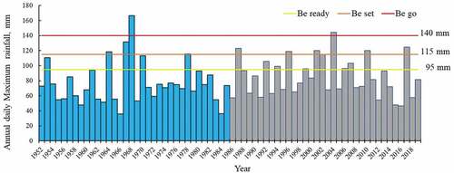
When comparing the annual daily maximum rainfall and the level of critical rainfall in the warning system of the Department of Water Resources, it found that there were 13 years in the second period during which the annual daily maximum rainfall value exceeded the threshold of the first level of the warning system (i.e. the “Be ready” level). In contrast, during the first period, there were only 7 years in which the annual daily maximum rainfall exceeded the threshold for the first level of the warning system. For the second level of the warning system (i.e. “Be set”), there were 7 years in the second period but only 4 years in the first period that reached this threshold. Thus, the increase in extreme rainfall in Chiang Mai Province also enhances the risk of landslides to the public in this area.

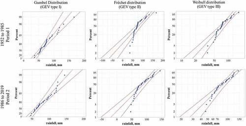
To analyze changes in the distribution of the annual daily maximum rainfall, the selection of the appropriate GEV is important. The AD test and the p value were used to verify the goodness-of-fit of the distribution; the H0 hypothesis was assumed that the data would follow the probability distribution at a significance level of 0.05. Based on these goodness-of-fit criteria, the GEV type 1 distribution (i.e. the Gumbel distribution) is the optimum distribution for fitting the rainfall data recorded at the Chiang Mai weather station. Table 3 lists the results of the goodness-of-fit tests, and Figure 9 presents the probability plots for both periods. According to the GEV analysis and the MLE data, the location and scale are the most significant distribution parameters. The value for the location for the first period (1952–1985) was 64.49, and the value for the second period (1986–2019) was 73.35. In addition, the scale value of the first period was 20.50; the equivalent value for the second period was 20.54. Based on these results, the annual daily maximum rainfall distribution changed significantly in terms of location but only comparatively slightly in scale. The change in the location of the distribution was approximately 13.7%.

Table 3. Results of goodness-of-fit tests for data recorded at the Chiang Mai weather station.

Goodness-of-fit metric	Data from 1952 to 1985 (First period)
	Gumbel distribution (GEV type I)	Fréchet distribution (GEV type II)	Weibull distribution (GEV type III)
AD	0.379	2.401	1.035
p-value	> 0.250	< 0.010	< 0.010
	Data from 1986 to 2019 (Second period)
AD	0.322	1.023	0.531
p-value	> 0.250	< 0.010	0.181

Figure 9. Probability plots for the annual daily maximum rainfall dataset.

Figure 10 shows the probability density and cumulative density functions for the two analyzed periods. A comparison of the extreme daily rainfall depth values for the return periods of 10, 25, 50, 100, 500, and 1,000 years showed that the rainfall intensity (mm per day) increased by approximately 9 mm for the investigated return period. The percentage of rainfall intensity increase was 9.78% for the 10-year return period, 8.41% for the 25-year return period, 7.63% for the 50-year return period, 6.98% for the 100-year return period, 5.85% for the 500-year return period, and 5.47% for the 1,000-year return period. Figure 11 shows the daily rainfall intensity for each return period investigated.

Figure 10. Probability density and cumulative density functions for two periods of analysis.

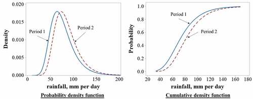
Figure 11. Rainfall intensity for daily rainfall for each investigated return period.

4.2. Changes in stability of residual soil slope

The pore water pressure is a key parameter for analyzing slope stability. In this study, pore water pressure profiles were simulated using extreme daily rainfall data obtained from rainfall analysis. The initial negative pore water pressure under hydrostatic conditions was taken to be approximately 50 kPa. After simulating the rainfall by using the value from IDF curves in each period and return period, the pore water pressure profiles indicated that the negative pore water pressure decreased to zero, with the rainfall intensity resulting in a positive pore water pressure at the sloping surface. The negative pore water pressure decreased with increased rainfall intensity due to the return period’s increase.

Furthermore, the soil matric suction increased with depth until it was reduced to hydrostatic conditions at a depth of 2 m. Figure 12 shows the pore water pressure profile for each group. A negative pore water pressure increases the shear strength of the residual soil slope and ensures that the soil slope is stabilized. High-intensity daily rainstorms can reduce the soil matric suction such that positive pore water pressure can be observed. Olivares and Picarelli (2003) proposed that a saturated soil slope with zero matric suction will be more susceptible to static liquefaction, which is the mechanism responsible for the occurrence of landslides. Hence, the safety factor decreased with the increase in rainfall intensity.

Figure 12. Pore water pressure profile in soil group one.

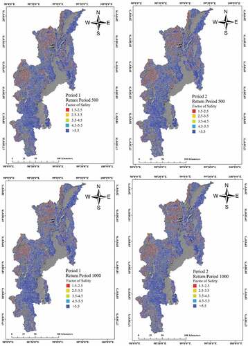
Figure 13 shows the factor of the safety map for each period as determined based on the return periods. Concerning the spatial distribution of the factor of safety, the results showed that the factor of safety was low in the mountainous area of the western region of Chiang Mai Province. In particular, the steep sloping surfaces surrounding the tops of mountains and valleys are critical zones. Concerning historical landslide events in Thailand, it has been reported that the steep slopes near the tops of mountains and the steep valleys are landslide susceptibility zones (Ono, Kazama, & Ekkawatpanit, 2014). When considering land use cases, it was found that forests and field crops and cultivation areas have a low safety factor. Finally, by comparing the factor of safety maps and the landslide susceptibility maps from the Department of Mineral Resources of Thailand, it found that there was good correspondence between the factor of safety maps and the landslide susceptibility maps from the Department of Mineral Resources of Thailand.

Figure 13. Safety map factor for each period based on various return periods.

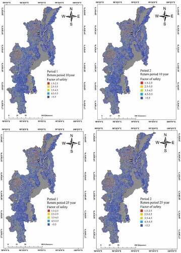
Figure 13. Continued.

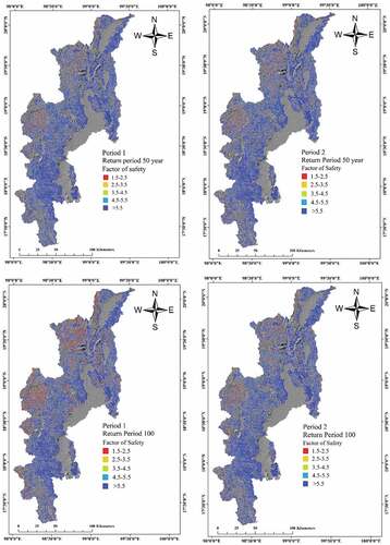
Figure 13. Continued.

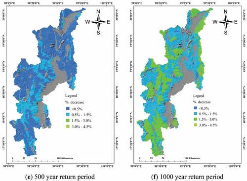
Figure 14 shows the map of the decrease in the safety factor from Period 1 to Period 2. A comparison of spatial distribution of safety factor values for Periods 1 and 2 showed that the safety factor was reduced by 0.02–4.5%. The spatial distribution of the decrease in the safety factor indicated that the decreases in the safety factor were not homogeneous. The decrease in the safety factor depends on the soil groups. The results indicated that the safety factor for soil Group 1 decreased significantly. Considering soil Group 1, it found that landslides occur the most commonly on this soil group type; moreover, soil Group 1 has the highest value of percentage of landslide occurrence frequency per area (Phattanaprateep, 2016; Soralump & Thorwiwat, 2009, 2010). The safety factor decreased significantly during the 1000-year return periods due to the significant reductions of unsaturated shear strength due to increased positive pore water pressure. Changes in pore water pressure are considered to be the key factor controlling slope stability (Nguyen & Likitlersuang, 2019; Ning & Godt, 2013)

Figure 14. Decrease in the safety factor o for each period based on various return periods.

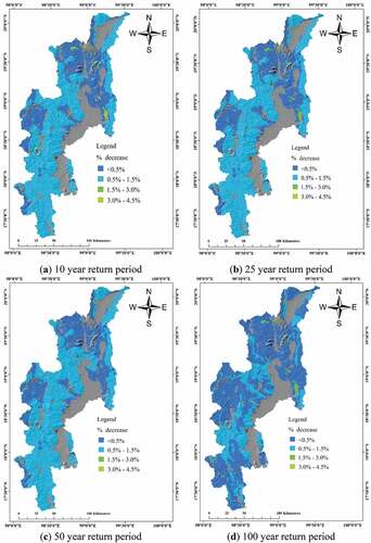
Figure 14. Continued.

5. Conclusions

In this study, the effects of changes in the distribution of extreme daily rainfall on the stability of residual soil slopes were investigated using a numerical model of rainfall-induced landslides. The primary conclusions of the study can be summarized as follows:

1. The main change that has occurred in the extreme daily rainfall distribution in the Chiang Mai province of Thailand is location, with a shift in the distribution curve toward the right. This means that Chiang Mai Province has experienced an increase in extreme rainfall events and the amount of heavy rainfall. An increase in heavy rainfall intensity may increase the frequency and magnitude of rainfall-related disasters, especially landslides.

2. The stability of the residual slope decreases with an increase in rainfall intensity. By comparing the slope stability for Periods 1 and 2 (i.e. 1952–1985 and 1986–2019), the study found that the safety factor of the slope decreased by 0.02–4.5% because the mean extreme daily rainfall value increased from Period 1 to Period 2. This reduction in the slope stability was not the same across the entire area or for all the soil groups but instead depended on the soil groups’ hydraulic properties and shear strength.

Although this study simulated the effects of the changes in the extreme daily rainfall distribution on the stability of the residual soil slope, several other triggering factors and causes of landslides that could also be considered. These include antecedent rainfall and combinations of factors such as heavy rainfall and earthquakes. Future research in this field could potentially address these aspects to gain further insights into landslide risk factors.

Acknowledgments

This research was supported by the Department of Geography, Faculty of Social Sciences, Kasetsart University. The authors gratefully acknowledge the rainfall data of the Thai Meteorological Department (TMD) and soil data of Geotechnical Engineering Research and Development Center, Department of Civil Engineering, Faculty of Engineering, Kasetsart University.

Disclosure statement

No potential conflict of interest was reported by the author(s).

Data availability statement

The data that support the findings of this study are available from the corresponding author, Thapthai Chaithong, upon reasonable request. https://drive.google.com/drive/folders/1HXMBMuQyUiK-Lm9DV6ArTFULymqee69h?usp=sharing

Additional information

Funding

This research was supported by the Department of Geography, Faculty of Social Sciences, Kasetsart University.

Notes on contributors

Thapthai Chaithong

Thapthai Chaithong is a lecturer in Department of Geography, Faculty of Social Sciences, Kasetsart University. He obtained his Ph.D. in Environmental Studies from Graduate School of Environmental Studies, Tohoku University, Japan. He obtained his M.Eng. in Civil Engineering from Kasetsart University, Thailand. He obtained his B.Eng. in Civil Engineering from King Monguk’s University of technology North Bangkok. His research interests include the development of analytical models for predicting landslide and debris flows, unsaturated soil behaviour, soil hydrology, and climate change. Now, his research focuses on the relation between changes in extreme climate (rainfall, temperature, and wind speed) and natural disasters.

References

- Arya, L. M., & Paris, J. F. (1981). A physicoempirical model to predict the soil moisture characteristic from particle-size distribution and bulk density data. Soil Science Society of America Journal, 45(6), 1026–1030.
- Chaithong, T. (2017). Analysis of extreme rainfall-induced slope failure using a rainfall infiltration-infinite slope analysis model. International Journal of GEOMATE, 13(35), 156–165.
- Chatra, A., Dodagoudar, G. R., & Maji, V. B. (2019). Numerical modelling of rainfall effects on the stability of soil slopes. International Journal of Geotechnical Engineering, 13(5), 425–437.
- Collins, B. D., & Znidarcic, D. (2004). Stability analyses of rainfall induced landslides. Journal of Geotechnical and Geoenvironmental Engineering, 130(4), 362–372.
- Cww, N., & Shi, Q. (1998). A numerical investigation of the stability of unsaturated soil slopes subjected to transient seepage. Computers and Geotechnics, 22(1), 1–28.
- Diaz, H. F., & Murnane, R. J. (2008). Climate extremes and society. United Kingdom: Cambridge University Press, Cambridge. doi:10.1017/CBO9780511535840.
- Eab, K. H., Likitlersuang, S., & Takahashi, A. (2015). Laboratory and modelling investigation of root-reinforced system for slope stabilisation. Soils and Foundations, 55(5), 1270–1281.
- Fredlund, D. G. (2006). Unsaturated soil mechanics in engineering practice. Journal of Geotechnical and Geoenvironmental Engineering, 132(3), 286–321.
- IPCC. (2021). Summary for policymakers. In Climate change 2021: The physical science basis. Contribution of working group I to the Sixth assessment report of the intergovernmental panel on climate change. Cambridge, United Kingdom: Cambridge University Press. (In Press).
- Jotisankasa, A., & Sawangsuriya, A. 2008 Application of unsaturated soil mechanics for slope stability. Paper presented at the 13rd National Convention on Civil Engineering, Thailand, Chonburi, May 14–16.
- Jotisankasa, A., Vathananukij, H., & Coop, M. 2009 Soil-water retention curves of some silty soils and their relations to fabrics. Paper presented at 4th Asia-Pacific Conference on Unsaturated Soils, Newcastle, Australia, November 23–55.
- Kodra, E., & Ganguly, A. R. (2014). Asymmetry of projected increases in extreme temperature distributions. Scientific Reports, 4(5884), 1–8.
- Li, W. C., Lee, L. M., Cai, H., Li, H. J., Dai, F. C., & Wang, M. L. (2013). Combined roles of saturated permeability and rainfall characteristics on surficial failure of homogeneous soil slope. Engineering Geology, 153, 105–113.
- Likitlersuang, S., Takahashi, A., & Eab, K. H. (2017). Modeling of root-reinforced soil slope under rainfall condition. Engineering Journal, 21(3), 123–132.
- Michel, G. P., Kobiyama, M., & Goerl, R. F. (2014). Comparative analysis of SHALSTAB and SINMAP for landslide susceptibility mapping in the Cunha River basin, southern Brazil. Journal of Soils and Sediments, 14(7), 1266–1277.
- Mishra, A. K., & Singh, V. P. (2010). Changes in extreme precipitation in Texas. Journal of Geophysical Research, 115(D14106), 1–29.
- Nadarajah, S. (2005). Extremes of daily rainfall in west central Florida. Climatic Change, 69(2–3), 325–342.
- National Academies of Sciences, Engineering, and Medicine. (2016). Attribution of extreme weather events in the context of climate change. Washington, DC: The National Academies Press.
- Nguyen, T. S., & Likitlersuang, S. (2019). Reliability analysis of unsaturated soil slope stability under infiltration considering hydraulic and shear strength parameters. Bulletin of Engineering Geology and the Environment, 78(8), 7527–5743. doi:10.1007/s10064-019-01513-2
- Nguyen, T. S., Likitlersuang, S., & Jotisankasa, A. (2019). Influence of the spatial variability of the root cohesion on a slope-scale stability model: A case study of residual soil slope in Thailand. Bulletin of Engineering Geology and the Environment, 78(5), 3337–3351.
- Nguyen, T. S., Likitlersuang, S., & Jotisankasa, A. (2020). Stability analysis of vegetated residual soil slope in Thailand under rainfall conditions. Environmental Geotechnics, 7(5), 338–349.
- Nguyen, T. S., Likitlersuang, S., Ohtsu, H., & Kitaoka, T. (2017). Influence of the spatial variability of shear strength parameters on rainfall induced landslides: A case study of sandstone slope in Japan. Arabian Journal of Geosciences, 10(16), 369.
- Ning, L., & Godt, J. W. (2013). Hillslope hydrology and stability. New York, United States of America: Cambridge University Press. Cambridge.
- Ning, L., & Griffiths, D. V. (2004). Profiles of steady-state suction stress in unsaturated soils. Journal of Geotechnical and Geoenvironmental Engineering, 130(10), 1063–1076.
- Oh, H. J., Lee, S., Chotikasathien, W., Kim, C. H., & Kwon, J. H. (2009). Predictive landslide susceptibility mapping using spatial information in the Pechabun area of Thailand. Environmental Geology, 57(3), 641–651.
- Olivares, L., & Picarelli, L. (2003). Shallow flow slides triggered by intense rainfalls on natural slopes covered by loose unsaturated pyroclastic soils. Géotechnique, 53(2), 283–287.
- Ono, K., Kazama, S., & Ekkawatpanit, C. (2014). Assessment of rainfall-induced shallow landslides in Phetchabun and Krabi provinces, Thailand. Natural Hazards, 74(3), 2089–2107.
- Park, J. S., Kang, H. S., Lee, Y. S., & Kim, M. K. (2011). Changes in the extreme daily rainfall in South Korea. Int J Climat, 31(15), 2290–2299.
- Phattanaprateep, S. 2016. Landslide hazard mapping by probabilistic approach based on uncertainty of soil property. Master Thesis, Kasetsart University, Bangkok.
- Phien-wej, N., Nutalaya, P., Aung, Z., & Zhibin, T. (1993). Catastrophic landslides and debris flows in Thailand. Bulletin of the International Association of Engineering Geology, 48(1), 93–100.
- Ragulina, G., & Reitan, T. (2017). Generalized extreme value shape parameter and its nature for extreme precipitation using long time series and the Bayesian approach. Hydrological Sciences Journal, 62(6), 863–879.
- Rahardjo, H., Li, X. W., Toll, D. G., & Leong, E. C. (2001). The effect of antecedent rainfall on slope stability. Geotechnical and Geological Engineering, 19(3/4), 371–399.
- Soralump, S. (2010). Rainfall-triggered landslide: From research to mitigation practice in Thailand. Geotechnical Engineering Journal of the SEAGS&AGSSEA, 41(1), 1–6.
- Soralump, S., & Thorwiwat, W., 2009. Shear strength behaviour of residual soil in Thailand subjected by changing in moisture content for supporting the landslide warning measure. Paper presented at the 14th National Convention on Civil Engineering, Thailand, Nakhon Ratchasima, May 13–15.
- Soralump, S., & Thorwiwat, W., 2010. Shear strength moisture behaviour of residua soils of landslide sensitive rocks group in Thailand. Paper presented at the 15th National Convention on Civil Engineering, Thailand, Ubon Ratchathani, May 12–14.
- Tan, Y. C., Ma, K. C., Chen, C. H., Ke, K. Y., & Wang, M. T. (2009). A numerical model of infiltration processes for hysteretic flow coupled with mass conservation. Irrigation and Drainage, 58(3), 366–380.
- Thowiwat, W. 2009. Critical API model for landslide warning of residual soils in Thailand. Master thesis, Kasetsart University.
- United Nations. 2021. The sustainable development goals report 2021. Author, New York, United States of America.
- Van Genuchten, M. T. (1980). A closed-form equation for predicting the hydraulic conductivity of saturated soils. Soil Science Society of America Journal, 44(5), 892–898.
- Wang, H., Sassa, K., & Fukuoka, H. (2003). Downslope volume enlargement of a debris slide-debris flow in the 1999 Hiroshima. Engineering Geology, 69(3–4), 309–330.
- World Meteorological organization. (2017). WMO Guildelines on the calculation of climate normal. Geneva, Switserland: World Meteorological Organiza-tion.
- Yilmaz, A. G., & Perera, B. J. C. (2014). Extreme rainfall nonstationarity investigation and intensity-frequency-duration relationship. Journal of Hydrologic Engineering, 19(6), 1160–1172.
- Zhang, L. L., Zhang, J., Zhang, L. M., & Tang, W. H. (2011). Stability analysis of rainfall-induced slope failure: A review. Proceedings of the Institution of Civil Engineers - Geotechnical Engineering, 164(GE5), 299–316.
- Zizioli, D., Meisina, C., Valentino, R., & Montrasio, L. (2013). Comparison between different approaches to modeling shallow landslide susceptibility: A case history in Oltrepe Pavese, Northern Italy. Natural Hazards and Earth System Sciences, 13(3), 559–573.