Beyond the SDG 15.3.1 Good Practice Guidance 1.0 using the Google Earth Engine platform: developing a self-adjusting algorithm to detect significant changes in water use efficiency and net primary production

ABSTRACT

Monitoring changes in Annual Net Primary Productivity (ANPP) is required for reporting on UN Sustainable Development Goal (SDG) Indicator 15.3.1: the proportion of land that is degraded over the total land area. Calibrating time-series observations of ANPP to derive Water Use Efficiency (WUE; a measure of ANPP per unit of evapotranspiration) can minimize the influence of climate factors on ANPP observations and highlight the influence of non-climatic drivers of degradation such as land use changes. Comparing the ANPP and WUE time series may be useful for identifying the primary drivers of land degradation, which could be used to support the Land Degradation Neutrality objectives of the UN Convention to Combat Desertification (UNCCD). This paper presents an algorithm for the Google Earth Engine (freely and openly available upon request – http://doi.org/10.5281/zenodo.4429773) to calculate and compare ANPP and WUE time series for Santa Cruz, Bolivia, which has recently experienced an intensification in its land use. This code builds on the Good Practice Guidance document (version 1) for monitoring SDG Indicator 15.3.1. We use the MODIS 16-day average, 250 m resolution to demonstrate that the Enhanced Vegetation Index (EVI) responds faster to changes in water availability than the Normalized Difference Vegetation Index (NDVI). We also consider the relationships between ANPP and WUE. Significant and concordant trends may highlight good agricultural practices or increased resilience in ecosystem structure and productivity when they are positive or reducing resilience and functional integrity if negative. The sign and significance of the correlation between ANPP and WUE may also diverge over time. With further analysis, it may be possible to interpret this relationship in terms of the drivers of change in plant productivity and ecosystem resilience.

KEYWORDS:

• Land degradation
• land productivity
• water use efficiency
• Google Earth Engine
• MODIS
• Good Practice Guidance
• SDG 15.3.1

1. Introduction

One of the key international frameworks aiming to ensure a sufficient balance between development ambitions and protection of the environment is the 2030 Agenda for Sustainable Development of the United Nations, which was adopted by all UN Member States in 2015 (United Nations, 2015). The 2030 Agenda includes 17 Sustainable Development Goals (SDGs) that countries are urged to address. UN SDG Goal 15 aims to “Protect, restore and promote sustainable use of terrestrial ecosystems, sustainably manage forests, combat desertification, halt and reverse land degradation and halt biodiversity loss”. Goal 15 comprises twelve Targets, including 15.3 which has the achievement of a land degradation neutral world by 2030 as one of its key objectives (Giuliani et al., 2020a; Sims et al., 2017).

Land Degradation Neutrality (LDN) is “a state whereby the amount and quality of land resources, necessary to support ecosystem functions and services and enhance food security, remains stable or increases within specified temporal and spatial scales and ecosystems” (Chasek et al., 2019; Cowie et al., 2018). Efforts to achieve LDN are supported by the LDN Program of the UN Convention to Combat Desertification (UNCCD; the custodian agency of SDG Target 15.3) to which 123 countries have agreed to set LDN Targets, and the LDN Initiative of the Group on Earth Observations (GEO LDN - http://earthobservations.org/geo_ldn.php) which assists countries to build analytical and on-ground capacity to address land degradation, identify datasets suitable for calculating LDN and develop analytical tools to improve the measurement of land degradation for calculating and reporting on LDN and the SDG (Giuliani et al., 2020b).

For both LDN and UN SDG Target 15.3, the extent of land degradation is measured using a single indicator: 15.3.1, which reports the extent of land that is degraded over total land area per country. The UNCCD has produced two versions of the Good Practice Guidance document (GPG; Sims et al., 2017, 2021) describing methods for calculating UN SDG Indicator 15.3.1 and its three sub indicators which are as follows: (1) land cover and land cover change; (2) land productivity and (3) carbon stocks (above and below ground) which are currently represented by the surrogate of soil organic Carbon (SOC) stocks. The methods presented in the GPG version 1 have facilitated the elevation of SDG Indicator 15.3.1 to SDG Tier 1, reflecting that it has an internationally agreed methodology that is being used by countries to report on the indicator.

To identify the different drivers of degradation it was suggested (but not specifically implemented) to compare and co-interpret time series of ANPP data, such as the Normalized Difference Vegetation Index (NDVI; Tucker, 1979) or the Enhanced Vegetation Index (EVI; Didan, Munoz, Solano, & Huete, 2015; Huete et al., 2002), against a time series of plant productivity data that has been transformed to indicate water use efficiency, such as the Water Use Efficiency (WUE) algorithm presented by Steduto, Hsiao, Fereres, and Raes (2012). This information may help countries to plan actions to avoid further land degradation or to restore degraded areas as they strive to achieve LDN (Sims, Barger, Metternicht, & England, 2020). Nevertheless, such comparison, to the best of our knowledge, has never been done.

Consequently, the aim of this paper is to present an implementation of the methods for calculating the land productivity sub-indicator of SDG Indicator 15.3.1, as described in the GPG version 1, using an open source, self-adjusting algorithm developed in Google Earth Engine (GEE): a cloud-based satellite data processing platform (Gorelick et al., 2017). The methodology is applied on a twenty-year time series of MODIS data collected over the Santa Cruz Department in Bolivia to demonstrate the application and outputs of this algorithm. Agricultural activity has increased in this region over recent decades, and there is now evidence of significant land degradation which may pose a threat to the integrity of its unique biodiversity (Verdum, Gamboa, & Bebbington, 2018) and increase the risk of extensive wildfires, such as those observed in 2019 which were attributed to inappropriate agricultural practices and policies.¹ SDG Indicator 15.3.1 and the LDN activities provide a well-established mechanism for Bolivia to monitor the condition of its land resources as it strives to implement its economic development objectives.

2. Land productivity and its relationship with water use efficiency

The GPG version 1 describes the computation of three metrics of land productivity degradation, which are combined to determine the land productivity sub-indicator. The metrics are (1) Trend, which measures the change in productivity levels over the long term, (2) State, which compares recent productivity in a local area to its long-term average, and (3) Performance, which compares local productivity to productivity in other areas with a similar land cover type and productivity potential. These metrics are adapted from the World Atlas of Desertification (WAD), developed by the European Commission’s Joint Research Centre (JRC) to measure land degradation at global scales (Ivits & Cherlet, 2016).

To assess whether land productivity degradation patterns are statistically significant, the GPG version 1 recommends assessing the significance of the long-term Trend using Z-scores to assess the steepness of the slope, and P-values to determine the probability that observed spatial patterns are created by random processes. Z-scores and P-values are associated with standard normal distribution, with very high or low Z-scores in conjunction with low P-values indicating that the observed spatial pattern is significant and did not occur by chance. The GPG version 1 recommends that significance be identified at the P-values ≤0.05 level, with Z-scores defining degradation groupings as shown below:

• Z < −1.96 = Potential degradation, as indicated by a significant decreasing trend

• Z > −1.96 AND <1.96 = No significant change

• Z > 1.96 = Potential improvement, as indicated by a significant increasing trend

The GPG version 1 describes the potential benefits of deriving a productivity time series from two Annual Net Primary Productivity (ANPP) time series; a “raw” series showing all changes in productivity regardless of the drivers and an ANPP time series that has been transformed to show Water Use Efficiency (WUE; Ponce Campos et al., 2013), expressed as follows: the amount of carbon assimilated as biomass or grain produced per unit of water used by the crop (Hatfield & Dold, 2019). Variations in the raw ANPP time series are typically strongly influenced by variations in moisture availability (Le Houerou, 1984; Wessels et al., 2007), whereas these effects are reduced in the WUE time series.

Calibrating the ANPP time series to minimize climate effects is a highly contentious subject, with some Earth Observation (EO) specialists insisting that calibration should always be performed and others insisting that it should never be (GEO-LDN Initiative, 2020). The view presented in the GPG version 1 is that each of these time series potentially highlights different drivers of degradation. The ANPP time series is strongly influenced by variations in water availability such as drought and the effects of climate change, whereas the WUE time series may highlight impacts from more direct anthropogenic activities such as land use changes. A reduction in land productivity arising from either of these suites of drivers constitutes land degradation in the context of SDG Indicator 15.3.1. Calculating both ANPP and WUE time series may provide the ability to evaluate land degradation impacts from these different drivers, which may provide critical information to support the determination of appropriate remediation activities or to avoid further degradation.

Ponce Campos et al. (2013) describe the calculation of Ecosystem Water Use Efficiency (WUE_E) as the ratio of ANPP to evapotranspiration (ET), defined as precipitation minus the water lost to surface runoff, recharge to groundwater and changes to soil water storage. They demonstrate a near-linear relationship between ANPP and ET across grassland and forest biomes in the United States, Puerto Rico and Australia, and an identical relationship has also been identified for crops (Steduto, Hsiao, Fereres, & Raes, 2012).

WUE_E calibration is performed by calculating the ratio of ANPP to ET observations integrated over the same period as the productivity observations each year. WUE_E correction appears to be the most hydrologically comprehensive and widely applicable of the rainfall calibration methods described in the GPG version 1. Ponce Campos et al. (2013) integrated evapotranspiration over calendar years, which ignores variations in the timing of peak biomass and rainfall per year and may be inappropriate in southern hemisphere temperate regions where the growing season may span the change of year. A more dynamic approach is to accumulate evapotranspiration up to the month of peak biomass as formulated by Steduto, Hsiao, Fereres, and Raes (2012). Consequently, the method we adopted for calculating annual WUE_E is (Equation (1)(1) $\mathrm{W}\mathrm{U}\mathrm{E}\mathrm{E}=\frac{\mathrm{A}\mathrm{N}\mathrm{P}\mathrm{P}}{\sum \mathrm{E}\mathrm{T}}$(1) ):

(1) $\mathrm{W}\mathrm{U}\mathrm{E}\mathrm{E}=\frac{\mathrm{A}\mathrm{N}\mathrm{P}\mathrm{P}}{\sum \mathrm{E}\mathrm{T}}$(1)

3. Study area: the Santa Cruz Department in Bolivia

In recent decades, the production of agricultural commodities has significantly increased in the Bolivian lowlands (Figure 1). The Santa Cruz Department is considered the breadbasket of Bolivia, but agricultural development has historically been restricted by financial and policy restrictions. A history of continual weakening of nature conservation frameworks and institutions, combined with record low prices for hydrocarbons (Bolivia’s primary source of revenues, see Ducoing et al., 2018) has inspired a diversification into agricultural commodities, which may pose risks to the integrity of Bolivia’s unique biodiversity (Verdum, Gamboa, & Bebbington, 2018). Recent policy changes are paving the way for increased national and international investment in Bolivian agricultural enterprises, with the likelihood of significant increases in development levels throughout the country in the short to medium term (Supreme Decree 4272, 24th of July 2020²).

Figure 1. The Santa Cruz Department in Bolivia, South America.

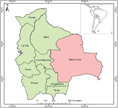
Agricultural activity in the Santa Cruz Department of this region has particularly intensified to supply a growing national market for animal products and grains from the eastern plains and mountainous regions, and fruits and vegetables from the mesothermic valleys in the west (Muller, Pacheco, & Montero, 2014; Steininger et al., 2002).

4. Method and implementation

The GPG version 1 identifies the following key challenges to improve the consistency of measurement of the sub-indicator on Land Productivity globally. These are:

1. Identifying the best proxy for plant productivity

2. Selection of the period of peak biomass

3. Calculation of growing season metrics

4. Selection of the best evapotranspiration datasets for comparison with productivity time series

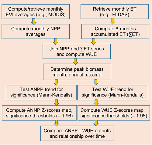
To tackle these four challenges, the proposed workflow (Figure 2) has been implemented as a JavaScript code in the Google Earth Engine to retrieve 16-day Moderate Resolution Imaging Spectroradiometer (MODIS) Vegetation Index data at 250 m resolution from both AQUA (MYD13Q1) and TERRA (MOD13Q1) missions and compile the selected images into NDVI and EVI monthly means representing net primary productivity for each month. MODIS data were selected for their free availability, global coverage, dense time series and long data archive. The monthly NPP means are then appended to ET data accumulated over a 6-month period to calculate ∑ET. The month of peak biomass per year is calculated independently from the month of peak WUE. Details for each of these key challenges are described in the following sub-sections.

Figure 2. Graphical summary of the main processing steps implemented in GEE.

4.1. Identifying the best-fit proxy for NPP

NDVI is presented throughout GPG version 1 as the default vegetation index to be used in the absence of information to justify the use of an alternative index (GEO-LDN Initiative, 2020). The NDVI is a combination of red and near-infrared (NIR) wavelengths that are sensitive to green vegetation biomass and growth vigor (Equation (2)(2) $\mathrm{N}\mathrm{D}\mathrm{V}\mathrm{I}=\frac{\left(NIR-RED\right)}{\left(NIR+RED\right)}$(2) ).

(2) $\mathrm{N}\mathrm{D}\mathrm{V}\mathrm{I}=\frac{\left(NIR-RED\right)}{\left(NIR+RED\right)}$(2)

The NDVI is presented as the default proxy of primary productivity in the GPG version 1 because it is probably the best-known vegetation index, it can be calculated from many Earth observation satellite sensors, nevertheless shortcomings include a tendency to saturate in high biomass areas, and the potential sensitivity to variations in the brightness of the background material (Huete, Liu, Batchily, & van Leeuwen, 1997). There are many alternatives to the NDVI described in the literature (Bao, Li, Gu, & Liu, 2019; FAO, 2012; Jarchow, Didan, Barreto-Muñoz, Nagler, & Glenn, 2018; Jay, Potter, & Crabtree, 2016; Liang, Cui, Feng, Wang, & Xia, 2009; Ponce Campos et al., 2013; Potter, Gross, & Genovese, 2007; Wang et al., 2019; Wang, Niu, Yang, & Zhou, 2010; Yang, Fang, Ji, & Han, 2009a; Yang, Fang, Pan, & Ji, 2009b). In particular, the Enhanced Vegetation Index (EVI; Didan, Munoz, Solano, & Huete, 2015) is recommended in the GPG version 1 for use in high biomass areas (Equation (3)(3) $\mathrm{E}\mathrm{V}\mathrm{I}=2.5\times \frac{\left(\mathrm{N}\mathrm{I}\mathrm{R}-\mathrm{R}\mathrm{E}\mathrm{D}\right)}{\left(\mathrm{N}\mathrm{I}\mathrm{R}+\hspace{0.17em}6\times \mathrm{R}\mathrm{E}\mathrm{D}-7.5\times \mathrm{B}\mathrm{L}\mathrm{U}\mathrm{E}+\hspace{0.17em}1\right)}$(3) ):

(3) $\mathrm{E}\mathrm{V}\mathrm{I}=2.5\times \frac{\left(\mathrm{N}\mathrm{I}\mathrm{R}-\mathrm{R}\mathrm{E}\mathrm{D}\right)}{\left(\mathrm{N}\mathrm{I}\mathrm{R}+\hspace{0.17em}6\times \mathrm{R}\mathrm{E}\mathrm{D}-7.5\times \mathrm{B}\mathrm{L}\mathrm{U}\mathrm{E}+\hspace{0.17em}1\right)}$(3)

The EVI is less sensitive to saturation in high biomass regions than the NDVI, but the inclusion of the blue wavelengths in the EVI precents it being calculated from several global datasets.

This study compares the NDVI and the EVI, and assesses their correlation to variations in evapotranspiration as a test of their suitability for assessing WUE (see Figure 4). EVI is available as 16-days moving average product in Google Earth Engine (merging TERRA and AQUA datasets, the time granule increases to 8-days moving average), reducing computation significantly. The EVI removes soil-brightness induced variations and decouples the soil and atmospheric influences from the vegetation signal by including a feedback term for simultaneous correction (Didan, Munoz, Solano, & Huete, 2015). Most importantly to this study, our preliminary analysis indicated that EVI responds more quickly to changes in moisture levels than the 2-band EVI (EVI2; Jiang, Huete, Didan, & Miura, 2008) which eliminates the blue band. Consequently, we focused this comparison between the 3-band EVI and the NDVI, both of which are available as standardized MODIS products.

4.2. Selection of a peak biomass month

GPG version 1 recommends calculating productivity Trend using the annual productivity maxima or productivity observed at the same time each year in areas where cloud cover might prevent observation of the land surface using satellite EO data, for instance. The adaptive noise filtering method can improve the precision of selecting the peak biomass growth period by capturing a peak biomass month for each pixel.

The period of peak biomass is selected by first calculating monthly averages of NDVI and EVI, and then calculating 1-month and 3-month moving averages from these data (Figure 3). ET accumulation (and hence the growing season) is considered to start when the 1-month and 3-month moving average time series cross at their minima. The growing season is considered to end at the month of peak biomass indicated by the 1-month moving average values, with the month of peak accumulated value representing the annual maximum NPP.

Figure 3. Growing season averaged for Santa Cruz, Bolivia showing the 1-month (blue line) and 3-month (yellow line) moving average EVI values, and showing the growing season (red box).

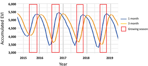
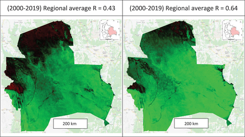
Figure 4. NDVI (left) and EVI (right) monthly correlation with evapo-transpiration (FLDAS), correlation: green=1; black=0; red=−1.

Precipitation in Santa Cruz from 2000 to 2019 is at its most between December and January, on average. In addition to variations in cloud cover, spatial and temporal patterns of rainfall and growing conditions, there have also been many changes in land use and land cover in Bolivia which mean that peak biomass can differ from time and place in any given year. Consequently, there is no single peak biomass period across the studied region. Each pixel has its own unique ANPP and WUE trajectories, which may change each year. Rather than identifying an arbitrary period, there is a need to identify individual annual NPP maxima adaptively.

Monthly WUE is calculated independently from the ET data producing two parallel time-series of annual maxima. Sen’s slope is applied to each of these time series, and the Mann–Kendall test is applied to the Sen’s regression line to determine the direction and significance of change in both parameters. A two-pass filter including the calculation of monthly cloud-masked means which are subsequently filtered to generate a mosaic of local annual maxima was then used to improve the representation of peak biomass.

4.3. Selection of growing season metrics

The GPG version 1 describes the use of Timesat (Jönsson & Eklundh, 2004; Tan et al., 2011) to extract the vegetation index data over the growing season, which is done using either fixed dates or parameters measured from the NPP time series itself. Improved precision in selecting the time series over which these data are measured should also improve the accuracy of WUE calibration.

Peak growing seasons that tend to occur early in the calendar year can complicate the process of identifying the peak ANPP per year. Thus, the design of a self-adjusting algorithm to select the most appropriate growing season metrics and identify annual WUE maxima on a per-pixels basis is more challenging than demonstrated for vegetation indices, which have no carry-over of information from 1 year to the next. Peak biomass is straightforwardly identified and selected to build annual maxima mosaics. Generating a self-adjusting growing season metrics for higher precision required more steps.

4.4. Selection of an evapotranspiration dataset to calculate WUE

We aggregated the MODIS NDVI and EVI datasets to monthly time series and selected the evapotranspiration dataset that was most highly correlated to the MODIS indices for further analysis. According to our tests, the Famine Early Warning Systems Network (FEWS NET) Land Data Assimilation System evapotranspiration datasets (FLDAS; McNally et al., 2017), published as monthly granules, are the best option. Even if monthly Climate and Climatic Water Balance for Global Terrestrial Surfaces (TerraClimate; Abatzoglou, Dobrowski, Parks, & Hegewisch, 2018) appear to be of interest, both spanning longer than MODIS’s two decades, TerraClimate’s datasets require longer processing time and have a coarser spatial resolution of 2.5 arc minutes against 0.1 degrees for FLDAS. Moreover, as of June 2020, TerraClimate’s evapotranspiration for 2019 was not available. These considerations make the FLDAS dataset more useful for fast-tracking of SDG 15.3.1.

FLDAS and TerraClimate ET datasets proved to be best fit for the purpose of WUE trend analysis using a data-driven approach, while TerraClimate shows better statistics it only covers up to 2018 in GEE, thus FLDAS is the best available choice to fast-tracking WUE to qualify ANPP Land Trend Productivity.

5. Results

To validate the technical feasibility, identify possible issues and determine the potential of such approach, the proposed workflow has been tested over the Santa Cruz region in Bolivia.

5.1. Productivity dynamics

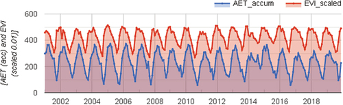
The NDVI and EVI time series exhibit annual maxima early in the calendar year (Figure 5), which correlates with the period of peak rainfall in this area. Averaged over the 20 years between 2000 and 2019, NDVI peaks around DOY55 and EVI around DOY24. Peak NDVI therefore typically lags peak EVI by about 1 month, which we interpret as a faster response to variations in moisture levels of the EVI compared to the NDVI. The relationship between evapotranspiration and EVI over the time series used in this analysis is shown in Figure 6.

Figure 5. MODIS retrieved NDVI and EVI median by DOY in Santa Cruz, Bolivia (2001–2020).

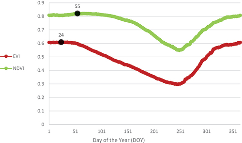
Figure 6. MODIS retrieved EVI monthly median in Santa Cruz, Bolivia (2001–2020).

5.2. Comparison of ANPP and WUE

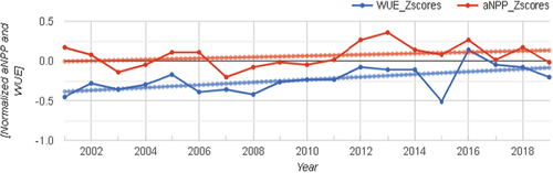
There is a weak but significant positive correlation between ANPP and WUE Mann-Kendall significance Z scores (R² = 0.18, Figure 7) over the 20 years from 2001 to 2020, while the comparison of normalized trends (Figure 8) shows that there has been a slight reduction in annual primary productivity and a marked increase in water use efficiency as a product of adaptation to decreasing precipitation in a context of fast land use changes.

Figure 7. Comparing ANPP and FLDAS-derived WUE Mann-Kendall significance.

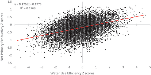
Figure 8. Comparing normalized ANPP and FLDAS-derived WUE Sen’s slope.

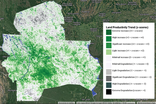
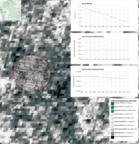
Figure 9 shows the spatial distribution of changes in ANPP over time (i.e. not corrected to account for water use efficiency). Areas with a strong increase in ANPP are often located adjacent to watercourses such as the Parapetí river running NE-SW in the western region of the map, a semi-arid region beneficiary of irrigation projects. In contrast to WUE (Figure 9), distinct areas of decrease in ANPP are evident (Figure 9), showing the impact of disturbances such as selective logging, fire, agricultural conversion and urbanization, and reductions in ANPP evident in Figure 9 (shown in black) are mainly driven by factors other than moisture availability. Increasing WUE (Figure 10) indicates that vegetation in these areas may be adapting to convert available moisture more efficiently into plant biomass over this time, which can be interpreted as a resilient response.

Figure 9. Spatial distribution of ANPP Sen’s slope trend significance in Santa Cruz, Bolivia (2001–2020).

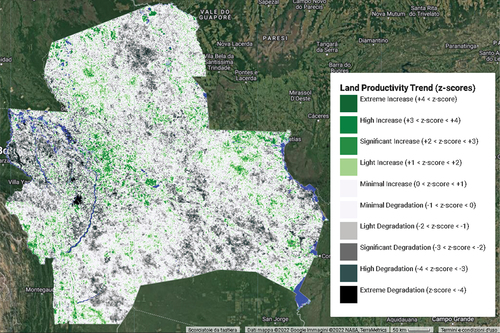
Figure 10. Spatial distribution of WUE Sen’s slope trend significance in Santa Cruz, Bolivia (2001–2020).

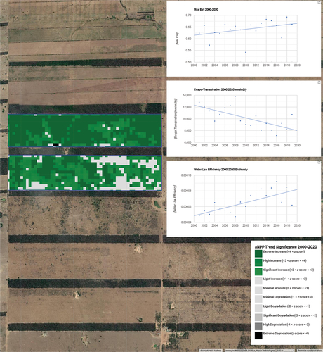
Below are three interpreted examples of use cases for the algorithm: 1. ANPP is decreasing alongside, with WUE as an example of steady land degradation following overgrazing on two selected paddocks (Figure 11). 2. aNPP and WUE show concomitant improvement on a different piece of grazeland, due to improved management (Figure 12). Both properties have been deforested and used for grazing before 2000. It is common to observe declining primary productivity as the water input declines, while WUI (the response to the water input) tends to increase as a resilient response to a changing climate, up to a certain point. Figures 11 and 12 show two special cases: the worst-case and the best-case scenarios. Despite the declining water input shown in the evapotranspiration charts (common in most of the Santa Cruz Department), in one case the paddocks’ carrying capacity was systematically surpassed leading to progressive land degradation in terms of primary productivity and water use efficiency (Figure 11). In example 2 more careful grazing management led to increased land and water productivity (Figure 12).

Figure 11. ANPP and WUE degradation following deforestation and overgrazing (30 m).

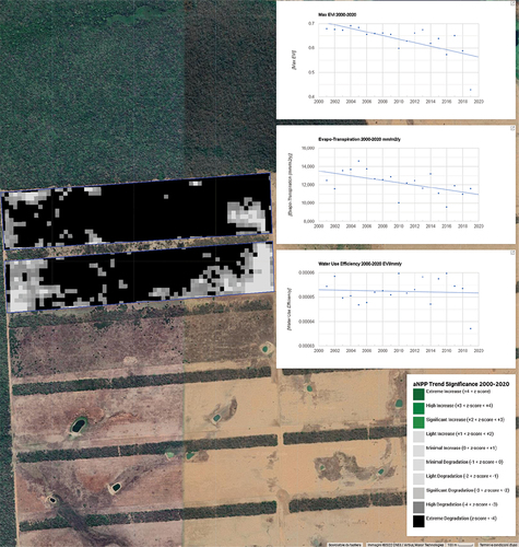
Figure 12. ANPP and WUE improvement following better grazeland management (30 m).

A third example shows a forested area where the main driver of land degradation is climate change: both NPP and WUE declined steadily over the past two decades (Figure 13). While reduced primary productivity is a natural response to a declining water input, the adaptive response of healthy vegetation is to increase the water productivity in an attempt to retain function despite adverse environmental changes. Following Ponce Campos et al. (2013), the declining WUE is an indicator of resilience loss at the level of the ecosystem. Declining trends in both indicators, NPP and WUE, clearly identify vegetation communities at risk.

Figure 13. ANPP and WUE degradation in a forested area, northern Santa Cruz-Bolivia (250m and 30m).

6. Discussion

A range of datasets are potentially suitable for collection images throughout the growing season in this region, with the principal ones being MODIS (TERRA and AQUA), with daily repeat coverage for some data products and a smallest pixel resolution 250 m, Sentinel 2 which captures five to six repeat coverages per month at a resolution as small as 10 m in some wavelengths, and the Landsat satellites which have a repeat coverage every 16 days and a pixel size of 30 m. Each of these datasets provide time-series throughout the growing season that have differences in their data density, spatial resolution, and cloud contamination, which impacts the likelihood of imaging the moment of peak biomass in the relatively high-frequency MODIS and Sentinel 2 datasets. The lower frequency Landsat datasets are also affected by the scan line correction failure on Landsat 7, which creates data gaps in Landsat 7 scenes.

Consistent and representative data describing ANPP are critical for accurately measuring and monitoring the extent of land productivity degradation in the context SDG Indicator 15.3.1 and LDN. Extracting these data from noisy time-series affected by many biotic and abiotic factors can be challenging and time-consuming. This proposed methodology simplifies this process. In addition, it facilitates the comparison of trends in ANPP and WUE, which can be used to interpret different drivers of degradation, and the structural and functional integrity of ecological and agricultural systems.

Despite the data smoothing methods applied here, some noise remaining in the data may affect the results of this analysis. Grazed land and short-cycle multi-crop systems, with two or more harvests per year are a common example, but also minor fire disturbances affecting the canopy represent highly likely contingencies. Under some conditions, this noise may cause errors in WUE estimation, however we estimate that these errors are less significant than the errors likely to be introduced by an inaccurate selection of peak growing period from the time series data.

While water use efficiency represents the “cost” in terms of water use to produce biomass, it is also informative about the resilience of agricultural and ecological systems: the ability to retain growth function despite water stress or in other words the inelasticity of carbon capture versus water used.

It may be argued that a poor or negative correlation between NPP and WUE outcomes is more informative than a high correlation. A strong positive correlation may be expected where plant growth is matched by increases in WUE, which may occur throughout the lifecycle of certain plant species. A negative correlation may indicate that more biomass is being produced (positive ANPP Z-scores) at a higher water use (negative WUE Z-scores) or that ecosystems or crop systems may reduce above ground biomass production adaptively responding to a drying climate (negative ANPP Z-scores) making a more efficient use of scarce water (positive WUE Z-scores).

While high agreement between loss of both ANPP and WUE can unambiguously be interpreted as land degradation, the relationship between WUE and ANPP is highly variable and often very low. The interpretation of this relationship, at times negative, requires further study to determine the meaning of discrepancies and corresponding courses of action for practitioners and land managers: i.e. a loss of ANPP is associated with an increase in WUE may reveal a process of adaptation to a drying climate, while the opposite condition may be associated with sub-optimal land uses. While improving WUE may reveal successful adaptation of ecological and agricultural systems, significantly degrading WUE could represent a serious early warning of ecological collapse, representing a loss of resilience.

Reduced NPP is a sign of degradation, but increased WUE may be a sign of “Ecosystem resilience despite large-scale altered hydroclimatic conditions” (Ponce Campos et al., 2013). NPP is maintained despite a reduced water input; in this case, ecosystems resilience is understood as the ability of the ecosystem to retain biomass growth function under unfavorable climate conditions. Some ecosystems change in response to water stress with reduced plant size, making better use of water. This is both a degradation in terms of NPP and a resilient adaptation. If an ecosystem loses both NPP and WUE, it may be approaching collapse, and WUE would then represent an important ancillary data that help to qualify and quantify changes in land productivity. This result is one original bit of contribution to the field.

Crop irrigation is still uncommon in Santa Cruz, so the improvement in water use efficiency can be attributed mostly to ecosystems' response to climate trends and improvements in land management in selected grassland and cropland. Comparing WUE trends to ANPP trends reveals an interesting aspect of vegetation: while total greenness and biomass productivity decline the efficiency in using scarce water in a changing climate may increase. Specific WUE early warning products may be designed to assist in the identification, decision-making process, and monitoring of degraded or at-risk ecosystems for the UN Decade on Restoration (2021–2030) https://www.decadeonrestoration.org/. The tool developed and published alongside this paper already belongs to such class. The drivers leading to poor or negative correlations between these factors should be investigated further.

While it is recognized that MODIS may be too coarse for accurate representation of ANPP distribution in small countries or regions, the MODIS datasets provided the best utility in our analytics system. While every run of the MODIS script generated a global dataset, with Landsat 4–8 and Sentinel 2 the GEE limit of 5000 images was quickly met, demanding more time to generate a global dataset or simply comparable datasets covering the study period in a given area of interest. The highest resolution and precision may be attained with a Sentinel 1 and 2 combined NPP index, while it is still too early to generate a meaningful time series, the 2030 final assessment of the UN Decade on Restoration (2021–2030) may benefit from a uniquely fine-grained dataset already within the reach of minor adaptation in our code. Recent experiences with data cubes (Giuliani et al., 2020a, 2020b) also represent good practices that might be translated to JavaScript for a single-stop solution and universal application in countries that monitor SDG 15.3.1. Making all the computation directly in GEE provides the benefit of a faster and simpler generation of results, with a lower entry barrier and reduced steepness of the learning curve for in-country personnel. Ownership of the diagnostic results may be enhanced through a single-stop technical solution for national staff, reducing time and cost of specialized training.

7. Conclusions

For the purposes of calculating SDG Indicator 15.3.1, the sub-indicator of plant condition is ANPP. The present exploration of how ANPP and WUE land productivity trends relate to each other was inspired by the GPG version 1, which proposes that a comparison between WUE and ANPP time-series might be used to identify different drivers of degradation, but which does not process this interrogation in depth. This paper has demonstrated that EVI is superior to NDVI for this comparison and presented an automated system for calculating the appropriate growing season metrics to simplify and standardise this analysis for all potential users.

While a reduction of both ANPP and WUE (indicating a reduction in both the growth vigor and efficiency of water use) can generally be interpreted as land degradation, in practice the relationship between WUE and ANPP over time is highly variable and often poorly correlated. A loss of ANPP with corresponding increase in WUE may indicate increasing ecosystem resilience despite large-scale altered hydroclimatic conditions (Ponce Campos et al., 2013). Alternatively, an increase in ANPP with a corresponding reduction in WUE may indicate unsustainable land use or management practices or intensity. Further work is required to comprehend the full complexity of the interaction between these two parameters, identify specific climate, land use and land management drivers that lead to those outcomes, and interpret the appropriate courses of action to avoid, reduce or remediate negative outcomes based on these data.

The algorithm presented in this paper enables trends in ANPP and WUE to be easily compared, within the general framework provided by the GPG version 1 for reporting on the land productivity sub-indicator of SDG 15.3.1. To that end, a self-adjusting algorithm was developed using the Google Earth Engine platform to virtually eliminate the need for parametrization that works with a range of freely available global satellite EO datasets. The Santa Cruz Department of Bolivia was chosen to test the tool due to its renowned biodiversity and significant land use changes. Future work comparing changes in WUE and ANPP, supplemented by information on changes in climatic, land management and land use conditions in Santa Cruz, could be used to further validate the approach presented in the GPG version 1 and in this paper.

Acknowledgments

This study was partially funded by UNDP Grant: BOL/118208 (“Laboratorios de Recuperación Temprana”), a study led by Fundación para Conservación del Bosque Chiquitano (www.fcbc.org.bo) to determine forest patches requiring post-fire assisted recovery in the aftermath of 2019 wildfires in Santa Cruz, Bolivia: “Plan Estratégico para la Restauración de las Áreas Afectadas por los Incendios en el 2019”.

Disclosure statement

No potential conflict of interest was reported by the author(s).

Data availability statement

The data that support the findings of this study are openly available on the Google Earth Engine at: https://developers.google.com/earth-engine/datasets.

Additional information

Notes on contributors

Andrea Markos

Andrea Markos is an experienced Spatial Analyst with a trajectory in the non-profit sector supporting food security, rural development, and natural resources management. His current challenges consist in providing precision grazing services to livestock producers and predictive services as well as technical assistance to Governments in fire modelling, monitoring, and management in the South American region.

Neil Sims

Neil Sims is a highly experienced leader of large and complex national and international projects. His background is in the use of remote sensing methods to monitor changes in plant growth responses over time. His projects have included writing methods to help countries report on the United Nations Sustainable Development Goals (UNSDGs) and developing methods for biosecurity monitoring crop diseases from satellites. His current challenge is adapting the Australian-developed Open Data Cube technology to meet the needs of Small Island Developing States (SIDS) countries in the Pacific Region to support their resource management needs, including reporting on the UNSDGs.

Gregory Giuliani

Gregory Giuliani is the Head of the Digital Earth Unit and Swiss Data Cube Project Leader at GRID-Geneva of the United Nations Environment Programme (UNEP) and a Senior Lecturer at the University of Geneva’s Institute for Environmental Sciences. He is a geologist and environmental scientist who specializes in Remote Sensing, Geographical Information Systems (GIS) and Spatial Data Infrastructures (SDI). He also works at GRID-Geneva of the United Nations Environment Programme (UNEP) since 2001, where he was previously the focal point for Spatial Data Infrastructure (SDI) and is currently the Head of the Digital Earth Unit. Dr. Giuliani’s research focuses on Land Change Science and how Earth observations can be used to monitor and assess environmental changes and support sustainable development.

Notes

1. https://cnnespanol.cnn.com/2019/10/15/los-incendios-de-la-chiquitania-tendria-impacto-en-el-voto-de-los-bolivianos/

2. https://www.asfi.gob.bo/images/MARCO_NORMATIVO/SERV_FINAN_/D.S._4272.pdf

References

- Abatzoglou, J. T., Dobrowski, S. Z., Parks, S. A., & Hegewisch, K. C. (2018). Terraclimate, a high-resolution global dataset of monthly climate and climatic water balance from 1958–2015. Scientific Data, 5(1), 170191. doi:10.1038/sdata.2017.191
- Bao, N., Li, W., Gu, X., & Liu, Y. (2019). Biomass estimation for semiarid vegetation and mine rehabilitation using worldview-3 and sentinel-1 SAR imagery. Remote Sensing, 11(23), 2855. doi:10.3390/rs11232855
- Chasek, P., Akhtar-Schuster, M., Orr, B. J., Luise, A., Rakoto Ratsimba, H., & Safriel, U. (2019). Land degradation neutrality: The science-policy interface from the UNCCD to national implementation. Environmental Science & Policy, 92, 182–190. doi:10.1016/j.envsci.2018.11.017
- Cowie, A. L., Orr, B. J., Castillo Sanchez, V. M., Chasek, P., Crossman, N. D., Erlewein, A., & Welton, S. (2018). Land in balance: The scientific conceptual framework for Land Degradation Neutrality Environ. Environmental Science & Policy, 79, 25–35. doi:10.1016/j.envsci.2017.10.011
- Didan, K., Munoz, A. B., Solano, R., & Huete, A. (2015). MODIS vegetation index user’s guide (MOD13 Series) version 3.00, June 2015 (collection 6). Retrieved from https://lpdaac.usgs.gov/documents/103/MOD13_User_Guide_V6.pdf
- Ducoing, C., Peres-Cajías, J., Badia-Miró, M., Bergquist, A. -K., Contreras, C., Ranestad, K., & Torregrosa, S. (2018). Natural resources curse in the long run? Bolivia, Chile and Peru in the Nordic Countries’ mirror. Sustainability, 10(4), 965. doi:10.3390/su10040965
- FAO. (2012). Conducting national feed assessments. In Michael B. Coughenour & Harinder P.S. Makkar. FAO Animal Production and Health Manual No. 15. Rome, Italy.
- Fensholt, R., Rasmussen, K., Kaspersen, P., Huber, S., Horion, S., & Swinnen, E. (2013). Assessing land degradation/recovery in the African Sahel from long-term earth observation based primary productivity and precipitation relationships. Remote Sensing, 5(2), 664. doi:10.3390/rs5020664
- Funk, C., Peterson, P., Landsfeld, M., Pedreros, D., Verdin, J., Shukla, S., … Michaelsen, J. (2015). The climate hazards infrared precipitation with stations—a new environmental record for monitoring extremes. Scientific Data, 2(1), 150066. doi:10.1038/sdata.2015.66
- GEO-LDN Initiative. (2020). Minimum data quality standards and decision trees for SDG Indicator 15.3.1: Proportion of land that is degraded over total land area. In Technical Note. Group on Earth observation land degradation neutrality (GEO-LDN). Geneva, Switzerland: Initiative. Retrieved from http://earthobservations.org/documents/ldn/20200703_GEOLDN_TechnicalNote_FINAL_SINGLE.pdf
- Giuliani, G., Chatenoux, B., Benvenuti, A., Lacroix, P., Santoro, M., & Mazzetti, P. (2020a). Monitoring land degradation at national level using satellite earth observation time-series data to support SDG15 – exploring the potential of data cube. Big Earth Data, 4(1), 3–22. doi:10.1080/20964471.2020.1711633
- Giuliani, G., Mazzetti, P., Santoro, M., Nativi, S., Van Bemmelen, J., Colangeli, G., & Lehmann, A. (2020b). Knowledge generation using satellite earth observations to support Sustainable Development Goals (SDG): A use case on land degradation. International Journal of Applied Earth Observation and Geoinformation, 88, 102068. doi:10.1016/j.jag.2020.102068
- Gorelick, N., Hancher, M., Dixon, M., Ilyushchenko, S., Thau, D., & Moore, R. (2017). Google earth engine: Planetary-scale geospatial analysis for everyone, remote sensing of environment. (Vol. 202, pp. 18–27). ISSN 0034-4257. doi:10.1016/j.rse.2017.06.031
- Hatfield, J. L., & Dold, C. (2019). Water-use efficiency: Advances and challenges in a changing climate. Frontiers in Plant Science. doi:10.3389/fpls.2019.00103
- Huete, A. R., Liu, H. Q., Batchily, K., & van Leeuwen, W. (1997). A comparison of vegetation indices over a global set of TM images for EOS-MODIS. Remote Sensing of Environment, 59(3), 440–451. doi:10.1016/S0034-4257(96)00112-5
- Huete, A., Didan, K., Miura, T., Rodriguez, E. P., Gao, X., & Ferreira, L. G. (2002). Overview of the radiometric and biophysical performance of the MODIS vegetation indices. Remote Sensing of Environment, 83(1–2), 195–213. doi:10.1016/S0034-4257(02)00096-2
- Ivits, E., & Cherlet, M. (2016). Land productivity dynamics: Towards integrated assessment of land degradation at global scales. Luxembourg: Joint Research Centre.
- Jarchow, C. J., Didan, K., Barreto-Muñoz, A., Nagler, P. L., & Glenn, E. P. (2018). Application and comparison of the MODIS-derived enhanced vegetation index to VIIRS, Landsat 5 TM and Landsat 8 OLI Platforms: A case study in the Arid Colorado River Delta, Mexico. Sensors (Basel), 18(5), 1546. doi:10.3390/s18051546
- Jay, S., Potter, C., & Crabtree, R. (2016). Evaluation of modelled net primary production using MODIS and Landsat satellite data fusion. Carbon Balance and Management, 11(1). doi:10.1186/s13021-016-0049-6
- Jiang, Z., Huete, A. R., Didan, K., & Miura, T. (2008). Development of a two-band enhanced vegetation index without a blue band. Remote Sensing of Environment, 112(10), 3833–3845. doi:10.1016/j.rse.2008.06.006
- Jönsson, P., & Eklundh, L. (2004). Timesat—A program for analyzing time-series of satellite sensor data. Computers & Geosciences, 30(8), 833–845. doi:10.1016/j.cageo.2004.05.006
- Le Houerou, H. N. (1984). Rain use efficiency: A unifying concept in arid-land ecology. Kidlington, ROYAUME-UNI: Elsevier.
- Liang, T., Cui, X., Feng, Q., Wang, Y., & Xia, W. (2009). Remotely sensed dynamics monitoring of grassland aboveground biomass and carrying capacity during 2001–2008 in Gannan pastoral area. Acta Prataculturae Sinica, 18, 12–22.
- Ma, X., Huete, A., Moran, S., Ponce Campos, G., & Eamus, D. (2015). Abrupt shifts in phenology and vegetation productivity under climate extremes. Journal of Geophysical Research: Biogeosciences, 120(10), 2036–2052. doi:10.1002/2015JG003144
- McNally, A., Arsenault, K., Kumar, S., Shukla, S., Peterson, P., Wang, S., … Verdin, J. P. (2017). A land data assimilation system for sub-Saharan Africa food and water security applications. Scientific Data, 4(1), 170012. doi:10.1038/sdata.2017.12
- Muller, R., Pacheco, P., & Montero, J.C. (2014). The context of deforestation and forest degradation in Bolivia: Drivers, agents and institutions. In Occasional paper 108. Bpogor, Indonesia: CIFOR.
- Ponce Campos, G. E., Moran, M. S., Huete, A., Zhang, Y., Bresloff, C., Huxman, T., … Starks, P. J. (2013). Ecosystem resilience despite large-scale altered hydroclimatic conditions. Nature, 494(7437), 349–352. doi:10.1038/nature11836
- Potter, C., Gross, P., & Genovese, V. (2007). Net primary productivity of forest stands in New Hampshire estimated from Landsat and MODIS satellite data. Carbon Balance and Management, 2(1). doi:10.1186/1750-0680-2-9
- Rodell, M., Houser, P. R., Jambor, U., Gottschalck, J., Mitchell, K., Meng, C. J., … Toll, D. (2004). The global land data assimilation system. Bulletin of the American Meteorological Society, 85(3), 381–394. doi:10.1175/BAMS-85-3-381
- Sims, N., Green, C., Newnham, G.J., England, J.R., Held, A., Wulder, M., … McKenzie, N. 2017 Good practice guidance SDG indicator 15.3.1 proportion of land that is degraded over total land area. Version 1. Retrieved from https://www.unccd.int/sites/default/files/relevant-links/2017-0/Good%20Practice%20Guidance_SDG%20Indicator%2015.3.1_Version%201.0.pdf
- Sims, N. C., Barger, N. N., Metternicht, G. I., & England, J. R. (2020). A land degradation interpretation matrix for reporting on UN SDG indicator 15.3.1 and land degradation neutrality. Environmental Science & Policy, 114, 1–6. doi:10.1016/j.envsci.2020.07.015
- Sims, N. C., Newnham, G. J., England, J. R., Guerschman, J., Cox, S. J. D., Roxburgh, S. H., … Wheeler, I. (2021). Good practice guidance. SDG indicator 15.3.1, proportion of land that is degraded over total land area. version 2.0. Bonn, Germany: United Nations Convention to Combat Desertification. Retrieved from https://www.unccd.int/publications/good-practice-guidance-sdg-indicator-1531-proportion-land-degraded-over-total-land
- Steduto, P., Hsiao, T. C., Fereres, E., & Raes, D. (2012). Crop yield response to water. FAO Irrigation and Drainage Paper Nr. 66. Rome, Italy. Retrieved from http://www.fao.org/docrep/016/i2800e/i2800e00.htm
- Steininger, M. K., Tucker, C. J., Ersts, P., Killeen, T. J., Villegas, Z., & Hecht, S. B. (2002). Clearance and fragmentation of tropical deciduous forest in the Tierras Bajas. Santa Cruz, Bolivia. doi:10.1046/j.1523-1739.2001.015004856
- Tan, B., Morisette, J. T., Wolfe, R. E., Gao, F., Ederer, G. A., Nightingale, J., & Pedelty, J. A. (2011). An enhanced TIMESAT algorithm for estimating vegetation phenology metrics from MODIS data. IEEE Journal of Selected Topics in Applied Earth Observations and Remote Sensing, 4(2), 361–371. doi:10.1109/JSTARS.2010.2075916.
- Tucker, C. J. (1979). Red and photographic infrared linear combinations for monitoring vegetation. Remote Sensing of Environment, 8(2), 127–150. doi:10.1016/0034-4257(79)90013-0
- Verdum, R., Gamboa, C., & Bebbington, A.J. (2018). Assessment and scoping of extractive industries and infrastructure in relation to deforestation: Amazonia. Retrieved from http://www.climateandlandusealliance.org/wp-content/uploads/2020/03/Amazonia-Report-EN-FINAL-w-cover.pdf
- Wang, L. A., Niu, K. C., Yang, Y. H., & Zhou, P. (2010). Patterns of above- and belowground biomass allocation in China’s grasslands: Evidence from individual-level observations. Science China Life Sciences, 53(7), 851–857. doi:10.1007/s11427-010-4027-z
- Wang, J., Xiao, X., Bajgain, R., Starks, P., Steiner, J., Doughty, B. R., & Chang, Q. (2019). Estimating leaf area index and aboveground biomass of grazing pastures using Sentinel-1, Sentinel-2 and Landsat images. ISPRS Journal of Photogrammetry and Remote Sensing, 154, 189–201. doi:10.1016/j.isprsjprs.2019.06.007
- Wessels, K. J., Prince, S. D., Malherbe, J., Small, J., Frost, P. E., & VanZyl, D. (2007). Can human-induced land degradation be distinguished from the effects of rainfall variability? A case study in South Africa. Journal of Arid Environments, 68(2), 271–297. doi:10.1016/j.jaridenv.2006.05.015
- Yang, Y. H., Fang, J. Y., Ji, C. J., & Han, W. X. (2009a). Above- and belowground biomass allocation in Tibetan grasslands. Journal of Vegetation Science, 20(1), 177–184. doi:10.1111/j.1654-1103.2009.05566.x
- Yang, Y. H., Fang, J. Y., Pan, Y. D., & Ji, C. J. (2009b). Aboveground biomass in Tibetan grasslands. Journal of Arid Environments, 73(1), 91–95. doi:10.1016/j.jaridenv.2008.09.027