Area and shape distortions in open-source discrete global grid systems

ABSTRACT

A Discrete Global Grid System (DGGS) is a type of spatial reference system that tessellates the globe into many individual, evenly spaced, and well-aligned cells to encode location and, thus, can serve as a basis for data cube construction. This facilitates integration and aggregation of multi-resolution data from various sources to rapidly calculate spatial statistics. We calculated normalized area and compactness for cell geometries from 5 open-source DGGS implementations - Uber H3, Google S2, RiskAware OpenEAGGR, rHEALPix by Landcare Research New Zealand, and DGGRID by Southern Oregon University - to evaluate their suitability for a global-level statistical data cube. We conclude that the rHEALPix and OpenEAGGR and DGGRID ISEA-based DGGS definitions are most suitable for global statistics because they have the strongest guarantee of equal area preservation - where each cell covers almost exactly the same area on the globe. Uber H3 has the smallest shape distortions, but Uber H3 and Google S2 have the largest variations in cell area. However, they provide more mature software library functionalities. DGGRID provides excellent functionality to construct grids with desired geometric properties but as the only implementation does not provide functions for traversal and navigation within a grid after its construction.

KEYWORDS:

• Coordinate reference systems
• spatial indexing
• big spatial data analytics
• data cube
• DGGS

1. Introduction

In the last decade, the rapid increase in Earth Observation data accumulation and the trend towards open data have made a vast variety of high quality, high resolution, globally covering data available. Several petabytes of geospatial data occupy servers around the world and more continues to be generated every day (Alderson, Purss, Du, Mahdavi-Amiri, & Samavati, 2020). In the era of Big Data and ongoing globalization, the scientific community, the public sector, and industry need to analyze spatial data and overcome challenges related to processing enormous amounts of data. To unify concepts for such spatio-temporal gridded data, data cubes are often used nowadays (Giuliani et al., 2017; Lewis et al., 2017). However, current data cube implementations are fundamentally based on a singular projected coordinate system, meaning that users have to choose one-fits-all purpose. de Sousa, Poggio, Luis, Poggio, and Kempen (2019) examined the five most common global equal-area projections available in GIS software: Sinusoidal, Eckert, Homolosine, Mollweide and Hammer. They found that although these projections provide a significantly better spatial representation for global raster-based datasets, compared to the well-known Mercator projection, they still have area and shape distortions distributed throughout the projection surface. Moreover, some of these global equal-area projections are still poorly implemented in open-source geoprocessing libraries (de Sousa, 2018).

Another approach is to introduce a multi-projection system with individual projection parameters for continental regions, such as the Equi7 Grid (Bauer-Marschallinger, Sabel, & Wagner, 2014). The Equi7 Grid divides the globe into seven zones, which align with the continents, and defines customized equidistant azimuthal projections for each of these zones. The oversampling factor for Equi7 Grid, which the authors describe as the effects of resampling data when projecting satellite imagery from geographic into a projected coordinate reference system, is very low, a desirable property for data storage purposes (Bauer-Marschallinger, Sabel, & Wagner, 2014). However, such approaches create their own challenges, such as the computational overhead of managing different projections simultaneously, and the overlap between various Cartesian spaces at the boundaries between the zones (de Sousa, 2018).

Traditional spatial data models for accessing and analyzing spatial information are becoming inadequate due to the global extent (Breunig et al., 2020; Li et al., 2020). To efficiently analyze these massive volumes of data, it is important to provide them in a seamless interoperable format without the necessity to perform transformations from one cartographic projection to another (Baumann, 2021; de Sousa, Poggio, Luis, Poggio, & Kempen, 2019; Seong, Mulcahy, & Usery, 2002). Besides being computationally expensive, reprojecting introduces additional artifacts and uncertainties. Hence, classic Cartesian grid-based data representations should be considered outdated, imprecise, and not suitable for the full spectrum of global data analyses (Baumann, 2021).

Discrete Global Grid Systems (DGGS) are increasingly considered as a globally applicable reference system and spatial data model for congruent hierarchical data cubes and spatial data generally (Goodchild, 2018; Mahdavi-Amiri, Alderson, & Samavati, 2015; Purss et al., 2019; Yao et al., 2020). A DGGS discretizes the surface of the Earth into a set of regular cells (tessellation) onto the faces of a base solid, typically a polyhedron such as a cube or an icosahedron. These cells are geo-referenced and addressed with an indexing mechanism to assign and retrieve data. Most systems described in the literature are based on a) the cube as the base solid, b) quaternary triangular meshes an icosahedron base solid, c) or hexagonal systems on an icosahedron base solid (Gray, 1995; Mahdavi-Amiri, Harrison, & Samavati, 2014; Sahr, 2011; Snyder, 1992).

The recent interest in DGGSs among remote sensing and geospatial experts has likely gained momentum due to the overall maturing of geospatial technologies, the location-based and earth observation data accumulation in general (Guo, 2017), and the emergence of effective DGGS-based software products in various domains in particular (Bondaruk, Roberts, & Robertson, 2020; Bowater & Wachowicz, 2020; Hojati, Robertson, Roberts, & Chaudhuri, 2022; Purss, Gibb, Samavati, Peterson, & Ben, 2016; Robertson, Chaudhuri, Hojati, & Roberts, 2020). The terminology for such systems has been refined over the decades: hierarchical tessellations (Dutton, 1989), hierarchical spatial data structures (Goodchild & Shiren, 1992), recursive tessellations of the globe (White, 2000; White, Kimerling, Sahr, & Song, 1998), and now, with an Open Geospatial Consortium (OGC) specification recently being introduced, global grid systems have been established as “ … a spatial reference system that uses a hierarchical tessellation of cells to partition and address the globe. DGGSs are characterized by the properties of their cell structure, geo-encoding, quantization strategy and associated mathematical functions” (Open Geospatial Consortium, 2017). DGGS-based GIS analyses are already being conducted across a variety of domains, including crime analysis (Jendryke & McClure, 2019), wildfire modeling (Robertson, Chaudhuri, Hojati, & Roberts, 2020), flood mapping (Chaudhuri, Gray, & Robertson, 2021), characterization of coastal environments (Bousquin, 2021), and risk analysis for marine traffic (Rawson, Sabeur, & Brito, 2021). Various large-scale GIS challenges are being reevaluated on DGGS, including watershed delineation, land use/land cover change statistics, and general earth system modeling (Liao, Tesfa, Duan, & Leung, 2020; Lin, Zhou, Xu, Zhu, & Lu, 2018; Montibeller, Kmoch, Virro, Mander, & Uuemaa, 2020). Such studies rely on available open-source DGGS implementations and authors state unanimously that DGGS are favorable geospatial frameworks for data integration and large-scale environmental modeling and analysis.

Li and Stefanakis (2020) summarized the advantages of DGGS against traditional GIS. However, cell divisions of DGGS implementations have different geometric properties due to the choice of the base solid, tessellation scheme, and geographic referencing or projection method for the cells. Depending on the DGGS implementation, the area and shape-preserving properties can vary slightly. These are the most important properties when dealing with spatial data and calculating spatial statistics. Therefore, it is essential to identify which DGGS implementations are the best for preserving area and shape properties.

White, Kimerling, Sahr, and Song (1998) calculated various density ratios and reported that tessellations based on the icosahedron generally performed better than other base solids, and that the ISEA projection performed the best in terms of area distortion, and the Gnomonic projection performed the best on compactness. Kimerling, Sahr, White, and Song (1999) calculated spheroidal surface area, compactness, and centerpoint spacing and confirmed that icosahedral ISEA-based DGGSs are promising, in particular with triangular and hexagonal tessellations. Gregory, Kimerling, White, and Sahr (2008) described an inter-cell distance metric where Fuller – Gray DGGSs performed well, and shape-preserving equal-angle DGGSs performed surprisingly worse. Finally, Lei, Qi, and Tian (2020) defined the Zone Standardized Compactness, similar to the spherical compactness of Kimerling, Sahr, White, and Song (1999), and compared their novel coordinate system, which is based on spherical area coordinates (SACs) on various base polyhedra with triangular tessellations, to classic DGGSs, including ISEA and Fuller-Gray. They conclude that their DGGS has a generally smoother distribution in both area and shape distortions.

Open-source DGGSs have not been compared and evaluated comprehensively in terms of area and shape-preserving properties. We address that by comparing areal equality and compactness of the cell geometries of open-source icosahedron- and cube-based hierarchical and congruent DGGSs across several levels of resolution. In addition, we conduct all analyses from a practical perspective by integrating readily available open-source DGGS software with the Python programming language into a workflow to identify which DGGS implementation has the smallest area and shape distortions.

The article is structured as follows: In Section 2.1 we describe the open-source software packages. Then we describe the reproducible experimental setup in Section 2.2. Then we report and visualize the results in Section 3. We conclude the article with a discussion and outlook. We provide Jupyter notebooks, Python libraries and the generated data via open-access repositories (Kmoch & Vasilyev, 2022a, 2022b).

2. Methodology

2.1. Open-source DGGS implementations

2.1.1. Uber H3

The Hexagonal Hierarchical Geospatial Indexing System (H3) was developed at Uber as a grid system for optimization of ride pricing and dispatch, for visualizing and exploring spatial data, especially focusing on cities (Uber Technologies Inc, 2018). In 2018, Uber open-sourced their H3 C-library and it was rapidly adopted by the geospatial community. Currently there are implementations of the H3 library for all popular programming languages, even for native querying in data base management systems like Google BigQuery and PostgreSQL. The underlying DGGS of the H3 library is based on an aperture 7 hexagonal tessellation of the icosahedron. The Dymaxion orientation of the base icosahedron (Gray, 1995) was chosen based on the company’s business needs – all vertices are placed in the ocean to minimize distance distortions in cities. H3 uses the Gnomonic projection, which preserves shape well but incurs significant distortions of areas (Kimerling, Sahr, White, & Song, 1999). However, the centers of each cell have the same distance to the centers of all adjacent cells, thus, H3 hexagons are well suited for modeling of movements through the grid. Two indexing methods are used: (1) axis-based for indexing the cells on the planar faces of the icosahedron, and (2) a hierarchical indexing, which reliably expresses the parent-child-relationships of cells across the different resolutions, which always means exactly seven children relate to one parent cell and are approximately congruent. Combining the two indexing schemes allows flexible and computationally efficient methods for neighboring and hierarchical traversing (Bondaruk, Roberts, & Robertson, 2020; Li & Stefanakis, 2020).

2.1.2. Google S2

Another well-developed and widely used open-source package with DGGS capabilities is the S2 Geometry library, developed by Google engineers (Veach et al., 2017). The core library is written in C++, with software libraries available for Python, Java, JavaScript, R, and others at varying levels of maturity. The primary purpose of S2 is to provide operations for computational geometry and spatial indexing on the sphere. S2 uses the cube as the base polyhedron with a fixed orientation. Two faces are located with their centroids on the poles, one face having its centroid on the intersection of the prime meridian and the equator, and the other faces evenly surrounding the equator. The chosen tessellation shape for the cube is the square with a fully congruent aperture 4 refinement. For indexing, a Hilbert space-filling curve (Hamilton & Rau-Chaplin, 2008; Hilbert, 1891) is used to recursively index the cells for all resolutions on the six faces of the cube. Apart from numerous methods for spherical geometry operations, S2 provides conversion methods from geographic coordinates to cells and back for grid traversal (Bondaruk, Roberts, & Robertson, 2020; Li & Stefanakis, 2020).

2.1.3. RiskAware OpenEAGGR

RiskAware developed and published the Open Equal Area Global Grid (OpenEAGGR) library in 2017 (Bush, 2017). The OpenEAGGR library is written in C++ with available programming interfaces for Python, C and Java. The library currently supports two DGGS implementations, both use an icosahedron as the base solid and the ISEA projection, but different tessellation shapes: 1) ISEA4T, with a hierarchical equilateral triangle grid with aperture 4 with hierarchical indexing, and b) ISEA3H, a hexagonal grid of aperture 3 with offset coordinate cell indexing (Bush, 2017). The programming interface provides functions to convert to and from geographic coordinates and methods for spatial analysis such as intersections and proximity. The OpenEAGGR ISEA4T DGGS is based on a fully congruent hierarchical triangle tessellation (4 child triangles perfectly subdividing a parent triangle). However, the ISEA3H DGGS implementation is not congruent, only supports offset indexing, and does not support hierarchical or unique identifier-based indexing (Bondaruk, Roberts, & Robertson, 2020; Li & Stefanakis, 2020).

2.1.4. rHEALPix

The rearranged Hierarchical Equal Area isoLatitude Pixelization (rHEALPix) DGGS is based on the HEALPix system (Gorski, Hivon, & Wandelt, 1998) and it has a base solid as cube (Gibb, Raichev, & Speth, 2016). As the tessellation shape, four variations are used depending on the latitude – a quad cell (quadrilateral), a dart cell (triangular), a skew-quad cell (quadrilateral), and a cap cell (circular). All 4 shapes are congruent and form an aperture 9 refinement. rHEALPix uses a custom projection with the same name as the implementation and it preserves the area. Gibb, Raichev, and Speth (2016) emphasize that the projection is non-conformal and does not preserve the shape of cells well, but its original intention was to achieve equal-area cells throughout all resolutions. For indexing, Z (Morton) space-filling curves are used for every face of the cube. The rHEALPix implementation is currently only available as a Python package and provides functionality like conversion to and from geographic coordinates and grid traversing (Bowater & Stefanakis, 2018; Li & Stefanakis, 2020).

2.1.5. DGGRID

DGGRID is an open-source command-line application written in C++ (Sahr, 2019). In contrast to the previously described software packages, DGGRID allows the construction of various icosahedral DGGSs rather than focused usage of a particular one. The functionality of the application allows to define tessellation shape (triangles, diamonds, hexagons), orientation, and projection method (ISEA or Fuller-Gray), a resolution, and area of interest. DGGRID only operates with the icosahedron as the base polyhedron, and its core functionality revolves around binning point data into DGGS cells at a chosen resolution (Sahr, 2008, 2011). DGGRID exports generated DGGS to standard GIS formats. Several software packages provide convenient wrappers to use the tool programmatically, the most prominent being dggridR for the R Statistical language (Barnes, 2018). Several Python packages are available as well (Correndo, 2019; Hojati, 2019; Kmoch, 2020).

2.2. Comparison of the geometric properties of open-source DGGS implementations

Kimerling, Sahr, White, and Song (1999) suggest that comparisons of geometric properties for global grids should at least consider surface area and compactness. These metrics should be calculated for all cells at the same level of the grid resolution. However, as the selected DGGSs use different apertures, tessellation schemes (e.g. triangle, quads, hexagons) and even base solids (icosahedron, cube), the corresponding resolution levels varied for the different DGGS and could only be compared at closest approximate cell sizes. We decided to select a range of resolutions for each DGGS, from coarse (resolution 2) to a resolution containing at most 400,000 cells, corresponding to an average cell size of 1500 to 3000 $k{m}^2$ (Table 1). The metrics were calculated for individual cells and results stored as associated attributes together with index and geometry.

Table 1. Evaluated software packages and DGGS types, selected resolution levels and corresponding maximum number of cells at the highest resolution.

Software	DGGS type	Aperture	Tessellation	Resolutions	Max no. cells
H3	H3	7	Hexagon	2-4	284,649
S2	S2	4	Square	2-8	388,775
OpenEAGGR	ISEA4T	4	Triangle	2-7	323,391
rHEALPix	rHEALPix	9	Multiple	2-5	349,548
DGGRID	ISEA7H	7	Hexagon	2-5	165,957
DGGRID	FULLER7H	7	Hexagon	2-5	165,956
DGGRID	ISEA4D	4	Diamond	2-7	161,796
DGGRID	FULLER4D	4	Diamond	2-7	161,796
DGGRID	ISEA4T	4	Triangle	2-7	323,644
DGGRID	FULLER4T	4	Triangle	2-7	323,644

Values were standardized to a standard scale to compare the different metrics across the DGGSs. Following Kimerling, Sahr, White, and Song (1999), to check for equal area, all cell areas were normalized by dividing by the mean area of all cells at the same resolution. For a genuinely equal-area DGGS implementation, the value should be as close to 1 as possible. For area comparison between resolution levels, standard deviation and range were also calculated.

Compactness measures the complexity of a polygon, typically by comparing it against the perimeter of a circle with the same area (Li, Goodchild, & Church, 2013). Among many alternatives, the isoperimetric inequality (IPQ) compactness measure has become one of the most widely accepted (Osserman, 1978). The metric is unitless and varies between 0 and 1. A circle is the most compact shape, with a compactness measure of 1, and as shapes become more complex and less compact, their measure decreases towards zero.

(1) $C_{IPQ}=\frac{4\pi A}{p^2}$(1)

where A is the cell area and p is the cell perimeter (Osserman, 1978).

All investigated implementations provide a programming interface for the Python language. A set of Python scripts have been developed to increase reusability and to integrate these with Python’s geospatial libraries, i.e. Geopandas (Jordahl & Contributors, 2021). The source code was made accessible under an open-source license (Kmoch & Vasilyev, 2022a).

Table 1 lists the tested configurations and the maximum number of cells in a global coverage for each DGGS of the highest selected resolution. Directly comparing the resolution levels between different DGGSs is not meaningful. However, within a single DGGS, the change in the overall number of cells when switching to the next higher (or lower) is always a multiple of the aperture. Thus, it is not possible to try achieving identical cell sizes. Most DGGSs allow resolutions with an average cell size down to or even below $m^2$. DGGRID provides several more variations, including aperture 3 and 4 hexagonal tessellations. We do not include those because they are not congruent and, thus, not immediately practical to use in use for a data cube.

We used the following workflow for every DGGS implementation:

1. Generate global coverage cells for selected resolutions and create cell geometries in WGS84 coordinates and saved as Parquet-files;

2. Remove cells with invalid geometry where areas are not calculated correctly, such as those that cross the dateline;

3. Calculate cell area and perimeter in planar units. Reproject each cell individually into the Lambert Azimuthal Equal Area projection using the cell centroid as the origin of the projection; converted to FlatGeoBuf spatial data format for post-processing and archiving;

4. Calculate standardized area and compactness for every cell using area and perimeter from the previous step;

H3, S2, and OpenEAGGR only implement fixed orientation configurations for the DGGS. DGGRID and rHEALPix provide configuration parameters for the orientation of the base solid. In these cases, we only generated the cells for the default configuration, i.e. no additional parameters were used, and we used the WGS84_003 default ellipsoid setting for rHEALPix. We calculated cell area, perimeter, standardized area, and standardized compactness for the planar cell geometries and stored these as additional attributes. We visualized the results as maps and histograms (cf. Appendix A1).

3. Results

3.1. Spatial and statistical distribution of standardized cell area and compactness

All data is made accessible as summary spreadsheets (Tables A1 and A2), maps and histograms (Figures A1 to A10), as well as intermediate processing data files as supplements (Kmoch & Vasilyev, 2022b).

3.1.1. Uber H3

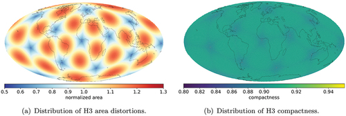
Figure 1(a) shows clearly that H3 DGGS cells do not have an equal area across the whole global tessellation. The distortions follow the geometry of the underlying icosahedron, and the area changes from the central parts of the faces to the edges. The biggest difference occurs between cells lying closer to the centers of the faces and cells at the vertices, almost varying up to $\pm 50$%, with a large standard deviation for the normalized area metric of 0.13. This is the consequence of using the Gnomonic projection for the faces of the icosahedron. This distribution follows the pattern described by Kimerling, Sahr, White, and Song (1999). However, cell shapes are well-preserved with some minor distortions in compactness at the icosahedron’s vertices (Figure 1b). These distortions then rapidly even out towards the faces forming almost a uniform overall pattern. It should be noted for completeness that in all hexagonal DGGS, there exist a small number of pentagons on the joint corners of the icosahedrons, which is a geometrical necessity in the DGGS construction. These pentagons have $\frac{5}{6}$ of the area of the surrounding hexagons.

Figure 1. Global map of normalized area and compactness values for H3 DGGS cells.

3.1.2. Google S2

The difference in area values in the S2 DGGS (Figure 2a) is also varying up to $\pm 50$% like in the case of H3. S2 has the largest standard deviation for the normalized area metric of 0.15 versus 0.13 for H3. The underlying geometry of the base solid, the cube, affects the distribution of area values: the smallest area values relate to the edges of the cube’s faces and the biggest to the central parts of the segments. The projection method which was used to map the faces of the cube onto the sphere is not clearly defined in the technical specification.

Figure 2. Global map of normalized area and compactness values for S2 DGGS cells.

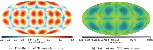
The compactness of the cells is generally lower here due to their rectangular shape, and the distribution is less uniform (Figure 2b) compared to the H3 DGGS hexagonal tessellation. The lowest compactness values were found closer to vertices of the cube, and the highest compactness values are in the central parts of the faces.

3.1.3. OpenEAGGR ISEA4T

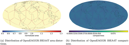
Figure 3(a) illustrates a uniform distribution of area values provided by the ISEA projection. The OpenEAGGR implementation or artifacts of the cells generation and area calculation processes may be the cause of some of the observable outliers. Lower area values are the vertices of the icosahedron, and higher values are near the edges. The significantly lower compactness values compared to other DGGSs (Figure 3b) are the result of the triangular shape of the cells of the tessellation. The irregular pattern for compactness values is common for ISEA projections, as the shapes are distorted to preserve area. On each face of the icosahedron, the shape distortion is distributed along the lines connecting the face’s centroid with its vertices.

Figure 3. Global map of normalized area and compactness values for OpenEAGGR DGGS cells.

3.1.4. rHEALPix

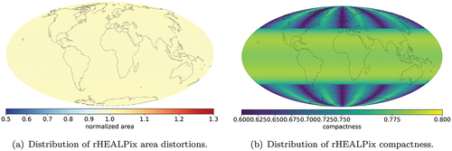
Although the base solid of the rHEALPix DGGS is a cube, the use of 4 different tessellation shape and the equal area rHEALPix projection allow it to achieve almost uniform area values (Figure 4a). There are only minor (less than 0.01 of normalized area units) differences present between mid and high latitudes. The compactness values are distributed based on the different cell shapes – the highest values are for squares in the midlatitudes, the lowest are for triangular cells in the higher latitudes (Figure 4b).

Figure 4. Global map of normalized area and compactness values for rHEALPix cells.

3.1.5. DGGRID

DGGRID can be used to generate various DGGSs with an icosahedron as the base solid, the flexibility to select other essential parameters, and the flexibility to use a different tessellation shape, aperture, projection, and orientation. Area and compactness properties are shown for comparison of six DGGS types, three tessellation shape, and across two projections. DGGRID provides several more variations, including aperture 3 and 4 hexagonal tessellations. We did not include those because they are not congruent. Although, aperture 7 hexagonal DGGS are also not absolutely congruent, indexing systems can enable their reliable and idempotent parent-child-hierarchy. All ISEA-based DGGSs have very low standard deviations for the normalized area metric.

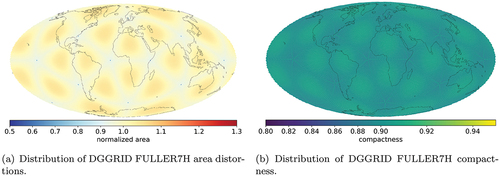
3.1.6. DGGRID ISEA7H and FULLER7H

The aperture 7 hexagonal DGGS types ISEA7H (Figure 5a) and FULLER7H are similar to Uber H3, but use the ISEA or Fuller-Gray projections, respectively, instead of the Gnomonic projection which H3 uses. Figure 6a illustrates that the normalized area values distribution pattern for FULLER7H is similar to that of Uber H3, but the range in values is significantly lower and the distribution closer to uniform. Lower area values are concentrated at vertices and edges of the icosahedron faces, where also singular pentagons are located. Higher values are distributed at the central parts of the faces. The outliers with higher values are most likely caused by peculiarities in the Python libraries used for geometry generation for area calculations, and lie at the boundary zones of the faces of the base icosahedron. However, compactness has the same ISEA distortion pattern (Figure 5b) but the distribution of compactness values for FULLER7H (Figure 6b) is more uniform compared to the ISEA variant but still worse than H3 with its Gnomonic projection. Thus, these results support the fact shown in previous studies (White, Kimerling, Sahr, & Song, 1998) that Fuller-Gray projection gives a compromise option in terms of area versus shape preservation between ISEA and Gnomonic projections.

Figure 5. Global map of normalized area and compactness values for DGGRID ISEA7H cells.

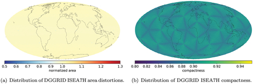
Figure 6. Global map of normalized area and compactness values for DGGRID FULLER7H cells.

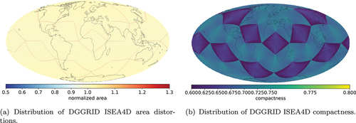
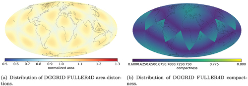
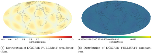
3.1.7. DGGRID ISEA4D and FULLER4D

The ISEA4D and FULLER4D DGGSs use diamonds, also called rhombuses, for tessellation shape. The diamond shape is identical in its properties to a square. Thus, familiar and well-developed indexing and analytical algorithms based on quad-tree can be utilized for this type of DGGS.

Figure 7(a) illustrates the uniform distribution of area values provided by ISEA projection. Still, vertices and edges of the underlying icosahedron tend to be regions of maximal distortions where all outliers are concentrated. The distribution of the compactness values differs from the hexagonal and triangular versions of ISEA-based DGGS (Figure 7a). Absolute compactness values are lower than in hexagonal tessellations but close to squares.

Figure 7. Global map of normalized area and compactness values for DGGRID ISEA4D cells.

Figure 8(a) shows FULLER4D area values have a non-uniform distribution following the same pattern as in ISEA or Gnomonic projections. Maximal values tend to concentrate closer to the centroids of the faces, the minimal values at the edges and vertices of the base icosahedron. The compactness values for FULLER4D (Figure 8b) illustrate a different pattern compared to hexagonal or triangular versions of DGGS with a Fuller-Gray projection.

Figure 8. Global map of normalized area and compactness values for DGGRID FULLER4D cells.

3.1.8. DGGRID ISEA4T and FULLER4T

The ISEA4T and FULLER4T DGGSs use triangles for tessellation shape and are directly comparable to the OpenEAGGR ISEA4T (cf. Figure 3). The triangular tessellation is implemented as a fully congruent aperture 4 DGGS. The ISEA4T configuration provides strong equal area reliability (Figure 9a), except the few pentagons at the vertices of the base polyhedron. Overall, triangles provide the weakest compactness settings in both, the ISEA and Fuller-Gray projection configurations (Figures 9b and 10b)

Figure 9. Global map of normalized area and compactness values for DGGRID ISEA4T cells.

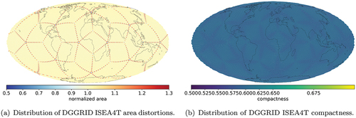
Figure 10. Global map of normalized area and compactness values for DGGRID FULLER4T cells.

3.2. Side-by-side comparison of normalized area and compactness values between DGGSs

The normalized area and compactness values allow comparing fundamental properties for the different DGGSs (Figure 11). The graph illustrates the superiority of rHEALPix and ISEA-based DGGSs for global area preservation. Almost 99.3% of cell areas are close to the mean value in such DGGSs with a few outliers due to either pentagons in hexagonal tessellations or artifacts from the libraries used for the calculations and cells geometry construction. The Fuller-Gray-based DGGSs of DGGRID still have very reliable area consistency, with much better values than H3 or S2.

Figure 11. Summary boxplots of normalized area and compactness values for the cells of the tested DGGSs.

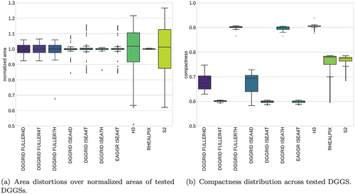
Figure 11(b) shows that all hexagonal DGGSs have the best compactness with values around 0.9 as expected. DGGSs with triangular tessellation are the least compact, with values around 0.6. The Gnomonic projection of the H3 library provides the highest compactness among other hexagonal versions, and with the smallest standard deviation. The S2 and rHEALPix square-based DGGSs have surprisingly high compactness values compared to the aperture 4 diamond-based DGGSs of DGGRID. The large skew for rHEALPix compactness corresponds to the triangles and quads of the “dart” and “skew” cells in high latitudes. The outliers in the DGGRID and OpenEAGGR systems (all have icosahedron as the base solid) consistently stem from the regions where the faces of the icosahedron join. In hexagonal systems, these singularities are caused by the required pentagons (ISEA7H and FULLER7H). In triangular configurations, the outliers are also located in the same regions instead of the pentagons. In H3 (also an aperture 7 hexagonal DGGS) the Gnomonic projection preserves area the least and, thus, the effect is even stronger visible.

4. Discussion

The growing frequency of publications related to Discrete Global Grids Systems (DGGS) and their usage for spatial data management at global scale indicates surging interest in the topic. Outside of the scientific community, businesses and the wider public are also adopting DGGS-based solutions, in particular Uber H3 and Google S2. One increasingly common architecture concept for large-scale spatial analytics are data cubes. Data cubes are already a well-established paradigm for managing remote sensing data in the Earth Observation domain. There are three crucial requirements for a DGGS implementation for this purpose. The first would be equal area preservation for cells throughout resolution levels on a global scale. The second most important would be a congruent hierarchical indexing and addressing system for fast querying across datasets and layers. Thirdly, there is a need for a set of convenient methods to work with the underlying grid structure to support integration in GIS workflows to ingest raster or vector data, transform it to a common resolution, store, analyze and visualize.

We addressed these points by exploring the open-source DGGS implementations from the perspective of their most important geometric properties, equal-area preservation and compactness. The knowledge can be applied subsequently to choose a DGGS for use-cases that require either preference on areal or shape-preserving properties. Secondly, we selected only practical hierarchical and congruent DGGSs for the analysis. Thirdly, we implemented all our analysis steps in Python, aiming to reduce entry barrier for DGGS-based analyses with the Pangeo integrated ecosystem with the parallel processing library Dask and Jupyter notebooks to promote open, reproducible, and scalable geoscience workflows.

Among the explored libraries Uber H3 provides the most convenient and rich programming interface. However, our study showed that the projection method used to construct H3 DGGS does not provide equal-area cells throughout global coverage. This suggests not to use the H3 library for environmental spatial statistics involving area calculations on a regional or global scale. Bousquin (2021) used it for characterizing coastal environments and stated that the availability and ease of use of functionality for cell addressing and neighborhood traversing in H3 supported the analysis, in comparison to the DGGRID approach (Bousquin, 2021). Therefore, the H3 library might serve as a good example of a DGGS’s potential when a particular implementation is widely accessible and supported.

The second very convenient and well-developed DGGS implementation, Google S2, has even higher area distortions. The S2 advertises itself primarily as a library for fast and efficient computational geometry and spatial indexing on the sphere, and has bindings to several popular programming languages and databases support streamlined data ingestion, storage, and analysis workflows. The rectangular shape of the cells and lower aperture level provides smoother transitions between resolution levels compared to H3, and provides a reliable point indexing system, but less an area-cell-based data discretization engine.

The rHEALPix DGGS library benefits from the underlying equal-area rHEALPix projection and indeed provides the most robust fully congruent hierarchical equal-area cell system across the globe. A challenge for the adoption of the library is that it is currently only implemented in Python. Functions are not yet as ergonomic and fast as in S2 or H3. It would be advantageous to have a high-performance portable base library for rHEALPix to increase adoption. Another potentially crucial issue for some applications is the high aperture 9, which causes large steps in cell size between finer and coarser resolutions. However, there is an increasing interest in applying rHEALPix in research problems (Bowater & Stefanakis, 2018; Bowater & Wachowicz, 2020; Hojati, Robertson, Roberts, & Chaudhuri, 2022; Purss et al., 2019). Furthermore, rHEALPix is the only DGGS in this comparison that explicitly supports arbitrary ellipsoids of revolution as a fully configurable construction parameter, making it the closest approximation to the Earth’s geoid and even applicable to other celestial bodies. In contrast, S2 and many hexagonal/icosahedral DGGSs, including H3, are based on the sphere.

OpenEAGGR implements the ISEA projection for a triangular ISEA4T and hexagonal ISEA3H tessellation, both providing equal-area cells across global coverage. The library has a useful set of methods for convenient DGGS manipulations and conventional spatial data input and output. The fully congruent triangular cells provide high equal-area guarantees but low compactness. However, only the ISEA4T version of OpenEAGGR is fully functional. For ISEA3H, OpenEAGGR allows to construct cells and convert to/from geographic coordinates. However, the library does not implement a hierarchical traversing index, and therefore it is not possible to get child cells unambiguously using the provided methods.

DGGRID is an excellent tool for constructing various DGGSs with desired tessellation shapes using the ISEA projection for area preservation or Fuller-Gray, if shape preservation is desired. The tool can be used for exploration purposes to investigate properties of different DGGSs and to pre-generate grids for subsequent ingestion or binning of point data. Unfortunately, DGGRID only allows to construct a single resolution grid at a time and fill it with data. There are currently no functions for interactive cell addressing, neighborhood, or grid traversal. However, libraries in R and Python have been developed, which allow DGGRID to be used in scientific and data engineering workflows (Barnes, 2018; Correndo, 2019; Kmoch, 2020). In terms of geometric properties, general accessibility, and thus overall potential for further development, the DGGRID software is an important pillar in bridging DGGS and GIS for spatial statistics (Rawson, Sabeur, & Brito, 2021; Robertson, Chaudhuri, Hojati, & Roberts, 2020).

DGGSs have great potential to form a solid basis for a new spatial data analytics paradigm. Unique cell indexes unambiguously encode the exact location throughout different platforms and technologies. This opens a plethora of ’geometry-free’ spatial data manipulations. Due to the uniqueness and recognition of a DGGS cell identifier, it is possible to minimize the size of the transferred data significantly. A DGGS-based data table can be easily partitioned for distributed calculations or storage of significantly larger datasets on a Big Data scales not possible for classic spatial R-tree-based indices. With a DGGS as a basis for a data cube, it is possible to easily combine data from different sources, with different source resolution and data formats, and it would remove the current data cube limitation of being restricted to the extent of a single projected coordinate reference system.

5. Conclusion and outlook

In this study, the open-source DGGS implementations H3, S2, OpenEAGGR, rHEALPix and DGGRID were investigated as alternative spatial data reference and indexing systems. They were examined for two important geometric properties – equal-area preservation and compactness. H3 and S2 have the largest variation in surface area of their DGGS cells and should not be used for a data cube implementation for managing environmental data and spatial statistics where equal area cells are required. rHEALPix and ISEA-based DGGSs, like DGGRID’s ISEA7H, ISEA4T, and ISEA4D are the most reliable in preserving the area across the whole globe. For compactness, hexagonal DGGSs have undeniable advantages, including unambiguous neighborhood relationships and better visual data representation. It could be very useful to have an H3-like implementation of an ISEA7H DGGS, an equal area hexagonal DGGS with the usability of H3. This could also reduce the burden of the high aperture and different tessellation shapes of rHEALPix.

Another remaining bottleneck is data conversion, i.e. discretizing and loading data into a DGGS-based data structure. This quantization step depends on the spatial sampling techniques and chosen resolutions, because there are no well-tested standard methods to transform raster or vector data into a DGGS-based data cube and preserve information efficiently. Furthermore, the next logical step is to extend available DGGS implementations into the third dimension, aka voxel based DGGS configurations – this could be defined as the roadmap to global volume-based data cubes.

Finally, for the adoption and popularization of DGGS to a wider audience, it is necessary to improve the implementations of DGGS-based tools in desktop and web-based GIS software. Here, H3 and S2 are preferable. Our call to action is to invest in the integration of existing open-source DGGS implementations with prominent geospatial analytics software ecosystems such as Pangeo (Pangeo project, 2022).

Acknowledgement(s)

The authors would like to thank the reviewers and the editor for the constructive feedback and the insightful comments on the manuscript which greatly improved the work.

Disclosure statement

No potential conflict of interest was reported by the author(s).

Data availability statement

The data that support the findings of this study are openly available on “Zenodo” at https://doi.org/10.1080/20964471.2022.2094926, reference number 6634479 Version v1.0.2.

Supplementary data

Supplemental data for this article can be accessed online at https://doi.org/10.1080/20964471.2022.2094926.

Additional information

Funding

This research has been supported by the Marie Skłodowska-Curie Actions individual fellowship under the Horizon 2020 Programme grant agreement number 795625, grant number MOBERC34 of the Estonian Research Council (ETAG), and the NUTIKAS programme of the Archimedes foundation. The authors are also thankful for technical support from the High Performance Computing Center of the University of Tartu.

Notes on contributors

Alexander Kmoch

Alexander Kmoch, PhD, is a Research Fellow in Geoinformatics at the University of Tartu. He works on Distributed Spatial Systems and has many years of international experience in geospatial data management and web- and cloud-based geoprocessing with a particular focus on land use, soils, hydrology, and water quality. His interests include OGC standards and web-services for location-based data sharing, modeling workflows, machine learning, and interactive geo-visualisation.

References

- Alderson, T., Purss, M., Du, X., Mahdavi-Amiri, A., & Samavati, F. (2020). Digital earth platforms. In H. Guo, M. F. Goodchild, & A. Annoni (Eds.), Manual of Digital Earth (1st ed., (pp. 25–55). Singapore: Springer.
- Barnes, R. (2018). Dggridr: Discrete global grids for r v2.0.3. [Software]. Zenodo. doi:10.5281/zenodo.1322866.
- Bauer-Marschallinger, B., Sabel, D., & Wagner, W. (2014). Optimisation of global grids for high-resolution remote sensing data. Computers & Geosciences, 72, 84–93. doi:10.1016/j.cageo.2014.07.005
- Baumann, P. (2021). A general conceptual framework for multi-dimensional spatio-temporal data sets. Environmental Modelling & Software, 143, 105096. doi:10.1016/j.envsoft.2021.105096
- Bondaruk, B., Roberts, S. A., & Robertson, C. (2020, March). Assessing the state of the art in discrete global grid systems: OGC criteria and present functionality. Geomatica, 74(1), 9–30. doi:10.1139/geomat-2019-0015
- Bousquin, J. (2021, December). Discrete global grid systems as scalable geospatial frameworks for characterizing coastal environments. Environmental Modelling & Software, 146, 105–210. doi:10.1016/j.envsoft.2021.105210
- Bowater, D., & Stefanakis, E. (2018). The rHealpix discrete global grid system: Considerations for Canada. Geomatica, 72(1), 27–37. doi:10.1139/geomat-2018-0008
- Bowater, D., & Wachowicz, M. (2020, May). Modelling offset regions around static and mobile locations on a Discrete Global Grid system: An IoT case study. ISPRS International Journal of Geo-Information, 9(5), 335. doi:10.3390/ijgi9050335
- Breunig, M., Bradley, P. E., Jahn, M., Kuper, P., Mazroob, N., Rösch, N., Jadidi, M. … Jadidi, M. (2020, February). Geospatial data management research: Progress and future directions. ISPRS International Journal of Geo-Information, 9(2), 95. doi:10.3390/ijgi9020095
- Bush, I. (2017). OpenEAGGR - Open Equal Area Global GRid. [Software]. Bristol: RiskAware Ltd. Retrieved from https://github.com/riskawaretd/openaggr
- Chaudhuri, C., Gray, A., & Robertson, C. (2021, June). InundatEd-V1.0: A height above nearest drainage (HAND)-based flood risk modeling system using a discrete global grid system. Geoscientific Model Development, 14(6), 3295–3315. doi:10.5194/gmd-14-3295-2021
- Correndo, G. (2019). dggridpy: A python binding to the DGGRID library. [Software]. GitHub. Retrieved from https://github.com/correndo/dggridpy
- de Sousa, L. M. (2018). Remaining gaps in open source software for Big Spatial Data. Peer J Preprints, 6: e27215v2. https://doi.org/10.7287/peerj.preprints.27215v2.
- de Sousa, Poggio, L., Luis, M., Poggio, L., & Kempen, B. (2019, August). Comparison of FOSS4G supported equal-area projections using discrete distortion indicatrices. ISPRS International Journal of Geo-Information, 8(8), 351. doi:10.3390/ijgi8080351
- Dutton, G. (1989, April). Planetary modelling via hierarchical tessellation. International conference on computer-assisted cartography (auto-carto 9) (pp. 462–471). Baltimore.
- Gibb, R., Raichev, A., & Speth, M. (2016). The rHEALPix DGGS preprint. Retrieved from https://raichev.net/files/rhealpixdggspreprint.pdf
- Giuliani, G., Chatenoux, B., De Bono, A., Rodila, D., Richard, J.-P., Allenbach, K., Peduzzi, P. … Peduzzi, P. (2017, December). Building an earth observations data cube: Lessons learned from the Swiss Data Cube (SDC) on generating Analysis Ready Data (ARD). Big Earth Data, 1(1–2), 100–117. doi:10.1080/20964471.2017.1398903
- Goodchild, M. F., & Shiren, Y. (1992). A hierarchical spatial data structure for global geographic information systems. CVGIP: Graphical Models and Image Processing, 54(1), 31–44.
- Goodchild, M. F. (2018, January). Reimagining the history of GIS. Annals of GIS, 24(1), 1–8. doi:10.1080/19475683.2018.1424737
- Gorski, K. M., Hivon, E., & Wandelt, B. D. 1998. Analysis issues for large cmb data sets. arXiv. eprint: astro-ph/9812350.
- Gray, R. W. (1995). Exact transformation equations for Fuller’s world map. Cartographica, 32(3), 17–25. doi:10.3138/1677-3273-Q862-1885
- Gregory, M. J., Kimerling, A. J., White, D., & Sahr, K. (2008, May). A comparison of intercell metrics on discrete global grid systems. Computers, Environment and Urban Systems, 32(3), 188–203. doi:10.1016/j.compenvurbsys.2007.11.003
- Guo, H. (2017). Big Earth data: A new frontier in Earth and information sciences. Big Earth Data, 1(1–2), 4–20. doi:10.1080/20964471.2017.1403062
- Hamilton, C. H., & Rau-Chaplin, A. (2008). Compact Hilbert indices: Space-filling curves for domains with unequal side lengths. Information Processing Letters, 105(5), 155–163. doi:10.1016/j.ipl.2007.08.034
- Hilbert, D. (1891). Ueber die stetige Abbildung einer Linie auf ein Flaechenstueck. Mathematische Annalen, 38(3), 459–460. ( (in German)). doi:10.1007/BF01199431
- Hojati, M. (2019). Pydggrid: Python wrapper for dggrid v0.0.1. [Software]. Zenodo. doi:10.5281/zenodo.3228406
- Hojati, M., Robertson, C., Roberts, S., & Chaudhuri, C. (2022, January). Giscience research challenges for realizing discrete global grid systems as a Digital Earth. Big Earth Data, 1–22. doi:10.1080/20964471.2021.2012912
- Jendryke, M., & McClure, S. C. (2019, October). Mapping crime – Hate crimes and hate groups in the USA: A spatial analysis with gridded data. Applied Geography, 111, 102072. doi:10.1016/j.apgeog.2019.102072
- Jordahl, K., & Contributors, G. (2021). Geopandas: Python tools for geographic data. [Software]. Zenodo. Retrieved from doi:10.5281/zenodo.4569086
- Kimerling, J. A., Sahr, K., White, D., & Song, L. (1999). Comparing Geometrical Properties of Global Grids. Cartography and Geographic Information Science, 26(4), 271–288. doi:10.1559/152304099782294186
- Kmoch, A. (2020). Dggrid4py: A set of python modules for creating and manipulating Discrete Global Grids with DGGRID. v0.2.3. [Software]. Zenodo. doi:10.5281/zenodo.5873330
- Kmoch, A., & Vasilyev, I. (2022a). Code supplement for open-source dggs cell geometry comparisons. [Software]. Zenodo. doi:10.5281/zenodo.5905935
- Kmoch, A., & Vasilyev, I. (2022b). Data supplement for open-source dggs cell geometry comparisons. [Dataset]. Zenodo. doi:10.5281/zenodo.6634479
- Lei, K., Qi, D., & Tian, X. (2020, January). A new coordinate system for constructing spherical grid systems. Applied Sciences, 10(2), 655. doi:10.3390/app10020655
- Lewis, A., Oliver, S., Lymburner, L., Evans, B., Wyborn, L., Mueller, N., Wang, L. W. … Wang, L. W. (2017). The Australian Geoscience Data Cube — Foundations and lessons learned. Remote Sensing of Environment, 202, 276–292. doi:10.1016/j.rse.2017.03.015
- Li, W., Goodchild, M. F., & Church, R. (2013, June). An efficient measure of compactness for two-dimensional shapes and its application in regionalization problems. International Journal of Geographical Information Science, 27(6), 1227–1250. doi:10.1080/13658816.2012.752093
- Li, M., & Stefanakis, E. (2020, December). Geospatial operations of discrete global grid systems - A comparison with traditional GIS. Journal of Geovisualization and Spatial Analysis, 4(2), 26. doi:10.1007/s41651-020-00066-3
- Li, Z., Gui, Z., Hofer, B., Li, Y., Scheider, S., & Shekhar, S. (2020). Geospatial information processing technologies. In H. Guo, M. F. Goodchild, & A. Annoni (Eds.), Manual of digital earth (1st ed., pp. 191–227). Singapore: Springer Singapore.
- Liao, C., Tesfa, T., Duan, Z., & Leung, R. (2020, June). Watershed delineation on a hexagonal mesh grid. Environmental Modelling & Software, 128, 104702. doi:10.1016/j.envsoft.2020.104702
- Lin, B., Zhou, L., Xu, D., Zhu, A.-X., & Lu, G. (2018, April). A discrete global grid system for earth system modeling. International Journal of Geographical Information Science, 32(4), 711–737. doi:10.1080/13658816.2017.1391389
- Mahdavi-Amiri, A., Harrison, E., & Samavati, F. (2014, September). Hexagonal connectivity maps for Digital Earth. International Journal of Digital Earth, 8(9), 750–769. doi:10.1080/17538947.2014.927597
- Mahdavi-Amiri, A., Alderson, T., & Samavati, F. (2015, December). A survey of Digital Earth. Computers & Graphics, 53, 95–117. doi:10.1016/j.cag.2015.08.005
- Montibeller, B., Kmoch, A., Virro, H., Mander, Ü., & Uuemaa, E. (2020, December). Increasing fragmentation of forest cover in Brazil’s Legal Amazon from 2001 to 2017. Scientific Reports, 10(1), 5803. doi:10.1038/s41598-020-62591-x
- Open Geospatial Consortium. (2017). Topic 21: Discrete global grid systems abstract specification. The Open Geospatial Consortium (OGC). Retrieved from https://portal.opengeospatial.org/files/15-104r5.pdf
- Osserman, R. (1978). The isoperimetric inequality. Bulletin of the American Mathematical Society, 84(6), 1182–1238. doi:10.1090/S0002-9904-1978-14553-4
- Pangeo project. (2022). A community platform for Big Data geoscience. Retrieved from https://pangeo.io/
- Purss, M. B. J., Gibb, R., Samavati, F., Peterson, P. R., & Ben, J. (2016, July). The OGC Discrete Global Grid System core standard: A framework for rapid geospatial integration. 2016 IEEE International Geoscience and Remote Sensing Symposium (IGARSS), Beijing, China, July 10-15, 2016, (pp. 3610–3613). IEEE.
- Purss, M. B. J., Peterson, P. R., Strobl, P., Dow, C., Sabeur, Z. A., Gibb, R. G., & Ben, J. (2019, March). Datacubes: A Discrete Global Grid Systems perspective. Cartographica, 54(1), 63–71. doi:10.3138/cart.54.1.2018-0017
- Rawson, A., Sabeur, Z. A., & Brito, M. (2021, September). Intelligent geospatial maritime risk analytics using the Discrete Global Grid System. Big Earth Data, 1–29. doi:10.1080/20964471.2021.1965370
- Robertson, C., Chaudhuri, C., Hojati, M., & Roberts, S. A. (2020, April). An integrated environmental analytics system (IDEAS) based on a DGGS. ISPRS Journal of Photogrammetry and Remote Sensing, 162, 214–228. doi:10.1016/j.isprsjprs.2020.02.009
- Sahr, K. (2008). Location coding on icosahedral aperture 3 hexagon discrete global grids. Computers, Environment and Urban Systems, 32(3), 174–187. doi:10.1016/j.compenvurbsys.2007.11.005
- Sahr, K. (2011). Hexagonal discrete global grid system for geospatial computing. Archives of Photogrammetry, Cartography and Remote Sensing, 22, 363–376.
- Sahr, K. (2019). DGGRID version 7.0. [Software]. Retrieved from https://www.discreteglobalgrids.org/software/
- Seong, J. C., Mulcahy, K. A., & Usery, E. L. (2002). The sinusoidal projection: A new importance in relation to global image data. Professional Geographer, 54(2), 218–225. doi:10.1111/0033-0124.00327
- Snyder, J. P. (1992). An equal-area map projection for polyhedral globes. Cartographica, 29(1), 10–21. doi:10.3138/27H7-8K88-4882-1752
- Uber Technologies Inc. (2018). H3: Hexagonal hierarchical geospatial indexing system. [Software]. Retrieved from https://h3geo.org/
- Veach, E., Rosenstock, J., Engle, E., Snedegar, R., Basch, J., & Manshreck, T. (2017). S2 Geometry Library: Computational geometry and spatial indexing on the sphere. [Software]. Retrieved from https://s2geometry.io
- White, D., Kimerling, J. A., Sahr, K., & Song, L. (1998, December). Comparing area and shape distortion on polyhedral-based recursive partitions of the sphere. International Journal of Geographical Information Science, 12(8), 805–827. doi:10.1080/136588198241518
- White, D. (2000). Global grids from recursive diamond subdivisions of the surface of an octahedron or icosahedron. Environmental Monitoring and Assessment, 64(1), 93–103. doi:10.1023/A:1006407023786
- Yao, X., Li, G., Xia, J., Ben, J., Cao, Q., Zhao, L., Zhu, D. … Zhu, D. (2020, January). Enabling the big earth observation data via cloud computing and DGGS: Opportunities and challenges. Remote Sensing, 12, 1.