Assessing suspended sediment fluxes with acoustic Doppler current profilers: case study from large rivers in Russia

ABSTRACT

Surrogate measures are becoming increasingly used to measure suspended sediment flux, but only few particular computer techniques of data processing are recently developed. This study demonstrates capabilities of acoustic Doppler current profilers (ADCPs) to infer information regarding suspended-sand concentrations in river systems and calculate suspended sediment flux via big data analytics which includes process of analyzing and data mining of measurements based on ADCP signal backscatter intensity data. We present here specific codes done by R language using RStudio software with open-source tidyverse and plotly packages aimed to generate tables containing data of suspended load for cells, verticals and whole cross-section based on backscattering values from 600 kH Teledyne RDInstruments RioGrande WorkHorse ADCP unit, as well perform estimates of morphometric, suspended sediment concentration (SSC) and velocity characteristics of the flow. The developed tools enabled to process large data array consisting of over 56,526,480 geo-referenced values of river depth, streamflow velocity, and backscatter intensity for each river cross-section measured at six case study sites in Russia.

KEYWORDS:

• Big data
• ADCP
• backscatter intensity
• sediment transport

1. Introduction

Sediments are an integral and dynamic part of aquatic systems and play a major role in the hydrological, geomorphological, and ecological functioning of river basins (Chalov, Golosov, & Tsyplenkov et al., 2017; Collins & Walling, 2007; Kemp, Sear, & Collins et al., 2011; Walling, 2006). It is a conglomerate of organic and inorganic materials that can be soil particles, mineral matter, decomposing organic substances, inorganic biogenic material which can be transported as a suspended (floating in the water column) or bed-load (carried in near-bed layer). Most mineral sediments come from bed erosion and soil and bedrock weathering. Organic sediments are typically detritus and decomposing materials such as algae and further are related to suspended sediments. River sediments carry tremendous quantities of chemicals including the most challenging for the environment such as heavy metals, nutrients, PAH (Horowitz, 1985; Townsend, Uhlmann, & Matthaei, 2008).

Due to the comprehensive nature of origin, studies on sediment transport remain one of the most complicated segments of land surface hydrology. Traditional measurement methods are often used to estimate suspended-sediment transport rates based on the deployment of appropriate instantaneous physical suspended sediment samplers (e.g Edwards and Glysson (1999), and Davis (2005)) and, if sampling from a boat, holding the boat stationary for water column sediment sampling (Diplas, Kuhnle, & Gray et al., 2008). Studies on the interaction of flow and sediment transport, quantitative assessment of hydrodynamic sorting of suspended sediment within the depth column are mostly based on laboratory datasets (Julien, 2010); whereas recent field data from the Amazon River (García, 2008), Ganges River (Lupker, France-Lanord, & Lavé et al., 2011), Parana River (Szupiany et al., 2019) significantly extended knowledge on suspended sediment behavior over large rivers cross-sections. Dimensionless Rouse number (Ro) is widely applied to describe the ratio of upward and downward forces acting on the grains in the fluid:

(1) $Ro=\frac{\omega s\hspace{0.17em}}{\beta k{V}_{\ast }}$(1)

where k is von Karman’s constant (0.41), ωs is settling velocity (m/s) of the sediments, which is a function of grain size, shape and density, $V_{\ast }$ is bed shear velocity, and $\beta$ the ratio of sediment and water momentum diffusion coefficients, generally assumed to be 1. Within small- and medium-sized rivers conditions lower than the critical Rouse number, Ro* = 2.5 indicates that a sediment particle begins to contribute to the suspended load (Lynds, Mohrig, Hajek, & Heller, 2014). Whereas higher values indicate that a sediment particle is most likely transported as part of the bed load. Rouse number explains the theoretical Rouse profile of sediment distribution:

(2) $\frac{S}{S_a}=\hspace{0.17em}{\left(\frac{h-z}{z}\frac{a}{h-a}\right)}^{Ro}$(2)

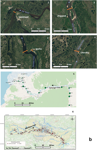
S – suspended sediment concentration (SSC), S_a – near bottom suspended sediment concentration, h – river depth, z – normalized depth at point, Ro – Rouse number, a – near-bottom layer at distance from the bottom a = 2×D₅₀, where D₅₀ – mean bottom sediment diameter. As a milestone in the history of sediment transport, the Rouse formula (1) has been widely used for decades (Chalov, Moreido, & Sharapova et al., 2020; Graf & Cellino, 2002; Zheng, Li, Feng, & Lu, 2013). However, limitations of this theory were widely known (Julien, 2010). Nevertheless, all these studies rely on limited empirical data and validation was nearly impossible. The empirical data to establish criteria of each mode are very limited (Bouchez, Métivier, & Lupker et al., 2011; Lupker, France-Lanord, & Lavé et al., 2011).

This and other aspects of surface water sediment transport were recently significantly improved due to application of sediment concentration surrogate technologies measurements which are based on optical, laser, and acoustic principles (Gray & Gartner, 2009; Pomázi & Baranya, 2020). Acoustic technologies, based on commercial acoustic Doppler current profilers (ADCPs), have been recognized as potential tools for the quantification of sediment transport in natural streams using the echo intensity levels as a measure of acoustic backscattering strength. The acoustic methods are based on assessing the velocity within a unit volume of water by measuring the Doppler shift of the frequency of the ultrasonic signal emitted by the ADCP instrument and reflected from the suspended matter within this volume. Common operation frequencies for ADCPs cover the range between 300 and 3,000 kHz. To measure water discharge, the ADCP unit is mounted on the moving boat or other vessel and transmits acoustic signals into the water column towards the river bottom. The echoes of the signal reflected from small particles of mineral and organic matter are referred to as backscatter intensity. The latter is subsequently attributed to different depths within the measured range to the bottom yielding the backscatter and velocity vertical profile. Commonly, the ADCP units have 1 to 9 ultrasonic emitters which operate at a various frequency range which allows for simultaneous quality control of the received signal. Furthermore, the ADCP units are additionally equipped with echosounders and GPS receivers which enable measurements within the local (by tracking the river bottom) or global coordinate systems. This allows for accurate water velocity measurements as the boat speed is subtracted from the stream flow velocity. As the boat moves across the river from one bank to the other the vertical profiles are seamlessly combined to form the cross-sectional velocity map which allows for stream flow discharge calculation (Mueller & Wagner, 2009).

Results of pioneer applications of an acoustic techniques for suspended sediment concentration (SSC) measurements identified outstanding potential of this approach (Deines, 1999; Holdaway, Thorne, Flatt, Jones, & Prandle, 1999; Mullison, 2017; Thorne, Vincent, Hardcastle, Rehman, & Pearson, 1991; Wang, Chu, Lee, Han, & Oh, 2005; Wang, Gao, & Li, 2000; Wang, Pan, & Wang, 2006). Whereas the uncertainties of these measurements due to impact of physical properties of the solids on sound scattering in water were discussed (Hanes, 2012; Moore, Le, Hurther, & Paquier, 2013; Thorne & Hanes, 2002; Thorne & Meral, 2008). Nevertheless, later it was widely used to study large tidal rivers (Wall, Nystrom, & Litten, 2006), river confluences (Hackney et al., 2018; Szupiany et al., 2019 and 2009), sediment propagation during floods (Guerrero & Federico, 2018) and allowed to understand spatial and temporal distribution of SSC faster and cheaper compared to traditional methods (Latosinski, Szupiany, & García et al., 2014; Topping & Wright, 2016). As of today, there are a lot of regional studies, where acoustic methodology applied with some empirical additions for rivers, estuaries over the world. The case studies were devoted for the delta of Mahakam River, India (Sassi, Hoitink, & Vermeulen, 2012), big rivers such as Fraser River, Canada (Venditti, Church, Attard, & Haught, 2016), the Danube (Pomázi & Baranya, 2020), the Rona (Sakho et al., 2019) and small rivers of the Anatolian Peninsula (Elçi, Aydın, & Work, 2009). There are a lot of studies about applying ADCPs for freshwater SSC monitoring (Aleixo, Guerrero, Nones, & Ruther, 2020; Moore, Le, Hurther, & Paquier, 2013). Significant part of studies provides the comparisons of acoustic and other indirect methods such as laser diffraction and nephelometry (Agrawal & Hanes, 2015; Pomázi & Baranya, 2020).

The ADCP-discharge measurement provides large amount of backscatter and velocity data that is received with every measured cross-sectional profile and thus is applicable for suspended sediment concentrations analyses. The use of down-looking ADCPs to estimate SSC has been investigated by many researchers (Boldt et al., 2012; Boldt, 2015; Dominguez Ruben et al., 2020; Gartner, 2004; Guerrero, Szupiany, & Latosinski, 2013; Latosinski, Szupiany, & García et al., 2014; Moore, Le, Hurther, & Paquier, 2013; Mullison, 2017; Szupiany et al., 2016, 2019; Wall, Nystrom, & Litten, 2006; Wood, Szupiany, Boldt, Straub, & Domanski, 2019). Several software tools have been developed (STA described in Boldt et al. (2012); ASET used in Szupiany et al. (2016)); and commercial software such as Aquavision’s ViSea to process ADCP data for use in estimating SSC. Nevertheless, the cited software is mostly related to calculating suspended sediment flux, whereas do not allow to process particular data of sediment concentrations within river cross-section in combination with morphometric and hydraulic information. At the same time the implication of programming and design tools that are nowadays realized in packages for modern high-level programming languages such as R, Python, etc., represent reliable background for developing such methodology which can improve understanding of sediment behavior and related hydrological phenomena.

This paper aims to apply acoustic inversion techniques using commercially available, down-looking acoustic Doppler current profilers (ADCPs) to quantify suspended sediments fluxes in river channels. In particular, we aim (1) to develop an integrated freely available open-source tools of ADCP big data analytics (process of analyzing and data mining of measurements), (2) to demonstrate its applications for understanding sediment concentration of particulate matter distribution over cross-sections, (3) considering accuracy of ADCP data, to estimate sediment concentrations, attempt to improve the assessment of the suspended sediment flux and related phenomena of suspended to bed load partitioning. In the paper, we describe 6 case studies that enable testing the big data analytics over various conditions. The methodology was tested over the largest Arctic rivers of Russia (namely the Ob, Yenisey, Lena and Kolyma rivers, case studies 1–4), at the Selenga River which is the largest tributary of the Baikal Lake (case study 5) and along the Moskva River and its tributaries draining the largest megacity of Russia – the Moscow city (case study 6).

2. Data collection and methods

Both large and small rivers were encompassed during the ADCP methodology application. The variability of conditions from the case studies allowed for testing the proposed methodology robustness. The collected datasets (freely available from Zenodo, Chalov, Moreido, and Ivanov et al. (2022)) were used here to develop the proposed tools for ADCP application in sediment and particulate chemicals transport research.

Case studies 1–4 (Figure 1(a)) comprise the four largest Arctic Siberian rivers which were studied under the ArcticFLUX project in 2018–2021 (Vihma, Uotila, & Sandven et al., 2019) and included continuous ADCP measurements along with a sampling of the dissolved and particulate organic matter, nutrients, and metals fluxes based on unprecedentedly dense river cross-section inventory multiple times per year. Here the measurements were done at constant cross-section at each river located upper from the impact of recipient seas (tides, surges) near the cities of Salekhard (Ob River), Igarka (Yenisey River), Zhigansk (Lena River) and Cherskiy (Kolyma River).

Figure 1. Case studies of ADCP applications. a) General sketch map: blue circles – Arctic rivers (1 – Ob, 2 – Yenisey, 3 – Lena, 4 – Kolyma), yellow circle − 5 – Selenga River; red circle − 6 – Moscow River and its’ tributaries; b) local stream reaches maps: location of the cross-sections for the case studies 1–4 – orange lines; for the case study 5 – green dots; for the case study 6 – red dots.

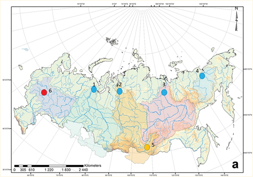
Figure 1. (continued).

Case study 5 is the Selenga River, which originates in Mongolia, and contributes about 50% of the total inflow and 82% of sediment load into the Baikal Lake. The study here was based on detailed ADCP measurements over 20 transects (named S1 … S26, Figure 1b) in the lower 200 km of the river course.

Case study 6 is the Moskva River which is a relatively small stream in Central Russia influenced by dam regulation, water transfer projects and tremendous wastewaters loads from the Moscow city reaching population of 15 mln (Bityukova & Koldobskaya, 2018; Kirillov, Makhrova, & Nefedova, 2019). The urban sewage from Moscow City, which contributes to half of the total water flow downstream of the city, is rich in nutrients and organic matter and therefore plays a large part in the Moskva River organic pollution (Tereshina, Erina, & Sokolov et al., 2020). ADCP measurements and water quality sampling network at 38 points have been established since 2019 along the Moskva River (named M1, M2) and 17 tributaries (named T01, T02) (Table 1, Figure 1).

Table 1. Summary of hydraulic and sediment measurements of the studied rivers used in this study.

River	Period of measurement	Water runoff, m^3/s	Max depth, m	River width,m	Mean depth, m	Mean water velocity, m^2/s	Measured suspended load (R), kg/s	Mean Rouse number	Suspended sediments mean grain size, mm	Calculate bed load (G), kg/s (5)-(7)	R/(R+G)	Mean water slope, m/km
Yenisey	04.06–15.05.2019	>90,000	30–65	393–1,823	16–28	0.46–1.82	318–9,275	0.13–0.2	0.06–0.16	571–608	0.55–0.85	1.96
Kolyma	27.06–15.07.2019; 30.06.2020–10.07.2020	8,164–8,805	12–16	2,801–3,091	6–7	0.48–1	490–556	0.24–0.3	0.034	1561	0.25	0.5
Ob	21.09–24.09.2018; 27.06–05.07.2019	11,964–34,022	21–28	1,720–2,257	10–13	0.58–1.07	1,478–2,736	0.21–0.49	0.09–0.22	261–1,865	0.85–0.93	0.92–1.93
Selenga	27.07.2018–31.07.2018	274–2,675	2–10	70–399	2–3	0.54–2	59–564	0.81–2.76	0.01–0.02	1,362–22,980	0.02–0.11	2.60
Lena	05.05.2019–15.06.2019	8,000–18,000	6–8	1,200–2,200	5–8	0.6–0.8	80–550	0.1–0.4	0.1–0.12	–	–	0.5
Moskva	05.07.2019–30.08.2019	2–18	2–3	10–120	1–2	0.5–0.7	54–230	0.8–1	0.01–0.06	5.32–20	0.8–0.9	–

For each of the case study rivers (Table 1) water discharge Q and suspended load data collection were carried out by discharge measurements using an Acoustic Doppler Current Profiler (ADCP) unit. We used the Teledyne RDInstruments RioGrande WorkHorse ADCP unit with working frequency of 600 kHz mounted on a moving boat. This ADCP system is a downward-looking profiler that broadcasts forward, aft, right- and left-lateral acoustic signals, each angled approximately 20° from the vertical transducer (called a Janus configuration Hauer and Lamberti (2017)). The velocities V and backscatter intensities BI are measured at each depth which can be further used to count flow velocity and echo intensity distributions over a cross-section. The collected data is stored in binary format, which can be natively exported to ASCII format.

For each cross-section three samples (surface, middle layer and near bottom) per three verticals distributed along the transect were obtained. In total, nine samples were taken during a single ADCP measurement. Water samples were pumped out with a filterless submersible 12 V pump from three layers (top, midsection and near-bottom) to account for the vertical distribution of the suspended sediment. Pumping was done with relatively low pressure and speed (approximately 1 liter per minute) which provides relatively unchanged linear velocity (isokinetic sampling). For each sample in a depth profile, the boat was repositioned at its original location, and sampling was performed while drifting at the river water velocity. The depth and width were further marked at the ADCP profile, the point indicated correspondence between measured BI from ADCP and sampled SSC. We used the raw BI values from the ADCP and no backscatter correction was applied (see Szupiany et al. (2019) for BI correction procedure discussion).

The water samples were then filtered for suspended material through a pre-weighted 0.45-μm membrane filter to determine suspended sediment concentration by gravimetric method. The suspended sediment grain size was measured with a Fritsch Analysette 22 NanoTec Laser particle sizer (FRITSCH GmbH, Industriestrasse 8.55743 Idar-Oberstein, Germany). All grain sizes were classified into three categories: clay (grain sizes d <5 μm), silt (d = 5–50 μm), and sand (>50 μm). Based on these results, all rivers were classified as single-modal or bi-modal suspended sediment distributions according to existence 1 or 2 maxima in grain size classes distribution. To calibrate relationship between backscatter and suspended sediment concentration we used power-law least-squares fitting between the raw backscatter values BI and the measured suspended sediment concentration SSC (see additionally in Efimov, Chalov, and Efimova et al. (2019)) for the specific rivers and hydrological seasons. For this purpose, only profiles with sufficient amount of simultaneous SSC gravimetric and ADCP-based BI measurements carried out under constant discharge conditions were considered.

Since we used the raw uncorrected BI values, we constructed separate formulas for each of the case studies.

For the Ob River, we used 27 SSC measurements carried out on 17 and 21 September 2018 and 4 July 2019 (n = 27, 9 samples per measurement) to calibrate SSC=f(BI) relationship (R² = 0.28):

(3) $SSC=\hspace{0.17em}9.16{\mathrm{e}}^{0.02BI}$(3)

Here the low R² is explained by contrasting conditions under field measurement used for the relationship. For the Lena River the SSC=f(BI) relationship was done based on 18 measurements carried out on 08 and 16 June 2019 (n = 18), which lead to the following relationship (R² = 0.57):

(4) $SSC=\hspace{0.17em}0.59{\mathrm{e}}^{0.382BI}$(4)

For the Kolyma River the R² values were equal to 0.31 based on 27 SSC measurement carried out simultaneously with the ADCP profiling on 26 July, 7 August and 16 August 2019:

(5) $SSC=\hspace{0.17em}0.37{\mathrm{e}}^{0.06BI}$(5)

For the Selenga River the measurements were carried out between 27 July and 1 August, 2018 (see additionally in Chalov, Liu, and Chalov et al. (2018)) on an extensive river reach. Based on three samples per ADCP profile, the following fits were obtained (n = 29, R² = 0.42):

(6) $SSC=\hspace{0.17em}0.007{\mathrm{e}}^{0.12BI}$(6)

Finally, for the Moskva River the relationship was based on the two measurements carried out at downstream section M38 of the studied transect (Figure 1) of ADCP profile (n = 18):

(7) $SSC=\hspace{0.17em}3.2{\mathrm{e}}^{0.014BI}$(7)

The datasets for the Yenisey River did not provide sufficient number of SSC gravimetric measurements to capture significant relationship (n = 9).

The dataset was processed in R language using RStudio software (Rstudio Team, 2019) with open-source tidyverse (Wickham, Averick, & Bryan et al., 2019) and plotly packages (Sievert, 2020). The tidyverse package is a state-of-the-art collection of R packages designed for table data manipulation, processing, filtering and analysis. This tool was initially applied to eliminate errors and flaws in the dataset of vertical suspended sediment concentration profiles for each measured river cross-section. The plotly package is the open-source graphical package that allows creation of multiple types of interactive figures (see Supplementary 1). The full code can be accesses from https://sediment.ru/data/R-adcp_v01.zip. The full code consists of three parts with different functionss).

Code 1 is used to convert the backscatter intensity (BI) values to SSC (mg/l), fill in gaps in the original ASCII file, including in the near bottom layer using the Rouse number. In particular, this code provides a calculation of bed load by the L.C. van Rijn model (van Rijn, 2007). The output of the code is a series of tables containing data of suspended load for cells, verticals and the whole cross-section.

Code 2 is used to create a database of morphometric, SSC and velocity characteristics of the flow to find their relationship with the Rouse number. This code creates correlogram graphs for visual analysis and correlation tables of linear regression between SSC, predictors and their simple mathematical transformations.

Code 3 searches for the relationship between the Rouse number and morphometric characteristics, as well as between the Rouse number and SSC using machine learning methods. The output of this code is a series of figures of the distribution of the Rouse number of cells, verticals and whole cross-section within its predictors. Also, this code calculates linear regression coefficients with formulas for the dependence of SSC on morphometric and hydraulic characteristics.

ADCP datasets were applied for assessing suspended load flux (Figure 2). For each ADCP cross-section suspended sediment load Q_R was calculated by averaging the SSC over cross-section with ADCP-based water discharge Q:

(8) $Q_{RADCP}=\underset{0}{\overset{B}{\int }}SSC\cdot Q\cdot dB$(8)

Figure 2. Reference transformation illustrated for the Ob River cross-section in Salekhard (measured on 05.07.19): top panel – backscateter intensity; bottom panel – stream velocity.

The processing of flux estimate requires additional operations due to technological limitation of the ADCP which contains blank (unmeasured) areas in near-bottom part of the transect. For this, extrapolation of suspended sediment concentration in the bottom part of the profile SSC was made by Rouse curve and logarithmic velocity curve by Grishanin (Grishanin, 1972) for each vertical separately to account for SSC distribution in the river cross-section

(9) $V_{hi}=\hspace{0.17em}{V}_{\mathrm{s}\mathrm{u}\mathrm{r}\mathrm{f}}-\frac{\sqrt{ghI}}{k}ln\left(\frac{h}{z}\right)$(9)

V_hi – mean velocity on the depth i, V_surf – near-surface water velocity; h – river depth, z – normalized depth at point, I – water level slope. This estimate $Q_{R\mathrm{A}\mathrm{D}\mathrm{C}\mathrm{P}}$ was further compared to the estimate of $Q_{R\hspace{0.17em}}$ calculated using the traditional point sampling based on 9 samples over cross-section:

(10) $\mathrm{\Delta }=(Q_{RADCP}-Q_{R\mathrm{s}\mathrm{a}\mathrm{m}\mathrm{p}\mathrm{l}\mathrm{e}\mathrm{s}})/Q_{R\mathrm{A}\mathrm{D}\mathrm{C}\mathrm{P}}\left(\mathrm{\%}\right)$(10)

Bed load fluxes were estimated using a simplified formula for bed load transport on natural sand‐bed river bed load transport data sets (van Rijn, 2007):

(11) $q_G=\epsilon {\rho }_{s}Vh{\left(\frac{{\mathrm{d}}_{50}\hspace{0.17em}}{h}\right)}^{1.2}(M_e{)}^{\eta }$(11)

(12) $M_{e\hspace{0.17em}}=\frac{V-V\ast }{\sqrt{Rg{\mathrm{d}}_{50}}}\hspace{0.17em}$(12)

where ${\rho }_s$ is sediment density, $\epsilon$ is an empirical coefficient (taken 0.015), ${\mathrm{d}}_{50}$is the mean size of bed load sediments, R – specific gravity. The bed load in each cross-section was calculated based on q_G as:

(13) $Q_G=\underset{0}{\overset{B}{\int }}{q}_{G}dB$(13)

Further partitioning between bed load and suspended load was assessed as R/G = $\frac{Q_R}{Q_R+Q_G}$ for each transect.

Additionally, for each vertical the Rouse number (Eq. 1(1) $Ro=\frac{\omega s\hspace{0.17em}}{\beta k{V}_{\ast }}$(1) ) were calculated using interpolation from eq. 2(2) $\frac{S}{S_a}=\hspace{0.17em}{\left(\frac{h-z}{z}\frac{a}{h-a}\right)}^{Ro}$(2) . Using standard statistical methods, the Rouse number for each vertical and cross-section averages were compared with factors that affect the distribution of particulate matter in the river cross-section. For example, we used morphometric parameters of cross-sections:

(14) $z=\frac{h_b}{h}\hspace{0.17em}$(14)

z – normalized depth at point,$h_b$ – distance from the water surface, m, h – depth from the bottom, m.

(15) $dis{t}_{\mathrm{n}\mathrm{o}\mathrm{r}\mathrm{m}}=\frac{\left|dis{t}_c-dist\right|}{dis{t}_c}$(15)

$dis{t}_{\mathrm{n}\mathrm{o}\mathrm{r}\mathrm{m}}$ – normalized distance from the bank, $dis{t}_c$ – distance from the bank of the point with the maximum depth, dist – distance from the bank, m. This value provides a measure of exact vertical position in the cross-section related to the maximal depth. ADCP datasets were further used to describe suspended sediments’ vertical distribution by improved Rouse law, e.g. following Nie, Sun, & Zhang et al., (2017) as:

(16) $SSC=SS{C}_a\cdot f\left(z,Ro\right)$(16)

These operations resulted in a large data array, e.g. for two of four Arctic rivers (Ob and Yenisey) consisting of 350,000 values of SSC, velocity, distance from the bank, depth of the point and cross-section. More features were constructed from the initial variables by simple mathematical transformations, like polynomial feature expansion (degrees = −1, 2, 3) and logarithmic expansion. By using rational feature selection, we found that the especially important variables are the normalized depth from the bottom z (Eq. 14(14) $z=\frac{h_b}{h}\hspace{0.17em}$(14) ) and the normalized distance from the bank (Eq. 15(15) $dis{t}_{\mathrm{n}\mathrm{o}\mathrm{r}\mathrm{m}}=\frac{\left|dis{t}_c-dist\right|}{dis{t}_c}$(15) ). Data processing flowchart is given in Figure 3.

Figure 3. Flowchart of the data processing. Explanations are given in the text.

3. Results

We processed the dataset formed by 56,526,480 values of 120 hydraulic and morphometric predictors (SSC, velocity, over verticals and zand distance from the bank, depth of the point and cross-section, and their simple mathematical transformations like polynomial feature expansion, degrees = −1, 2, 3; and logarithmic expansion). We analyzed the correspondence between sediment distribution over verticals and z and $dis{t}_{\mathrm{n}\mathrm{o}\mathrm{r}\mathrm{m}}$ parameters (Figures 4 and 5). Suspended sediment distribution depends mainly on normalized depthz (Rcor = 0.3, p-value <2.2 × 10⁻¹⁶, n = 471,054). We obtained a significant relationship by dividing the SSC values by the near-bottom SSC (at the maximum depth for each ensemble) values. Figure 5 demonstrates high variations in concentration (related to the near bed concentration) related to specific Rouse numbers Ro for each vertical (the power in vertical sediment distribution power law (Eq. 16(16) $SSC=SS{C}_a\cdot f\left(z,Ro\right)$(16) )), that controls the increase of SSC from the surface to the bottom. The Rouse number Ro in this case controls the local environment hydraulic sediment flux distribution at each vertical and profile. Sediment concentration relationships with flow velocity (Rcor = −0.05, p-value <2.2 × 10⁻¹⁶, n = 471,054) and the normalized distance from the riverbank (Rcor = 0.04, p-value <2.2 × 10⁻¹⁶, n =  471,054) are found to be negligible.

Figure 4. Plot of normalized depth (z) versus SSC divided by SSC near bottom (maximum depth concentration for each ensemble): A – the Ob River, B – the Yenisey River (Igarskaya braid is a branch of the Yenisei River near Igarka city).

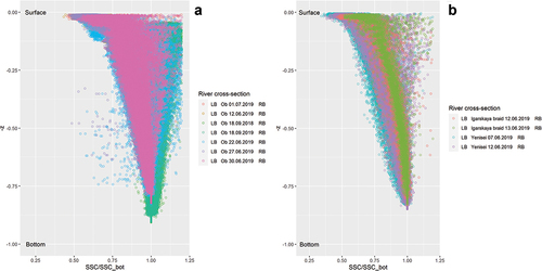
Figure 5. Distribution of the Rouse number (Ro) within river cross-sections by normalized depth (eq. 15(15) $dis{t}_{\mathrm{n}\mathrm{o}\mathrm{r}\mathrm{m}}=\frac{\left|dis{t}_c-dist\right|}{dis{t}_c}$(15) ). Dots show individual ensembles, and lines represent linear approximation for each cross-section.

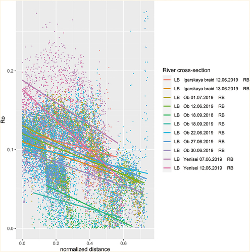
The ADCP dataset also indicates features of Ro number distribution over cross-section by obtaining linear fits from $dis{t}_{\mathrm{n}\mathrm{o}\mathrm{r}\mathrm{m}}$ (average statistics of linear regressions is: Rcor = −0.37, p-value <2.2 × 10⁻¹⁶, n = 327,679). From one profile to another there is a difference between linear regression statistics. Rcor is in the range from −0.74 to −0.21, but all p-values are <2.2 × 10⁻¹⁶ (Table 2). Various ADCP cross-sections demonstrate decrease of Ro towards $dis{t}_{\mathrm{n}\mathrm{o}\mathrm{r}\mathrm{m}}$ = 1 which corresponds to channel maximal depth vertical. This emphasizes the increase of sediment concentration gradients at the central sections of river profiles.

Table 2. Statistical data for the Rouse number (Ro) versus normalized distance (Figure 6).

Profile	r	p-value	n
Yenisei 07.06.2019	−0.48	<2.2×10^−16	38,875
Yenisei 12.06.2019	−0.74	<2.2×10^−16	46,834
Igarskaya braid 12.06.2019	−0.32	<2.2×10^−16	14,554
Igarskaya braid 13.06.2019	−0.37	<2.2×10^−16	9,779
Ob 01.07.2019	−0.52	<2.2×10^−16	39,255
Ob 12.06.2019	−0.48	<2.2×10^−16	34,876
Ob 18.09.2018	−0.36	<2.2×10^−16	7,033
Ob 18.09.2019	−0.21	<2.2×10^−16	4,110
Ob 22.06.2019	−0.21	<2.2×10^−16	60,948
Ob 27.06.2019	−0.47	<2.2×10^−16	43,256
Ob 30.06.2019	−0.41	<2.2×10^−16	28,137

For selected cross-sections total suspended flux was estimated based on ADCP measurement using eqs. 3(3) $SSC=\hspace{0.17em}9.16{\mathrm{e}}^{0.02BI}$(3) –7(7) $SSC=\hspace{0.17em}3.2{\mathrm{e}}^{0.014BI}$(7) and compared with flux estimate which is based on point samples taken during discharge measurement (9 samples over the cross-section). Due to uniform distribution of organic and inorganic suspended load concentrations across the fluvial section, Q_R estimates based on ADCP data are differed from determined by point samples. The difference varies from −3 to −84% (Table 3). As far as ADCP data is homogeneously distributed over cross-section, these differences might be interpreted as accuracy improvement of ADCP-based flux estimate compare to traditional methods.

Table 3. Comparison of suspended sediment load estimates: ADCP versus traditional point-wise sampling method.

		Stream flow discharge, m3/s	QR, ADCP estimate	Number of bins in cross-section	Δ difference (%) between ADCP estimate and estimates based on 9 samples
River	Date		kg/s	n	%
Yenisey at Igarka	08.06.2019	89,200	9,478	50,770	−40.3
	11.06.2019	88,000	9,119	107,775	-
	13.06.2019	83,600	8,958	101,391	−84.8
Ob at Salekhard	27.06.2019	30,600	3,061	139,375	−29.6
	01.07.2019	30,500	2,997	129,024	−52.4
	22.09.2018	11,400	1,618	27,935	−33.3
Kolyma at Cherskiy	3.07.20	9,081	131	11,994	−81
	5.07.20	7,581	105	9,352	−78
	8.07.20	6,727	95	8,407	−3

In average, across the three case studies (Table 3), the application of ADCP processing enhances the sediment flux estimation accuracy up to 51%.

4. Discussion

The results obtained in this study using big data analytics significantly improve knowledge on the specific aspects of sediment transport. Here we discuss these applications in relation to sediment concentration of particulate matter distribution over cross-sections and suspended to bed load partitioning.

This study relies on the calibration method of backscatter intensity to capture sediment concentration. The calibration methods used in our study assume that the echo intensity is governed by average sediment concentration (Sakho et al., 2019). This approach leads to the relationships between SSC and BI characterized by regional equations (eqs. 3(3) $SSC=\hspace{0.17em}9.16{\mathrm{e}}^{0.02BI}$(3) –7(7) $SSC=\hspace{0.17em}3.2{\mathrm{e}}^{0.014BI}$(7) ). Differences between relationships are explained by various particle size distributions. The Lena and Kolyma rivers represent single-mode particle size distribution (silt fraction dominates and form over 40% of suspended sediments), whereas the Ob, Yenisey and Moskva rivers are distinguished by bi-modal particle size distribution (clay and sand fraction transported). This is in line with theoretical (Latosinski, Szupiany, & García et al., 2014) and empirical evidences (Szupiany et al., 2019) which indicate that the sand fraction dominates the backscatter measurements for 600 and 1200 kHz frequencies. For the case study of the Parana River (Szupiany et al., 2019), acoustic method for estimating suspended-sand concentration which considers various classes of suspended sediments resulted in mean deviations within about 40% from sampled concentrations for all survey locations. From our dataset, we compared linear fits between BI and SSC for sand fractions (>50 μm). For that, the full suspended sediment concentration samples were reduced to macro class above 50 μm size, which represents the concentration of sand fraction in the river flow (SSC _>50 μm, mg/l). The results indicated that R² was increasing after changing SSC to SSC _>50 μm at eq. (3)(3) $SSC=\hspace{0.17em}9.16{\mathrm{e}}^{0.02BI}$(3) from 0.28 to 0.45 and for eq. (4)(4) $SSC=\hspace{0.17em}0.59{\mathrm{e}}^{0.382BI}$(4) from 0.59 to 0.67. The particle size analyses were not performed for the remained rivers. This finding confirms the statement that backscatter from the wash-load fraction (typically below 62 μm size) is negligible compared to backscatter from the sand fraction (Latosinski, Szupiany, & García et al., 2014) and should be considered in further studies.

We also attribute the low R² values of the constructed regional BI-SSC relationships to the fact that we had used the raw BI values, not corrected for intrinsic and ambient noise (Szupiany et al., 2019). These findings generally confirm previous research that substantial correlation with corrected backscatter and SSC exists, while raw backscatter intensity does not reasonably predict SSC. Further research is recommended to proceed with corrected BI and to estimate the error values for each of the individual ADCP units used in the study.

Another source of the uncertainties beyond the proposed methodology is related to the field methods of water sampling. Significant errors might occur due to spatial discrepancies occurred between sampled water required for calibration and ADCP measurements. Additionally, ADCP profile shows instantaneous flux distribution which might be significantly varied over short time interval (seconds and minutes) due to vortices and coherent flow structures (Buffin-Bélanger, Roy, & Kirkbride, 2000; Ferguson & Church, 2004).

The important development of the approach presented here is related to the theory of vertical distribution of suspended sediment concentrations. The obtained results here significantly enhance the extension of the large river datasets available for this theory.

The novel semi-empirical equations were found for the case-study rivers. e.g. for the Ob and Yenisey Rivers, the Rouse number is in the range of 0 to 0.2 (Figure 6) evaluated as the average of the Rouse number (1) for each cross-section (totally 15 cross-sections), while the Rouse number is unique for each ensemble. For the Ob and Yenisey we tested dependency for low values of SSC from 56.8 to 88.2 mg/l with mean particles diameter 0.01–0.03 mm (Chalov & Efimov, 2021), and depths from 4 m to 50 m:

(17) $S=S_a{z}^{Ro}$(17)

Assuming the depth a as the depth of the last cell, which was measured by the ADCP (near the bottom non-measured layer), we fitted the sediment concentration vertical distribution curve by adjusting the Ro values. This yields the significant relationships (Rcor = 0.86, p-value <2.9·10⁻⁵, n = 15):

(18) $S=S_a{z}^{-\frac{454}{h_{max}^3}+0.06}$(18)

(19) $Ro=-\frac{454}{h_{max}^3}+0.06$(19)

The Ro dependence from h_max is explained by better mixing of suspended load in the midstream compared to the area near banks. This phenomenon is likely related to the formation of secondary flow velocity cells and activation of new sources of sediment. Also, it can be explained by relatively homogeneous distribution of near-bottom sediment concentrations within cross-section which then requires smaller gradients of sediment concentrations changes at higher depths. This equation is in line with recent theoretical (Julien, 2010; Lane & Kalinske, 1941) and empirical (Zheng, Li, & Feng, 2012) developments, e.g. fractional advection-dispersion equation (FADE) model which was developed to describe anomalous diffusion of sediment (Chen, Sun, & Zhang, 2013).

The ADCP estimates provide a reliable and easily obtained data to calculate suspended sediment load. Simultaneous flow and sediment transport measurements improve procedure of calculating riverine flux which for large rivers is usually based on irregular measurements (Liu, Wang, & Wang et al., 2021; Mu, Zhang, & Chen et al., 2019). The estimates of the suspended flux presented in Table 1 and their discrepancy from estimates using traditional methods are explained mainly by the low spatial resolution of the traditional sediment sampling methods, and generally is corresponding with previously estimated differences (Szupiany et al., 2019). Given that the suspended sediment characteristics of the rivers described in this study are similar to many other sand bed rivers, especially large river systems throughout the world (Chalov, Liu, & Chalov et al., 2018; Latrubesse, 2008), the presented analysis advances efforts to provide more accurate and higher spatial resolution data for fluvial suspended-sediment studies.

Generally, to test the relationship between the observed Ro numbers, we plotted our results (Figure 6) of the relationship between ratio of suspended to total load and Rouse number based on the CSU Laboratory data for the mixed load are from Guy, Simons, and Richardson (Guy, Simons, & Richardson, 1966) and for small rivers located within Moscow area conducted within this study. For that, both with ADCP suspended load fluxes, bed load fluxes (q_G) were estimated using equations (11)(11) $q_G=\epsilon {\rho }_{s}Vh{\left(\frac{{\mathrm{d}}_{50}\hspace{0.17em}}{h}\right)}^{1.2}(M_e{)}^{\eta }$(11) –(13(13) $Q_G=\underset{0}{\overset{B}{\int }}{q}_{G}dB$(13) ).

Figure 6. The observed values of Ro and partitioning conditions of sediment transport R/(R+G) under various Rouse and $\frac{h}{d_{50}}$. Small rivers, h < 0.5 m – data from Guy, Simons, and Richardson (1966) and Julien (2010) and measurements at the Moskva River conducted within this study. Theoretical lines are from Einstein integral (Shah-Fairbank & Julien, 2015).

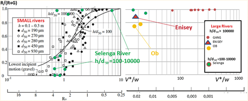
Further partitioning between bed load and sediment load was assessed as R/G = $\frac{\hspace{0.17em}{Q}_R\hspace{0.17em}}{\hspace{0.17em}{Q}_R+\hspace{0.17em}{Q}_G}$ for each transect. Lines shown are those from the Einstein Integrals of Guo and Julien as obtained by Shah-Fairbank (Shah-Fairbank & Julien, 2015) for h/d₅₀ 100 and 100,000. It can be clearly seen that measured conditions in the Selenga River generally close to fit line for the rivers at h/d₅₀ = 100,000 (Figure 6). At the same time this shows that one can obtain an extremely large variability in sediment concentration and thus R/(R+G) ratio in deep sand-bed rivers when the Rouse number is fairly large (Ro >0.5). Case study on the Selenga River is quite instructive in this regard, which reflects conditions of abrupt shift from mixed and bed load dominated channel (Ro <2) to suspended sediment dominated channel (Ro >2). The average Rouse number presented in Figure 6 can be significantly varied between single verticals, e.g. for the measurement on the Ob River done at 01/07/19 the average Rouse number 0.2 corresponds to changes from 0.01 at the midstream up to 0.8 at the near-bank area. On the large rivers (with depth over 10 m and $\frac{h}{d_{50}}\hspace{0.17em}$ >100,000) suspended load dominates ($Q_R$/($Q_R$+$Q_G$) = 0.5–0.75) under broad hydraulic conditions Ro (Ro = 0.001–2). Here we plotted our measurements at the Ob and Yenisey rivers and similar studies done at the Ganga River (Lupker, France-Lanord, & Lavé et al., 2011). These results for the first time indicate that partitioning between bed and suspended load on small and large rivers are similar but subjected to scale effects. Further studies based on ADCP datasets will provide a novel knowledge on the total sediment flux hydrodynamic partitioning which is one of the vaguest questions in river hydrology (Chalov, Moreido, & Sharapova et al., 2020; Turowski, Rickenmann, & Dadson, 2010). If the accuracy of ADCP application is considered, presented here big data processing approach will lead to tremendous enhancement of suspended sediment data (Lehotský, Rusnák, Kidová, & Dudžák, 2018; Pomázi & Baranya, 2020) and contribute novel concepts to understanding of suspended sediment fluxes behavior and estimates within the river profiles.

5. Conclusions

The ADCP big data analytics provides a fundamental shift in suspended sediment studies as a cost-effective and accurate technology. The main conclusions of the study are as follows:

1. We have developed an integrated freely available open-source tool consisting of 3 R-language codes for ADCP data processing which enables sediment concentration assessment within cross-sections of large rivers.

2. The ADCP big data provide novel approach for flow hydraulics and sediment distribution studies on large rivers. The novel semi-empirical equation for sediment concentration was parameterized for the sandy (average diameter 0.01–0.03 mm) large rivers (average depths varying from 4 to 50 m).

3. The results derived in this study are used to improve accuracy of fluvial sediment transport estimates which are required to improve fundamental understanding of land-ocean coupling. Acoustic technologies show potential for estimating suspended load transport both quickly and accurately using big data on sediment concentrations. Another important output of our study is the understanding that specific methodological requirements should be fulfilled under processing ADCP data: e.g. raw backscatter values are not recommended as far as they do not reasonably predict SSC.

It is shown that suspended load and the sediment concentration profiles are well explained by the Rouse type equation, which allows us to estimate the instantaneous hydrodynamic partitioning of the sediment flux. The sediment flux estimates obtained by using this approach appear to be realistic, and the ADCP datasets provide a novel knowledge on partitioning of suspended and bed load.

Disclosure statement

No potential conflict of interest was reported by the author(s).

Data availability statement

All data processed in this study was derived by authors field work by the ADCP owned by the Lomonosov Moscow State University. Authors consent that all datasets (including video recordings) are open and can be used for research and educational activities. The data that support the findings of this study are openly available in public repository and can be downloaded from https://doi.org/10.1080/20964471.2022.2116834.

Additional information

Funding

The study is done under implementation of Russian Scientific Foundation support (project 21-17-00181). Additionally, field studies at the Selenga River were supported by Russian Fund for Basic Research (project 18-05-60219), field studies at the Lena River – by Russian Scientific Foundation support (project 21-17-00181), field studies at the Moscow River catchment – within Scientific Foundation project 19-77-30004. The analytical experiments were supported by the Ministry of Science and Higher Education of Russian Federation under the Agreement 075-15-2021-574. Also, this paper has been supported by the Kazan Federal University Strategic Academic Leadership Program.

Notes on contributors

Sergey Chalov

Sergey R. Chalov received his M.S. in Fluvial Processes and Hydrology from the Faculty of Geography of the Lomonosov Moscow State University (LMSU) in 2004 and 2007, respectively. After receiving his Ph.D., he worked at the Hydrology Department of the Faculty of Geography, since 2018, as an Associate professor. In October 2021 he defended habilitation thesis on the topic “River sediments and fluvial systems”.

Vsevolod Moreido

Sergey R. Chalov received his M.S. in Fluvial Processes and Hydrology from the Faculty of Geography of the Lomonosov Moscow State University (LMSU) in 2004 and 2007, respectively. After receiving his Ph.D., he worked at the Hydrology Department of the Faculty of Geography, since 2018, as an Associate professor. In October 2021 he defended habilitation thesis on the topic “River sediments and fluvial systems”.

Vsevolod M. Moreido received his M.S. in Hydrology from the Faculty of Geography of the Lomonosov Moscow State University (LMSU) in 2004 and Ph.D in Hydrology from the Water Problems Institute of Russian Academy of Sciences in 2015. After receiving his Ph.D., he worked at the Flood Risk Laboratory of the Water Problems Institute of Russian Academy of Sciences as a senior researcher.

Aleksandra S. Chalova received her M.S. and Ph.D in Fluvial Processes and Hydrology from the Faculty of Geography of the Lomonosov Moscow State University (LMSU) in 2006 and 2009, respectively. After receiving her Ph.D., she worked at the Laboratory of erosion and channel processes of the Faculty of Geography as a junior researcher.

Victor Ivanov

Victor V. Ivanov received his M.S. in 2022 and now he is a Ph.D student at the Hydrology Department of the Faculty of Geography of the Lomonosov Moscow State University (LMSU).

Aleksandra Chalova

Aleksandra S. Chalova received her M.S. and Ph.D in Fluvial Processes and Hydrology from the Faculty of Geography of the Lomonosov Moscow State University (LMSU) in 2006 and 2009, respectively. After receiving her Ph.D., she worked at the Laboratory of erosion and channel processes of the Faculty of Geography as a junior researcher.

References

- Agrawal, Y. C., & Hanes, D. M. (2015). The implications of laser-diffraction measurements of sediment size distributions in a river to the potential use of acoustic backscatter for sediment measurements. Water Resources Research, 51(11), 8854–8867. doi:10.1002/2015WR017268
- Aleixo, R., Guerrero, M., Nones, M., & Ruther, N. (2020). Applying ADCPs for Long-Term Monitoring of SSC in Rivers. Water Resources Research, 56(1). doi:10.1029/2019WR026087
- Bityukova, V. R., & Koldobskaya, N. A. (2018). Environmental factors and constraints in the development of the new territory of Moscow (so-called «new Moscow»). Geography, Environment, Sustainability, 11(2), 46–62. doi:10.24057/2071-9388-2018-11-2-46-62
- Boldt, J. A. (2015). From mobile ADCP to high-resolution SSC; a cross-section calibration tool—proceedings of the 3d Joint Federal Interagency Conference on Sedimentation and Hydrologic Modeling, April 19-23, Reno, Nev. 1258–1260. http://acwi.gov/sos/pubs/3rdJFIC/Proceedings.pdf
- Boldt, J. A., Czuba, J. A., Straub, T. D., Curran, C. A., Szupiany, R. N., & Oberg, K. A. (2012). Estimation of suspended-sediment concentration from down-looking acoustic Doppler current profilers using an acoustic backscatter calibration procedure and MATLAB-based tool—Proceedings of the Hydraulic Measurements and Experimental Methods Conference, August 12-15 , Utah.
- Bouchez, J., Métivier, F., Lupker, M., et al. (2011). Prediction of depth-integrated fluxes of suspended sediment in the Amazon River: Particle aggregation as a complicating factor. Hydrological Processes, 25, 778–794. doi:10.1002/hyp.7868
- Buffin-Bélanger, T., Roy, A. G., & Kirkbride, A. D. (2000). On large-scale flow structures in a gravel-bed river. Geomorphology, 32(3–4), 417–435. doi:10.1016/S0169-555X(99)00106-3
- Chalov, S. R., & Efimov, V. A. (2021). Mechanical composition of suspended sediments: Classifications, characteristics, spatial variability. Vestnik Geography, 4, 91–103.
- Chalov, S., Golosov, V., Tsyplenkov, A., et al. (2017). A toolbox for sediment budget research in small catchments. Geography, Environment, Sustainability, 10(4), 43–68. doi:10.24057/2071-9388-2017-10-4-43-68
- Chalov, S. R., Liu, S., Chalov, R. S., et al. (2018). Environmental and human impacts on sediment transport of the largest Asian rivers of Russia and China. Environmental Earth Sciences, 77, 1–14. doi:10.1007/s12665-018-7448-9
- Chalov, S., Moreido, V., & Ivanov, V. et al. (2022). Assessing suspended sediment fluxes with acoustic doppler current profilers: Case study from large rivers in Russia [Data set]. Zenodo. 10.5281/zenodo.6815844
- Chalov, S., Moreido, V., Sharapova, E., et al. (2020). Hydrodynamic Controls of Particulate Metals Partitioning Along the Lower Selenga River—Main Tributary of the Lake Baikal. Water, 12(5), 1345. doi:10.3390/w12051345
- Chen, D., Sun, H. G., & Zhang, Y. (2013). Fractional dispersion equation for sediment suspension. Journal of Hydrology, 491, 13–22. doi:10.1016/j.jhydrol.2013.03.031
- Collins, A. L., & Walling, D. E. (2007). The storage and provenance of fine sediment on the channel bed of two contrasting lowland permeable catchments, UK. River Research and Applications, 23(4), 429–450. doi:10.1002/rra.992
- Davis, B. E. (2005). A guide to the proper selection and use of federally approved sediment and water-quality samplers. U.S. Geol. Surv. Open File Rep. 20 http://pubs.usgs.gov/of/2005/1087/pdf/OFR_2005-1087.pdf]
- Deines, K. L. (1999). Backscatter estimation using broadband acoustic Doppler current profilers. Proceedings of the IEEE Working Conference on Current Measurement. 10.1109/ccm.1999.755249
- Diplas, P., Kuhnle, R., & Gray, J., et al. (2008). Sediment Transport Measurements. In: M. Garcia, ed. Sedimentation Engineering. American Society of Civil Engineers, Reston, VA, 307-353.
- Dominguez Ruben, L. G., Szupiany, R. N., Latosinski, F. G., Lopez Weibel, C., Wood, M., & Boldt, J. (2020). Acoustic Sediment Estimation Toolbox (ASET): A software package for calibrating and processing TRDI ADCP data to compute suspended-sediment transport in sandy rivers. Computer and Geosciences, 140, 104499. doi:10.1016/j.cageo.2020.104499
- Edwards, T. K., & Glysson, G. D. (1999). Field methods for measurement of fluvial sediment. In Techniques of Water-Resources Investigations of the U.S. Geological Survey: Book 3, Application of Hydraulics. Reston, VA: U.S. Geological Survey, 89.
- Efimov, V. A., Chalov, S. R., & Efimova, L. E., et al. (2019). Impact of mining activities on the surface water quality (case study of Khibiny mountains, Russia). IOP Conference Series: Earth and Environmental Science, Bristol, UK, England.
- Elçi, Ş., Aydın, R., & Work, P. A. (2009). Estimation of suspended sediment concentration in rivers using acoustic methods. Environmental Monitoring and Assessment, (1–4), 159. doi:10.1007/s10661-008-0627-5
- Ferguson, R. I., & Church, M. (2004). A Simple Universal Equation for Grain Settling Velocity. Journal of Sedimentary Research, 74(6), 933. doi:10.1306/051204740933
- García, M. H. (2008). Sediment transport and morphodynamics, chap. 2, In: M. H. García, ed. Sedimentation Engineering: Processes, Measurements, Modeling, and Practice: ASCE Manuals and Reports on Engineering Practice No.110. Reston, Va: American Society of Civil, 21–163.
- Gartner, J. W. (2004). Estimating suspended solids concentrations from backscatter intensity measured by acoustic Doppler current profiler in San Francisco Bay, California. Marine Geology, 211(3–4), 169–187. doi:10.1016/j.margeo.2004.07.001
- Graf, W. H., & Cellino, M. (2002). Suspension flows in open channels; experimental study. Journal of Hydraulic Research, 40(4), 435–447. doi:10.1080/00221680209499886
- Gray, J. R., & Gartner, J. W. (2009). Technological advances in suspended-sediment surrogate monitoring. Water Resources Research, 45(4). doi:10.1029/2008WR007063
- Grishanin, K. V. (1972). Theory of the fluvial process. Transport, Moscow.
- Guerrero, M., & Federico, V. (2018). Suspended sediment assessment by combining sound attenuation and backscatter measurements – analytical method and experimental validation. Advances in Water Resources, 113, 167–179. doi:10.1016/J.ADVWATRES.2018.01.020
- Guerrero, M., Rüther, N., Haun, S., & Baranya, S. (2017). A combined use of acoustic and optical devices to investigate suspended sediment in rivers. Advances in Water Resources, 102, 1–12. doi:http://dx.doi.org/10.1016/j.advwatres.2017.01.008
- Guerrero, M., Szupiany, R. N., & Latosinski, F. (2013). Multifrequency acoustics for suspended sediment studies: An application in the Parana River. Journal of Hydraulic Research, 51(6), 696–707. doi:10.1080/00221686.2013.849296
- Guy, H. P., Simons, D. B., & Richardson, E. V. (1966). Summary of Alluvial Channel Data from Flume Experiments, 1956-61, 462-I. US Geology Survey, 1–104.
- Hackney, C. R., Darby, S. E., Parsons, D. R., Leyland, J., Aalto, R., Nicholas, A. P., & Best, J. L. (2018). The influence of flow discharge variations on the morphodynamics of a diffluence–confluence unit on a large river. Earth Surface Processes and Landforms, 43(2), 349–362. doi:10.1002/ESP.4204
- Hanes, D. M. (2012). On the possibility of single-frequency acoustic measurement of sand and clay concentrations in uniform suspensions. Continental Shelf Research, 46, 64–66. doi:10.1016/J.CSR.2011.10.008
- Hauer, R. F., & Lamberti, G. A. (2017). Methods in Stream Ecology (Vol. 1, p. 506). Ecosystem Structure.
- Holdaway, G. P., Thorne, P. D., Flatt, D., Jones, S. E., & Prandle, D. (1999). Comparison between ADCP and transmissometer measurements of suspended sediment concentration. Continental Shelf Research, 19(3), 421–441. doi:10.1016/S0278-4343(98)00097-1
- Horowitz, A. (1985). A primer on trace metal-sediment chemistry. US Geology Survey Water-Supply Paper, 2277, 67.
- Julien, P. Y. (2010). Erosion and sedimentation. Cambridge, England: Cambridge University Press.
- Kemp, P., Sear, D., Collins, A., et al. (2011). The impacts of fine sediment on riverine fish. Hydrological Processes, 25(11), 1800–1821. doi:10.1002/hyp.7940
- Kirillov, P. L., Makhrova, A. G., & Nefedova, T. G. (2019). Current Trends in Moscow Settlement Pattern Development: A Multiscale Approach. Geography, Environment, Sustainability, 12(4), 6–23. doi:10.24057/2071-9388-2019-69
- Lane, E. W., & Kalinske, A. A. (1941). Engineering calculations of suspended sediment. Eos, Transactions American Geophysical Union, 22(3), 603–607. doi:10.1029/TR022i003p00603
- Latosinski, F. G., Szupiany, R. N., García, C. M., et al. (2014). Estimation of Concentration and Load of Suspended Bed Sediment in a Large River by Means of Acoustic Doppler Technology. Journal of Hydraulic Engineering, 140(7). doi:10.1061/(ASCE)HY.1943-7900.0000859
- Latrubesse, E. M. (2008). Patterns of anabranching channels: The ultimate end-member adjustment of mega rivers. Geomorphology, 101(1–2), 130–145. doi:10.1016/j.geomorph.2008.05.035
- Lehotský, M., Rusnák, M., Kidová, A., & Dudžák, J. (2018). Multitemporal assessment of coarse sediment connectivity along a braided-wandering river. Land Degradation and Development, 29(4), 1249–1261. doi:10.1002/ldr.2870
- Liu, S., Wang, P., & Wang, T., et al. (2021). Characteristic analysis of organic carbon output and its affecting factors of Arctic rivers in Siberia. Dili Xuebao/acta Geographica Sinica, 76(5), 1065–1077. doi:10.11821/dlxb202105002
- Lupker, M., France-Lanord, C., & Lavé, J., et al. (2011). A Rouse-based method to integrate the chemical composition of river sediments: Application to the Ganga basin. Journal of Geophysical Research: Earth Surface, 116(F4). 10.1029/2010JF001947
- Lynds, R. M., Mohrig, D., Hajek, E. A., & Heller, P. L. (2014). Paleoslope reconstruction in sandy suspended-load-dominant rivers. Journal of Sedimentary Research, 84(10), 825. doi:10.2110/jsr.2014.60
- Moore, S. A., Le, C. J., Hurther, D., & Paquier, A. (2013). Using multi-frequency acoustic attenuation to monitor grain size and concentration of suspended sediment in rivers. The Journal of the Acoustical Society of America, 133(4), 1959. doi:10.1121/1.4792645
- Mueller, D. S., & Wagner, C. D. (2009). Measuring discharge with acoustic Doppler current profilers from a moving boat. Geological Survey Techniques and Methods, 3–A22.
- Mullison, J. (2017). Backscatter Estimation Using Broadband Acoustic Doppler Current Profilers. Conference: Hydraulic Measurements & Experimental Methods. Durham, NH., 1–6.
- Mu, C., Zhang, F., & Chen, X., et al. (2019). Carbon and mercury export from the Arctic rivers and response to permafrost degradation. Water Research, 161, 54–60. doi:10.1016/j.watres.2019.05.082
- Nie, S., Sun, H., & Zhang, Y., et al. (2017). Vertical Distribution of Suspended Sediment under Steady Flow: Existing Theories and Fractional Derivative Model. Discrete Dynamics in Nature and Society, ID, 5481531. doi:10.1155/2017/5481531
- Pomázi, F., & Baranya, S. (2020). Comparative assessment of fluvial suspended sediment concentration analysis methods. Water, 12(3), 873. doi:10.3390/w12030873
- Rstudio Team. (2019). RStudio: Integrated development for R. RStudio, Inc., Boston MA. RStudio
- Sakho, I., Dussouillez, P., Delanghe, D., Hanot, B., Raccasi, G., Tal, M. … Radakovitch, O. (2019). Suspended sediment flux at the Rhone River mouth (France) based on ADCP measurements during flood events. Environmental Monitoring and Assessment, 191, 508. doi:10.1007/s10661-019-7605-y
- Sassi, M. G., Hoitink, A. J. F., & Vermeulen, B. (2012). Impact of sound attenuation by suspended sediment on ADCP backscatter calibrations. Water Resources Research, 48(9). doi:10.1029/2012WR012008
- Shah-Fairbank, S. C., & Julien, P. Y. (2015). Sediment load calculations from point measurements in sand-bed rivers. International Journal of Sediment Research, 30(1), 1–12. doi:10.1016/S1001-6279(15)60001-4
- Sievert, C. (2020). Interactive Web-Based Data Visualization with R, plotly, and shiny. NY: Chapman and Hall. doi:10.1201/9780429447273
- Szupiany, R. N., Amsler, M. L., Parsons, D. R., & Best, J. L. (2009). Morphology, flow structure, and suspended bed sediment transport at two large braid-bar confluences. Water Resources Research, 45(5). doi:10.1029/2008WR007428
- Szupiany, R. N., Lopez Weibel, C., Guerrero, M., Latosinski, F., Wood, M., Dominguez Ruben, L., & Oberg, K. (2019). Estimating sand concentrations using ADCP-based acoustic inversion in a large fluvial system characterized by bi-modal suspended-sediment distributions. Earth Surface Processes and Landforms, 44(6), 1295–1308. doi:10.1002/esp.4572
- Szupiany, R. N., Lopez Weibel, C., Latosinki, F., Dominguez Ruben, L., Amsler, M., & Guerrero, M., (2016). Sediment concentration measurements using ADCPs in a large river: Evaluation of acoustic frequency and grain size. In Proceedings of the International Conference on Fluvial Hydraulics. 10.1201/9781315644479-243
- Tereshina, M., Erina, O., Sokolov, D., et al. (2020). Nutrient dynamics along the Moskva River under heavy pollution and limited self-purification capacity. In: E3S Web of Conferences
- Thorne, P. D., & Hanes, D. M. (2002). A review of acoustic measurement of small-scale sediment processes. Continental Shelf Research, 22(4), 603–632. doi:10.1016/S0278-4343(01)00101-7
- Thorne, P. D., & Meral, R. (2008). Formulations for the scattering properties of suspended sandy sediments for use in the application of acoustics to sediment transport processes. Continental Shelf Research, 28(2), 309–317. doi:10.1016/J.CSR.2007.08.002
- Thorne, P. D., Vincent, C. E., Hardcastle, P. J., Rehman, S., & Pearson, N. (1991). Measuring suspended sediment concentrations using acoustic backscatter devices. Marine Geology, 98(1), 7–16. doi:10.1016/0025-3227(91)90031-X
- Topping, D. J., & Wright, S. A. (2016). Long-Term continuous acoustical suspended-sediment measurements in rivers – Theory, application, bias, and error. Professional Paper 1823. 10.3133/PP1823
- Townsend, C. R., Uhlmann, S. S., & Matthaei, C. D. (2008). Individual and combined responses of stream ecosystems to multiple stressors. The Journal of Applied Ecology, 45(6), 1810–1819. doi:10.1111/j.1365-2664.2008.01548.x
- Turowski, J. M., Rickenmann, D., & Dadson, S. J. (2010). The partitioning of the total sediment load of a river into suspended load and bedload: A review of empirical data. Sedimentology, 57(4), 1126–1146. doi:10.1111/j.1365-3091.2009.01140.x
- van Rijn, L. C. (2007). Unified view of sediment transport by currents and waves. I: Initiation of motion, bed roughness, and bed-load transport. Journal of Hydraulic Engineering, 133(6), 649–667. doi:10.1061/(ASCE)0733-9429(2007)133:6(649)
- Venditti, J. G., Church, M., Attard, M. E., & Haught, D. (2016). Use of ADCPs for suspended sediment transport monitoring: An empirical approach. Water Resources Research, 52(4), 2715–2736. doi:10.1002/2015WR017348
- Vihma, T., Uotila, P., & Sandven, S., et al. (2019). Towards an advanced observation system for the marine Arctic in the framework of the Pan-Eurasian Experiment (PEEX). Atmospheric Chemistry and Physics, 19(3), 1941–1970. doi:10.5194/acp-19-1941-2019
- Walling, D. E. (2006). Human impact on land–ocean sediment transfer by the world’s rivers. Geomorphology, 79(3–4), 192–216. doi:10.1016/j.geomorph.2006.06.019
- Wall, G. R., Nystrom, E. A., & Litten, S. (2006). Use of an ADCP to compute suspended-sediment discharge in the tidal Hudson River. New York: Scientific Investigations Report 2006-5055, 26.
- Wang, Y., Chu, Y. S., Lee, H. J., Han, C. K., & Oh, B. C. L. (2005). Estimation of suspended sediment flux from acoustic Doppler current profiling along the Jinhae Bay entrance. Acta Oceanologica Sinica, 24(2), 16–27.
- Wang, Y., Gao, S., & Li, K. (2000). A preliminary study on suspended sediment concentration measurements using an ADCP mounted on a moving vessel. Chinese Journal of Liminology and Oceanology, 18(2), 183–189. doi:10.1007/BF02842579
- Wang, Y., Pan, S., & Wang, H. V. (2006). Measurements and analysis of water discharges and suspended sediment fluxes in Changjiang Estuary. Acta Geographica Sinica – Chinese Edition, 61(1), 35–46. doi:10.11821/xb200601004
- Wickham, H., Averick, M., & Bryan, J., et al. (2019). Welcome to the Tidyverse. Journal of Open-Source Software 4. 10.21105/joss.01686
- Wood, M. S., Szupiany, R., Boldt, J., Straub, T., & Domanski, M. (2019). Measuring suspended sediment in sand-bedded rivers using down-looking acoustic Doppler current profilers. Proceedings of the SEDHYD 2019 Conference on Sedimentation and Hydrologic Modeling, June 24-28. Reno, 16 p.
- Zheng, J., Li, R., & Feng, Q. (2012). Vertical distribution of nearshore sediment concentration. Applied Mechanics and Materials, 170–173, 2272–2275.
- Zheng, J., Li, R., Feng, Q., & Lu, S. (2013). Vertical profiles of fluid velocity and suspended sediment concentration in nearshore. International Journal of Sediment Research, 28(3), 406–412. doi:10.1016/S1001-6279(13)60050-5