An interactive tool for visualization and prediction of solar radiation and photovoltaic generation in Colombia

ABSTRACT

This paper presents the building process of an interactive instrument called the Colombian Solar Atlas able to easily visualize meteorological data but also assess the current and future potentials of solar photovoltaic generation throughout the whole territory of Colombia, South America. This new tool is based on two different meteorological databases. The first one is done with historical data extracted from satellite imagery information, and the other one corresponds to data issues from regional-scale climate change projection models. The satellite database was validated with different in-situ measurements. The Colombian Solar Atlas uses basic and advanced photovoltaic generation models to estimate the generation of a custom solar installation. With this tool, a user selects a point on the map and can have directly pertinent information to search for an optimal location with a spatial resolution of 4 km². This tool is the first open interactive online tool particularly adapted to study the photovoltaic power potential in Colombia, considering the country’s needs and native language.

KEYWORDS:

• Solar atlas
• PV power potential
• climate change
• Colombia
• data validation

1. Introduction

Colombia, located in South America, receives abundant solar irradiation with an average of 4.5 $kWh/m^2/d$, which is above the world average of 3.9 $\mathrm{k}\mathrm{W}\mathrm{h}/{\mathrm{m}}^2/\mathrm{d}$. This average solar irradiation remains almost constant throughout the year, making Colombia an ideal place to implement solar photovoltaic projects (Abril et al., 2021). The Colombian government has implemented a law to stimulate the implementation of small- and large-scale PV systems by providing tax incentives (UPME, 2014). However, despite the government’s efforts to promote PV installations, the lack of a robust and easy-to-access database of meteorological information makes it challenging to conduct feasibility analyses of PV installations and assess their power capacity. In-situ measurements of meteorological data are provided in Colombia by the Institute of Hydrology, Meteorology, and Environmental Studies (IDEAM). However, there are few meteorological stations in the Colombian territory, and the quality of the data is affected due to a lack of maintenance and sensor calibration. Although some websites attempt to provide PV production estimates, there is no specialized tool that considers the country’s needs, the user’s requirements, and the user’s native language. Therefore, a tool that takes into account these requirements will potentially boost solar PV projects in the country.

To solve this problem, we have created an interactive tool with accessible information about meteorological variables and PV power potential. This tool, called Colombian Solar Atlas¹, provides an interactive map that displays:

● Historical data for the period ranging from 1998–2019 obtained from the National Renewable Energy Laboratory (NREL) for six meteorological variables: global horizontal irradiance (GHI), direct normal irradiance (DNI), diffuse horizontal irradiance (DHI), solar zenith angle, wind speed, and ambient temperature. This database was validated with in-situ measurements provided by the Institute of Hydrology, Meteorology, and Environmental Studies (IDEAM).

● Data from regional-scale climate change scenarios for the period 2070–2099 obtained from the Coordinated Regional Downscaling Experiment (CORDEX) for three meteorological variables: surface-downwelling shortwave radiation, wind speed, and ambient temperature under two climate change scenarios.

● A photovoltaic generation calculator that allows users to estimate the possible PV power produced by a custom PV system at a specific location. A basic model provides default parameters for the PV system, and all the PV parameters can be customized through the advanced model.

Table 1 compares different atlases presented in the literature with our Atlas. This is the first interactive online tool that allows users to study the PV power potential in Colombia based on a robust database and considering climate change projections. This interactive tool will enable investors to assess the current and future potentials of photovoltaic solutions. The Colombian Solar Atlas is an interactive tool designed not only for the scientific community but also for the general audience. Figure 1 presents the methodology for the development of the Colombian Solar Atlas. The first step is data collection, followed by data validation. We then estimate the PV power potential and develop the Solar Atlas. Finally, the Solar Atlas is deployed online. The same methodology can be applied to other countries by changing the database to the corresponding one.

Figure 1. The flowchart of Colombian Solar Atlas.

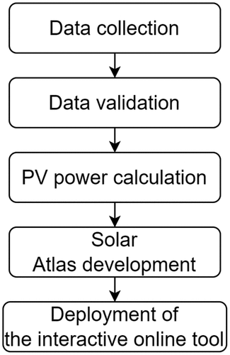
Table 1. Comparison between other atlases and the Colombian Solar Atlas.

	PVGIS	Global Solar Atlas	Chilean Atlas	IDEAM Atlas	Proposed Solar Atlas
Datasets used	ERA5, NSRDB, SARAH	SOLAR-GIS	GOES EAST	In-situ data	NSRDB and CORDEX
Analyzed time period	2005–2015	1994–2020	2004–2016	2015	1998–2019 and 2070–2099
Visualize different heat maps		✓		✓	✓
Allows to download information	✓	✓	✓	✓	✓
Allows to calculate PV potential for different models	✓		✓		✓
Shows meteorological variables	✓	✓	✓		✓
Allows the user to choose different years	✓				✓
Shows maps for climate change scenarios					✓

This paper is organized as follows. In Section 2, we present previous work and a comparison between several already developed solar atlases and the Colombia Solar Atlas. We then explain in Section 3 the data collection, pre-processing, and validation process to generate the interactive map with historical data. Section 4 describes the data collection process to develop the interactive map with climate change scenarios at a regional scale, followed by Section 5, which presents the models used to estimate the photovoltaic generation potential. We end this paper with a conclusion and future work in Section 6, and the technical description of the Solar Atlas and its functionalities in Appendix A and Appendix B, respectively.

2. Previous work and contribution of the paper

Over the last years, multiple tools have been developed in an effort to collect and allow users to visualize meteorological data in an easy and accessible way. One of the main tools is provided by NREL, which consists of a data viewer tool that provides worldwide meteorological data, multiple base maps, and spatial layers that can be accessed through a website (National Renewable Energy Laboratory, 2022).

On a continent-scale, different organizations have created different solar atlases. PVGIS was developed by the European Commission's Joint Research Centre. The PVGIS Atlas (European Commission Joint Research Centre, 2019) uses different datasets, such as SARAH, which has been calculated by the Satellite Application Facility on Climate Monitoring (CM SAF), NSRDB, in collaboration with the National Renewable Energy Laboratory (NREL), and ERA5, a new reanalysis product from the European Centre for Medium-Range Weather Forecasts (ECMWF). SARAH data cover Europe, Africa, and most of Asia, NSRDB covers North and Central America, and ERA5 is available only for Europe. The data provided by these atlases correspond to the years 2005 to 2015 (European Comission, 2020a). PVGIS atlas calculates the performance of a custom PV system, allowing the user to enter different values regarding the solar panel for different panel configurations. Even though it allows the user to obtain the monthly average for GHI, DNI, DHI, temperature, and hourly solar irradiance (European Comission, 2020b), the heat map only shows the average solar irradiance.

Another atlas on a continent-scale is the Global Solar Atlas, developed by the World Bank and the International Finance Corporation to support the scale-up of solar power in different countries. The main purpose of this atlas is to provide quick access to potential PV data, and global solar resources (The World Bank, 2017a) and allow countries and communities to transform their energy infrastructure and step up their low-carbon energy transition (Suri et al., 2020). This atlas uses information obtained through SOLARGIS, a paid platform that provides meteorological data for solar energy investments. SOLARGIS is specially focused on project development and operational projects. Unfortunately, this dataset does not contain information for all parts of the world (SOLARGIS, 2021).

The Global Solar Atlas has different functions regarding solar variables visualization and estimated PV power potential through interactive maps. It provides annual average values for PV power output, DNI, GHI, DHI, global tilted irradiance at an optimum angle, an optimum tilt of PV modules, air temperature, and terrain elevation. The user can select a point on the map or search for a specific location. The atlas also has a PV energy yield calculator, in which the long-term energy yield for a custom PV system can be calculated. The atlas shows daily and annual averages of the estimated PV production. A user can download an image of a heat map given a specific region or country for the GHI, DNI, and PV power potential (The World Bank, 2017b). It is not possible to select a particular year for data display.

On a country scale, one of the most complete databases and tools has been developed by the University of Chile in partnership with the Chilean government (Molina et al., 2017). The Chilean Ministry of Energy developed several tools in an effort to provide an accessible and free way of analyzing Chile’s renewable resources. In particular, the Solar Explorer (Chilean Ministry of Energy, 2017) is a website that provides an interactive map in which a user can select a specific point and visualize data such as solar irradiance, cloudiness, ambient temperature, wind speed, and elevation. This tool also includes a photovoltaic generation simulator, which allows the user to calculate the electricity generation of a photovoltaic system as if it was installed at a specific point. All data can be visualized in graphs showing the daily and annual averages of photovoltaic generation and other meteorological variables. The user can compare two graphs from different points at the same time. The database provides hourly data from 2004 until 2016 at 90 meters spatial resolution, using cloud detection and characterization methods based on data from GOES EAST satellite, as well as transfer models such as NASA’s CLIRAD-SW, to estimate the clear sky solar irradiance.

Finally, the Colombian Institute of Hydrology, Meteorology, and Environmental Studies (IDEAM) developed the Solar, Ultraviolet, and Ozone Radiation Atlas. This tool provides a set of maps representing the monthly and yearly distribution of global horizontal irradiance, sunshine, number of days without sunshine, ultraviolet radiation, total ozone, and regional analysis of the annual average behavior for each variable in the year 2015. The data are measured from 230 global irradiance sensors, and 497 sunshine sensors (Institute of Hydrology, Meteorology and Environmental Studies, 2022). This tool only has information for some of the main cities in Colombia in 2015 and does not include data for other meteorological variables such as wind speed or ambient temperature.

Our Solar Atlas attempts to take the best of the other atlases presented in the literature to obtain a robust tool to assess the PV power potential for the entire Colombian territory. Table 1 compares the different atlases found in the literature and our proposed interactive tool. Our proposed Solar Atlas is the only atlas that contains all the features presented in Table 1 in Colombia.

3. Map with historical data

3.1. Data collection

We use historical data from the National Solar Radiation Database (NSRDB) (Sengupta et al., 2018a). This database collects meteorological data such as GHI, DNI, DHI, temperature, and wind speed. The latest version of the database offers gridded data from 1998 to 2019, with a 4 km $\times$ 4 km spatial resolution and a temporal resolution of 30 minutes, generated with a physical solar model (PSM). This model computes solar irradiance from different satellite data, specifically by measuring aerosol, water vapor, and other meteorological properties combined with satellite-derived cloud properties in the Fast All-sky Radiation Model for Solar applications (FARMS) (Gelaro et al., 2017).

Since NSRDB uses two-step physical models, different satellites are required to extract data. Figure 2 shows a flowchart of the two-step PSM to calculate solar irradiance from satellite data. NSRDB uses data from the Geostationary Operational Environmental Satellite (GEOES) and Advanced Very High-Resolution Radiometer (AVHRR), developed by the National Oceanic and Atmospheric Administration (NOAA), that retrieved cloud products at 4 km $\times$ 4 km for every 30 minutes. The PSM has used this information to produce cloud-sky solar irradiance since 1998.

Figure 2. The flowchart of the NREL Physical Solar Model (PSM).

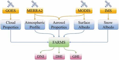
Based on monthly Moderate Resolution Imaging Spectroradiometer (MODIS) data, in combination with the Modern-Era Retrospective Analysis for Research and Applications version 2 (MERRA-2) aerosol dataset, the PSM uses the data for the aerosol optical depth (AOD). Over the arid areas (southern and western United States, and northern Mexico), the aerosol optical depth is obtained using an optimal linear combination of the satellites MERRA-2 and MODIS. When MODIS data are unavailable, only data from MERRA-2 is used. Over the vegetation or urban areas (eastern and northern United States, Canada, southern Mexico, and Central America), the aerosol optical depth is obtained using only data from MERRA-2 since it has similar accuracy as MODIS, which presents unavailable data occasionally (Sengupta et al., 2018a).

NSRDB provides atmospheric and land properties, such as atmospheric profile, wind direction and speed, snow depth, surface temperature, and pressure. These properties are based on data from the MERRA-2. Meanwhile, MODIS provides the surface albedo, and the snow albedo is provided by the Interactive Multisensor Snow and Ice Mapping System (IMS). FARMS collects all data and uses it to calculate GHI, DNI, and DHI. Solar irradiance data and other meteorological properties (temperature, wind speed, and solar zenith angle) are used to implement the Solar Atlas.

In particular, for Colombia, NREL defined 62,187 coordinates using the same spatial resolution provided by the NSRDB, obtaining half-hourly data from 1998 to 2019 for GHI, DNI, DHI, wind speed, surface temperature, and solar zenith angle. It is important to note that, even if the data of the NSRDB were validated using surface observations at several sites in the United States, validation has been very limited in Colombia, with similar work done only in a singular coordinate, as shown in Narvaez et al. (2021) and Gaviria et al. (2022). Due to this lack of validation, the Solar Atlas is explicitly presented as an initial estimate of solar irradiance in the country. Therefore, the user is warned about possible inaccuracies in the values.

As we previously mentioned, the data obtained from the NSRDB consist of six variables in a temporal resolution of 30 minutes for the period 1998–2019, and for 62,187 points defined in a 4 Km $\times$ 4 Km grid in Colombia (Miranda et al., 2021). For each point, four different averages were calculated: daily, monthly, yearly, and hourly by year (a single value calculated for each hour using data from a year, resulting in 24 averages). To show values that better represent the actual behavior of solar irradiance variables, only data from the 8:00–17:00 period was used to calculate the yearly, monthly, and daily averages, reducing the number of zeros that could affect them. We chose this time period because, due to its location near the equator, Colombia has a tropical climate, implying that there is no seasonal phenomenon, with temperature, irradiance, and day length constant throughout the year.

3.2. Validation methodology

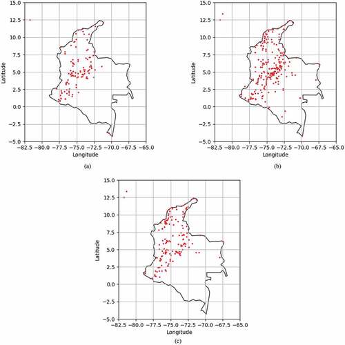
To validate the data available from NSRDB, we used the available in-situ data from IDEAM. Variables GHI, temperature, and wind speed were collected from a total of 116 (Figure 3a), 256 (Figure 3b), and 152 (Figure 3c) stations, respectively, between the years 1998 and 2019. During that time interval, some stations suspended measurements while others started them, so not all the stations had the full data at the complete time interval.

Figure 3. IDEAM in-situ stations spatially located along the Colombian territory collecting data for (a) GHI, (b) temperature and (c) wind speed variables.

Time resolution is also different for each meteorological variable. GHI and wind speed were collected hourly, while three measurements per day were available for temperature stations. The data validation process involved a pre-processing stage for cleaning in-situ data, a time-spatial resolution adjustment, and a bias correction process described as follows.

Clean In-Situ Data. This process consists of removing not-a-number (NaN) values, negative values, and constant values that remained all day (Urraca et al., 2017; Yu et al., 2022). Then, we use an outlier detection process to detect incorrect measurements that the clean data process could omit. Because the climate conditions could change drastically for each station, we analyzed the data per year and per station in the Colombian territory. We used the Local Outlier Factor method, which estimates the local deviation of the density of a given sample for its neighbors (Breunig et al., 2000; Su et al., 2021). We used a total of 30 neighbors samples to analyze each meteorological variable.

Time-Spatial Resolution Adjustment. The spatial resolution of the satellite data is 4 km $\times$ 4 km along the Colombian territory (Sengupta et al., 2018b). In most cases, the spatial location from in-situ data does not match the spatial location of one satellite measurement. Hence, to make satellite and in-situ data comparable, we estimated the variable from satellite, denoted by ${\hat{y}}_i$, for every in-situ station $i$. Sample ${\hat{y}}_i$ is computed as the weighted sum of the four nearest satellite measurements $y_j$ as

(1) $\begin{array}{c}{\hat{y}}_i=\sum _j{w}_{ij}{y}_j,\sum _j{w}_{ij}=1,w_{ij}>0.\end{array}$(1)

Constant $w_{ij}$ scales measurement $y_j$ to compute ${\hat{y}}_i$, defined as

(2) $\begin{array}{c}{w}_{ij}=\frac{1/d_{ij}}{{\sum }_{k}1/d_{ik}},\end{array}$(2)

where $d_{ij}$ is the Euclidean distance between locations $i$ and $j$. Thus, the weighted average of the measurement will be closer to the measurement of the closest locations. Satellite data are reported at a half-hourly time resolution for all meteorological variables. Therefore, for the in-situ data, we take only the satellite measurements at their corresponding time resolution.

Bias Correction. We used Quantile Mapping (QM) to correct the bias in the satellite data using in-situ data. This technique is widely used to transform the distribution function of a modeled variable according to the distribution function of an observed one (Piani et al., 2010; Enayati et al., 2021; Li et al., 2019; Wang et al., 2020), which can be mathematically expressed as

(3) ${\hat{x}}_m=f_o^{-1}[f_m(x_m)],$(3)

where ${\hat{x}}_m$ is the corrected variable, $x_m$ represents the modeled variable, $f_o^{-1}$ is the inverse of the cumulative distribution function (CDF) of the observed variable, and $f_m$ is the CDF of the observed variable.

Validation Metrics. The metrics used in the validation process are the root mean squared error (RMSE), the mean bias error (MBE), and the Pearson correlation coefficient ($\rho$) as shown in Equations (4), (5), and (6):

(4) $RMSE=\sqrt{\frac{1}{N}\sum _{i=1}^N{(x_i-{\hat{y}}_i)}^2},$(4)

(5) $MBE=\frac{1}{N}\sum _{i=1}^N(x_i-{\hat{y}}_i),$(5)

(6) $\rho =\frac{cov(x_i,{\hat{y}}_i)}{{\sigma }_{x_i}{\sigma }_{{\hat{y}}_i}},$(6)

where $x_i$ and ${\hat{y}}_i$ are the in-situ and (pre-processed) satellite measurements. $cov()$ and $\sigma$ refers to the covariance and standard deviation. The RMSE and the MBE allow us to quantify the difference between the satellite and the in-situ data, and $\rho$ allows us to validate if a linear correlation exists between the satellite and the in-situ data. We also computed the relative RMSE (rRMSE)

(7) $rRMSE=\sqrt{\frac{\frac{1}{N}{\sum }_{i=1}^N{(x_i-{\hat{y}}_i)}^2}{{\sum }_{i=1}^N{({\hat{y}}_i)}^2}},$(7)

and the relative MBE (rMBE)

(8) $rMBE=\frac{\frac{1}{N}{\sum }_{i=1}^N(x_i-{\hat{y}}_i)}{{\sum }_{i=1}^N{({\hat{y}}_i)}^2},$(8)

by normalizing the error values with the in-situ data (Urraca et al., 2017; Wang et al., 2016).

Validation Results. Tables 2 and 3 show the validation results before and after the bias correction, respectively. We observe that the Pearson correlation coefficient $\rho$ is still the same after the bias correction. With this result, we make sure that QC only corrects the bias and does not affect the linear distribution of the data. Also, in Figures 4(b), 4(d), and 4(f) we observe how QC corrects the bias of the satellite data and how it is related to the results of the MBE in Tables 2 and 3, where after the bias correction, the MBE and rMBE values for the climate variables drop drastically.

Figure 4. Satellite (x-axis) vs. in-situ (y-axis) averages for GHI (a)(b), temperature (c)(d), and (e)(f) wind speed variables before (left column) and after (right column) bias correction from the period between 1998–2019. Red and green lines represent the 10% and 20% of difference, respectively.

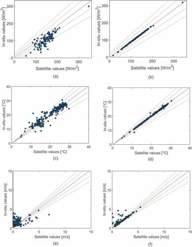
Table 2. Results of the satellite data validation with IDEAM in-situ data before bias correction.

	GHI [W/m^2]	Temperature [°C]	Wind Speed [m/s]
RMSE	116.43 $\pm$ 11.92	2.61 $\pm$ 0.84	1.85 $\pm$ 0.52
%rRMSE	12.07 $\pm$ 1.69	24.01 $\pm$ 14.15	31.95 $\pm$ 15.46
MBE	−25.50 $\pm$ 14.37	0.54 $\pm$ 1.42	0.75 $\pm$ 0.74
%rMBE	−2.72 $\pm$ 1.66	5.72 $\pm$ 17.26	11.93 $\pm$ 19.24
$\rho$	0.91 $\pm$ 0.01	0.75 $\pm$ 0.09	0.31 $\pm$ 0.17

Table 3. Results of the satellite data validation with IDEAM in-situ data after bias correction.

	GHI [W/m^2]	Temperature [°C]	Wind Speed [m/s]
RMSE	105.28 $\pm$ 12.05	2.02 $\pm$ 0.46	1.43 $\pm$ 0.38
%rRMSE	10.84 $\pm$ 1.19	17.96 $\pm$ 6.33	24.08 $\pm$ 6.03
MBE	−0.60 $\pm$ 1.11	−0.02 $\pm$ 0.41	0.21 $\pm$ 0.19
%rMBE	−0.06 $\pm$ 0.12	−0.31 $\pm$ 5.26	2.94 $\pm$ 3.46
$\rho$	0.91 $\pm$ 0.02	0.75 $\pm$ 0.10	0.31 $\pm$ 0.17

The results for $\rho$ show a high linear correlation for GHI and Temperature, with 0.912, and 0.748, respectively. We can also observe that the rRMSE for GHI, temperature, and wind speed, the satellite data are not more different than 11%, 18%, and 24%, with respect to the in-situ data, as shown in Table 3.

3.3. Data visualization

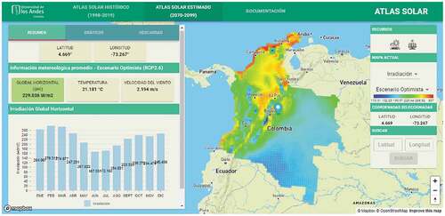
The interactive tool contains three main components: interactive maps, variable graphs, and a photovoltaic generation calculator. In general, a user can select a single point on the map to explore, visualizing a summary of the averages for each variable and several graphs that describe their behavior in the period 1998–2019. Additionally, the user can calculate the PV generation of a system by providing technical information about it. In this subsection, we explain the interactive maps. Each map represents data from a single year and one of five meteorological variables. The photovoltaic generation calculator is explained in Section 5.

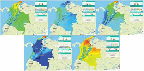
Variable Maps. There is a map for GHI, DHI, DNI, wind speed, and temperature available for each year in the period 1998–2019. Each map contains the yearly averages of all points, representing the value of the selected variable with a color scale (dark blue for the lowest value and red for the highest). The available maps are shown in Figure 5. On the left side of the map, there is a summary of the latitude, longitude, elevation, and yearly averages of the meteorological variables. Inside this panel, the user can access the historical graphs and download the averages for the selected coordinate. The user can change the current map and access the photovoltaic generation calculator on the right side.

Figure 5. Available maps (from left to right and top to bottom): GHI, DHI, DNI, wind Speed, and temperature.

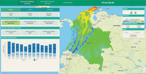
Historical Graphs. We present the historical data on five different graphs depending on the average selected. Each graph can be generated for GHI, DHI, DNI, temperature, and wind speed. Initially, in the general view of the map with historical data (Figure 6), a graph with the global solar irradiance (the sum of the diffuse and direct solar irradiance) for each month of the current year is shown.

Figure 6. General view of the map with historical data.

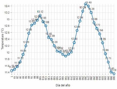
In the Graphs tab, the user can generate the following graphs:

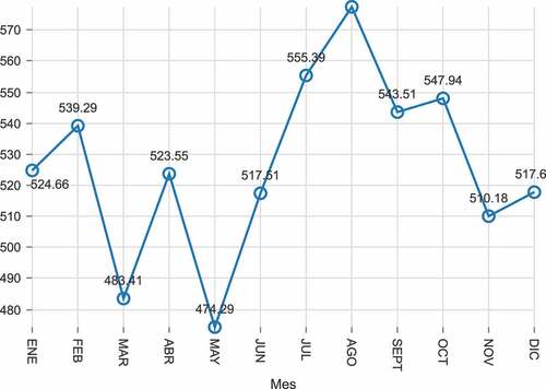
● Monthly Averages: This graph shows the averages per month calculated for a single year. An example can be seen in Figure 7.

Figure 7. Monthly Averages plot.

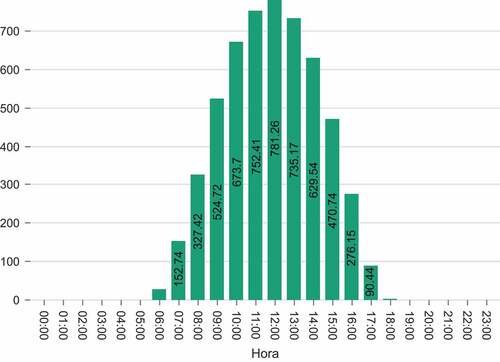
● Hourly Averages: In this case, the graph shows the averages for each hour calculated using the data of a single year. As illustrated in Figure 8, the averages take into account data from every hour, so low values are still shown to the user.

Figure 8. Hourly Averages plot.

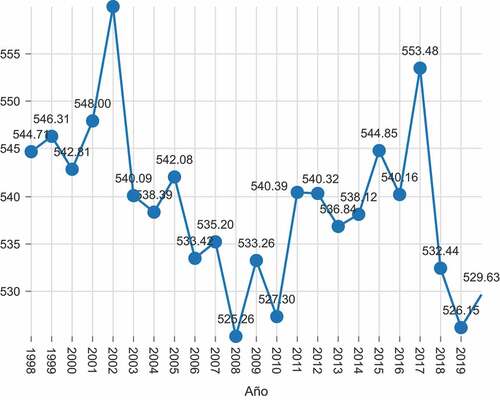
● Historical Yearly Averages: The yearly averages in the period 1998–2019 are shown for a single variable (see Figure 9).

Figure 9. Historical Yearly Averages plot.

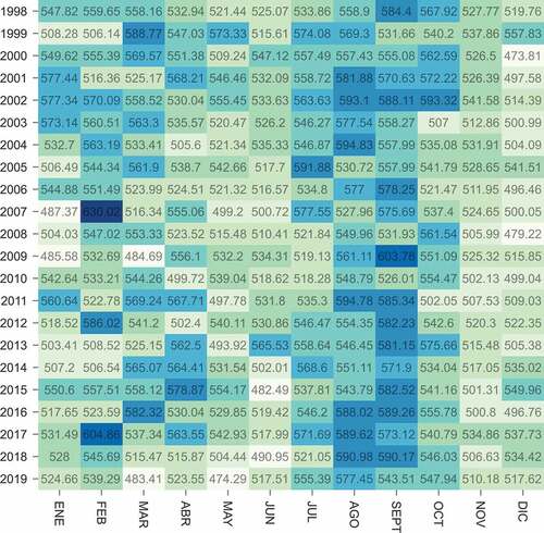
● Historical Monthly Averages: This graph shows the historical data calculated for each month of all years. A heat map with a color gradient is used, where the highest value is shown in dark blue and the lowest in white, as is presented in Figure 10.

Figure 10. Historical Monthly Averages plot.

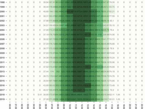
● Historical Hourly Averages: The final graph shows the historical hourly averages per year, using a heat map with a green scale where the shade is assigned depending on the average value, like in Figure 11.

Figure 11. Historical Hourly Average plot.

4. Map with climate change scenarios

4.1. Climate change models

We used the Coordinated Regional Downscaling Experiment (CORDEX) database for the map with climate change scenarios. CORDEX provides high-resolution Regional Climate Model (RCM) projections with great detail (Giorgi et al., 2009). For map purposes, the data include measurements of surface-downwelling shortwave radiation, temperature, and wind speed, with a spatial resolution of 0.2° or 25 km $\times$ 25 km approximately (CORDEX-SAT, 2020). The RCM models are based on representative concentration pathways (RCPs), estimating different greenhouse gas emission scenarios. We show the impact of RCP2.6 (best-case) and RCP8.5 (worst-case) for the different meteorological variables. RCP2.6 scenario corresponds to the case where the increase of the global mean temperature reaches a maximum of 2°C by the end of the century. RCP8.5 scenario corresponds to the case where the increase of the global mean temperature reaches a maximum of 4°C by the end of the century (Van Vuuren et al., 2011; Riahi et al., 2011).

Different studies have demonstrated the accuracy of CORDEX-CORE models in providing consistent and high-resolution regional climate change projections (Giorgi et al., 2021; Teichmann et al., 2021). They state that it is important to understand that these models provide projections, not predictions. These models have also been used to assess the impact of climate change on renewable energies (Zhao et al., 2020; Jerez et al., 2015; Narvaez et al., 2022).

For Colombia, the CORDEX database provides 2,484 coordinates. We downloaded data from 2070 to 2099 for solar irradiance, temperature, and wind speed, for the two RCP scenarios. We worked with this period (2070–2099), intending to have an estimate of the possible PV power potential by the end of the century, and compare this potential with current conditions. Table 4 shows the GCM and RCM models used in this study.

Table 4. An overview of the analyzed CORDEX-CORE experiments. Each experiment has one historical and two scenarios (RCP2.6 and RCP8.5), spanning the periods 1970–2005 and 2070–2099, respectively. The horizontal resolution of all simulations is 0.2° in both latitude and longitude.

	RCM
Forcing GCM run	GERICS-REMO2015	ICTP-RegCM4–7
MOHC-HadGEM2-ES	✓	✓
MPI-M-MPI-ESM-LR	✓
MPI-M-MPI-ESM-MR		✓
NCC-NorESM1-M	✓	✓

4.2. Data visualization

In the same way, a map with historical data was constructed. The map with climate change scenarios contains three main components: interactive maps, graphs of the meteorological variables, and the PV generation calculator. Depending on the two possible RCP, a user can select a single point on the map (a coordinate) to explore, visualizing a summary of the meteorological variables and different plots describing their estimated behavior in 2070–2099. The user can also estimate the PV generation depending on the RCP scenario. The photovoltaic generation calculator is explained in Section 5.

4.2.1. Interactive maps

We developed a map for the meteorological variables (solar irradiance, wind speed, and temperature) available for each proposed scenario, best-case and worst-case. Each map displays an average of the estimated variables between 2070 and 2099 for all points. The available maps are shown in Figure 12.

Figure 12. Available maps (from left to right): solar irradiance, temperature, and wind speed.

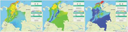
The left side of the map shows a summary with the latitude, longitude, and averages of the variables mentioned above. In the same panel, the user can access the behavior graphs of the variables and download the averages of the variables for a selected coordinate. On the right side of the map, the user can change the current map and access the photovoltaic generation calculator.

4.2.2. Data visualization

The estimated data are presented in two different plots depending on the selected average. Initially, in the general view of the map with estimated data (Figure 13), a graph with the solar irradiance for each month of the selected coordinate is presented.

Figure 13. General view of map with estimated data.

The first graph is the Monthly Behavior, which shows the monthly behavior of the averages of any variable for the selected RCP scenario. Each month is assumed to have 30 days. An example can be seen in Figure 14. The second graph is the Daily Behavior, which shows the daily behavior of the averages of any variable for the selected RCP scenario. The days in the graph are divided into intervals of 10 days, as presented in Figure 15.

Figure 14. Monthly behavior graph.

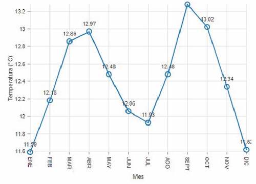
Figure 15. Daily behavior graph.

5. Photovoltaic generation models

The Solar Atlas includes a PV generation calculator for both maps that takes information from an array of solar panels and calculates the power generation per day and month based on two generation models as defined in Molina and Martínez (2017), Boland et al. (2008), De Soto et al. (2006), Dobos (2014), Narvarte and Lorenzo (2008) and Skamarock et al. (2019). Each component of the PV generator calculator is detailed as follows.

5.1. Inclined Radiation

Both models calculate the power generation of the panel array for each day of a given year or a given RCP scenario, depending on the selected map. The first variable defined is the declination angle $\delta$, which is the angle between the equator and a line drawn from the center of the Earth to the center of the sun. $\delta$ varies depending on the position of the Earth relative to the sun and is calculated using the number of the day $d$ and the latitude $\varphi$ as

(9) $\delta ={23.45}^{\circ }sin\left(\frac{360}{365}(284+d)\right).$(9)

The next variable is the solar angle $\alpha$, which measures the angle between the sun’s rays and a horizontal plane, defined as

(10) $\alpha =90-\varphi +\delta .$(10)

The daily averages of GHI for the specific coordinate and year or RCP scenario selected by the user are then used to obtain the inclined radiation $R_i$ as

(11) $Ri=GHI\frac{sin(\alpha +\beta )}{sin(\alpha )},$(11)

where $\beta$ represents the panel array inclination.

5.2. Solar cell temperature

The solar cell temperature $T_c$ is calculated using the panel temperature $T_p$ and the inclined radiation calculated earlier. Initially, $T_p$ is calculated as

(12) $T_p=Ri{exp}^{(a+b\ast WS)}+\mathrm{\Delta }T,$(12)

where $WS$ represents wind speed daily average, $T$ the ambient temperature average, and the constants $a$, $b$, and $\mathrm{\Delta }T$ depend on the type of setup of the array. Both models support two types of setup: isolated (in this case, $a=-3.47$, $b=-0.0594$, and $\mathrm{\Delta }T=3$), or over the roof (where $a=-2.98$, $b=-0.0471$, and $\mathrm{\Delta }T=1$). Therefore, with the panel temperature $T_p$, the solar cell temperature $T_c$ is calculated as

(13) $T_c=T_p+\frac{Ri}{1000}\mathrm{\Delta }T.$(13)

5.3. Nominal power of the system

The nominal power $P_{DCnom}$, in kW, refers to the power produced by the panel array in standard conditions, that is, with global radiation of 1000 W/$m^2$ and a solar cell temperature of 25°C. $P_{DCnom}$ is calculated as

(14) $P_{DCnom}=\frac{P_{mp}N}{1000},$(14)

where $P_{mp}$, in Watts, refers to the maximum panel power, and $N$ refers to the number of panels in the array. These variables are defined by the user.

5.4. Output power – basic generation model

The power produced by the array of panels with the basic generation model $P_{DC}$ is calculated as

(15) $P_{DC}=\frac{Ri}{Rref}{P}_{DCnom}(1+\gamma (T_c-T_0)),$(15)

where $\gamma$ represents the maximum temperature coefficient of the solar cell. This constant is defined by the user. A value of −0.5%/°C is commonly used for monocrystalline solar panel cells. The nominal temperature $T_0$ is 25°C, and the reference radiation $R_{ref}$ is 1000 W/$m^2$.

5.5. Advanced generation model

An advanced generation model is defined based on the I-V curve that describes the behavior of a photovoltaic cell. First, the short circuit current $I_{sc}$ is calculated as

(16) $I_{sc}=I_{sc,ref}\frac{Ri}{1000}(1+\alpha I_{sc}(T_c-T_0)),$(16)

where the reference short circuit current $I_{sc,ref}$, and the short circuit current temperature coefficient $\alpha I_{sc}$, are given by the user depending on the type of solar panel. The short circuit current is then used to calculate the current at maximum power of the panel $I_{mp}$ as

(17) $I_{mp}=I_{mp,ref}\frac{I_{sc}}{I_{sc,ref}},$(17)

where $I_{mp,ref}$ represents the reference current at maximum power given by the user.

The open-circuit voltage $V_{oc}$ is calculated as

(18) $V_{oc}=V_{oc,ref}s\delta (T_c)ln(E_e)+{\beta }_{Voc}(T_c-T_0),$(18)

where the reference open-circuit voltage $V_{oc,ref}$, the number of solar cells in series $s$, and the open-circuit voltage temperature coefficient ${\beta }_{Voc}$ are defined by the user. The constant $\delta (T_c)$ is defined as 26 mV per solar cell.

The open-circuit voltage $V_{oc}$, and the reference voltage at maximum power $V_{mp,ref}$, are then used to calculate the voltage at maximum power of the panel $V_{mp}$ as

(19) $V_{mp}=V_{mp,ref}\frac{V_{oc}}{V_{oc,ref}}.$(19)

Finally, the DC power $P_{DC}$ produced by the solar panel array is calculated using the voltage $V_{mp}$ and current at maximum power $I_{mp}$ as

(20) $P_{DC}=V_{mp}{I}_{mp}.$(20)

5.6. DC/AC inverter and system loss

The DC power $P_{DC}$ calculated using the basic or advanced generation models is converted into AC power as

(21) $P_{AC}=\eta P_{DC},$(21)

where $\eta$ represents the efficiency of the DC/AC inverter. The default value for this constant is 96%, but the user can change it depending on the solar panel.

The calculator takes into account losses produced by dust (2%), shadows (3%), manufacturing defects (2%), wiring (2%), connectors (0.5%), degradation of the cells caused by incident light (1.5%), down time (3%), and discrepancies between theoretical values and the actual performance of the panel (1%), resulting in a total loss $PT$ of 15%. Therefore, the AC power ${\hat{P}}_{AC}$ is defined as

(22) ${\hat{P}}_{AC}=P_{AC}\left(1-\frac{PT}{100}\right).$(22)

5.7. Capacity factor

The capacity factor is the ratio of the annual average energy production and the theoretical maximum annual energy production of a plant assuming it operates at its peak rated capacity every hour of the year (National Renewable Energy Laboratory, 2017). The system rated capacity $SRC$ is calculated as

(23) $SRC=\frac{P_{DCnom}}{DC\mathrm{\_}AC\mathrm{\_}ratio},$(23)

where $P_{DCnom}$ is the nominal power of the system, and $DC\mathrm{\_}AC\mathrm{\_}ratio$ is the relationship between the amount of DC power sent to the AC power inverters; this value is typically 1.25.

Then, the annual energy production $AEP$ is obtained by

(24) $AEP=P_{AC,avg}[kWh]\times 24\left[\frac{hours}{day}\right]\times 365\left[\frac{days}{year}\right]$(24)

where $P_{AC,avg}$ is the average generation based on the daily power values obtained with one of the two generation models.

With the system rated capacity $SRC$ and the annual energy production $AEP$, the capacity factor $CF$ is obtained as

(25) $CF=\frac{AEP[\frac{kWhAC}{year}]}{SRC\times 24[\frac{hours}{day}]\times 365[\frac{days}{year}]}.$(25)

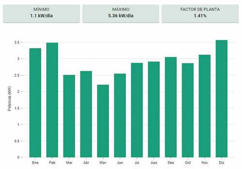
The resulting array of data, consisting of the power produced by the solar panel array for each day in a specific year or RCP scenario, is then used to calculate the average power generation per month, as well as the minimum and maximum power values. The calculator then shows a plot with the calculated values in Figure 16.

Figure 16. Average power generation graph.

6. Conclusion

This paper presents an interactive Solar Atlas that allows users to estimate the PV power potential in Colombia (Colombian Solar Atlas Website). The Solar Atlas has meteorological data from 1998 to 2019 and future projections for 2070–2099. From 1998 to 2019, the database was built using data from the National Solar Radiation Database (NSRDB), a collection of solar and meteorological data with a 4 Km $\times$ 4 Km spatial resolution and a temporal resolution of 30 minutes. With a set of 62,187 points defined for the Colombian territory, we calculated hourly, daily, monthly, and yearly averages of the meteorological variables. From 2070 to 2099, the database includes meteorological data from the CORDEX framework, which provides high-resolution regional climate model (RCM) projections.

As for the data visualization, the averages calculated were represented using a heat map and different types of graphs. For the map with historical data, the heat map shows the yearly averages for a specific year and one of five variables (GHI, DHI, DNI, wind speed, and temperature). The graphs show historical data for a particular point, including daily or monthly averages for a single year. On the other hand, for the map with estimated data, the heat map shows the average for a specific RCP scenario (best-case or worst-case) and one of five variables (GHI, DHI, DNI, wind speed, and temperature). The graphs show the daily or monthly behavior of the averages for any variable at any point.

Additionally, the tool provides two photovoltaic generation models that allow the user to simulate the behavior of a solar panel installation in a specific coordinate and year or RCP scenario, depending on the type of map (historical or estimated). Both models return generation values per day, used to obtain the maximum, minimum, capacity factor, and monthly averages, and visualized with a bar graph.

Finally, this Solar Atlas was made to present the solar photovoltaic potential in Colombia in an interactive and user-friendly way. It also allows the visualization and downloading of meteorological variables that may be of interest to other areas of knowledge. Our interactive tool encompasses all the features of other web atlases, allowing us to change years or visualize different heat maps, and displays them in a user-friendly way. In addition, this tool has a special section for maps related to climate change, which is a feature that no other atlas has.

Acknowledgements

This work was supported by Fundación CEIBA through the program Bécate Nariño, by NVIDIA through the GPU Grant program, and by Centro de Desarrollo Sostenible para América Latina through convocatoria para financiación de proyectos de investigación relacionados con el alcance de los objetivos de desarrollo sostenible. All authors acknowledge the financial support provided by the Vice Presidency for Research and Creation publication fund at the Universidad de Los Andes. We acknowledge the World Climate Research Programme’s Working Group on Regional Climate, and the Working Group on Coupled Modelling, a former coordinating body of CORDEX and responsible panel for CMIP5. We also thank the climate modelling groups (listed in Table 4 of this paper) for producing and making available their model output. Finally, we endorse the National Renewable Energy Laboratory (NREL) for providing the meteorological data.

Disclosure statement

No potential conflict of interest was reported by the authors.

Data availability statement

The data that support the findings of this study are available in the National Solar Radiation Database (NSRDB) at https://developer.nrel.gov/docs/solar/nsrdb/NSRDB, the Coordinated Regional Climate Downscaling Experiment – Coordinated Output for Regional Evaluations (CORDEX-CORE) at https://cordex.org/data-access/how-to-access-the-data/CORDEX-CORE, and the Institute of Hydrology, Meteorology and Environmental Studies (IDEAM) at http://dhime.ideam.gov.co/atencionciudadano/IDEAM.

Supplemental Material

Supplemental data for this article can be accessed online at https://doi.org/10.1080/20964471.2023.2185920.

Additional information

Funding

The work was supported by the Fundación CeiBA, Nvidia, and Centro de Desarrollo Sostenible para América Latina.

Notes on contributors

Gabriel Narvaez

Gabriel Narvaez is currently pursuing doctoral studies in a co-supervision agreement between the Universidad de Los Andes and the University of Toulouse. His lines of research are focused on the management of renewable energies to improve their efficiency and availability through the application of Machine Learning techniques.

Luis Felipe Giraldo

Luis Felipe Giraldo is an Associate Professor of the Department of Biomedical Engineering and a member of the Center for Research and Education in Artificial Intelligence, at Universidad de Los Andes, Colombia. He received a Ph.D. in electrical and computer engineering from the Ohio State University, USA, in 2016. His current research leverages artificial intelligence and technology to address challenges associated with social impact.

Michael Bressan

Michael Bressan is an electrical, electronic, and industrial computing engineer focused on renewable energy systems. He is currently an assistant professor at Universidad de Los Andes, Colombia. He works essentially in energy management and renewable energy, such as photovoltaic systems. He obtained his PhD at the University of Perpignan, France, in June 2014.

Camilo A. Guillen

Camilo Guillen received the Master’s degree in Electronic and Computer Engineering at Universidad de Los Andes, Colombia.

María A. Pabón

María Pabón received a bachelor’s degree in Electronic Engineering at Universidad de Los Andes, Colombia.

Nicolás Díaz

Nicolás Díaz is an Electronic Engineer and a Computer Scientist. He is currently pursuing a master's degree at Universidad de Los Andes, Colombia.

Manuel Felipe Porras

Manuel Porras received a bachelor’s degree in Computer Scientist at Universidad de Los Andes, Colombia.

Brayan Herney Medina

Brayan Medina received a bachelor’s degree in Computer Scientist at Corporación Universitaria del Huila, Colombia.

Fernando Jiménez

Fernando Jiménez is an Associate Professor of the Department of Electrical and Electronic Engineering at Universidad de Los Andes, Colombia. He received a Ph.D. in Computer Systems from Institut National Des Sciences Appliquees De Toulouse.

Guillermo Jiménez-Estévez

Guillermo Jiménez is an electrical engineer from the Escuela Colombiana de Ingeniería Julio Garavito. He holds a master's degree in science and a Ph.D. in electrical engineering from the University of Chile.

Andres Pantoja

Andrés Pantoja is an Associate Professor of the Department of Electronic Engineering at the University of Nariño. He holds an M.Sc. in Electronic and Computer Engineering and Ph.D. in Engineering from Universidad de Los Andes, Colombia.

Corinne Alonso

Corinne Alonso is a full professor of Electrical Engineering at the University of Toulouse Paul Sabatier-Toulouse III. She received her Ph.D. in 1994 in power electronics, INP of Toulouse, and her habilitation to conduct research from the Paul Sabatier University in 2003.

Notes

1. Colombian Solar Atlas Website.

References

- Abril, S. O., León, J. A. P., & Mendoza, J. O. G. (2021). Study of the benefit of solar energy through the management of photovoltaic systems in colombia. International Journal of Energy Economics and Policy, 11, 96. https://doi.org/10.32479/ijeep.10706
- Boland, J., Ridley, B., & Brown, B. (2008). Models of diffuse solar radiation. Renewable Energy, 33, 575–584. https://doi.org/10.1016/j.renene.2007.04.012
- Breunig, M. M., Kriegel, H. P., Ng, R. T., & Sander, J., 2000. Lof: Identifying density-based local outliers, in: Proceedings of the 2000 ACM SIGMOD international conference on Management of data, May 15 - 18, 2000. Dallas Texas, USA. (pp. 93–104). New York, NY, United States: Association for Computing Machinery.
- Chilean Ministry of Energy. (2017). Explorador solar. Retrieved from http://solar.minenergia.cl/exploracion
- CORDEX-SAT, 2020. Regional climate change simulations for cordex domains. URL: https://cordex.org/data-access/regional-climate-change-simulations-for-cordex-domains/.
- De Soto, W., Klein, S. A., & Beckman, W. A. (2006). Improvement and validation of a model for photovoltaic array performance. Solar Energy, 80, 78–88. https://doi.org/10.1016/j.solener.2005.06.010
- Dobos, A. P., 2014. Pvwatts version 5 manual. Technical Report. National Renewable Energy Lab.(NREL), CO (United States).
- Enayati, M., Bozorg-Haddad, O., Bazrafshan, J., Hejabi, S., & Chu, X. (2021). Bias correction capabilities of quantile mapping methods for rainfall and temperature variables. Journal of Water and Climate Change, 12(2), 401–419. https://doi.org/10.2166/wcc.2020.261
- European Comission.2020a. Data sources and calculation methods.
- European Comission.2020b. Pvgis users manual. URL: https://ec.europa.eu/jrc/en/PVGIS/docs/usermanual.
- European Commission Joint Research Centre. (2019). Photovoltaic Geographical Information System. URL. https://re.jrc.ec.europa.eu/pvg_tools/es/
- Gaviria, J. F., Narváez, G., Guillen, C., Giraldo, L. F., & Bressan, M. (2022). Machine learning in photovoltaic systems: A review. Renewable Energy, 196, 298–318. https://doi.org/10.1016/j.renene.2022.06.105
- Gelaro, R., McCarty, W., Suárez, M. J., Todling, R., Molod, A., Takacs, L., Randles, C. A., Darmenov, A., Bosilovich, M. G., Reichle, R., Wargan, K., Coy, L., Cullather, R., Draper, C., Akella, S., Buchard, V., Conaty, A., da Silva, A. M., Gu, W. … Zhao, B. (2017). The modern-era retrospective analysis for research and applications, version 2 (merra-2). Journal of Climate, 30(14), 5419–5454. https://doi.org/10.1175/JCLI-D-16-0758.1
- Giorgi, F., Coppola, E., Jacob, D., Teichmann, C., Abba Omar, S., Ashfaq, M., Ban, N., Bülow, K., Bukovsky, M., & Buntemeyer, L., et al. (2021). The cordex-core exp-I initiative: Description and highlight results from the initial analysis. Bulletin of the American Meteorological Society, 103(2), E293–E310.
- Giorgi, F., Jones, C., & Asrar, G. R. (2009). Addressing climate information needs at the regional level: The cordex framework. World Meteorological Organization (WMO) Bulletin, 58(3), 175.
- Institute of Hydrology, Meteorology and Environmental Studies, 2022. Atlas interactivo. URL: http://atlas.ideam.gov.co/visorAtlasRadiacion.html.
- Jerez, S., Tobin, I., Vautard, R., Montávez, J. P., López-Romero, J. M., Thais, F., Bartok, B., Christensen, O. B., Colette, A., Déqué, M., Nikulin, G., Kotlarski, S., van Meijgaard, E., Teichmann, C., & Wild, M. (2015). The impact of climate change on photovoltaic power generation in europe. Nature Communications, 6(1), 1–8. https://doi.org/10.1038/ncomms10014
- Li, D., Feng, J., Xu, Z., Yin, B., Shi, H., & Qi, J. (2019). Statistical bias correction for simulated wind speeds over cordex-east asia. Earth and Space Science, 6, 200–211. https://doi.org/10.1029/2018EA000493
- Ministerio de Minas y Energía,Unidad de Planeación Minero Energética. ( UPME), 2014. UPME: https://www1.upme.gov.co/Documents/Cartilla_IGE_Incentivos_Tributarios_Ley1715.pdf
- Miranda, E., Fierro, J. F. G., Narváez, G., Giraldo, L. F., & Bressan, M. (2021). Prediction of site-specific solar diffuse horizontal irradiance from two input variables in colombia. Heliyon, 7(12), e08602. https://doi.org/10.1016/j.heliyon.2021.e08602
- Molina, A., Falvey, M., & Rondanelli, R. (2017). A solar radiation database for chile. Scientific Reports, 7, 14823. URL. https://doi.org/10.1038/s41598-017-13761-x.
- Molina, A., & Martínez, F., 2017. Modelo de generación fotovoltaica. URL: http://solar.minenergia.cl/downloads/fotovoltaico.pdf.
- Narvaez, G., Giraldo, L. F., Bressan, M., & Pantoja, A. (2021). Machine learning for site-adaptation and solar radiation forecasting. Renewable Energy, 167, 333–342. https://doi.org/10.1016/j.renene.2020.11.089
- Narvaez, G., Giraldo, L. F., Bressan, M., & Pantoja, A. (2022). The impact of climate change on photovoltaic power potential in southwestern colombia. Heliyon, 8, e11122. https://doi.org/10.1016/j.heliyon.2022.e11122
- Narvarte, L., & Lorenzo, E. (2008). Tracking and ground cover ratio. Progress in Photovoltaics: Research and Applications, 16, 703–714. https://doi.org/10.1002/pip.847
- National Renewable Energy Laboratory, 2017. Solar PV AD-DC Translation. URL: https://atb.nrel.gov/electricity/2017/pv-ac-dc.html.
- National Renewable Energy Laboratory, 2022. NSRDB Data Viewer. URL: https://maps.nrel.gov/nsrdb-viewer/.
- Piani, C., Weedon, G., Best, M., Gomes, S., Viterbo, P., Hagemann, S., & Haerter, J. (2010). Statistical bias correction of global simulated daily precipitation and temperature for the application of hydrological models. Journal of Hydrology, 395(3–4), 199–215. https://doi.org/10.1016/j.jhydrol.2010.10.024
- Riahi, K., Rao, S., Krey, V., Cho, C., Chirkov, V., Fischer, G., Kindermann, G., Nakicenovic, N., & Rafaj, P. (2011). Rcp 8.5—a scenario of comparatively high greenhouse gas emissions. Climatic Change, 109(1–2), 33–57. https://doi.org/10.1007/s10584-011-0149-y
- Sengupta, M., Xie, Y., Lopez, A., Habte, A., Maclaurin, G., & Shelby, J. (2018a). The national solar radiation data base (nsrdb). Renewable and Sustainable Energy Reviews, 89, 51–60. URL https://www.sciencedirect.com/science/article/pii/S136403211830087X
- Sengupta, M., Xie, Y., Lopez, A., Habte, A., Maclaurin, G., & Shelby, J. (2018b). The national solar radiation data base (nsrdb). Renewable and Sustainable Energy Reviews, 89, 51–60. https://doi.org/10.1016/j.rser.2018.03.003
- Skamarock, W. C., Klemp, J. B., Dudhia, J., Gill, D. O., Liu, Z., Berner, J., Wang, W., Powers, J. G., Duda, M. G., & Barker, D. M., et al. (2019). A description of the advanced research wrf model version 4 (Vol. 145). National Center for Atmospheric Research.
- SOLARGIS, 2021. What can you do with solargis? URL: https://solargis.com/docs/getting-started/why-solargis.
- Suri, M., Betak, J., Rosina, K., Chrkavy, D., Suriova, N., Cebecauer, T., Caltik, M., & Erdelyi, B., 2020. Global photovoltaic power potential by country. http://documents.worldbank.org/curated/en/466331592817725242/Global-Photovoltaic-Power-Potential-by-Country.
- Su, X., Wang, L., Zhang, M., Qin, W., & Bilal, M. (2021). A high-precision aerosol retrieval algorithm (hipara) for advanced himawari imager (ahi) data: Development and verification. Remote sensing of environment, 253, 112221.
- Teichmann, C., Jacob, D., Remedio, A. R., Remke, T., Buntemeyer, L., Hoffmann, P., Kriegsmann, A., Lierhammer, L., Bülow, K., Weber, T., Sieck, K., Rechid, D., Langendijk, G. S., Coppola, E., Giorgi, F., Ciarlo`, J. M., Raffaele, F., Giuliani, G., Xuejie, G. … Im, E. -S. (2021). Assessing mean climate change signals in the global cordex-core ensemble. Climate Dynamics, 57(5–6), 1269–1292. https://doi.org/10.1007/s00382-020-05494-x
- Urraca, R., Gracia-Amillo, A. M., Koubli, E., Huld, T., Trentmann, J., Riihelä, A., Lindfors, A. V., Palmer, D., Gottschalg, R., & Antonanzas-Torres, F. (2017). Extensive validation of cm saf surface radiation products over europe. Remote Sensing of Environment, 199, 171–186. https://doi.org/10.1016/j.rse.2017.07.013
- Van Vuuren, D. P., Stehfest, E., den Elzen, M. G., Kram, T., van Vliet, J., Deetman, S., Isaac, M., Goldewijk, K. K., Hof, A., Beltran, A. M., Oostenrijk, R., & van Ruijven, B. (2011). RCP2.6: Exploring the possibility to keep global mean temperature increase below 2°C. Climatic Change, 109(1–2), 95–116. https://doi.org/10.1007/s10584-011-0152-3
- Wang, L., Gueymard, C. A., Bilal, M., Lin, A., Wei, J., Zhang, M., & Yang, X., et al (2020). Constructing a gridded direct normal irradiance dataset in china during 1981–2014. Renewable and Sustainable Energy Reviews, 131, 110004.
- Wang, L., Kisi, O., Zounemat-Kermani, M., Salazar, G. A., Zhu, Z., & Gong, W. (2016). Solar radiation prediction using different techniques: Model evaluation and comparison. Renewable and Sustainable Energy Reviews, 61, 384–397.
- The World Bank, 2017a. Global Solar Atlas. URL: https://globalsolaratlas.info/map.
- The World Bank, 2017b. Global solar atlas - getting started.
- Yu, L., Zhang, M., Wang, L., Qin, W., Jiang, D., & Li, J. (2022). Variability of surface solar radiation under clear skies over Qinghai-Tibet Plateau: Role of aerosols and water vapor. Atmospheric environment, 287, 119286.
- Zhao, X., Huang, G., Lu, C., Zhou, X., & Li, Y. (2020). Impacts of climate change on photovoltaic energy potential: A case study of china. Applied Energy, 280, 115888. https://doi.org/10.1016/j.apenergy.2020.115888