The summer standardized precipitation evapotranspiration index (SPEI) dataset for six European regions over the past millennium reconstructed by tree-ring chronologies

ABSTRACT

Accurate reconstructed series are crucial for studying the differences in regional hydroclimatic variations in Europe over the past millennium. Using hierarchical clustering analysis and stepwise regression methods, we reconstructed yearly time series of the summer standardized precipitation evapotranspiration index (SPEI) for six European regions over the past millennium. Our analysis also revealed prominent regional hydroclimatic differences in multidecadal signals over the past 500 years. For instance, in the 1500s–1570s (from the beginning of the 1500s to the end of the 1570s), drying trends were observed in northern and southeastern Europe, whereas southwestern Europe experienced a wetting trend. Moreover, drying trends were observed in northern and central Europe in the 1640s–1670s. Additionally, wetting trends were observed in western and central Europe during the 1830s–1850s, with drying trends in northern and southeastern Europe. Notably, the hydroclimatic variations in most European regions showed drying trends in the 1920s–1950s, especially in southern Europe. By utilizing large amounts of tree-ring samples and directly comparing regional hydroclimatic variations, our reconstructions provide a consistent and comprehensive dataset for further analysis. The reconstructed dataset is available at https://doi.org/10.57760/sciencedb.07215.

KEYWORDS:

• Europe
• hydroclimatic variations
• regional reconstruction
• tree-ring chronologies
• past millennium

1. Introduction

Tree rings are one of the main proxies indicating past climate changes. Reconstructions over the past hundreds to thousands of years based on tree-ring chronologies are essential for revealing global and regional hydroclimatic variations at decade-century scales (Breitenmoser et al., 2014; Ljungqvist et al., 2020). Due to the broad distributions of trees, many hydroclimate series in European regions have been reconstructed based on tree-ring chronologies (Andreu-Hayles et al., 2017; Cook et al., 2015; Cooper et al., 2013; Dobrovolny et al., 2018; Griggs et al., 2007; Ljungqvist et al., 2019; Martin-Benito et al., 2016; Seftigen et al., 2015a, 2017; Steiger et al., 2018; Wilson et al., 2013). Cook et al. (2015) reconstructed the self-calibrating Palmer drought severity index (scPDSI) in Europe and Mediterranean regions over the past millennium based on chronologies from the International Tree-Ring Data Bank and European tree-ring climatologists, through which the Old-World drought atlas (OWDA) was created. Steiger et al. (2018) developed the Paleo Hydrodynamics Data Assimilation Products (PHYDA) by incorporating reconstructions (including 2,591 tree rings) with model results. Moreover, they found that the European hydroclimate distributions based on the PHYDA were highly correlated with the OWDA. Based on the scPDSI in OWDA, Ljungqvist et al. (2019) revised and expanded the gridded dataset (0.5°×0.5°) for European hydroclimatic variations in the warm season (March–August) during 850–2003 CE (all years hereafter Common Era).

In previous studies, European regional reconstructions based on tree-ring chronologies played indispensable roles in clarifying long-term relationships between hydroclimatic variations and climate drivers. For instance, based on 88 tree-ring widths and 29 maximum latewood density chronologies, the first two principal components of summer hydroclimatic variations in northern Europe over the past millennium were negatively correlated with the North Atlantic Oscillation (NAO) index (Seftigen et al., 2015a). Based on the OWDA, a strong El Niño caused wet (dry) conditions in western (southern) Europe, while it was related to dry conditions in western Europe (King et al., 2020). Moreover, the western Mediterranean hydroclimate was wet during tropical volcanic eruptions and through the following three years. By contrast, hydroclimates in northwestern Europe and the British Isles were dry in response to volcanic eruptions, and the effects are mainly found in years 1–3 following the eruption with the largest moisture deficits in years 2 and 3 (Rao et al., 2017). Additionally, the annually resolved and absolutely dated measurements based on stable carbon and oxygen isotopes of 27,080 tree rings from 21 living and 126 relict oaks (Quercus spp.) were used to reconstruct the summer hydroclimatic variations in central Europe from 75 BCE (Before Common Era) to 2018. The results showed that the sequence of European summer droughts since 2015 was unprecedented over the past 2000 years, probably caused by anthropogenic warming and associated changes in the summer jet stream (Buntgen et al., 2021).

Europe is situated at middle-to-high latitudes, where the land and sea (such as the Atlantic Ocean and the Mediterranean Sea) intersect, resulting in diverse climates and significant regional differences in hydroclimatic variations. For instance, much of western Europe experiences a marine climate, with extratropical cyclone activity and abundant cyclone rainfall. Meanwhile, central and eastern Europe have continental climates, characterized by notable temperature variations and concentrated precipitation. Southern Europe features distinctly Mediterranean climates, with hot and dry summers under the influence of subtropical high-pressure belts and rainy winters influenced by low pressure and strong westerly winds (Eshel & Farrell, 2000; Vautard et al., 2007). Additionally, atmospheric circulation patterns such as the NAO strongly influence hydroclimatic variations across Europe (Hoy et al., 2014). According to Cook et al. (2015), the Medieval Climate Anomaly (MCA) was characterized by dry hydroclimates in most European regions, except for northeastern Europe, parts of Spain, and Ireland. In contrast, the Little Ice Age (LIA) showed a decrease in arid areas compared to the MCA, and wet hydroclimates predominated in most western European regions. In the modern climate period (1850–2012), arid regions continued to decline, and the hydroclimates in most regions, except for eastern Europe, were predominantly wet or not significantly dry.

Clarifying regional differences in hydroclimatic variations over the past millennium is essential for predicting the modern climate under global warming, which also requires reliable reconstructions (Ljungqvist et al., 2016; Steinman et al., 2022). However, direct reconstruction and comparison of existing hydroclimate series in individual European regions has been challenging due to differences in spatial variability, spatiotemporal scales and reconstruction methods (Hofstra & New, 2009; Ljungqvist et al., 2020; Wan et al., 2013). Additionally, the limited and uneven distribution of proxies available for reconstructions of a single area in Europe has further complicated this issue (Ljungqvist et al., 2020). In this respect, we utilized tree-ring chronologies to conduct regional reconstructions based on different periods and obtained hydroclimate series in various European regions over the past millennium. This approach allowed for direct comparison of regional hydroclimatic variations at the same spatiotemporal scales, which is an advantage over previous reconstructions. Furthermore, we made use of as many tree-ring chronologies as possible, including more recent samples, within each European region and during each specific reconstructed period. Therefore, this comprehensive utilization of tree-ring samples enabled us to extract more consistent climate change signals, which highlighted the importance of regional differences in the analysis of past hydroclimatic variations in Europe.

2. Methods

2.1. Study area and data source

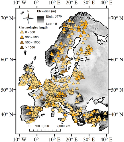
The study area encompassed most European countries, ranging from 32.16°N to 71.68°N in latitude and 10.58°W to 40.93°E in longitude, as shown in Figure 1. Meanwhile, a total of 783 tree-ring sampling sites with 4,746 tree-ring chronologies were included in the analysis, with the majority located in northern and western Europe, the Mediterranean, and Turkey. Nearly 40 tree species were identified, including Picea abies, Quercus spp, Pinus sylvestris, Pinus nigra, and Abies alba. Tree-ring chronologies were obtained from the World Data Service (WDS) for Paleoclimatology Data of the National Oceanic and Atmospheric Administration (NOAA, https://www.ncdc.noaa.gov), with 50 chronologies exceeding 1000 years in length sourced from 14 locations mainly in northern and western Europe. Additionally, 110 chronologies of 500–1000 years and 317 chronologies of 300–500 years were obtained from 45 and 111 locations, respectively, in northern and western Europe, the Mediterranean, and the southern Black Seas. However, only a few chronologies were available from eastern Europe. It is important to note that tree rings in different regions vary in their reliabilities to capture and reconstruct hydroclimate signals due to uncertainties arising from tree species and their surroundings (Babst et al., 2018; Helama et al., 2018; Seftigen et al., 2015a). For instance, in warm and humid areas with frequent human activities, most trees are short-lived, making tree ring growth less sensitive to climatic factors (Gagen et al., 2006; Lavergne et al., 2015; Loader et al., 2008). Furthermore, in regions where multiple climate factors influence tree growth, it is necessary to employ a range of tree ring indicators instead of relying solely on a single index for reconstruction (Gu, 2020; Levesque et al., 2019; Mischel et al., 2015).

Figure 1. Tree-ring chronologies and their length distribution. The topography is derived from NOAA’s global 1 km DEM dataset (https://www.ngdc.noaa.gov/mgg/topo/globe.html) with the WGS 1984 geographic coordinate system and Mercator projected coordinate system. The triangular symbol represents the location of tree-ring chronologies, and the color from light to dark indicates the length from short to long, respectively.

In addition to tree-ring chronologies, monthly precipitation (sums) from the Global Precipitation Climatology Centre (GPCC, https://climatedataguide.ucar.edu/climate-data/gpcc-global-precipitation-climatology-centre) was used for hydroclimate regionalization. To reconstruct hydroclimatic variations over the past millennium, the summer standardized precipitation evapotranspiration index (SPEI) was used. The SPEI has been widely used as a drought index and was designed to measure the difference between precipitation and potential evapotranspiration, reflecting the impact of hydroclimate (Huang et al., 2018; Tao et al., 2014). To calculate the three-month scale SPEI (SPEI–3), gridded precipitation and temperature datasets from the Climatic Research Unit (CRU) TS v.4.03 during 1920–2018 were obtained from the University of East Anglia (https://crudata.uea.ac.uk/cru/data/hrg/) with a spatial resolution of 0.5° × 0.5°. The Penman‒Monteith method, recommended by the Food and Agriculture Organization of the United Nations (FAO) (Begueria et al., 2010, 2014; Vicente-Serrano et al., 2010), was used to obtain the potential evapotranspiration needed for the SPEI calculation. These SPEI values were then used to reconstruct and calibrate hydroclimate series in various European regions.

2.2. Data processing

2.2.1. Hydroclimate regionalization in Europe based on hierarchical clustering analysis (HCA)

In this study, HCA was employed to regionalize hydroclimatic variations in Europe. The HCA has strong statistical characteristics, including its ability to operate without requiring prior assumptions about the data, resilience to the presence of outliers and noise, ease of interpretability and description, and flexibility in distance metrics and linkage methods (Bu et al., 2020; Darand & Mansouri Daneshvar, 2014; Srivastava et al., 2019). It has been widely used in climate regionalization (Abbasi et al., 2022; Han & Zhai, 2015; Qin et al., 2005; Sa’adi et al., 2021). In our study, we used the sum of squared dispersions (SSD) as the criteria for the distance (Han & Zhai, 2015; Ward, 1963), and the specific steps are as follows: (1) treat the hydroclimate series (i.e. precipitation series from GPCC) at each grid point as separate individual regions (Han & Zhai, 2015); (2) calculate the SSD between each pair of sequences, and group the two regions with the smallest SSD into a new region; (3) calculate the average sequence of the new regions as well as the SSD between the regions, and merge the regions with the smallest increase in the SSD; and (4) repeat step (3) until a reasonable number of categories with a sufficiently small (large) SSD in each group (between groups). Moreover, we have taken into account the spatial continuity hypothesis to ensure that our regionalization results align with real-world conditions, implying that similar elements (such as hydroclimate conditions) should not be dispersed across separate partitions (Fang et al., 2017; Zheng et al., 2010).

According to the HCA results (Figure 2), the study area was divided into eight regions with consistent hydroclimatic variations. Notably, although the result reflected hydroclimatic variations, it was actually determined by a combination of direct and indirect factors, including climate type, altitude, topography, and other subsurface conditions. The divided regions included: I. the British Isles region (BRI), II. the Northern Continental region (NCO), III. the Northwestern Coastal region (NWC), IV. the Western Mediterranean region (WME), V. the Eastern Mediterranean region (EME), VI. the Southern Black Sea region (SBS), VII. the Northern Black Sea region (NBS), and VIII. the Eastern Continental region (ECO). It is worth noting that, we implemented minor adjustments during the regionalization to uphold the spatial continuity hypothesis. For instance, we designated the BRI area as a separate region and made further adjustments to incorporate the 15 grid points in the northern part of Scotland, originally classified under the NCO region, within the complete BRI region. Furthermore, our regionalization was refined based on insights from previous studies, allowing us to uncover the key characteristics of regional discrepancies in hydroclimatic variations across Europe. We identified that approximately 20 grid points in the southeastern part of the WME were classified within the EME during the initial HCA result. To improve this inconsistency with the climate types defined in the updated Köppen classifications (Kottek et al., 2006; Peel et al., 2007), we made necessary adjustments to reclassify these grid points as belonging to the WME. On the other hand, the tree-ring distribution was considered to ensure that enough chronologies were significantly correlated with the regional hydroclimatic variations. In our study, since only a few chronologies were located in the NBS and ECO (Figure 1), subsequent reconstructions were not performed in these two regions.

Figure 2. Regionalization of European hydroclimatic variations based on HCA, with spatial distribution of summer precipitation in Europe (blue shadows) and region-specific variations in summer precipitation (small figures), sourced from GPCC.

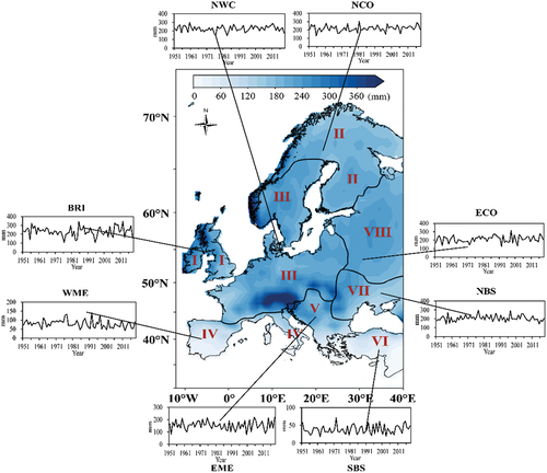
As shown in Figure 2, the summer precipitation in the WME, EME, and SBS was relatively lower than that in the BRI, NCO, and NWC. This difference may be attributed to the asynchronous changes in precipitation and heat resulting from the Mediterranean climate (Deitch et al., 2017). The BRI experienced a general increase in precipitation after the 1980s, while the fluctuations in precipitation were smaller in NWC and NCO than in the BRI. In the NWC, there was an increase in precipitation during 1980–2010. In the WME, although there was abundant precipitation in 1991 and 1997, there was a significant decrease after the 1980s. Moreover, the SBS had the lowest precipitation throughout the period, mainly due to the influence of subtropical high pressure, but showed an increasing trend after 2010.

2.2.2. Regional reconstruction of European hydroclimatic variations over the past millennium

According to our regionalization, stepwise regression analysis (SRA) was used to select tree-ring chronologies contributing to the variance in regional hydroclimatic variations. Then, the partial least squares regression (PLSR) was further used to build calibration models to avoid redundant errors from high correlations between regional chronologies. In addition, we used the leave-one-out cross-validation to calculate the root-mean-square error (RMSE) of the regression model and to verify the model’s validity (Gong et al., 2007). For the calibration and verification periods, $\mathit{RMSE}$ is defined as $\mathit{RMSEC}$ and $\mathit{RMSEV}$, respectively.

Since the number of regional tree-ring chronologies available for calibration differed in various periods, the period-based method was employed to maximize the use of chronologies and to reconstruct a series as long as possible (Fritts, 1972). To be more specific, we split the reconstructed periods according to the start and end years of each available tree-ring chronology. Subsequently, we selected chronologies that encompassed these diverse periods and demonstrated significant correlation (p < 0.1) with the SPEI during the calibration periods. Calibration equations were then developed utilizing these selected chronologies, employing the SRA and PLSR (p < 0.05 for the F-test). Additionally, we incorporated the corresponding SPEI series calculated from observations during the calibration period into the calibration process. Taking reconstructions in the BRI as an example (Table 1), among 305 regional tree-ring chronologies, there were 107 chronologies significantly correlated with the summer SPEI in calibrated periods. Before 1649, the predicted variance explanation ($R_{\mathit{pr}}^2$) of the calibrated model was less than 20% and the series was not reconstructed. In 1649–1659, two chronologies contributing to SPEI variances were selected by the SRA, and the $R_{\mathit{pr}}^2$ of the calibration model based on the PLSR was 21%. In 1885–1976, the number of candidate chronologies increased to 107, and five chronologies were selected for the reconstruction. In 1998–2003, the number of candidate chronologies decreased to 7, and two chronologies contributed to regional hydroclimatic variations. Moreover, the $R_{\mathit{pr}}^2$ was 24%, and the series was reconstructed. However, the $R_{\mathit{pr}}^2$ was less than 20% after 2003, and the reconstruction was stopped. Notably, due to differences in calibration model variances during various periods, it is necessary to perform the variance matching method based on regional SPEI variances. Finally, we obtained a series of summer hydroclimatic variations in the BRI with consistent variance.

Table 1. The period, calibration model, number of chronologies, and some evaluation parameters used for reconstructions in the BRI.

Period	Calibration model	${\mathit{R}}_{\mathit{pr}}^2$	Sample number	1920–1976
				$\mathit{RMSEC}$	$\mathit{RMSEV}$
1649–1659	0.124–0.274 × BRI070rs + 0.198 × BRI071rs 0.124 + 0.226 × BRI064rs − 0.283 × BRI070rs	0.21	2	0.682	0.729
1660–1701		0.24	3	0.672	0.713
1702–1704	0.124 + 0.226 × BRI064rs − 0.283 × BRI070rs 0.127–0.200 × BRI026rr − 0.271 × BRI026xa + 0.228 × BRI071rs 0.130 + 0.201 × BRI015ls − 0.659 × BRI015xr − 0.146 × BRI026er + 0.175 × BRI064rs 0.130 + 0.201 × BRI015ls − 0.659 × BRI015xr − 0.146 × BRI026er + 0.175 × BRI064rs 0.130 + 0.201 × BRI015ls − 0.659 × BRI015xr − 0.146 × BRI026er + 0.175 × BRI064rs 0.130 + 0.201 × BRI015ls − 0.659 × BRI015xr − 0.146 × BRI026er + 0.175 × BRI064rs 0.130 + 0.201 × BRI015ls − 0.659 × BRI015xr − 0.146 × BRI026er + 0.175 × BRI064rs 0.130 + 0.201 × BRI015ls − 0.659 × BRI015xr − 0.146 × BRI026er + 0.175 × BRI064rs	0.24	4	0.672	0.713
1705–1720		0.34	15	0.615	0.664
1721–1728		0.56	22	0.485	0.541
1729–1765		0.56	26	0.485	0.541
1766–1783		0.56	36	0.485	0.541
1784–1784		0.56	48	0.485	0.541
1785–1792		0.56	49	0.485	0.541
1793–1802		0.56	50	0.485	0.541
1803–1807	0.130 + 0.201 × BRI015ls − 0.659 × BRI015xr − 0.146 × BRI026er + 0.175 × BRI064rs 0.130 + 0.201 × BRI015ls − 0.659 × BRI015xr − 0.146 × BRI026er + 0.175 × BRI064rs 0.130 + 0.201 × BRI015ls − 0.659 × BRI015xr − 0.146 × BRI026er + 0.175 × BRI064rs 0.130 + 0.201 × BRI015ls − 0.659 × BRI015xr − 0.146 × BRI026er + 0.175 × BRI064rs 0.130 + 0.201 × BRI015ls − 0.659 × BRI015xr − 0.146 × BRI026er + 0.175 × BRI064rs	0.56	51	0.485	0.541
1808–1822		0.56	58	0.485	0.541
1823–1836		0.56	61	0.485	0.541
1837–1838		0.56	68	0.485	0.541
1839–1845		0.56	69	0.485	0.541
1846–1846	0.130 + 0.201 × BRI015ls − 0.659 × BRI015xr − 0.146 × BRI026er + 0.175 × BRI064rs	0.56	72	0.485	0.541
1847–1847	0.136 + 0.251 × BRI004rs − 0.683 × BRI015xr + 0.273 × BRI024xr − 0.311 × BRI027rs + 0.172 × BRI064rs	0.65	73	0.425	0.485
1848–1852	0.136 + 0.251 × BRI004rs − 0.683 × BRI015xr + 0.273 × BRI024xr − 0.311 × BRI027rs + 0.172 × BRI064rs	0.65	74	0.425	0.485
1853–1855	0.136 + 0.251 × BRI004rs − 0.683 × BRI015xr + 0.273 × BRI024xr − 0.311 × BRI027rs + 0.172 × BRI064rs	0.65	75	0.425	0.485
1856–1856	0.136 + 0.251 × BRI004rs − 0.683 × BRI015xr + 0.273 × BRI024xr − 0.311 × BRI027rs + 0.172 × BRI064rs	0.65	77	0.425	0.485
1857–1859	0.136 + 0.251 × BRI004rs − 0.683 × BRI015xr + 0.273 × BRI024xr − 0.311 × BRI027rs + 0.172 × BRI064rs	0.65	78	0.425	0.485
1860–1860	0.136 + 0.251 × BRI004rs − 0.683 × BRI015xr + 0.273 × BRI024xr − 0.311 × BRI027rs + 0.172 × BRI064rs	0.65	84	0.425	0.485
1861–1873	0.136 + 0.251 × BRI004rs − 0.683 × BRI015xr + 0.273 × BRI024xr − 0.311 × BRI027rs + 0.172 × BRI064rs	0.65	88	0.425	0.485
1874–1877	0.136 + 0.251 × BRI004rs − 0.683 × BRI015xr + 0.273 × BRI024xr − 0.311 × BRI027rs + 0.172 × BRI064rs	0.65	89	0.425	0.485
1878–1878	0.136 + 0.251 × BRI004rs − 0.683 × BRI015xr + 0.273 × BRI024xr − 0.311 × BRI027rs + 0.172 × BRI064rs	0.65	94	0.425	0.485
1879–1884	0.136 + 0.251 × BRI004rs − 0.683 × BRI015xr + 0.273 × BRI024xr − 0.311 × BRI027rs + 0.172 × BRI064rs	0.65	95	0.425	0.485
1885–1976	0.136 + 0.251 × BRI004rs − 0.683 × BRI015xr + 0.273 × BRI024xr − 0.311 × BRI027rs + 0.172 × BRI064rs	0.65	107	0.425	0.485
1977–1978	0.134–0.457 × BRI017xa − 0.231 × BRI027rs + 0.171 × BRI040rs + 0.222 × BRI064rs	0.58	59	0.480	0.528
1979–1979	0.129–0.247 × BRI027rs + 0.255 × BRI064rs − 0.237 × BRI070rs	0.29	13	0.630	0.684
1980–1984	0.129–0.247 × BRI027rs + 0.255 × BRI064rs − 0.237 × BRI070rs	0.29	11	0.630	0.684
1985–1988	0.129–0.247 × BRI027rs + 0.255 × BRI064rs − 0.237 × BRI070rs	0.29	9	0.630	0.684
1989–1997	0.124 + 0.226 × BRI064rs − 0.283 × BRI070rs	0.24	8	0.672	0.706
1998–2003	0.124 + 0.226 × BRI064rs − 0.283 × BRI070rs	0.24	7	0.672	0.706

Note: the variable naming convention follows the format of “region abbreviation of the tree-ring sample + site number + type of tree-ring index + type of chronology”. The tree-ring indexes used in the model include total ring density (d), earlywood width (e), earlywood density (i), latewood width (l), minimum density (n), ring width (r), latewood density (t), maximum density (x), and latewood percent (p). The available chronology types include ARSTND (a), low pass filter (p), residual (r), standard (s), and re-whitened residual (w). The “sample number” indicates the total number of tree-ring chronologies used in the calibration model for each time period.

In addition, the series in other five European regions were also reconstructed according to the method mentioned above. Table 2 provides a concise overview of the complete reconstruction periods, typical tree-ring chronologies utilized for calibration models, and various evaluation parameters for the remaining five European regions. Detailed information on these regions can be also found in Tables S1–S5.

Table 2. Brief information for reconstructions in the other five European regions. “Max” and “Min” refer to the maximum and minimum value of the parameters for each period, respectively.

Region	Complete period	Typical tree-ring chronologies in calibration model	Max ${\mathit{R}}_{\mathit{pr}}^2$	Max sample number	Min RMSEC	Min RMSEV
NCO	517–2006	FINL018xa, SWED0330xs, NORW003na, etc.	0.67	137	0.311	0.386
NWC	1623–2010	GERM052xs, SWIT112xa, AUST008ns, etc.	0.84	426	0.148	0.203
WME	1515–2008	FRAN043xs, SPAI069xs, ITAL016rs, etc.	0.78	214	0.226	0.273
EME	1647–2008	GREE005xa, BULG003xs, YUGO004rs, etc.	0.64	92	0.403	0.471
SBS	1455–2004	TURK014rs, TURK052rs, CYPR009rs, etc.	0.67	195	0.338	0.410

3. Results

3.1. Hydroclimate reconstructions in six European regions over the past millennium

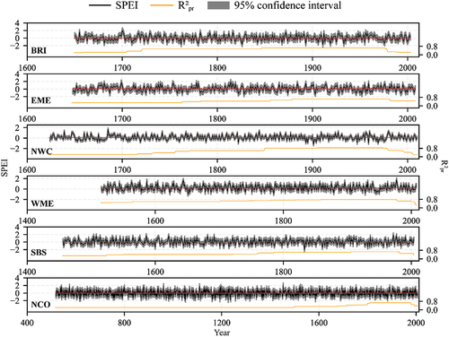
Figure 3 shows the reconstructions in six European regions. Among the six regional reconstructed series in Europe, the longest was in the NCO with 1490 years (517–2006). Moreover, the highest $R_{\mathit{pr}}^2$ (0.67) was in 1810–1978, and the lowest one (0.22) was in 517–1499. In the BRI, the reconstructed period was 1649–2003 (355 years), with the highest $R_{\mathit{pr}}^2$ (0.65) in 1847–1976 and the lowest (0.21) in 1649–1659. In the NWC, reconstructions spanned 1623–2010 (388 years), with the highest $R_{\mathit{pr}}^2$ (0.84) in 1905–1974 and the lowest (0.21) in 1623–1715. In the WME, the reconstructed period was 1515–2008 (494 years), with the highest $R_{\mathit{pr}}^2$ (0.78) in 1859–1977 and the lowest (0.22) in 2008. In the EME, the reconstructed period was 1647–2008 (362 years), with the highest $R_{\mathit{pr}}^2$ (0.64) in 1879–1981 and the lowest (0.29) in 1647–1762. In the SBS, the reconstruction spanned 1455–2004 (550 years), with the highest $R_{\mathit{pr}}^2$ in 1906–1978 (0.67) and the lowest (0.29) in 1455–1523.

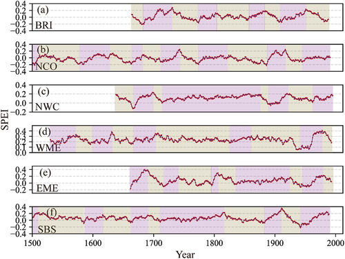
Figure 3. Reconstructed hydroclimatic variations in six European regions.

3.2. Differences in European regional hydroclimatic variations over the past 500 years

Figures 4 and 5 show the decadal (11-year sliding averages) and multidecadal (31-year sliding averages) signals extracted from six European regional reconstructions. In general, decadal hydroclimatic variations in most regions were more distinct before the 1750s and after the 1850s. However, there were also differences in specific periods (Figure 4). For instance, in the BRI (Figure 4(a)), prominent drying trends of the hydroclimate existed in the 1660s–1680s (from the beginning of the 1660s to the end of the 1680s), the 1700s, the 1720s–1750s, the 1890s–1910s, the 1930s, and the 1960s–1970s, while prominent wetting trends occurred during periods such as the 1690s–1700s, the 1710s, the 1850s–1880s, the 1940s–1960s, and the 1970s–1990s. In the NCO (Figure 4(b)), drying trends occurred during periods such as the 1530s–1580s, the 1640s–1650s, the 1750s–1760s, the 1860s–1870s, and the 1900s–1930s, while wetting trends occurred during periods such as the 1510s–1520s, the 1590s–1600s, the 1710s–1740s, the 1880s–1900s, the 1940s–1960s, and the 1970s–1990s. In the NWC (Figure 4(c)), drying trends existed during periods such as the 1630s–1670s, the 1690s–1700s, the 1960s, and the 1980s–2000s, while wetting trends occurred during periods such as the 1680s, the 1900s–1920s, and the 1970s.

Figure 4. The 11-year sliding averages of the reconstructed hydroclimate series in six European regions over the past 500 years. Brown shading indicates a decreasing trend, while red shading indicates an increasing trend in the series during the specified period.

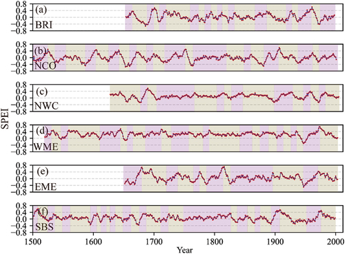
Figure 5. The 31-year sliding averages of the reconstructed hydroclimate series in six European regions over the past 500 years. Brown shading indicates a decreasing trend, while red shading indicates an increasing trend in the series during the specified period.

In the WME (Figure 4(d)), dry trends occurred in periods such as the 1530s–1540s, the 1640s–1650s, the 1910s–1940s, and the 1970s–1990s, while wetting trends occurred in periods such as the 1550s–1560s, the 1610s–1640s, and the 1950s–1970s. In the EME (Figure 4(e)), dry trends occurred during periods such as the 1680s–1710s, the 1740s–1760s, the 1780s, the 1810s–1820s, and the 1970s–2000s, while the wetting trend occurred in periods such as the 1650s–1670s, the 1720s–1730s, the 1760s–1770s, the 1790s–1810s, and the 1950s–1970s. In the SBS (Figure 4(f)), dry trends occurred in periods such as the 1510s–1520s, the 1660s–1670s, the 1910s–1930s, and the 1970s–1990s, while the wetting trend occurred in periods such as the 1500s, the 1600s, the 1670s, the 1890s–1900s, and the 1950s–1970s.

The multidecadal hydroclimatic variations were consistent with the decadal variations (Figure 5). For instance, in the BRI (Figure 5(a)), drying trends of the hydroclimate occurred during periods such as the 1660s–1680s, the 1730s–1770s, the 1880s–1900s, and the 1950s–1980s, while wetting trends occurred during periods such as the 1680s–1730s, the 1770s–1800s, the 1850s–1880s, and the 1900s–1950s. In the NCO (Figure 5(b)), drying trends occurred in periods such as the 1520s–1580s, the 1630s–1660s, the 1740s–1770s, the 1830s–1880s, and the 1910s–1930s, while wetting trends occurred in periods such as the 1580s–1630s, the 1710s–1740s, the 1770s–1810s, and the 1880s–1910s. In the NWC (Figure 5(c)), drying trends occurred in periods such as the 1640s–1660s, the 1700s–1710s and the 1920s–1960s, while wetting trends occurred in periods such as the 1660s–1700s, the 1710s–1870s, the 1880s–1920s, and the 1960s–1990s.

In the WME (Figure 5(d)), drying trends occurred during periods such as the 1570s–1590s, the 1630s–1660s, the 1700s–1830s, the 1870s–1940s, and the 1980s–1990s, while wetting trends occurred during periods such as the 1530s–1570s, the 1660s–1700s, and the 1950s–1980s. In the EME (Figure 5(e)), drying trends occurred in periods such as the 1690s–1710s, the 1810s–1830s, the 1930s–1950s, and the 1980s–1990s, while wetting trends occurred in periods such as the 1660s–1690s, the 1710s–1740s, the 1800s, and the 1950s–1980s. In the SBS (Figure 5(f)), drying trends occurred in periods such as the 1510s–1580s, the 1810s–1870s, and the 1910s–1950s, while wetting trends occurred in periods such as the 1580s–1610s, the 1660s–1690s, the 1880s–1910s, and the 1950s–1980s.

Meanwhile, comparing the multidecadal hydroclimatic variations in Europe, significant regional differences could be found (Figure 5). For instance, during the 1500s–1570s, there were drying trends in northern and southeastern Europe (NCO and SBS), and a wetting trend in southwestern Europe (WME), which may be attributed to the NAO’s contributions (Rodrigo et al., 2000). During the 1640s–1670s, there were drying trends in northern and central Europe (NCO and NWC), which was consistent with some Swedish summer droughts reconstructed by documentary evidence (Leijonhufvud & Resto, 2021). During the 1670s–1700s, hydroclimates in most European regions showed wetting trends, especially in central and southern Europe (NWC, WME, and EME). However, there was a drying trend in part of western Europe (BRI). During the 1700s–1800s, hydroclimates in western and northern Europe (BRI and NCO) showed wetting trends until the 1740s and then turned into dry trends. Meanwhile, hydroclimates in southeastern and central Europe (SBS and NWC) showed a wet trend. During the 1810s–1830s, hydroclimates in southeastern Europe (EME and SBS) transitioned from relative wetness to dryness. A relevant study suggested hydroclimatic variations in eastern Mediterranean regions were probably consistent with a persistent NAO mode (Benito et al., 2015).

During the 1830s–1850s, hydroclimates showed wetting trends in western and central Europe (NWC and WME), while drying trends occurred in northern and southeastern Europe (NCO and SBS). During the 1880s–1910s, hydroclimates in part of western Europe (BRI) switched from relative wetness to dryness, while the variations in northern, central, and southeastern Europe (NCO, NWC, and SBS) were reversed, probably triggered by the summer NAO (Rocha et al., 2020). During the 1920s–1950s, hydroclimates in most regions (except for the BRI) showed drying trends, especially in southern Europe (WME, EME, and SBS). After the 1950s, hydroclimates in southern Europe (WME, EME, and SBS) switched from relative dryness to wetness, while variations in part of western Europe (BRI) were reversed, consistent with previous reconstructions (Loader et al., 2020; Rinne et al., 2013).

4. Validation and discussion

4.1. Quality control of the dataset

In this study, we employed strict quality control in the reconstruction process through data source selection and statistical analysis. For instance, only tree-ring chronologies significantly correlated with hydroclimatic variations were selected for reconstruction. Therefore, chronologies with less contribution to the variance of hydroclimatic variations were eliminated, ensuring more effective indicators of chronologies in regional reconstructions. For calibration models, we also performed strict statistical tests on each process according to the requirements of paleoclimatic reconstruction, including the F test for the SRA and PLSR.

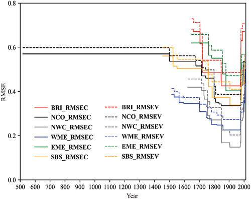
Figure 6 shows the $\mathit{RMSEC}$ and $\mathit{RMSEV}$ of reconstructions in six European regions. For the BRI series, the lowest values of $\mathit{RMSEC}$ and $\mathit{RMSEV}$ in each reconstructed period were 0.425 and 0.485, respectively. For the NCO, the lowest values were 0.336 and 0.386, respectively. For the NWC, the lowest values were 0.148 and 0.203, respectively. For the WME, the lowest values were 0.226 and 0.273, respectively. For the EME, the lowest values were 0.403 and 0.467, respectively. For the SBS, the lowest values were 0.338 and 0.410, respectively. In general, although reconstructions of the NWC and WME performed relatively well, all of the regional reconstructions in Europe may turn out to be reliable.

Figure 6. The $\mathit{RMSEC}$ and $\mathit{RMSEV}$ of hydroclimatic variations in various European regions.

4.2. Comparison with previous studies

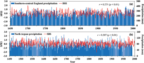
Figure 7 compares our reconstructions with previously reconstructed precipitation series. There was a significant ($1650-2013,\mathit{r}=0.271,\mathit{p}<0.01$) correlation between the series in the BRI and the March-July precipitation in south-central England reconstructed by the well replicated oak ring-width composite chronologies using living and historical material (Wilson et al., 2013), especially during the 1700s–1800s and the 1850s–2000s (Figure 7(a)). In comparison to the living tree-ring chronology samples utilized for constructing our final calibration equations in BRI (BRI004, BRI015, BRI017, BRI026, BRI027, BRI040, BRI064, BRI070, and BRI071 in WDS), we found that only BRI004 and BRI064 overlapped with the south-central England series, and the shared samples accounted for a very small portion relative to the total samples used in each study. Meanwhile, there was a significant ($1455-1989,\mathit{r}=0.307,\mathit{p}<0.01$) correlation between the SBS series and precipitation in the northern Aegean Sea region, especially during the 1500s–1600s, the 1700s–1780s, and the 1800s–1970s (Figure 7(b)). In comparison to the samples used in constructing calibration equations in SBS (TURK008, TURK014, TURK017, TURK028, CYPR005, CYPR009, CYPR012, CYPR019, etc.), the reconstruction in the northern Aegean Sea region utilized distinct tree ring samples. These included seven modern forest chronologies from Chalkidiki, Livadia, Istanbul, and Bursa, along with 49 historic building chronologies (Griggs et al., 2007).

Figure 7. Comparison of reconstructed series in the BRI, WME, and SBS with previously reconstructed precipitation series from European regions, including (a) March-July precipitation (sums) in south-central England during 1650–2003 (Wilson et al., 2013) and (b) may-June precipitation (sums) in the northern Aegean region during 1450–1989 (Griggs et al., 2007).

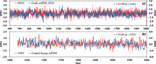
Figure 8 compares our reconstructions with some previously reconstructed hydroclimate indicators. The NCO series and summer scPDSI of OWDA with the same NCO domain were significantly ($601-2006,\mathit{r}=0.199,\mathit{p}<0.01$) correlated, particularly during the 700s–1400s, the 1600s–1700s, and the 1900s–2000s (Figure 8(a)). Moreover, there was also a significant ($1623-2000,\mathit{r}=0.143,\mathit{p}<0.01$) correlation between the NWC series and the summer scPDSI in central Europe, especially during the 1700s–1950s (Figure 8(b)). In comparison to the samples used in constructing calibration equations in NWC (SWIT105, SWIT112, SWIT115, GERM047, GERM048, GERM051, AUST008, CZEC001, CZEC003, etc.), the samples employed for the summer scPDSI in central Europe relied on tree-ring stable isotopes, specifically delta 13C and delta 18O (Buntgen et al., 2021). Overall, our reconstructions maintained consistent variations with existing reconstructed precipitation or other hydroclimate indicators, suggesting their considerable reliability in capturing the characteristics of hydroclimatic variations over the past millennium.

Figure 8. Comparison of reconstructions in the NCO and NWC with the previous reconstructed hydroclimate indicators in European regions, including (a) summer scPDSI of OWDA in the same NCO domain during 600–2006 (Cook et al., 2015), and (b) summer scPDSI in central Europe during 1623–2000 (Buntgen et al., 2021).

It is noteworthy that our study utilized a significantly large number of tree-ring chronologies for each European region in the reconstruction. To assess the reliability of the hydroclimate information in our reconstructions, we conducted a comparison with some European sub-regional series in previous studies. The relatively high correlation coefficients indicated the capacity of our reconstructions to reveal and integrate regional hydroclimate signals effectively. However, we recognized the potential risk associated with correlating our series with previous studies that use the same tree-ring samples. To address this concern, we compared our series with previous ones that utilize less same tree-ring samples. For instance, in the case of our final calibration equations in the BRI series, we incorporated tree-ring samples from multiple sites, with only two sites overlapping with the south-central England reconstruction. It is important to note that the south-central England reconstruction also utilized various tree-ring samples from other sites, including some historical material. Furthermore, in our SBS and NWC series, the tree-ring samples in the calibration equations differed from those employed in the northern Aegean region and central Europe reconstructions. Therefore, comparing our results with previous studies can be useful in evaluating the extent to which we have captured hydroclimatic variation in various regions across Europe.

4.3. Possible uncertainties of the dataset

Although many methods were employed to ensure the reliability of our reconstructions, some factors still introduced uncertainty. During some sub-periods, there were differences between our series and previous reconstructions. For instance, BRI hydroclimatic variations were inconsistent with south-central England precipitation during the 1650s–1700s (Figure 7(a)). Moreover, the variations in SBS hydroclimate differed from the precipitation in northern Aegean during the 1600s–1700s (Figure 7(b)). These differences may be attributed to the domains and seasonality of reconstructions or some mixed signals of temperature and humidity contained in the tree rings (Dannenberg & Wise, 2016; Liu et al., 2021).

On the other hand, there were also differences between our reconstructions and other previous reconstructed hydroclimate indicators. For instance, the NCO hydroclimatic variations were inconsistent with the summer scPDSI of OWDA in the same NCO domain during some subperiods, such as the 1400s–1600s and the 1700s–1800s (Figure 8(a)). Furthermore, differences existed between the NWC’s hydroclimate and the summer scPDSI in central Europe during the 1600s–1700s (Figure 8(b)). The observed differences can be attributed to variations in the reconstructed regions, such as the NWC area and central Europe, as well as the utilization of diverse hydroclimate indicators for calibration (Li et al., 2015; Zhang et al., 2016). Notably, the discrepancies between scPDSI and SPEI in elucidating European hydroclimatic variations are of particular importance (Cook et al., 2014; Trnka et al., 2016). Moreover, there were also some uncertainties in the SPEI for calibration in our reconstruction due to selections of the input data, observation periods, and evapotranspiration models (Hoffmann et al., 2020; Laimighofer & Laaha, 2022; Shi et al., 2020).

Meanwhile, the length and distribution of tree-ring chronologies from different European regions used in reconstruction also contributed to the uncertainties in our study, which fall under the spatiotemporal bias of data. In fact, we have taken this into account by selecting six European regions for reconstruction. It was important to note that the impact of this spatiotemporal bias was significant in the variation of $R_{\mathit{pr}}^2$ values, even for the same series during different time periods, caused by the differences in the lengths and locations of tree-ring samples. For instance, an increased number of valid tree-ring samples from a region during specific periods could lead to smaller uncertainties in the hydroclimate reconstructions, while a smaller number of valid samples could result in greater uncertainties.

Notably, we made some minor adjustments during the regionalization process, guided by the spatial continuity hypothesis. These adjustments were aimed at concentrating sub-regions with similar hydroclimate conditions, although they may introduce some uncertainties in accurately reflecting the identified hydroclimatic commonalities. Moreover, apart from the spatial continuity hypothesis, it is important to consider other factors that contribute to the rationale behind these adjustments, which should be explored in future research. For instance, the need to switch 15 grid points from the NCO to BRI may also be driven by the varying influence of growing season temperature on tree growth between the NCO region and northern Scotland (Makinen et al., 2003; Nojd et al., 2017; Stridbeck et al., 2022).

Despite drawing on certain aspects of regionalization from previous research, our regionalization diverged significantly from previous results. Rather than mainly relying on climate types with relatively coarse categorizations, our emphasis lies in capturing hydroclimatic variations. This shift in focus allows for a more detailed division, which in turn facilitates the comprehensive reconstruction of hydroclimate series spanning the past millennium in Europe. However, it is important to recognize that further research is still needed to fully comprehend the limitations of our reconstructed method. Additionally, exploring alternative regionalization methods may provide more representative references for the underlying hydroclimate dataset.

5. Usage notes

Our reconstructed dataset provides the hydroclimatic variation series in six European regions. The file of our dataset contains ten columns, including the reconstructed year (year), reconstructed SPEI value (value), ±95% confidence interval for the uncertainty range (−95% and 95%), mean value over the reconstructed period (mean), $R_{\mathit{pr}}^2$ (predicted R2), $\mathit{RMSE}$ during the calibration and validation periods ($\mathit{RMSEC}$ and $\mathit{RMSEV}$), the number of total chronology samples available during each period (NTS), and the number of chronology samples selected for the calibration equation in each period (NCS). Notably, the 95% confidence interval for the uncertainty range of our reconstruction differs in various regions and periods. Therefore, we recommend that users choose the functional area and period according to their own scientific needs.

6. Conclusion

Accurate and reliable reconstruction of historical hydroclimatic variations is critical for understanding the hydrological changes in European regions over the past millennium. This study employed regional reconstruction based on tree-ring chronologies to obtain the summer SPEI series in various European regions. Our reconstruction maximized the utilization of available tree-ring chronologies from different periods and regions and can be used for direct comparison of hydroclimatic variations across Europe. The main findings of the study are summarized below:

(1) Based on hierarchical clustering analysis and precipitation data from GPCC, we classified Europe into eight distinct sub-regions: BRI, NCO, NWC, WME, EME, SBS, NBS, and ECO. Then, we reconstructed the summer SPEI series in six European regions (BRI, NCO, NWC, WME, EME, SBS) to represent hydroclimatic variations over the past millennium, while subsequent reconstructions were not performed in the NBS and ECO since few chronologies were available in these two regions.

(2) Our reconstruction results revealed prominent regional hydroclimatic differences in multidecadal signals. During the 1500s–1570s, drying trends were observed in northern and southeastern Europe, while southwestern Europe experienced wetting trends. Moreover, drying trends were prevalent in northern and central Europe during the 1640s–1670s. Additionally, in the 1830s–1850s, wetting trends were observed in western and central Europe, whereas northern and southeastern Europe experienced drying trends. Notably, hydroclimates in most regions showed drying trends in the 1920s–1950s, especially in southern Europe. After the 1950s, southern Europe shifted from relative dryness to wetness, while part of western Europe experienced the opposite.

(3) Our regional reconstructions exhibited relative high accuracy, with $R_{\mathit{pr}}^2$ values greater than 20% during all reconstructed periods in six European regions and relatively low RMSE (RMSEC and RMSEV) values. A comparison with precipitation or other hydroclimate indicators in previous studies showed that our reconstructions better reflect the characteristics of hydroclimatic variations in the European regions. However, there were still some uncertainties related to the domain and seasonality, mixed signals of temperature and humidity contained in the tree rings, and the calculation of hydroclimate indicators, requiring further improvement.

Acknowledgements

The authors are grateful to NOAA for providing the tree-ring chronologies, GPCC for providing the precipitation dataset, and CRU for providing the precipitation and temperature dataset. Cordial thanks were extended to the editors and three anonymous reviewers for their critical and constructive comments which highly improved the quality of the manuscript.

Disclosure statement

No potential conflict of interest was reported by the author(s).

Supplementary material

Supplemental data for this article can be accessed online at https://doi.org/10.1080/20964471.2023.2247864

Data availability statement

The data that support the findings of this study are openly available in Science Data Bank at https://doi.org/10.57760/sciencedb.07215.

Additional information

Funding

This research was supported by the National Natural Science Foundation (41831174), National Key Research and Development Program of China (2017YFA0603300) and China Scholarship Council (CSC, 202018006010083).

Notes on contributors

Liang Zhang

Liang Zhang received the M.Sc. degree in hydrology and water resources from Hohai University, Nanjing, China, in 2018. He is currently working toward the Ph.D. degree in physical geography at the Institute of Geographic Sciences and Natural Resources Research, Chinese Academy of Sciences, Beijing, China. His current research focuses on climate change with its simulation and diagnosis.

Yang Liu

Yang Liu is currently an Associate Professor at the Institute of Geographic Sciences and Natural Resources Research, Chinese Academy of Sciences. He obtained his Ph.D. degree in 2019 from the Institute of Geographic Sciences and Natural Resources Research, Chinese Academy of Sciences. His current research focuses on climate change with its reconstruction and diagnosis.

Jingyun Zheng

Jingyun Zheng is currently a Professor at the Institute of Geographic Sciences and Natural Resources Research, Chinese Academy of Sciences. He received his M.Sc. degree from the Institute of Geographic Sciences and Natural Resources Research, Chinese Academy of Sciences, in 1990. His current research interests are climate change and natural disasters.

Zhixin Hao

Zhixin Hao is currently a Professor at the Institute of Geographic Sciences and Natural Resources Research, Chinese Academy of Sciences. She received her Ph.D. degree from the Institute of Geographic Sciences and Natural Resources Research, Chinese Academy of Sciences, in 2003. Her current research interests are climate change and its mechanism diagnosis.

References

- Abbasi, F., Bazgeer, S., Kalehbasti, P. R., Oskoue, E. A., Haghighat, M., & Kalebasti, P. R. (2022). New climatic zones in Iran: A comparative study of different empirical methods and clustering technique. Theoretical and Applied Climatology, 147(1–2), 47–61. https://doi.org/10.1007/s00704-021-03785-9
- Andreu-Hayles, L., Ummenhofer, C. C., Barriendos, M., Schleser, G. H., Helle, G., Leuenberger, M., Gutierrez, E., & Cook, E. R. (2017). 400 years of summer hydroclimate from stable isotopes in Iberian trees. Climate Dynamics, 49(1–2), 143–161. https://doi.org/10.1007/s00382-016-3332-z
- Babst, F., Bodesheim, P., Charney, N., Friend, A. D., Girardin, M. P., Klesse, S., Moore, D. J. P., Seftigen, K., Björklund, J., Bouriaud, O., Dawson, A., DeRose, R. J., Dietze, M. C., Eckes, A. H., Enquist, B., Frank, D. C., Mahecha, M. D., Poulter, B. & Zhang, Z. (2018). When tree rings go global: Challenges and opportunities for retro- and prospective insight. Quaternary Science Reviews, 197, 1–20. https://doi.org/10.1016/j.quascirev.2018.07.009
- Begueria, S., Vicente-Serrano, S. M., & Angulo-Martinez, M. (2010). A multiscalar global drought dataset: The speibase: A New gridded product for the analysis of drought variability and impacts. Bulletin of the American Meteorological Society, 91(10), 1351–1354. https://doi.org/10.1175/2010bams2988.1
- Begueria, S., Vicente-Serrano, S. M., Reig, F., & Latorre, B. (2014). Standardized precipitation evapotranspiration index (SPEI) revisited: Parameter fitting, evapotranspiration models, tools, datasets and drought monitoring. International Journal of Climatology, 34(10), 3001–3023. https://doi.org/10.1002/joc.3887
- Benito, G., Macklin, M. G., Zielhofer, C., Jone, A. F., & Machado, M. J. (2015). Holocene flooding and climate change in the Mediterranean. Catena, 130, 13–33. https://doi.org/10.1016/j.catena.2014.11.014
- Breitenmoser, P., Bronnimann, S., & Frank, D. (2014). Forward modelling of tree-ring width and comparison with a global network of tree-ring chronologies. Climate of the Past, 10(2), 437–449. https://doi.org/10.5194/cp-10-437-2014
- Bu, J., Liu, W., Pan, Z., & Ling, K. (2020). Comparative study of hydrochemical classification based on different hierarchical cluster analysis methods. International Journal of Environmental Research and Public Health, 17(24), 24. https://doi.org/10.3390/ijerph17249515
- Buntgen, U., Urban, O., Krusic, P. J., Rybnicek, M., Kolar, T., Kyncl, T., Trnka, M., Koňasová, E., Čáslavský, J., Esper, J., Wagner, S., Saurer, M., Tegel, W., Dobrovolný, P., Cherubini, P., Reinig, F., & Trnka, M. (2021). Recent European drought extremes beyond Common Era background variability. Nature Geoscience, 14(4), 190–196. https://doi.org/10.1038/s41561-021-00698-0
- Cook, E. R., Seager, R., Kushnir, Y., Briffa, K. R., Buntgen, U., Frank, D., & Zang, C. (2015). Old World megadroughts and pluvials during the Common Era. Science Advances, 1(10), 9. https://doi.org/10.1126/sciadv.1500561
- Cook, B. I., Smerdon, J. E., Seager, R., & Coats, S. (2014). Global warming and 21st century drying. Climate Dynamics, 43(9–10), 2607–2627. https://doi.org/10.1007/s00382-014-2075-y
- Cooper, R. J., Melvin, T. M., Tyers, I., Wilson, R. J. S., & Briffa, K. R. (2013). A tree-ring reconstruction of East Anglian (UK) hydroclimate variability over the last millennium. Climate Dynamics, 40(3–4), 1019–1039. https://doi.org/10.1007/s00382-012-1328-x
- Dannenberg, M. P., & Wise, E. K. (2016). Seasonal climate signals from multiple tree ring metrics: A case study of Pinus ponderosa in the upper Columbia River Basin. Journal of Geophysical Research: Biogeosciences, 121(4), 1178–1189. https://doi.org/10.1002/2015JG003155
- Darand, M., & Mansouri Daneshvar, M. R. (2014). Regionalization of precipitation regimes in Iran using principal component analysis and hierarchical clustering analysis. Environmental Processes, 1(4), 517–532. https://doi.org/10.1007/s40710-014-0039-1
- Deitch, M. J., Sapundjieff, M. J., & Feirer, S. T. (2017). Characterizing precipitation variability and trends in the world’s Mediterranean-climate areas. Water, 9(4), 259. https://doi.org/10.3390/w9040259
- Dobrovolny, P., Rybnicek, M., Kolar, T., Brazdil, R., Trnka, M., & Buntgen, U. (2018). May-July precipitation reconstruction from oak tree-rings for Bohemia (Czech Republic) since AD 1040. International Journal of Climatology, 38(4), 1910–1924. https://doi.org/10.1002/joc.5305
- Eshel, G., & Farrell, B. F. (2000). Mechanisms of eastern Mediterranean rainfall variability. Journal of the Atmospheric Sciences, 57(19), 3219–3232. https://doi.org/10.1175/1520-0469(2000)057<3219:MOEMRV>2.0.CO;2
- Fang, C. L., Liu, H. M., Luo, K., & Yu, X. H. (2017). Process and proposal for comprehensive regionalization of Chinese human geography. Journal of Geographical Sciences, 72(2), 179–196. https://doi.org/10.1007/s11442-017-1428-y
- Fritts, H. C. (1972). Tree rings and climate. Scientific American, 226(5), 92–100. https://doi.org/10.1038/scientificamerican0572-92
- Gagen, M., McCarroll, D., & Edouard, J.-L. (2006). Combining ring width, density and stable carbon isotope proxies to enhance the climate signal in tree-rings: An example from the southern French Alps. Climatic Change, 78(2–4), 363–379. https://doi.org/10.1007/s10584-006-9097-3
- Gong, D. Y., Drange, H., & Gao, Y. Q. (2007). Reconstruction of Northern Hemisphere 500hPa geopotential heights back to the late 19th century. Theoretical and Applied Climatology, 90(1–2), 83–102. https://doi.org/10.1007/s00704-006-0271-3
- Griggs, C., DeGaetano, A., Kuniholm, P., & Newton, M. (2007). A regional high-frequency reconstruction of May-June precipitation in the north Aegean from oak tree rings, AD 1089-1989. International Journal of Climatology, 27(8), 1075–1089. https://doi.org/10.1002/joc.1459
- Gu, H. L. (2020). Insights into the approaches of extracting climate-growth information: A case study of simulated and Real tree ring data. Nanjing Normal University. https://doi.org/10.27245/d.cnki.gnjsu.2020.002552
- Han, W., & Zhai, P. M. (2015). Three cluster methods in regionalization of temperature zones in China. Climatic and Environmental Research, 20(1), 111–118. https://doi.org/10.0695/85(2015)20:1<111:SZJLFX>2.0.TX;2-B
- Helama, S., Sohar, K., Laanelaid, A., Bijak, S., & Jaagus, J. (2018). Reconstruction of precipitation variability in Estonia since the eighteenth century, inferred from oak and spruce tree rings. Climate Dynamics, 50(11–12), 4083–4101. https://doi.org/10.1007/s00382-017-3862-z
- Hoffmann, D., Gallant, A. J. E., & Arblaster, J. M. (2020). Uncertainties in drought from index and data selection. Journal of Geophysical Research-Atmospheres, 125(18), e2019JD031946. https://doi.org/10.1029/2019JD031946
- Hofstra, N., & New, M. (2009). Spatial variability in correlation decay distance and influence on angular-distance weighting interpolation of daily precipitation over Europe. International Journal of Climatology, 29(12), 1872–1880. https://doi.org/10.1002/joc.1819
- Hoy, A., Schucknecht, A., Sepp, M., & Matschullat, J. (2014). Large-scale synoptic types and their impact on European precipitation. Theoretical and Applied Climatology, 116(1–2), 19–35. https://doi.org/10.1007/s00704-013-0897-x
- Huang, J., Zhai, J., Jiang, T., Wang, Y. J., Li, X. C., Wang, R., Xiong, M., Su, B. D., & Fischer, T. (2018). Analysis of future drought characteristics in China using the regional climate model CCLM. International Journal of Climatology, 50(1–2), 507–525. https://doi.org/10.1007/s00382-017-3623-z
- King, M. P., Yu, E. T., & Sillmann, J. (2020). Impact of strong and extreme El Ninos on European hydroclimate. Tellus A: Dynamic Meteorology & Oceanography, 72(1), 1–10. https://doi.org/10.1080/16000870.2019.1704342
- Kottek, M., Grieser, J., Beck, C., Rudolf, B., & Rubel, F. (2006). World map of the Koppen-Geiger climate classification updated. Meteorologische Zeitschrift, 15(3), 259–263. https://doi.org/10.1127/0941-2948/2006/0130
- Laimighofer, J., & Laaha, G. (2022). How standard are standardized drought indices? Uncertainty components for the SPI & SPEI case. Journal of Hydrology, 63(A), 128385. https://doi.org/10.1016/j.jhydrol.2022.128385
- Lavergne, A., Daux, V., Villalba, R., & Barichivich, J. (2015). Temporal changes in climatic limitation of tree-growth at upper treeline forests: Contrasted responses along the west-to-east humidity gradient in Northern Patagonia. Dendrochronologia, 36, 49–59. https://doi.org/10.1016/j.dendro.2015.09.001
- Leijonhufvud, L., & Resto, D. (2021). Documentary evidence of droughts in Sweden between the middle ages and CA. 1800 CE. Climate of the Past, 17(5), 2015–2029. https://doi.org/10.5194/cp-17-2015-2021
- Levesque, M., Andreu-Hayles, L., Smith, W. K., Williams, A. P., Hobi, M. L., Allred, B. W., & Pederson, N. (2019). Tree-ring isotopes capture interannual vegetation productivity dynamics at the biome scale. Nature Communications, 10(1), 742. https://doi.org/10.1038/s41467-019-08634-y
- Li, Q., Liu, Y., Song, H. M., Yang, Y. K., & Zhao, B. Y. (2015). Divergence of tree-ring-based drought reconstruction between the individual sampling site and the Monsoon Asia drought Atlas: An example from Guancen Mountain. Science Bulletin, 60(19), 1688–1697. https://doi.org/10.1007/s11434-015-0889-6
- Liu, W. H., Gou, X. H., Li, J. B., Huo, Y. X., Yang, M. X., Zhang, J. Z., Zhang, W. G., & Yin, D. C. (2021). Temperature signals complicate tree-ring precipitation reconstructions on the Northeastern Tibetan Plateau. Global and Planetary Change, 200, 103460. https://doi.org/10.1016/j.gloplacha.2021.103460
- Ljungqvist, F., Krusic, P., Sundqvist, H., Zorita, E., Brattström, G., & Frank, D. (2016). Northern Hemisphere hydroclimate variability over the past twelve centuries. Nature, 532(7597), 94–98. https://doi.org/10.1038/nature17418
- Ljungqvist, F. C., Piermattei, A., Seim, A., Krusic, P. J., Buntgen, U., He, M. H., & Esper, J. (2020). Ranking of tree-ring based hydroclimate reconstructions of the past millennium. Quaternary Science Reviews, 230, 26. https://doi.org/10.1016/j.quascirev.2019.106074
- Ljungqvist, F. C., Seim, A., Krusic, P. J., Gonzalez-Rouco, J. F., Werner, J. P., Cook, E. R., & Buntgen, U. (2019). European warm-season temperature and hydroclimate since 850 CE. Environmental Research Letters, 14(8), 15. https://doi.org/10.1088/1748-9326/ab2c7e
- Loader, N. J., Santillo, P. M., Woodman-Ralph, J. P., Rolfe, J. E., Hall, M. A., Gagen, M., Robertson, I., Wilson, R., Froyd, C. A., & McCarroll, D. (2008). Multiple stable isotopes from oak trees in southwestern Scotland and the potential for stable isotope dendroclimatology in maritime climatic regions. Chemical Geology, 252(1–2), 62–71. https://doi.org/10.1016/j.chemgeo.2008.01.006
- Loader, N. J., Young, G. H. F., McCarroll, D., Davies, D., Milles, D., & Ramsey, C. B. (2020). Summer precipitation for the England and Wales region, 1201-2000ce, from stable oxygen isotopes in oak tree rings. Journal of Quaternary Science, 35(6), 731–736. https://doi.org/10.1002/jqs.3226
- Makinen, H., Nojd, P., Kahle, H. P., Neumann, U., Tveite, B., Mielikäinen, K., Röhle, H., & Spiecker, H. (2003). Large-scale climatic variability and radial increment variation of Picea abies (L.) Karst. In central and northern Europe. Trees-Structure and Function, 17(2), 173–184. https://doi.org/10.1007/s00468-002-0220-4
- Martin-Benito, D., Ummenhofer, C. C., Kose, N., Guner, H. T., & Pederson, N. (2016). Tree-ring reconstructed May-June precipitation in the Caucasus since 1752 CE. Climate Dynamics, 47(9–10), 3011–3027. https://doi.org/10.1007/s00382-016-3010-1
- Mischel, M., Esper, J., Keppler, F., Greule, M., & Werner, W. (2015). δ H-2, δ C-13 and δ O-18 from whole wood, α -cellulose and lignin methoxyl groups in Pinus sylvestris: A multi-parameter approach. Isotopes in Environmental and Health Studies, 51(4), 553–568. https://doi.org/10.1080/10256016.2015.1056181
- Nojd, P., Korpela, M., Hari, P., Rannik, Ü., Sulkava, M., Hollmén, J., & Mäkinen, H. (2017). Effects of precipitation and temperature on the growth variation of scots pine—A case study at two extreme sites in Finland. Dendrochronologia, 46, 35–45. https://doi.org/10.1016/j.dendro.2017.09.003
- Peel, M. C., Finlayson, B. L., & McMahon, T. A. (2007). Updated world map of the Koppen-Geiger climate classification. Hydrology and Earth System Sciences, 11(5), 1633–1644. https://doi.org/10.5194/hess-11-1633-2007
- Qin, A. M., Qian, W. H., & Cai, Q. B. (2005). Seasonal division and trend characteristic of air temperature in China in the last 41 years. Meteorological Sciences, 25(4), 4338–4345. https://doi.org/10.0908/27(2005)25:4<338:1NZGBT>2.0.TX;2-O
- Rao, M. P., Cook, B. I., Cook, E. R., D’Arrigo, R. D., Krusic, P. J., Anchukaitis, K. J., & Griffin, K. L. (2017). European and Mediterranean hydroclimate responses to tropical volcanic forcing over the last millennimum. Geophysical Research Letters, 44(10), 5104–5112. https://doi.org/10.1002/2017gl073057
- Rinne, K. T., Loader, N. J., Switsur, V. R., & Waterhouse, J. S. (2013). 400-year May-August precipitation reconstruction for Southern England using oxygen isotopes in tree rings. Quaternary Science Reviews, 60, 13–25. https://doi.org/10.1016/j.quascirev.2012.10.048
- Rocha, E., Gunnarson, B. E., & Holzkamper, S. (2020). Reconstructing summer precipitation with MXD data from Pinus sylvestris growing in the Stockholm Archipelago. Atmosphere, 111(8), 790. https://doi.org/10.3390/atmos11080790
- Rodrigo, F. S., Esteban-Parra, M. J., Pozo-Vazquez, D., & Castro-Diez, Y. (2000). Rainfall variability in Southern Spain on decadal to centennial time scales. International Journal of Climatology, 20(7), 721–732. https://doi.org/10.1002/1097-0088(20000615)20:7<721:AID-JOC520>3.0.CO;2-Q
- Sa’adi, Z., Shahid, S., & Shiru, M. S. (2021). Defining climate zone of Borneo based on cluster analysis. Theoretical and Applied Climatology, 145(3–4), 1467–1484. https://doi.org/10.1007/s00704-021-03701-1
- Seftigen, K., Bjorklund, J., Cook, E. R., & Linderholm, H. W. (2015a). A tree-ring field reconstruction of Fennoscandian summer hydroclimate variability for the last millennium. Climate Dynamics, 44(11–12), 3141–3154. https://doi.org/10.1007/s00382-014-2191-8
- Seftigen, K., Cook, E. R., Linderholm, H. W., Fuentes, M., & Bjorklund, J. (2015b). The potential of deriving tree-ring-based field reconstructions of droughts and Pluvials over Fennoscandia. Journal of Climate, 28(9), 3453–3471. https://doi.org/10.1175/jcli-d-13-00734.1
- Seftigen, K., Goosse, H., Klein, F., & Chen, D. L. (2017). Hydroclimate variability in Scandinavia over the last millennium - insights from a climate model-proxy data comparison. Climate of the Past, 13(12), 1831–1850. https://doi.org/10.5194/cp-13-1831-2017
- Shi, L. J., Feng, P. Y., Wang, B., Liu, D. L., & Yu, Q. (2020). Quantifying future drought change and associated uncertainty in Southeastern Australia with multiple potential evapotranspiration models. Journal of Hydrology, 590, 125394. https://doi.org/10.1016/j.jhydrol.2020.125394
- Srivastava, A., Grotjahn, R., Ullrich, P. A., & Risser, M. (2019). A unified approach to evaluating precipitation frequency estimates with uncertainty quantification: Application to Florida and California watersheds. Journal of Hydrology, 578, 124095. https://doi.org/10.1016/j.jhydrol.2019.124095
- Steiger, N. J., Smerdon, J. E., Cook, E. R., & Cook, B. I. (2018). Data descriptor: A reconstruction of global hydroclimate and dynamical variables over the Common Era. Scientific Data, 5(1), 15. https://doi.org/10.1038/sdata.2018.86
- Steinman, B. A., Stansell, N. D., Mann, M. E., Cooke, C. A., Abbott, M. B., Vuille, M., Bird, B. W., Lachniet, M. S., & Fernandez, A. (2022). Interhemispheric antiphasing of neotropical precipitation during the past millennium. Proceedings of the National Academy of Sciences of the United States of America, 119(17), e2120015119. https://doi.org/10.1073/pnas.2120015119
- Stridbeck, P., Bjorklund, J., Fuentes, M., Gunnarson, B. E., Jönsson, A. M., Linderholm, H. W., Ljungqvist, F. C., Olsson, C., Rayner, D., Rocha, E., Zhang, P., & Seftigen, K. (2022). Partly decoupled tree-ring width and leaf phenology response to 20th century temperature change in Sweden. Dendrochronologia, 75, 125993. https://doi.org/10.1016/j.dendro.2022.125993
- Tao, H., Borth, H., Fraedrich, K., Su, B. D., & Zhu, X. H. (2014). Drought and wetness variability in the Tarim River basin and connection to large-scale atmospheric circulation. International Journal of Climatology, 34(8), 2678–2684. https://doi.org/10.1002/joc.3867
- Trnka, M., Balek, J., Stepanek, P., Zahradnicek, P., Mozny, M., Eitzinger, J., Zalud, Z., Formayer, H., Turna, M., Nejedlik, P., Semeradova, D., Hlavinka, P., & Brazdil, R. (2016). Drought trends over part of central Europe between 1961 and 2014. Climate Research, 70(2–3), 143–160. https://doi.org/10.3354/cr01420
- Vautard, R., Yiou, P., D’Andrea, F., de Noblet, N., Viovy, N., Cassou, C., Polcher, J., Ciais, P., Kageyaa, M., & Fan, Y. (2007). Summertime European heat and drought waves induced by wintertime Mediterranean rainfall deficit. Geophysical Research Letters, 34(7). https://doi.org/10.1029/2006GL028001
- Vicente-Serrano, S. M., Begueria, S., & Lopez-Moreno, J. I. (2010). A multiscalar drought index sensitive to global warming: The standardized precipitation evapotranspiration index. Journal of Climate, 23(7), 1696–1718. https://doi.org/10.1175/2009jcli2909.1
- Wan, H., Zhang, X., Zwiers, F. W., & Shiogama, H. (2013). Effect of data coverage on the estimation of mean and variability of precipitation at global and regional scales. Journal of Geophysical Research-Atmospheres, 118(2), 534–546. https://doi.org/10.1002/jgrd.50118
- Ward, J. H. (1963). Hierarchical grouping to optimize an objective function. Journal of the American Statistical Association, 58(301), 236–244. https://doi.org/10.1080/01621459.1963.10500845
- Wilson, R., Miles, D., Loader, N. J., Melvin, T., Cunningham, L., Cooper, R., & Briffa, K. (2013). A millennial long March-July precipitation reconstruction for southern-central England. Climate Dynamics, 40(3–4), 997–1017. https://doi.org/10.1007/s00382-012-1318-z
- Zhang, R. B., Yuan, Y. J., Gou, X. H., He, Q., Shang, H. M., Zhang, T. W., & Fan, Z. A. (2016). Tree-ring-based moisture variability in western Tianshan Mountains since A.D. 1882 and its possible driving mechanism. Agricultural and Forest Meteorology, 218, 267–276. https://doi.org/10.1016/j.agrformet.2015.12.067
- Zheng, J. Y., Yin, Y. H., & Li, B. Y. (2010). A New Scheme for climate regionalization in China. Acta Geographica Sinica, 65(1), 3–12. https://doi.org/10.0375/5444(2010)65:1<3:ZGQHQH>2.0.TX;2-6