
 ?Mathematical formulae have been encoded as MathML and are displayed in this HTML version using MathJax in order to improve their display. Uncheck the box to turn MathJax off. This feature requires Javascript. Click on a formula to zoom.
ABSTRACT
Recent advances in big and streaming data systems have enabled real-time analysis of data generated by Internet of Things (IoT) systems and sensors in various domains. In this context, many applications require integrating data from several heterogeneous sources, either stream or static sources. Frameworks such as Apache Spark are able to integrate and process large datasets from different sources. However, these frameworks are hard to use when the data sources are heterogeneous and numerous. To address this issue, we propose a system based on mediation techniques for integrating stream and static data sources. The integration process of our system consists of three main steps: configuration, query expression and query execution. In the configuration step, an administrator designs a mediated schema and defines mapping between the mediated schema and local data sources. In the query expression step, users express queries using customized SQL grammar on the mediated schema. Finally, our system rewrites the query into an optimized Spark application and submits the application to a Spark cluster. The results are continuously returned to users. Our experiments show that our optimizations can improve query execution time by up to one order of magnitude, making complex streaming and spatial data analysis more accessible.
1. Introduction
In recent years, the rapid development of sensor and Internet of Things (IoT) technologies has brought benefits for many sectors, particularly in agriculture and environmental applications. To process the high volumes of data generated by these technologies, big data management systems such as Apache Spark (Zaharia et al., Citation2012) and Apache Flink (Carbone et al., Citation2015) have become the reference tools for enabling analytics. However, these tools lack support for integrating different data sources under a uniform schema, which can be a major challenge for users without knowledge of big and streaming data integration.
Consider an example where a physicist wants to analyze IoT sensor data collected all around Europe. The physicist is interested in the quality of air near buildings of industrial areas. Then, he/she must join data from different data sources for his/her queries, e.g. streams of sensors, city buildings, industrial zones. Suppose the physicist uses GeoSpark (Yu et al., Citation2015), (i) he/she must handle the heterogeneity of data sources, e.g. documents, streams, relational database, and (ii) he/she must manage each data source schema. The complexity of handling these issues increases considerably with the number of data sources. Moreover, this task is not straightforward for users without knowledge of big and streaming data integration.
To our knowledge, there are no SQL-based mediator systems to handle both stream and spatial data. Stripelis et al. (Citation2018) proposed Spark Mediator middleware that allows integrating static data sources only. However, their solution is not available to the research community. Al Jawarneh et al. (Citation2021) proposed a novel system called MeteoMobil that utilizes Apache Spark, for advanced climate change analytics. The system supports real-time queries that join mobility and environmental data. Their system is based on the filter-refine spatial join approach (Wood, Citation2008). This approach is implemented as well in GeoSpark. However, the current version of their system only supports single queries, including statistics like sum and average, and aggregations.
In this work, we propose a system based on mediation techniques to analyze spatial stream-static data in real time with seamless integration. To achieve this, we propose an interface and a customized SQL grammar that allows users to express continuous queries with streaming and spatial semantics. Given a set of local data sources and an application requirement: first, an administrator configures the system, i.e. he/she designs a mediated schema and defines the mappings between the mediated schema and the data sources. Second, users express queries on the mediated schema in a dedicated SQL grammar and our system rewrites the query into an Apache Spark application. Finally, the Apache Spark application is submitted to an Apache Spark cluster and the result is returned to the user continuously. The use of customized SQL for expressing queries on the mediation system is an advantage, as SQL is widely used for analytics across different disciplines.
Our proposal presents a novel system architecture based on mediation techniques to handle the integration of heterogeneous data sources through configuration files, allowing users to query the mediated schema using a dedicated SQL grammar. We also propose a mediator algorithm to parse and rewrite the user query into a Spark application, and an optimization technique to improve the performance of continuous queries, which are handled by GeoSpark and Apache Spark using time-based sliding windows. Our system can handle both static and streaming data sources, as well as spatial vector data and continuous spatial queries. Additionally, we propose to optimize Spark query execution time for continuous spatiotemporal analytic queries, which outperform Spark query plans, as shown in our experiments. To demonstrate the effectiveness of our approach, we present a use case involving the analysis of temperature and air humidity measures collected by moving sensors.
The contributions of this work are:
A mediation system for integrating heterogeneous stream-static spatial data sources.
A dedicated SQL grammar for the expression of continuous spatial queries with time-based sliding windows.
Implementation of a query tuner in the mediation system.
Evaluation of the mediation system with respect to several parameters.
The paper is organized as follows: after discussing the related work and background, we introduce the mediator SQL grammar. Then, we describe the use case to explain our work and architecture of the system. We present the local schemas and integrated schemas of our use case. Finally, we evaluate the system with respect to several aspects and we conclude and provide perspectives for future work.
2. Background and related work
In this section, we present the main related work and concepts relevant to our work. As we address data integration for stream and spatial data sources, we first recall the mediation technique for data integration, then we present the systems and frameworks for processing streaming and spatial data.
2.1. Data integration system based on mediation
Data integration is the process of combining data from different sources and providing the user with a unified view (Lenzerini, Citation2002). Mediator system is a popular technique used in data integration that provides a uniform view of data from different sources (Halevy, Citation2001; Wiederhold, Citation1992). Mediation systems comprise of a mediated schema (also called global schema or unified schema) and mapping techniques. Two popular mediator techniques are GAV (Global as View) and LAV (Local as View). GAV defines relations in the global schema based on relations in local schemas, while LAV defines relations in local schemas based on relations in the global schema. When a query q is submitted, the mediator (i) uses the mapping (between global schema and sources) to rewrite the query q into a set queries Q and then (ii) executes the queries q’∈Q on the corresponding data sources, (iii) gets and merges the result and returns it to the user.
In the context of spatial data integration (Boucelma et al., Citation2003), introduce VirGIS, a WFS-Based spatial mediation system to integrate data from heterogeneous GIS (Geographical Information Systems), complying with openGIS standards and specifications such as GML (Geography Markup Language) and WFS (Web Feature Service). However, existing systems, including VirGIS, do not handle streaming data or large datasets. Tatbul (Citation2010) notes that integrating a streaming processing engine (SPE) with other SPE or DBMS (database management system) is challenging, and the research field is promising, and still open as new use cases appear, and systems are very heterogeneous, which makes integration harder. Stripelis et al. (Citation2018) proposed the Spark Mediator middleware to address big data integration but only allowed integration of static data sources, and their solution is not publicly available. For our system, we consider local data sources with both static data and streaming data as well as spatial data.
2.2. Geospatial data and queries
Geospatial data refer to information that is associated with a specific geographical area or location on the Earth (Lee & Kang, Citation2015; Robert, Citation2003). It can be represented in three main ways (Alam et al., Citation2021):
Graph data consist mainly of road network forms (e.g. transportation map).
Raster data are described via geographical images (e.g. satellite images of air pollution).
Vector data are mainly geometry objects (i.e. points, lines, and polygons). They are determined usually by one or a set of geospatial coordinates pair latitude and longitude.
In our system, we consider spatial data in the form of geometry objects. There are three basic spatial data queries and mostly all possible queries are made of these three (Pandey et al., Citation2018):
Spatial range query is to return all objects s from a set of geometry objects S that are inside a range R (e.g. return all museums within 10 km from the Eiffel Tower).
Spatial join query is to consider at least two datasets of spatial data R and S, and apply join statement (e.g. intersect, contains, within) and return set of all pairs (r,s)⊆(R,S) (e.g. from two datasets restaurant and cinema, return the cinemas that are in the same neighborhood of an Italian restaurant).
K-Nearest Neighbors query (also called KNN query) is to take a set of objects S, a query point p, and a number k ≥ 1 as input, and find a subset of S of size k that are the nearest to p (e.g. return 5 nearest by restaurant).
Additionally, the Dimensionally Extended Nine-Intersection Model (DE-9IM) was introduced by (Clementini & DiFelice, Citation1996) as a set of topological operations that include Equals, Disjoint, Intersects, Touches, Crosses, Within, Contains, and Overlaps. Later, DE-9IM was adopted by the Open Geospatial Consortium (OGC) (OGC, Citation2023) became the OGC-compliant for join predicates. To comply with the OGC standards (Alam et al., Citation2018), integrated DE-9IM into GeoSpark (Yu et al., Citation2015), one of the most popular spatial processing systems.
2.3. Streaming processing frameworks for big spatial data
In this section, we first present the concept of big streaming data processing. Then, we present Apache Spark and its extension projects to handle spatial data operators, which are essential in understanding the later contribution.
2.3.1. Streaming data processing
Data stream processing is the technique of analyzing and manipulating continuous and rapidly changing data that flows in a continuous stream, such as sensor data from sensor IoT devices. To process these data streams effectively, different approaches are required. This is because data streams can come from various sources, in different formats, with varying levels of complexity, and at high velocity. In addition, these data streams may contain different types of data, such as structured, semi-structured, and unstructured data.
Streaming or real-time processing involves a series of actions on a set of streaming data at the time they are generated (Alam et al., Citation2021; Tatbul, Citation2010). The most popular streaming processing tasks consist of aggregations (e.g. sum, average), transformations (e.g. changing data format), ingestions (e.g. inserting the incoming data to a database). However, streaming processing is difficult due to two main characteristics (Kreps et al., Citation2011; Kwon et al., Citation2008):
Delivery guarantees concern the guarantees that a record will be processed, and there are three main types of delivery guarantees: (i) at-least-once means data will be processed at least one time and multiple attempts are made to deliver the message until at least one succeeds, (ii) at-most-once means data will be processed one or less than one time. The record may be lost in case of failures. (iii) Exactly-once means that a record is guaranteed to be processed one and only one time even in case of failures. The last method is the hardest when dealing with streaming data.
Fault tolerance means the system has capabilities to handle cases of failures such as network failures. Solution to achieve fault tolerance can be deduplicating or checkpointing.
Hereafter, Apache Spark and its extension frameworks for the streaming big spatial data are recalled. Then, the three most popular big stream processing frameworks for spatial data, i.e. Apache Spark, Apache Flink, and Apache Storm are analyzed to understand their achievements on the streaming data processing challenges.
2.3.2. Apache Spark and Spark-based systems for big spatial data
2.3.2.1. Apache spark
Apache Spark (Zaharia et al., Citation2012) is a high-performance cluster computing system designed to process large amounts of data efficiently. Unlike traditional systems such as Hadoop (Shvachko et al., Citation2010), which reply on disk-based storage, Spark operates primarily in-memory. Spark’s core feature is the Resilient Distributed Databases (RDDs) data abstraction, which involves distributing sets of items across a cluster of machines. RDDs are created through parallelized transformations such as filtering, joining, or grouping, and can be recovered in case of data loss thanks to their lineage that tracks how each RDD was built from other datasets through transformations. This lineage feature ensures fault tolerance of Spark by rebuilding lost data.
Spark’s workflow management is achieved through a Directed Acyclic Graph (DAG), with nodes representing RDDs and edges representing RDD operations. RDDs can undergo two types of transformations: narrow and wide. Transformations are operated on partitions of RDDs. Narrow transformations do not require data to be shuffled across partitions to produce the subsequent RDD. Conversely, wide transformations require data to be shuffled across partitions to create the new RDD. Examples of operations that require wide dependency include Reduce, GroupByKey, and OuterJoin, which initiate a new stage and lead to stage boundaries.
Spark offers four primary modules, including (i) SparkSQL (Armbrust et al., Citation2015) for structured data processing and SQL operations, (ii) Spark Structured Streaming (Armbrust et al., Citation2018) for processing unbounded structured datasets, (iii) MLlib (Meng et al., Citation2016) for machine learning, and (iv) GraphX (Gonzalez et al., Citation2014) for graph processing. These modules make Spark a versatile and powerful tool for big data processing and analysis.
SparkSQL (Armbrust et al., Citation2015) is a module of Spark designed explicitly for processing structured data. It provides two primary features that enhance its functionality. First, it presents a higher-level abstraction, called a DataFrame, which structures data as a table with columns, much like a relational database. Second, it includes a flexible optimizer, known as Catalyst, which is represented as a tree and follows a general rule library for manipulating the tree. The Catalyst tree transformation framework involves four phases: analysis, logical optimization, physical planning, and code generation. Catalyst optimizes the query plan, as shown in the rounded rectangles in , by analyzing and optimizing a logical plan, proposing physical plans with their respective costs, and generating code.
Figure 1. Phases of query planning in SparkSQL (Armbrust et al., Citation2015).
displays a comparison of the three popular big streaming frameworks, highlighting their relevant aspects of streaming data processing (Chintapalli et al., Citation2016; Inoubli et al., Citation2018). Apache Spark offers several processing approaches, such as real-time, batch, and micro batch, making it a versatile choice. However, these features come at the cost of higher latency and resource consumption. Additionally, Spark has the advantage of supporting SQL and connecting natively to a wider range of data sources.
Table 1. Comparison of architectural characteristics of Spark, Storm and Flink (Chintapalli et al., Citation2016; Inoubli et al., Citation2018).
While Spark and SparkSQL offer powerful data processing capabilities, they do not have built-in support for spatial data and its operations. To address this limitation, we present GeoSpark (Yu et al., Citation2015) and compare it with the most widely used Spark-based systems for spatial data handling in the following sections.
2.3.2.2. GeoSpark
GeoSpark (Yu et al., Citation2015) is an extension layer of Apache Spark that enables the loading, processing, and analysis of large-scale spatial data. It uses the Spatial RDD (SRDD), which enhances the native RDD with spatial data types such as point, line, and polygon. It supports fundamental spatial operations as well including range query, kNN query, and join query.
To improve the speed of spatial query processing, GeoSpark incorporates several indexing techniques, including R-tree (Guttman, Citation1984), and Quad-tree (Finkel & Bentley, Citation1974) for the SRDD. These techniques, combined with the implementation of the Filter and Refine model (Wood, Citation2008), significantly improve the performance of spatial query. Recently, GeoSpark has been endorsed by the Apache Foundation and has been renamed Apache Sedona (Sedona, Apache, Citation2022). In addition to GeoSpark (Yu et al., Citation2015), several other Spark-based systems have been extended for spatial data processing, including SpatialSpark (You et al., Citation2015), Simba (Xie et al., Citation2016), SparkGIS (Baig et al., Citation2017), and LocationsSpark (Tang et al., Citation2020). displays a comparison of big streaming spatial frameworks.
Table 2. The four popular big spatio-temporal systems (Alam et al., Citation2021).
We selected GeoSpark as the processing engine for our mediation system based on four key factors. Firstly, due to its ability to meet our specific requirements, including comprehensive support for geospatial queries in SQL, as well as accommodating multiple types of geometries. Secondly, it supports time-based sliding window continuous queries. Thirdly, GeoSpark has strong community support and contributors compared to other spatial systems based on Flink and Storm, as reported in Tantalaki et al. (Citation2020). Finally, it is noteworthy that GeoSpark is on the verge of joining the Apache Software Foundation as Apache Sedona.
2.4. Summary
To summarize, existing work in the literature has studied intensive data integration. However, works that focus on spatial data integration do not address streaming or large data sets. Additionally, existing works on data integration in the context of Big Data neither consider streaming nor spatial data. Moreover, data processing frameworks lack support for integrating different data sources under a uniformed schema. Handling the integration of a large number of heterogeneous data sources is indeed challenging. Hence, in this paper, we investigate stream-static data integration with geospatial capabilities for real-time analytics of environmental data.
3. A mediator for continuous spatial queries
In this section, we describe our proposal, a mediation system for integrating multiple heterogeneous data sources. Our system relies on GeoSpark (Apache Sedona) as a processing engine. Our main contribution is a mediator that simplifies integration of both stream and static spatial data. We provide a dedicated SQL grammar for the expression of continuous spatial queries. The mediator translates user continuous spatial queries on a mediated schema into a Spark app. For integration, we apply the GAV approach for the mediation, i.e. Global As View. The mediator administrator defines the mapping of entities of mediated schema to entities of local schemas.
3.1. System design assumptions
The system design relies on several key assumptions. It is built around the implementation of sliding windows, which are defined by two critical parameters: window length and sliding interval. Additionally, it incorporates a watermark feature to effectively handle late data. The system processes data in micro-batches, a deliberate choice made for its efficiency in addressing the specific demands of the intended use cases.
The solution assumes a substantial volume of data generated by sensor and IoT technologies in agriculture and environmental applications. These data are expected to be diverse and potentially complex due to the integration of various data sources. The solution further assumes that data sources can be highly heterogeneous, including documents, streams, and relational databases. It anticipates that these sources may exhibit varying data formats, structures, and characteristics. Additionally, the system assumes that the data under consideration possesses a spatial component, such as geographic coordinates.
The solution also considers that potential users may not possess extensive knowledge of big and streaming data integration. This assumption critically shapes the system design, aiming for user-friendliness and intuitiveness, especially for individuals who may not be experts in these technologies. Furthermore, the solution presupposes a demand for real-time analytics, reflecting the physicist’s continuous need to monitor and analyze IoT sensor data. It also assumes that an administrator will be responsible for configuring the system, entailing the design of a mediated schema and the definition of mappings between the mediated schema and the data sources.
3.2. Dedicated SQL grammar and supported queries
In this section, we describe the SQL syntax supported by our mediation system. The syntax is dedicated to express aggregation queries with continuous spatial semantics and time-based sliding windows such as “get continuously an aggregation of sensor measurements in the last m units of time, every n units of time, within a certain geographical area”.
Figure A3 in the Appendix illustrates the grammar. The system supports data retrieval statement SELECT. This statement is used to retrieve rows from relations in the mediated schema. Regarding the SELECT statement, the system supports the clauses WHERE, GROUP BY, HAVING and ORDER BY with the same semantics as in ANSI SQL. Additionally, we introduce the clause WINDOW to express continuous queries. The WINDOW clause is used to return results with respect to the sliding window. It accepts two parameters, (i) window length and (ii) sliding length. Both parameters can be expressed in either seconds, minutes, or hours. We note that this clause is not available in standard ANSI SQL. Regarding the list of spatial functions and predicates (Clementini & DiFelice, Citation1996), which defined topological operations Equals, Disjoint, Intersects, Touches, Crosses, Within, Contains, and Overlaps as the Dimensionally Extended Nine-Intersection Model (DE-9IM), and later DE-9IM was adopted by OGC, our mediation system supports those adopted by OGC such as intersects, distance. Additionally, later, it became OGC-compliant for join predicates (Alam et al., Citation2018) and implemented it into GeoSpark (Yu et al., Citation2015).
3.3. Motivating example
We present our proposal using a motivating use case example that involves integrating four data sources. We begin by illustrating the local data sources. Then, we describe the integrated schema that corresponds to the requirement of the data analysis. Finally, we provide an example of a continuous query related to the integrated schema that can be executed within our system.
displays the UML class diagram for the local data sources and the integrated schema (IS).
Figure 2. Local and integrated schema.
Data source 1 (S1) includes two tables (i) department and (ii) commune in France. A department is an administrative region, while a commune refers to a French town in France. The table schemas for these tables are as follows:
S1.department(departmentCode, departmentName, regionName)
S1.commune(communeCode, communeName, communeShape, regionName, regionShape, departmentCode)
Data source 2 (S2) stores the geographical coordinates of buildings, categorized as industrial, residential, administrative. The table schema for this source is as follows:
S2.building(boundaries, type)
Data source 3 (S3) contains both static and stream data, with static information stored in the device and measure tables, while the observations table contains streaming data. The table schemas for this source are as follows:
S3.observation(measureID, measureTime, value, location, deviceID)
S3.device(deviceID, deviceName, applicationID, applicationName)
S3.measure(measureID, measureName)
Data source 4 (S4) presents a continuous stream of data collected by active sensors, with each record containing a timestamp and location information. The table schema for this source are as follows:
S4.observation(measureName, measureTime, value, location, deviceID, deviceName, applicationID, applicationName).
The requirement of the integration is to be able to analyze environmental indicators around residential areas, industrial zones, and so on. Hence, the integrated schema has four relations: Sensor, Building, Commune, and Region. The relations in the integrated schema are mapped to the relations of local schemas using the GAV mapping technique. These mappings are listed in . The relations in the integrated schema.
Table 3. The relations in the integrated schema.
One considers the following type of continuous queries that involves the aggregation of sensor measurements with a specific geographic area over a time window: get continuously an aggregation of sensor measurements in the last m units of time, every n units of time, within a certain geographical area. In the context of our use case example with the data sources we have considered, we could retrieve the average air temperature and air humidity measured in the last hour within a 10 m radius of buildings in Clermont-Ferrand, France (zipcode = 36000), every 10 min. This query can be expressed with our SQL-like syntax within our system, as shown in . We note that the letter G denotes the global schema.
Figure 3. Running query example Q.
In the next sections, we will provide a more detailed explanation of the system architecture and the mediator algorithm, as well as how the mediation system validates and executes this query.
3.4. System architecture
The system architecture of our mediation system is described in , which consists of two main components: the mediator and Apache Spark. The mediator is composed of three components: query parser, query rewriter, and query tuner, all of which we designed.
Figure 4. System architecture.
The workflow of our mediation system is as follows:
First, the query parser uses a parser tree to analyze the input queries and match the clauses with the mediator SQL grammar (refer to Section 3.5.1).
Next, the mediator rewrites the query into a Spark application according to the mappings provided by the administrator (refer to Section 3.5.2).
Then, the query tuner modifies the rewritten query according to a set of optimization rules to achieve higher query execution performance (refer to Section 3.5.3).
Once a query is submitted to the Spark cluster, Spark workers ingest data from the data sources and the continuous result is returned to the user.
We will provide a more detailed description of each component in the following sections, explaining how they work together to achieve the desired behavior.
3.5. Mediator algorithm and components
We propose the global procedure, presented in , which takes a user input query and generates Spark application (also called Spark app). The procedure requires three inputs: (i) the user query, (ii) the global schema configuration file, and (iii) the local schema configuration file. Its output is the Directed Acyclic Graph (DAG) of Spark transformations.
Figure 5. Procedure of rewriting queries.
The global procedure of our mediator involves five main steps as follows:
The query parser parses and builds the syntax tree.
For each syntax tree, the query rewriter constructs a Directed Acyclic Graph (DAG) transformation.
The transformed DAGs are then combined into a single DAG.
The tuner optimizes the DAG using methods such as the push-down filter.
The resulting DAG is returned.
We delve into each of these steps in the subsequent subsections.
3.5.1. Query parser
In the mediator, a parser tree is implemented to parse the query and match the clauses with regard to the grammar depicted in Figure A3. It also retrieves the expressions of the clauses, i.e. tables, columns, predicates.
In our generic syntax, the WINDOW clause enables time window-based aggregations and joins. The clause consists of two values: (i) window interval length and (ii) sliding length. Consider a query with expression “WINDOW 1 hour 30 minutes”, suppose the query processing starts at t0 = 12:00, the windows would be [12:00, 13:00], [12:30, 13:30], [13:00, 14:00], [13:30, 14:30], and so on. When a window end time is earlier than the current time, the data related to this window is discarded. The parser is implemented with two components: (i) Tokenizer and (ii) Validator. The tokenizer separates the query into a list of tokens based on a predefined vocabulary, while the validator validates whether the query respects the SQL grammar.
While validating the query by our grammar, the syntax tree is constructed with the recognized items. The syntax tree for the running query example Q is displayed in .
Figure 6. Running query example Q: query syntax tree.
3.5.2. Query rewriter
When a query is submitted, the mediator generates a Structured Streaming Spark application which can be represented as Directed Acyclic Graph (DAG) of transformations on Spark DataFrames. Conceptually, Spark DataFrame is equivalent to a table in relational databases. Each transformation is applied on a DataFrame (also called df) and produces a new DataFrame. The initial DataFrames in this workflow are those that load data from the local sources specified in the query.
The transformations used in our query rewriting process are provided by Spark programming model and are listed in . As SQL is a declarative language and Spark programming model is functional, there does not exist a one-to-one mapping between SQL clauses and DataFrame transformations.
Table 4. Dataframe transformation description.
Therefore, query rewriter maps each subtree of the syntax tree to a spark transformation. For instance, the expression “commune.zipcode = 63000” in the WHERE clause is mapped to the transformation df.filter(“zipcode = 63000”), where “df” refers to the input DataFrame of this transformation. The inner joins that are defined implicitly in WHERE clause are as well mapped to “join” transformations. For example, the expression: Distance(“sensor.location”,”building.geometry”)<10 m, is mapped to the transformation: df_left.alias(“a”).join(df_right.alias(”b”), exprs=“Distance(‘a.location’,”b.geometry”)<10 m”.
Afterwards, the query rewriter assembles the transformations in the following order: “filter” -> “join” -> “select” -> “groupby” -> “agg”-> “filter”-> “sort”, while respecting the order of joins that matches the logic of the query. part A displays the directed acyclic graph of transformations related to query Q. The initial DataFrames (at the bottom) are loaded from data sources, and the output DataFrame containing continuous result of Q is the one that results from the “agg” transformation.
Figure 7. Running query example Q: Spark application DAG representation (A) and optimizer Spark application DAG representations (B).
Note that even though the Spark app is implemented as a sequence of transformations, the processing does not necessarily occur in the same order. Indeed, Apache Spark has a property called lazy processing where the Spark engine creates one optimized query plan for all transformations. This technique optimizes parallel processing with minimum shuffling and temporary disk storage. This is an important advantage when working with Spark for integrating several data sources. Moreover, Spark allows for further tuning of the execution. In the next section, we explain some strategies that the mediator can integrate to achieve better performance, especially for our use cases, i.e. integrating streaming and static data.
3.5.3. Query tuner
The baseline construction of a Spark app, as presented above, may result in low performance because it does not utilize Spark performance tuning capabilities. Although Apache Spark has an optimizer engine, called Catalyst, in its Spark SQL engine, it may not always achieve optimal performance. Hence, Spark allows developers to tune their applications. It is sometimes necessary to tune the application using the tools provided by Spark, such as caching, broadcasting. Tuning is complementary to Catalyst as it enables to clearly define some operations of the query execution plan. For instance, when joining two DataFrames, one can choose how the two DataFrames should be partitioned, and such choices can significantly impact the processing performance.
To optimize the performance of our system, we have implemented a query tuner in the query rewriter algorithm that performs two main operations:
Push-down static–static operations.
Broadcast join for stream–static joins.
displays the logical plans of the query with and without the tuning. Specifically, part A shows that Spark first joins the static data source building and a stream, then, it joins the resulting data with the static data sources commune. With this method, each incoming record is compared to both commune and building sources.
As these data sources are static, the join operation result remains unchanged over time. Therefore, we propose a strategy in the mediator to assemble the transformations that improve the overall execution performance. We propose to push-down and run first all static–static operations, i.e. which include only static data sources. Since, the results of these operations do not change over time, we do not need to compute them for new incoming stream records. Moreover, we implicitly cache the results in each worker of the cluster by specifying a broadcast join, which persists the results of static–static join in each worker of the cluster. This enables Spark to use this cache copy for computing join operation with stream data, thereby improving the join performance by avoiding data shuffling and precomputation. part B displays optimized DAG of transformations.
3.5.4. Setup configurations
In this section, we explain the different inputs that a system administrator should prepare to integrate the system for a specific use case such as the running query example Q. The integration module takes two user configuration files: (i) local sources and their schemas, (ii) global schema and the mapping.
3.5.4.1. Local schemas
The user defines (i) the data store of the local source, and (ii) the columns along with their data types. The supported data stores for streaming sources such as Apache Kafka (Kreps et al., Citation2011), Logstash (Elastic, Citation2023), or static sources such as files. The supported data types include such as string, float, datetime, geo-object. Due to space limitation, a snippet of the local schema configuration file for the motivating example is presented as shown in Figure A1 in the Appendix.
3.5.4.2. Global schema and mapping
For each table, the user defines the local sources, the columns, and their data types. The schema mapping is expressed in the transformation query using SQL. Due to space limitation, a snippet of the configuration file for the motivating example is presented in Figure A2 in the Appendix.
4. System evaluation
Several works have benchmarked Apache Spark (Zaharia et al., Citation2012) and Geospark (Yu et al., Citation2015) which recently became Apache Sedona, and showed their superiority to competitors (Alam et al., Citation2021; Pandey et al., Citation2018). Hence, the evaluation in this section focuses on the optimization technique of the mediator described in Section 3.5.3.
4.1. Dataset
For the system evaluation, we use two real static datasets and synthetic streams. The first real dataset building is obtained from OpenStreetMap, and consists of over 423,284 polygons, each record represents a building and described by a polygon (Eldawy & Mokbel, Citation2015). The dataset size is over 70 MB. The second real dataset, commune contains over 35,228 polygons represent boundaries of communes (city) in France (Grégoire, Citation2015). Its size is 40 MB. The details are depicted in .
Table 5. Dataset of building and commune.
For the synthetic streams, we generate records with real-time timestamps and new coordinates using a real sensor dataset. The coordinates are chosen randomly within a defined range to ensure that queries yield results. The frequency of the generation of streaming records is a variable parameter.
The real sensor dataset are records from sensors measuring temperature. To fulfill the requirements of this experiment, we eliminate non-essential fields and retain only four specific fields:
data_temperature: value of the measurement
applicationName: name of the project related to the sensors
data_node_timestampUTC: timestamp of the measurement in UTC time zone
geometry: location of the measurement
The dataset is available in Github repository related to this paper.
4.2. Hardware
We deployed a Spark Cluster on 9 virtual machines: one master, and eight workers. Each machine is equipped of 2.60 GHz Intel(R) Xeon(R) CPU E5–2650 v2 with four CPUs, and 8 GB RAM, and running Linux Ubuntu. We used the distribution Apache Spark 3.2.2 with Python 3.6.
4.3. Metrics
Karimov et al. (Citation2018) have presented a comprehensive list of metrics commonly used to evaluate streaming systems, including latency and throughput. Latency is evaluated based on two types: (i) event-time latency, which measures the time interval between data generation and data ingestion, and (ii) processing time latency, which measures the time interval between ingestion and output. Meanwhile, throughput is measured by the maximum throughput and sustainable throughput, which is the system’s throughput without backpressure that can cause increasing latencies.
In our experiments, we mainly focus on processing time latency, i.e. the time interval between ingestion and output. We have not reported the mediator’s query rewriting time as it is negligible, typically only taking few milliseconds. Furthermore, we also compare the size of shuffled data, which refers to the amount of data exchanged between workers during data processing to reorganize Spark data partitions. The less shuffled data, the better the system’s performance.
4.4. Experiments
To evaluate the benefits of the mediator and the optimization proposed in Section 3.5.3. We have defined three different levels of benchmark queries on our running example, as described in Section 3.3. The first query, named Q1, is a simple spatial join between the stream and static sources. The second query, named Q2, is an aggregation query on a measure with a windowed aggregation on spatial join between two types of sources, a stream source and a static source. The third query, named Q3, focuses on a full window aggregation query between two stream sources and a static source. These queries are designed to access the system’s performance with respect to various aspects and are presented in .
Figure 8. Snippet of queries.
For each query, the mediator handles different strategies or methods. We have reported the average time taken by Spark to process a single batch. Our system’s code is available on Github.Footnote1 The methods we suggested to evaluate are as follows:
Method A: serves as the baseline, where we do not add any specific tuning to the query plan generated by Spark SQL optimizer.
Method B: involves pushing down the computation of joins between static sources.
Method C: involves pushing down the computation of joins between static sources and caching the results.
Method D: is the approach implemented in the mediator, which incorporates the approach of method C and broadcasts the sensor streaming results to all workers.
Consider as the number of records generated by each source every 10 s. displays the result with
and with four Apache Spark1 workers. On the other hand, , and display the evaluation results with eight Apache Spark workers for, respectively,
,
, and
. First, the results show that the technique in method B does not provide a substantial improvement over the baseline method. For example, in , it is more interesting to filter the buildings with respect to the sensor records rather than joining the whole datasets commune and building. Note that GeoSpark builds indexes for these two spatial datasets. However, for higher
values, we can see in , it shows that joining building and commune first is more efficient because both datasets are indexed. Joining the larger batch of streaming records with the dataset building has a higher cost. Caching overcomes this limitation of joining static datasets first. As we can see in , even for low
values, method C is faster than method A for all queries. The method D, which we implemented in our system, further optimizes the queries. Caching avoids precomputation of results that does not change over time, however this result (DAG) is distributed over the cluster workers and requires data shuffling. Hence, the broadcast join method significantly reduces data shuffling, as depicted in , and therefore it reduces processing time by up to one of magnitude. Although the broadcast join method comes with a higher memory cost, the storage usage during the benchmark queries was lower than 10 MB per worker machine.
Figure 9. with four worker nodes.
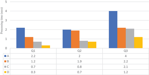
Figure 10. with eight worker nodes.
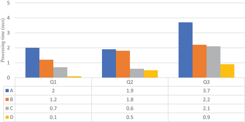
Figure 11. with eight worker nodes.
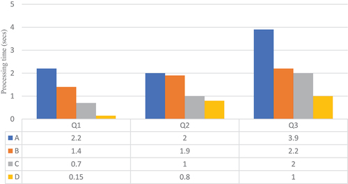
Figure 12. with eight worker nodes.
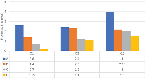
Table 6. Amount of shuffled data for three queries.
4.5. Summary
Based on the presented experimental results, it appears that method D is the most efficient approach. The mediator’s implemented techniques improve the query execution performance of Apache Spark compared to the baseline method A. The findings demonstrate that method B does not offer a significant improvement over the baseline approach. Moreover, method C outperforms method A for all queries, even for low values of . However, our mediator optimization techniques in method D further enhance query optimization by utilizing caching to avoid the precomputation of results that do not change over time and leveraging the broadcast join method to minimize data shuffling. While this method incurs higher memory costs, the storage usage during the benchmark queries was lower than 10 MB per worker machine, which is reasonable. It is worth noting that these optimizations are relevant to the paper’s context, which evaluates continuous queries across integrated streaming and static sources, but they could also be useful in other use cases.
5. Conclusions
In this paper, we have proposed a mediator that integrates big and streaming data in a unified schema on top of Apache Spark. The proposed system addresses the challenges of analyzing streaming geo-reference data without knowledge of big data frameworks. Our system consists of a query parser, a query rewriter, and a query tuner, which manages global and local schemas, and mappings in configuration files and translates the submitted user queries in SQL statements for the Apache Spark application. Our optimization techniques significantly improve the execution performance of the experiment queries compared to Apache Spark native optimizer. Overall, our system provides an efficient and scalable solution for continuous spatial queries over a unified schema. The proposed mediator system can be utilized in various applications such as real-time location-based services, and environmental monitoring. However, the system mainly considers streaming data from messaging queue systems such as Apache Kafka and static data from files such as CSV and JSON. For future work, we aim to support more data sources, both for static data or stream data. Our system optimizes the Apache Spark application plan by pushing down static–static joins and caching partial results. We plan to implement push-down techniques to local sources as it may leverage indexes built in the source databases and reduce the amount of data ingested by Spark engine. Moreover, we also acknowledge that our system requires an integration administrator role to define mappings between local and global schemas. In future work, we aim to study dynamic mapping (Dong et al., Citation2009) in the context of streaming and spatial data to automatically infer mappings at query execution time. Dynamic mapping could eliminate the need for manual mapping definitions and further simplify the mediator system’s integration process.
Supplemental Material
Download MS Word (747.2 KB)Acknowledgements
This research was financed by the French government IDEX-ISITE initiative 16-IDEX-0001 (CAP 20-25) and the PhD is funded by the European Regional Development Fund (FEDER).
Disclosure statement
No potential conflict of interest was reported by the author(s).
Data availability statement
The data that support the findings of this study are openly available in GitHub at https://github.com/AnnaNgo13/streamgeomed.
Supplemental data
Supplemental data for this article can be accessed online at https://doi.org/10.1080/20964471.2023.2275854.
Additional information
Notes on contributors

Thi Thu Trang Ngo
Thi Thu Trang Ngo completed her PhD degree in Computer Science from University Clermont Auvergne, France, in 2023. Prior to that, she received her MS degree in Computer Science from University of Bordeaux, France. Her current research focuses on big spatial data, data integration, and spatial queries within the context of Internet of Things (IoT) environment.

François Pinet
François Pinet holds the position of a research director at the French Research Institute for Agriculture, Food and Environment located in Clermont-Ferrand, France. His research expertise lies in agricultural and environmental information systems. He actively contributes to the field by serving on various scientific committees for conferences and journals related to these domains.

David Sarramia
David Sarramia is an associate professor in Computer Science at University Clermont Auvergne since 2008. His primary areas encompass data management, IoT flow management using NoSQL and indexing technology. Additionally, he actively contributes as a reviewer for the Cluster Computing. Since 2015, he has taken on the role of scientific and technical manager of the CEBA project, a regional data management platform.

Myoung-Ah Kang
Myoung-Ah Kang is currently an associate professor at the University Clermont-Auvergne in Clermont-Ferrand, France. She received her M.Sc. in Computer Science from Pusan National University, Korea in 1996, and later completed her Ph.D. in Computer Science from INSA Lyon, France in 2001. She is a member of the database research group in the laboratory LIMOS (Laboratoire d’Informatique, de Modelisation et Optimisation des Systems, CNRS UMR 6158). Her research primarily focuses on geographical information systems and spatial data warehouse. She also has a keen interest in spatial big data. In addition to her research work, she teaches graduate and undergraduate courses on databases, software engineering and information systems.
Notes
References
- Alam, M. M., Ray, S., & Bhavsar, V. C. (2018, November). A performance study of big spatial data systems. In Proceedings of the 7th ACM SIGSPATIAL International Workshop on Analytics for Big Geospatial Data (pp. 1–9).
- Alam, M. M., Torgo, L., & Bifet, A. (2021). A survey on Spatio-temporal data analytics systems. arXiv E-Prints, arXiv–2103.
- Al Jawarneh, I. M., Bellavista, P., Corradi, A., Foschini, L., & Montanari, R. (2021, October). Efficiently integrating mobility and Environment data for Climate change analytics. In 2021 IEEE 26th International Workshop on Computer Aided Modeling and Design of Communication Links and Networks (CAMAD) (pp. 1–5). IEEE.
- Armbrust, M., Das, T., Torres, J., Yavuz, B., Zhu, S., Xin, R. & Zaharia, M. (2018, May). Structured streaming: A declarative api for real-time applications in apache spark. In Proceedings of the 2018 International Conference on Management of Data (pp. 601–613).
- Armbrust, M., Xin, R. S., Lian, C., Huai, Y., Liu, D., Bradley, J. K. & Zaharia, M. (2015, May). Spark sql: Relational data processing in spark. In Proceedings of the 2015 ACM SIGMOD international conference on management of data (pp. 1383–1394).
- Baig, F., Vo, H., Kurc, T., Saltz, J., & Wang, F. (2017, November). Sparkgis: Resource aware efficient in-memory spatial query processing. In Proceedings of the 25th ACM SIGSPATIAL International Conference on Advances in Geographic Information Systems (pp. 1–10).
- Boucelma, O., Garinet, J. Y., & Lacroix, Z. (2003, November). The virGIS WFS-based spatial mediation system. In Proceedings of the Twelfth International Conference on Information and Knowledge Management (pp. 370–374).
- Carbone, P., Katsifodimos, A., Ewen, S., Markl, V., Haridi, S., & Tzoumas, K. (2015). Apache flink: Stream and batch processing in a single engine. The Bulletin of the Technical Committee on Data Engineering, 38(4).
- Chen, Y., Lu, Y., Fang, K., Wang, Q., & Shu, J. (2020). uTree: A persistent B±tree with low tail latency. Proceedings of the VLDB Endowment, 13(12), 2634–2648. https://doi.org/10.14778/3407790.3407850
- Chintapalli, S., Dagit, D., Evans, B., Farivar, R., Graves, T., Holderbaugh, M. & Poulosky, P. (2016, May). Benchmarking streaming computation engines: Storm, flink and spark streaming. In 2016 IEEE International Parallel and Distributed Processing Symposium Workshops (IPDPSW) (pp. 1789–1792). IEEE.
- Clementini, E., & DiFelice, P. (1996). A model for representing topological relationships between complex geometric features in spatial databases. Information Sciences, 90(1–4), 121–136. https://doi.org/10.1016/0020-0255(95)00289-8
- Dong, X. L., Halevy, A., & Yu, C. (2009). Data integration with uncertainty. The VLDB Journal, 18(2), 469–500. https://doi.org/10.1007/s00778-008-0119-9
- Elastic. 2023. Logstash. Retrieved April , 2023. https://www.elastic.co/logstash/.
- Eldawy, A., & Mokbel, M. F. (2015, April). Spatialhadoop: A mapreduce framework for spatial data. In 2015 IEEE 31st International Conference on Data Engineering (pp. 1352–1363). IEEE.
- Finkel, R. A., & Bentley, J. L. (1974). Quad trees a data structure for retrieval on composite keys. Acta Informatica, 4(1), 1–9. https://doi.org/10.1007/BF00288933
- Gonzalez, J. E., Xin, R. S., Dave, A., Crankshaw, D., Franklin, M. J., & Stoica, I. (2014). {graphx}: Graph processing in a distributed dataflow framework. In 11th USENIX Symposium on Operating Systems Design and Implementation (OSDI 14) (pp. 599–613).
- Grégoire, D. (2015). France Geojson. https://github.com/gregoiredavid/france-geojson.
- Guttman, A. (1984, June). R-trees: A dynamic index structure for spatial searching. In Proceedings of the 1984 ACM SIGMOD International Conference on Management of Data (pp. 47–57).
- Halevy, A. Y. (2001). Answering queries using views: A survey. The VLDB Journal, 10(4), 270–294. https://doi.org/10.1007/s007780100054
- Inoubli, W., Aridhi, S., Mezni, H., Maddouri, M., & Nguifo, E. M. (2018, August). A comparative study on streaming frameworks for big data. In VLDB 2018-44th International Conference on Very Large Data Bases: Workshop LADaS-Latin American Data Science (pp. 1–8).
- Karimov, J., Rabl, T., Katsifodimos, A., Samarev, R., Heiskanen, H., & Markl, V. (2018, April). Benchmarking distributed stream data processing systems. In 2018 IEEE 34th international conference on data engineering (ICDE) (pp. 1507–1518). IEEE.
- Kreps, J., Narkhede, N., & Rao, J. (2011, June). Kafka: A distributed messaging system for log processing. Proceedings of the NetDb, 11(2011), 1–7.
- Kwon, Y., Balazinska, M., & Greenberg, A. (2008). Fault-tolerant stream processing using a distributed, replicated file system. Proceedings of the VLDB Endowment, 1(1), 574–585. https://doi.org/10.14778/1453856.1453920
- Lee, J. G., & Kang, M. (2015). Geospatial big data: Challenges and opportunities. Big Data Research, 2(2), 74–81. https://doi.org/10.1016/j.bdr.2015.01.003
- Lenzerini, M. (2002, June). Data integration: A theoretical perspective. In Proceedings of the twenty-first ACM SIGMOD-SIGACT-SIGART Symposium on Principles of Database Systems (pp. 233–246).
- Mahmood, A. R., Aly, A. M., Qadah, T., Rezig, E. K., Daghistani, A., Madkour, A., Abdelhamid, A. S., Hassan, M. S., Aref, W. G., & Basalamah, S. (2015). Tornado: A distributed spatio-textual stream processing system. Proceedings of the VLDB Endowment, 8(12), 2020–2023. https://doi.org/10.14778/2824032.2824126
- Meng, X., Bradley, J., Yavuz, B., Sparks, E., Venkataraman, S., Liu, D. & Talwalkar, A. (2016). Mllib: Machine learning in apache spark. The Journal of Machine Learning Research, 17(1), 1235–1241.
- OGC. 2023. Open Geospatial Consortium. Retrieved April , 2023. https://www.ogc.org/.
- Pandey, V., Kipf, A., Neumann, T., & Kemper, A. (2018). How good are modern spatial analytics systems? Proceedings of the VLDB Endowment, 11(11), 1661–1673. https://doi.org/10.14778/3236187.3236213
- Robert, H. (2003). Spatial data analysis theory and practice. Journal of Women S Health.
- Sedona, Apache. 2022. Apache Sedona. Retrieved November , 2022. https://sedona.apache.org/.
- Shaikh, S. A., Mariam, K., Kitagawa, H., & Kim, K. S. (2020, October). GeoFlink: A distributed and scalable framework for the real-time processing of spatial streams. In Proceedings of the 29th ACM International Conference on Information & Knowledge Management (pp. 3149–3156).
- Shvachko, K., Kuang, H., Radia, S., & Chansler, R. (2010, May). The hadoop distributed file system. In 2010 IEEE 26th Symposium on Mass Storage Systems and Technologies (MSST) (pp. 1–10). IEEE.
- Storm, Apache. 2014. ApacheStorm. Retrieved October , 2022. https://storm.apache.org/.
- Stripelis, D., Anastasiou, C., & Ambite, J. L. (2018, June). Extending apache spark with a mediation layer. In Proceedings of the International Workshop on Semantic Big Data (pp. 1–6).
- Tang, M., Yu, Y., Mahmood, A. R., Malluhi, Q. M., Ouzzani, M., & Aref, W. G. (2020). Locationspark: In-memory distributed spatial query processing and optimization. Frontiers in Big Data, 3, 30. https://doi.org/10.3389/fdata.2020.00030
- Tantalaki, N., Souravlas, S., & Roumeliotis, M. (2020). A review on big data real-time stream processing and its scheduling techniques. International Journal of Parallel, Emergent and Distributed Systems, 35(5), 571–601. https://doi.org/10.1080/17445760.2019.1585848
- Tatbul, N. (2010, March). Streaming data integration: Challenges and opportunities. In 2010 IEEE 26th International Conference on Data Engineering Workshops (ICDEW 2010) (pp. 155–158). IEEE.
- Toshniwal, A., Taneja, S., Shukla, A., Ramasamy, K., Patel, J. M., Kulkarni, S. & Ryaboy, D. (2014, June). Storm@ twitter. In Proceedings of the 2014 ACM SIGMOD International Conference on Management of Data (pp. 147–156).
- Vavilapalli, V. K., Murthy, A. C., Douglas, C., Agarwal, S., Konar, M., Evans, R. & Baldeschwieler, E. (2013, October). Apache hadoop yarn: Yet another resource negotiator. In Proceedings of the 4th annual Symposium on Cloud Computing (pp. 1–16).
- Wiederhold, G. (1992). Mediators in the architecture of future information systems. Computer, 25(3), 38–49. https://doi.org/10.1109/2.121508
- Wood, J. (2008). Filter and Refine Strategy. In Encyclopedia of GIS. Springer US.
- Xie, D., Li, F., Yao, B., Li, G., Zhou, L., & Guo, M. (2016, June). Simba: Efficient in-memory spatial analytics. In Proceedings of the 2016 International Conference on Management of Data (pp. 1071–1085).
- You, S., Zhang, J., & Gruenwald, L. (2015, April). Large-scale spatial join query processing in cloud. In 2015 31st IEEE International Conference on Data Engineering Workshops (pp. 34–41). IEEE.
- Yu, J., Wu, J., & Sarwat, M. (2015, November). Geospark: A cluster computing framework for processing large-scale spatial data. In Proceedings of the 23rd SIGSPATIAL International Conference on Advances in Geographic Information Systems (pp. 1–4).
- Zaharia, M., Chowdhury, M., Das, T., Dave, A., Ma, J., McCauly, M. & Stoica, I. (2012). Resilient distributed datasets: A {Fault-Tolerant} abstraction for {In-memory} cluster computing. In 9th USENIX Symposium on Networked Systems Design and Implementation (NSDI 12) (pp. 15–28).