An alignment- and reference-free strategy using k-mer present pattern for population genomic analyses

ABSTRACT

Pangenomes are replacing single reference genomes to capture all variants within a species or clade, but their analysis predominantly leverages graph-based methods that require multiple high-quality genomes and computationally intensive multiple-genome alignments. K-mer decomposition is an alternative to graph-based pangenomes. However, how to directly use k-mers for the population genetic analyses is unknown. Here, we developed a novel strategy that uses the variants of k-mer count in the genome for population analyses. To test the effectivity of this method, we compared it directly to the SNP-based method on the analysis of population structure and genetic diversity of 267 Saccharomyces cerevisiae strains within two simulated datasets and a real sequence dataset. The population structure identified with k-mers recapitulates that obtained using SNPs, indicating the effectiveness of k-mer-based approach, and higher genetic diversity within real dataset supported k-mers contained more genetic variants. Based on k-mer frequency, we found not only SNP but also some insertion/deletion and horizontal gene transfer (HGT) fragments related to the adaptive evolution of S. cerevisiae. Our study creates a framework for the alignment- and reference-free (ARF) method in population genetic analyses, which will be more pronounced in the species with no complete genome or highly diverged species.

KEYWORDS:

• K-mers
• population genomics
• genetic diversity
• alignment-free
• reference-free

1. Introduction

Molecular population genomics is the study of quantifying the level of genetic variations within and among populations and identifying the evolutionary driving forces that shape these variations at a genomic level (Casillas and Barbadilla 2017; Johnston et al. 2019). With the development of sequencing techniques, the analysed sequences have been extended from a single gene to a whole genome, and the type of variation also extends from a single-point mutation to large-scale structural variants. Numerous studies have demonstrated capturing more genetic variants among a species generally provided a more accurate population genetic analysis. However, the most common method for the identification of genetic variants is by aligning short reads to a reference genome, which results in reference bias (Parfrey et al. 2008; Ballouz et al. 2019). To capture the entire genomic variations of a species, pangenomes have emerged in recent years (Qin et al. 2021; Bayer et al. 2022; Li et al. 2022). Using a pangenome as a reference offers the opportunity to study the entire genomic diversity of a population, including structurally complex regions (Zhou et al. 2022; Wang et al. 2023). Currently, the most advanced method for pangenome construction and analysis is the graph-based strategy (Chen et al. 2019; Rakocevic et al. 2019; Sirén et al. 2021). However, this strategy is still in the early development stage and lacks a standard approach for graph-based pangenome construction and analysis. Furthermore, the accuracy of this method relies on the quality of selected genomes for pangenome construction, but a high-quality genome is difficult to obtain for most species.

As alternatives to reference-based methods, several alignment-free approaches have been developed for variant calling independent reference. For example, Cortex identified variants with the coloured de Bruijn graphs (Iqbal et al. 2012). kSNP v2 uses the matched length of k-mer to find SNPs (Gardner and Hall 2013). PanGenie and KAGE are based on reference- and allele-specific k-mers or k-mer count to validate SNP, insertion and deletion mutation (Ebler et al. 2022; Grytten et al. 2022). Furthermore, present/absent variants (PAVs) of k-mer can directly associate with phenotypes (Lees et al. 2016; Rahman et al. 2018; Voichek and Weigel 2020). k-mer-based genome-wide association study (GWAS) not only recapitulates those found with SNPs but also finds structural variants and regions missing from reference genomes responsible for phenotypic variation (Rahman et al. 2018; Voichek and Weigel 2020). In addition, some tools have been developed for the downstream analyses in population, like PanKmer which uses the present-absent value of k-mers for sequence similarity statistics and identifying cases of hybridisation (Aylward et al. 2023), PanTools based on k-mer count to find strain- and phenotype-specific barcodes and estimate the similarity between genomes (Jonkheer et al. 2022). These applications inspired us to develop a method that directly uses k-mers to perform population genetic analyses.

In population genetic analyses, phylogenetic tree construction, principal component analysis (PCA), and genetic structure analysis are the common three approaches to investigate the genetic differentiation among populations, and a series of summary statistical methods (like S, π, SFS) is helpful for elucidate the association between genetic variations with genetic diversity and other related biological problems. K-mer-based method in phylogenetic tree construction has a long history (Reinert et al. 2009; Yi and Jin 2013; Haubold 2014; Zielezinski et al. 2017; Ren et al. 2018). The k-mer-based phylogenetic trees of the viruses, prokaryotes (Qi et al. 2004; Bromberg et al. 2016) and eukaryotic species [fungi (Wang et al. 2009), plants (Hatje and Kollmar 2012), and mammals (Sims et al. 2009)] were extremely similar to the species trees created by the manually curated NCBI taxonomic database. However, few studies focused on the application of k-mers in other population genetic analyses.

In this study, we developed a strategy that directly used the k-mer copy number in the genome to explore the population structure and assess the genetic diversity of species. A published dataset that contained 266 Saccharomyces cerevisiae genomes was selected as a test (Duan et al. 2018). The main reason was these isolates possessed a high level of genetic diversity (about one SNP per 13 bases), a complex population structure (about 20 subpopulations), and a lot of structural variations (SVs) and lineage-specific large alien fragments obtained through horizontal gene transfer (HGT) and introgression from other species within the genus Saccharomyces (Duan et al. 2018). When we only used a single reference (such as S288C), most information about SVs and alien fragments would be ignorance. Thus, the dataset was suitable for us to explore the importance of the reference-free method. To test the effectiveness of this strategy, we generated two simulated datasets that only contained SNP sites, and compared them directly to the conventional SNP-based approach. Furthermore, we re-analysed the population structure of these 266 isolates with de nova assembled genome sequences, and found k-mer-based method had a higher resolution to differentiate the population structure and capture not only SNPs but also indels and HGT fragments that were related to yeast domestication.

2. Materials and methods

2.1. S. cerevisiae genome collection

Our study comprised 267 S. cerevisiae accessions. One of them was the S288c genome (version R64-1-1), which was widely used as the reference genome in population analyses of S. cerevisiae. The remaining genome sequences were downloaded from the National Center for Biotechnology Information (NCBI) with the Bioproject ID, PRJNA396809.

2.2. The description of used datasets

To test the effectiveness of the k-mer-based method in population genetic analyses, we first generated two simulated sequence databases that only contained SNP sites. The SNP sites were obtained by mapping the de novo assembled contigs to the S288c genome using the LastZ programme with default settings, and the custom Python scripts were applied to extract the variants. A total of 885,291 high-quality reference-based SNPs were detected across the 266 genomes. Then, we randomly selected 81,152 SNP sites with the interval between adjacent SNPs above 100 bp to generate 266 simulated sequences (database 1). The simulated sequences in database 2 were generated 266 simulated sequences using all of the SNP sites. The final database (database 3) contained the de novo assembled contigs for 266 S. cerevisiae strains. The reads-calling SNPs were obtained through mapping reads to the S288c genome. The variation sites of an isolate with a coverage depth lower than 15 and greater than four times of the sequence depth of the isolate were excluded. Detailed information about SNP calling was provided by Duan et al. (2018). The pipeline for k-mer-based population genetic analyses was shown in Figure S1.

2.3. k-mer table generation

Lack of alignment made it more difficult to keep the identical k-mer derived from homology regions of the genome. Fortunately, for sufficiently large k, any given k-mer was approximately unique to a sequence, so in the absence of extenuating circumstances (e.g. strong mutational bias or low-complexity regions), the shared k-mer was likely to be homology among samples (homology) (Fan et al. 2015; Bernard et al. 2019). The threshold k was determined by genome size and sequence complexity (Fan et al. 2015). However, longer k-mer increased the possibility that a k-mer covered multiple mutations. If a k-mer covered multiple variants, it counted equally as one carrying only a single mutation event, and its count pattern was consistent with the combination of variants (Figure S2). Consequently, the more sequence variations that were present the smaller k must be to avoid a k-mer carrier multiple variants. Due to the density of genetic variants being unknown, an optimal k value was the minimum length that kept k-mer homology in the genome.

To select the minimum length to maintain k-mer homology, the percentage of unique k-mers among total k-mers from 23 strains was calculated at k = 13–31, respectively. The selected strains covered all identified lineages and sources of the 266 strains (Duan et al. 2018), thus it was reasonable to use them to denote the complexity of S. cerevisiae genomes. When the fraction of unique k-mers reached a plateau, the k value was the minimum length to keep k-mer homology (Gardner and Hall 2013). The extraction and counting of k-mers in a genome used a sliding window approach to eliminate the influence of an arbitrarily chosen starting point. The adjacent k-mers overlapped for k-1 nucleotides in the output file.

Having identified the optimal length, we extracted the k-mers from all genomes and merged them into an m × n matrix. m was the number of samples, and n was the total k-mers that were present in all analysed genomes. In the k-mer matrices, the number denoted k-mer count in a genome.

2.4. Phylogenetic analysis and principal components analysis

The phylogenetic distance D between two samples was estimated using the metric (Fan et al. 2015):

$\mathit{D}=-\frac{1}{k}\mathit{ln}\frac{{\mathit{n}}_{\mathit{sk}}}{n_{\mathit{tk}}}$

where $n_{\mathit{sk}}$ was the number of k-mers that were shared between samples, and $n_{\mathit{tk}}$ was the total number of k-mers in the two samples (Fan et al. 2015). For SNPs, the phylogenetic distance D between two samples was:

$\mathit{D}=-\mathit{ln}\frac{n_s}{n_t}$

where $n_s$ was the number of SNPs shared between samples, and $n_t$ was the genome size.

The distances were computed pairwise and assembled into a triangular matrix, and then we put this matrix into MEGA X to generate the NJ trees (Kumar et al. 2018). The NJ trees were visualised using FigTree v1.4.3. Comparison between SNP- and k-mer-based NJ trees was assessed using the Robinson-Foulds distance calculated with the treedist programme of the Phylip package (Robinson and Foulds 1981; Felsenstein 1989).

Principal component analysis (PCA) that was based on k-mer count and SNPs matrix were conducted using the Python 3.7.3 package sklearn.decomposition (Pedregosa et al. 2011). Pearson correlation analyses were performed between SNP and k-mer-based principal components (PC) to explore the power of k-mer count in the discrimination of the sample.

2.5. Population structure analyses

We used ADMIXTURE v1.3.0 to assess the population genetic structure (Alexander et al. 2009). Before this analysis, the k-mers present in a genome were selected as reference, since the neo k-mers in other samples were carriers of the allele-specific k-mers (Ebler et al. 2022). Considering the importance of position information in linkage disequilibrium (LD) analyses, only the unique k-mers were used for further study. The unique k-mers and SNP matrixes were transformed into .ped and .maf files using our python3 script and then transformed into the binary format file using PLINK v1.07 (Purcell et al. 2007). PLINK V1.07 implemented LD pruning with the function indep-pairwise (50 5 0.2) and MAF > 0.01. This function calculated pairwise r² in a 50-variants-window, shifts at a pace of five variants, and excluded one pair of variants when r² > 0.2. After pruning out, ADMIXTURE v1.3.0 was performed to assess population genetic structure, and the best-fit K value was determined by the cross-validation (CV) procedure of the programme and the value with a minimum CV error was optimal (Alexander and Lange 2011).

2.6. Genetic diversity analyses

Nucleotide diversity (θπ) was calculated as the average number of variable sites in each pairwise sequence comparison. It was mathematically defined by:

${\theta }_{\pi }=\frac{1}{C_n^2}{\sum }_{i=1}^{n-1}{\sum }_{j=i+1}^n\frac{\mathit{Sij}}{L}$

where $S_{\mathit{ij}}$ was the number of different nucleotides between sequence i and sequence j, $C_n^2$ represented the number of pairwise comparisons, and L was the sequence length. However, the change of k-mer count not only mutations caused by nucleotide substitutions but also insertions and deletions (indels), which made each pairwise sequence comparison had a different total k-mer number ($n_t$). To account for this, we used the length of the sequences in each pairwise comparison instead of a fixed L.

${\theta }_{\pi }=\frac{1}{k}\frac{1}{C_n^2}{\sum }_{i=1}^{n-1}{\sum }_{j=i+1}^n\frac{1}{2}(\frac{{\mathit{S}}_{\mathit{kij}}}{n_{\mathit{ti}}}+\frac{{\mathit{S}}_{\mathit{kji}}}{n_{\mathit{tj}}})$

$S_k$ was the number of different k-mers between sequence i and j. $S_{\mathit{kij}}$ was the number of k-mers present in sequence i, and $S_{\mathit{kji}}$ was the number of k-mers present in sequence j. $n_{\mathit{ti}}$ was the total k-mers that present in sequence i, while $n_{\mathit{tj}}$ was the total number of k-mers present in sequence j. The coefficient $1/\mathit{k}$ was added due to a base being covered by k k-mers.

2.7. Detecting potential indels or HGT fragments

Unlike SNPs, indels introduced the complication of changing k-mers. For example, a single insertion of length l caused the loss of at most (k − 1) k-mers and a gain of at most (l + k − 1) k-mers, while a single deletion of length l caused the loss of at most (l + k − 1) k-mers and a gain of at most (k − 1) k-mers. Therefore, the number of affected k-mers was extrapolated using the size of the indels (Lee et al. 2020). However, different from previous studies that only focused on the changing k-mer number between a pair of samples, the identification of indel in our method was based on the r² between adjacent k-mers. If over k continues k-mers possessed consistent present pattern (r² = 1), these k-mers might be derived from the same potential indel (Figure S3). Dense genetic variants were a noise in this analysis. For example, two closer SNP sites with r² = 1 could also generate more than k continues k-mers (Figure S4a). The indels might also be missed when another mutation happened in the indel site (Figure S4b).

2.8. Adaptive evolution analyses

To widen the genetic variants detected in yeast domestication, such as major rearrangements, insertions, and deletions, the k-mer-based joint allele frequency spectrum across wild and domesticated groups, LSF and SSF-groups, were calculated, respectively. The k-mers that were shared by above 90% of isolates in one group but absent in no more than 10% of isolates strains in another group were identified as group-specific k-mers. The domesticated group-specific k-mers were defined as favourable k-mers, while the wild group-specific k-mers were defined as unfavourable k-mers. The six isolates from lineage CHN-VIII belonged to the domesticated population and LSF group. For LSF and SSF groups, the group-specific k-mers present in less than half of wild isolates were recognised as a candidate for the divergence of liquid- and solid-fermentation states. Blastn was used to align group-specific k-mers to the genome or genes annotated of the corresponding isolate. GO and Kyoto Encyclopaedia of Genes and Genomes enrichment analysis were performed for the favourable gene sets using DAVID (https://david.ncifcrf.gov/home.jsp) with a cut-off of FDR < 0.05.

3. Results

3.1. Overview of k-mer tagged variations in population

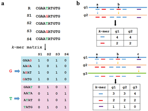
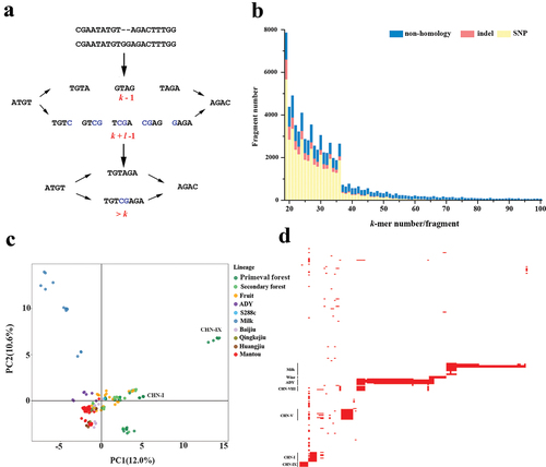
In our method, we used the k-mer count as an allelic contrast instead of defining genetic variants in a population relative to a reference genome. The main question was how to keep the consistency between the pattern of k-mer count and its coverage variation in a population. If the variants generated novel k-mers (neo k-mers), this question was easily resolved. For instance, a substitution, such as a T to G, made four k-mers that carrier T transformed into four neo k-mers (length of four bases) that carrier G, and the pattern of k-mer were consistent which its covered allele at the population level (Figure 1a). However, when k-mers possessed multiple copies in the genome (k-mer homoplasy), the situation would be complex (Figure 1b). For example, if a mutation makes k-mer1 () in g1 turn into another k-mer2 () that already exists elsewhere in the genomes of g2, meanwhile another mutation makes k-mer2 turn into k-mer1, so these mutations would be ignored (Figure 1b). With the increase of analysed genomes, the change of k-mer with multiple copy numbers would be more complex (Figure 1b). Thus, one of the most important properties of a k-mer was the uniqueness of its sequence.

Figure 1. k-mer count and genetic variations. (a) The unique k-mer and its tagged SNP site, illustrated here for overlapping k-mers (k = 4, stride = 1) in four sequences. (b) The k-mers with multiple copies and their tagged SNPs. The box with colour denoted the type of k-mer. a, b and c denoted the SNP sites.

3.2. Choosing an optimal k-mer length

k-mer length was a critical parameter in determining the uniqueness of k-mer in the genome. To select an optimal k-mer length, we first calculated the ratio of unique k-mer in the genomes of 23 strains at different k values. The increased curves of unique k-mers in these strains were consistent, which were increased sharply at k = 13–15, and reached a plateau at k = 18. At k = 18, about 98% k-mers were unique in the yeast genome, and longer lengths led to only minimal increases (<0.4% with 31 bp) (Figure S5). The sequence of k-mers with multiple copies generally was simple, such as oligo (A)₁₈. These k-mers cannot be unique within a genome because of duplication and the possible presence of multiple copies of mobile elements within the genome. Thus, we choose the k-mer with 18 bases for further study.

3.3. Filtering out the k-mer with multiple copies

Using k-mer count as allelic contrast, we found above 99% of polymorphic k-mers possessed two alleles in simulated datasets (Figure S6). For the biallelic k-mers, the k-mers with 0 and 1 copy accounted for about 98% of the total. For the k-mers with three alleles, the alleles were generally 0, 1, and 2, and one of them was low frequency (<0.01). To avoid the effects of k-mers with multiple copies, we remained k-mers that possessed less than five alleles which account for 99.9% of the total, and the k-mers with more than 2 copies in the genome account for less than 0.01%. The sequences of filtered out k-mers were generally simple, such as oligo (N) and short tandem repeats. Mapping these k-mers to the genome found that these k-mers mainly derived from the repetitive regions or heterochromatin, such as telomeres or GC-enriched regions (Figure S7). After filtering out, the remaining number of k-mers was nearly equal in all samples, and accounted for above 98% of total k-mers in each sample (Table S1).

In dataset 1, all SNP sites were tagged by k-mers and only 0.26% of SNP sites were not tagged by k k-mers (Figure S8a). In dataset 2, 0.5% SNP sites were not tagged by k-mers, and 3% k-mer was not tagged by k k-mers (Figure S8a). Mapping reads to S288c identified 75,990 (about 93.6%) in dataset 1 and 810,169 (about 91.5%) SNP sites in dataset 2, but nearly all real-calling SNP sites were tagged by k-mers (Figure S8b). The main reason might be the missing SNP sites in the k-mer-based method mainly located in repetitive regions of genomes, and in a reads-calling method not only derived from the repetitive regions (with higher coverage depth), but also the regions with low coverage depth. In real datasets, the number of remaining k-mers was 30,257,427, which was higher than that obtained in dataset 2. Among them, the k-mers that covered SNP sites accounted for about 70% of the total. In each strain, about 2% of k-mers that derived from no-homology with S288C, while 2.5% of k-mers derived from non-SNP mutations (Table S2).

3.4. k-mer- and SNP-based methods obtained consistent patterns of population structure

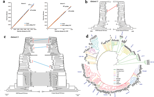
Quantitative comparison between k-mer and SNP based-trees showed high similarity concerning branch lengths; there was a high correlation between their patristic distances (r² = 1 and 0.9996 for dataset 1 and dataset 2, respectively) (Figure 2a) and a low Branch Score Distance (BSD = 0.000011 and 0.00205 for dataset 1 and dataset 2, respectively). Compared to the NJ-trees based on SNP, the Symmetric Difference was 6 and 56 for k-mers-based and reads-calling SNP-based NJ-trees for dataset 1, while 44 and 52 for k-mer-based for dataset 2. The difference among NJ-trees was focused on a few clades with shorter branch lengths, such as the clade [(HLJ3:HLJ2):JL4] and [(BJ28:SD3):FJ12):XJ6):BJ7] in dataset 1, but the relationship between lineages were consistent (Figure 2b,c). Detailed information about NJ-trees were shown in Figure S9–S14. Using the k-mers extracted from real sequences (dataset 3), the obtained lineages in the phylogenetic tree recapitulated the results obtained using SNPs (Figure 2d), but the pairwise distances were greater than that calculated using the k-mers in dataset 2 (Figure S15), indicating there were non-SNPs variants between the real sequences. The wild isolates were clustered into nine clear lineages and CHN-IX represents the most basal lineage of S. cerevisiae. The domesticated strains fall into two major monophyletic groups associated with solid- and liquid-state fermentation (Figure 2d). In the SSF group, strains associated with Baijiu, Huangjiu, and Qingkejiu fermentation formed three distinct lineages, while the strains associated with Mantou fermentation were clustered mainly into seven lineages. In the LSF group, the strains associated with molasses fermentation formed the lineage milk, but the clade wine was clustered together with the lineage ADY.

Figure 2. The comparisons between k-mer- and SNP-based NJ-trees. (a) The association between k-mer- and SNP-based pairwise distance in dataset 1 and dataset 2, respectively. (b) The comparisons between the topology of the NJ-trees that were constructed using k-mers and SNPs from dataset 1. The red line indicated the difference between the NJ-trees. (c) The comparisons between the topology of the NJ-trees that were constructed using k-mers and SNPs from dataset 2. The difference mainly focused on the lineage CHN-V that marked by a grey box. (d) The NJ-tree that constructed using the polymorphic k-mers from dataset 3.

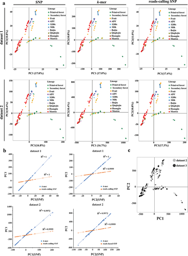
In PCA results, the clustered pattern obtained using k-mer and reads-calling SNP was consistent with that obtained using SNPs in datasets 1 and 2 (Figure 3a). Association analyses showed the values of PC1 and PC2 obtained using PAVs of k-mer and read-mapping SNPs were strongly associated (r² > 0.99) with that corresponding to those obtained using SNPs (Figure 3b), and the contribution of PC1, PC2, PC3, and PC4 that obtained using k-mers were closer to SNPs than read-calling SNPs (Table S3). In real dataset 3, the cluster relationship was consistent with that obtained in NJ-trees, but k-mers contained more variants among sequences, thus the PCA results from k-mers provided a higher resolution to differentiate the population structure than that obtained from SNP (Figure 3c).

Figure 3. The comparison of k-mers and SNP-based principal component analyses (PCA). (a) PCA were based on different genetic markers from dataset 1 and dataset 2, respectively. (b) Correlation between SNP- and k-mers based PC1 and PC2 in dataset 1 and dataset 2, respectively. (c) The comparison of PCA results that based on k-mer counts from dataset 2 (grep) and dataset 3 (black).

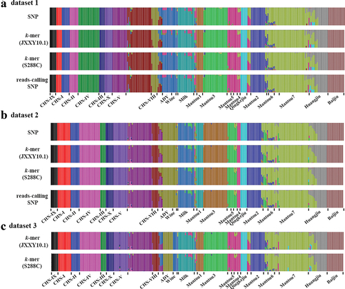
In the k-mer matrix, several k-mers carrier the same variant, and the k-mers denote all the allelic states of these variants. Thus, before analyses, we choose the k-mers that were present in the genome as a reference. These k-mers only carried the reference-based allelic states, and then implemented linkage disequilibrium (LD) pruning using PLINK. Considering the importance of position information in the LD pruning, we only use the unique k-mers because their relative positions in a genome were easily obtained based on their extracted order. To explore the effect of reference selection, we selected the k-mers in strain S288C and JXXY10.1 as a reference, respectively. In dataset 1, the r² between pairwise k-mers in the window of k was 1. After LD pruning with (r² = 1), the remaining k-mers were 78,767 and 78,568 when using JXXY10.1 and S288C as reference, respectively. These values were slightly less than the number of SNPs (81,152) but more than the number of reads-calling SNPs (75,990). In dataset 2, we excluded a pair of SNPs and k-mers when r² > 0.2 in 50-variants in a window and finally obtained 131,331 SNP, 130,080 reads-calling SNPs, 150,794 JXXY10.1-based k-mers and 150,997 S288c-based k-mers. The optimal k value and population structure using k-mers or reads-calling SNPs were consistent with that obtained using corresponding SNPs (Figure 4a,b, and S16). For real dataset 3, the lineage ADY and wine were divided into two genetic populations, indicating the divergence between lineages wine and ADY was increased when the genome included more genetic variants. The consistent results that obtained using JXXY10.1-based and S288c-based k-mers indicated that reference selection did not affect k-mer-based population genetic structure analyses (Figure 4c).

Figure 4. The genetic clustering patterns of Saccharomyces cerevisiae using different variants at K = 20 in dataset 1 (a) in dataset 2 (b) and dataset 3 (c). Isolates in each identified population are consistent with that identified in the phylogenetic tree presented in Figure 2.

3.5. k-mer-based methods obtained higher genetic diversity than SNP-based methods in real dataset

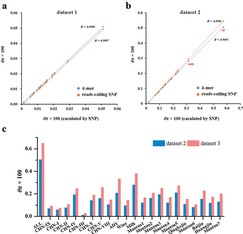
In dataset 1, nearly all alleles were tagged by k-mers, thus the k-mer-based θπ within the group was equal to that calculated using SNPs, and its power in assessment θπ was higher than that calculated using reads-based SNPs (Figure 5a). In dataset 2, a small proportion of SNP sites between pairwise samples closer together (closer than k), resulting in a k-mer carrier multiple substitutions was counted equally as one carrying only a single substitution. Fortunately, most of these SNPs are present at very low frequencies, with 25.7% of the polymorphic positions being singletons and 80% with a minor allele frequency (MAF) < 0.05 (Figure S17), implying the k-mers that carrier multiple variants only present in a rare individual. Thus, the k-mer-based θπ were slightly lower but strongly associated (r² > 0.9995) with that calculated by simulated SNPs (Figure 5b). The genetic diversity based on the reads-mapping SNPs within most lineage was nearly equal to the k-mer-based method (Figure 5b). In real dataset 3, the k-mers expand the type of genetic variants, thus the genetic diversity based on k-mers count was higher than that calculated using the k-mers derived from SNPs (Figure 5c).

Figure 5. k-mer- and SNP-based nucleotide diversity (θ_π) within different groups of Saccharomyces cerevisiae. (a) and (b) the association between the genetic diversity that calculated by SNP and k-mers or reads-mapping-based SNPs in dataset 1 and dataset 2, respectively. (c) The genetic diversity within different groups that calculated by k-mers from dataset 2 and dataset 3.

3.6. k-mer-based methods can detect potential large-scale variants in the real dataset

Insertions/deletions fragments generally affect more than k continues k-mers (Figure 6a). If these k-mers are derived from the same mutation event, they theoretically possess the same present pattern in a population (r² = 1). Based on this principle, we calculated the r² between adjacent k-mers, and obtained 64,774 fragments with more than k continues k-mers across 267 S. cerevisiae genomes. Most were small-scale variations with low frequency (Figures S18 and S19). However, most small-scale variations (≤18 bp, 36 k-mers) were derived from complete linkage SNPs instead of deletion/insertion. With the increase in fragment size, the probability of fragments derived from SNP was decreased (Figure 6b). Nearly all large fragments (≥60 k-mers) were derived from the non-homology region with S288c. PCA analyses using PAVs of fragments containing more than 60 k-mers insertion/deletion showed the strains from primaeval forest and yak milk were separated from the others (Figure 6c), indicating these strains contained more non-SNP variations. Further analyses found the large fragments with more than 500 k-mers were lineage-specified and mainly derived from CHN-IX, CHN-I, and CHN-V and liquid-state fermentation lineages (ADY, Milk, and Wine) (Figure 6d). Mapping them to the corresponding genome, we found that they were mainly located in 15 previously identified HGT or introgression fragments (Table S4) (Duan et al. 2018). In the lineage Milk, these lineage-specific HGT fragments contained several genes involved in galactose utilisation, including GAL2 encoding galactose transporter, GAL7-GAL10-GAL1 cluster of the galactose metabolism network, phosphoglucomutase 1 (PGM1), and phosphomutase (PMU1) cluster. PGM1 and PMU1 were the new finding in the k-mer-based method.

Figure 6. k-mers and insertions/deletions. (a) The principle for k-mers was to identify insertion. (b) The source of the fragments assembled with more than k k-mer in dataset 3. (c) The principal component analysis used the PAVs of fragments with more than k k-mers. (d) The possible horizontal gene transfer (HGT) fragments (≥500 k-mer) in each strain. The order of strains is based on the phylogenetic tree presented in Figure 2d.

3.7. k-mer-based method allowed the detection of a wider range of genetic variants responsible for yeast domestication

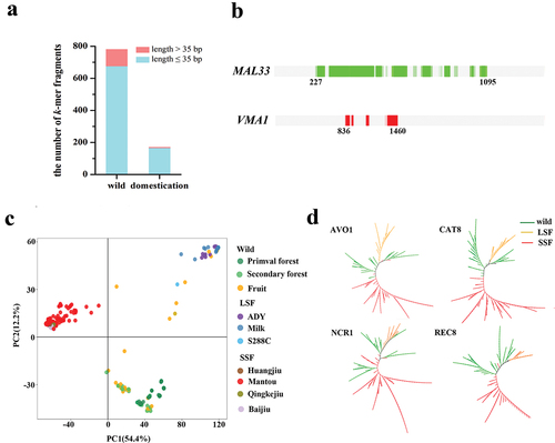
Comparative analyses of k-mer frequency between wild and domesticated groups identified 171 k-mer fragments (variations) with higher frequency in domesticated groups (Figure 7a). The longest fragments (125 k-mers) were present in the nuclear gene VMA1, whereas a longer fragment of the maltase transcription activator gene MAL33 was deleted from the domesticated group (Figure 7b). Previous studies that based on pan-genome datasets also found VDE is an adaptation for horizontal transfer fragments (Han et al. 2021). Further analyses found that the fixed fragments in domesticated isolates were derived from 89 genes (Table S5). Gene Ontology (GO) enrichment analysis showed that the 89 genes were enriched in seven terms, including mitotic nuclear division, cell cycle, regulation of GTPase activity, proton transport, folic acid-containing compound metabolic process, glutamyl-tRNA aminoacylation, and mitotic nuclear division (Table S6). Comparative analyses of k-mer frequency between LSF- and SSF-groups identified 1,034 and 1,431 LSF- and SSF-group-specific variants, respectively (Figure S20 and S21). PCA using these group-specific k-mers obtained three groups (wild, LSF, and SSF) (Figure 7c). If the k-mers present in more than 50% of wild isolates denote ancestor alleles, we identified 191 and 248 candidate genes that were associated with LSF and SSF, respectively (Table S7 and S8). The genes AVO1, CAT8, NCR1, and REC8 harboured the highest number (10–17) of group-specific mutations. The phylogenetic tree using k-mer of a single gene showed that the LSF and SSF strains were divergent (Figure 7d). Enrichment analyses showed cell cycle and DNA repair suffered more selective pressure in the SSF group, while inter-strand cross-link repair was the most enriched in LSF groups (Table S9).

Figure 7. Fix and lose k-mers during domestication. (a) The number of fixed k-mer fragments in wild and domesticated populations. (b) The distribution of fixed k-mers in MAL33 of wild isolates (green) and VMA1 in domesticated isolates (red). (c) Principal component analysis using the PAVs of group-specific k-mers. (d) Unrooted phylogenetic trees of 267 Saccharomyces cerevisiae isolates constructed from PAVs of k-mers extracted from genes AVO1, CAT8, NCR1, and REC8, respectively.

4. Discussion

Since the early days of the genome era, the scientific community has relied on a single “reference” genome for each species, which is used as the basis for a wide range of genetic analyses, including studies of variation within and across species. As sequencing costs have dropped, thousands of new genomes have been sequenced, and scientists have come to realise that a single reference genome is inadequate for many purposes. To capture the entire genomic diversity of a population, some studies have been used pangenome as a reference (Zhou et al. 2022; Wang et al. 2023), while others had been developed alignment-free methods that use k-mers instead of defining genetic variants in a population relative to a reference genome in GWAS (Jaillard et al. 2018; Rahman et al. 2018; Voichek and Weigel 2020). Compared to the pan-genome, the methods based on k-mers were easier and cheaper since the k-mers can be directly extracted from raw short reads or the genome assembled by them. In the present study, the k-mers were directly extracted from the assembled genome, which avoids the effect of sequence depth. Furthermore, we use the k-mer count in the genome as variants, which have more power than to describe the number of mutations. Practically, k-mer count can incorporate the copy number variations. Rahman et al. (2018) found tests based on k-mer counts are likely to have more power, making the detection of association with a smaller number of samples possible (Rahman et al. 2018). To avoid k-mer homoplasy, we choose a enough large k that make nearly all k-mers unique, and then filtered out the k-mers that occurred multiple mutations (possessed multiple alleles in the population). The sequences of k-mers with multiple copies were generally simple and mainly derived from repetitive regions or heterochromatin. In the alignment-free method, filtering was safe and justifiable because these regions tend to be the least completely assembled portion of the genome when using high-throughput sequencing (Sims et al. 2009). After filtering, the k-mers still can tag nearly all SNPs, which was higher than that identified by mapping short reads to the reference. Thus, the topology of trees and PCA results based on k-mers were closer than read-mapping SNPs to that obtained using total SNP sites in the simulated dataset. In real sequence, we found about 2% k-mers that derived from no-homology with S288c, while 2.5% k-mers derived from non-SNP mutations in each strain. Although SNP- and PAVs of k-mers-based population structure analyses shared similar patterns, the sequence divergence between pairwise sequences and the genetic diversity within lineages was increased, indicating SNPs may underestimate genetic differentiation in some highly diverse species. Using the present pattern of k-mers, we captured the large-scale changes in the genome, particularly HGT fragments. Comparative analyses of k-mer frequency revealed domestication-associated SNPs and structure variants, which provided a novel strategy for the detection of discrete phenotype-related variants and genes.

Dense markers (closer than k) are generally considered as “noise” in the k-mer based method (Gardner and Hall 2013; Fan et al. 2015). In sequence dissimilarity, the k-mers that carry multiple variant sites will count equally as one carrying only a single variant site. For example, in the simulated dataset 2, although the number of SNP sites tagged by k-mers was more than that tagged by SNPs, the value of genetic diversity in the whole strains was slightly lower than that obtained using reads-calling SNPs. In the population, the present pattern of k-mers that carrier multiple variants will be the combination of alleles (haplotype). The population genetic analyses were based on the haplotypes in the k-mer. We do not consider this a major problem, however, since k-mer length is generally less than 31 base and most alleles are rare alleles in a population, which means that the combination of alleles only happens in a very small number of individuals. In the 1011 S. cerevisiae, Peter et al. (2018) identified 1,625,809 SNPs, with 31.3% of the polymorphic positions being singletons and 93% with minor allele frequency (MAF) <0.01. In humans, k = 31 is an optimal length to identify variants among samples (Lee et al. 2020), which is less than the mean interval between adjacent variants (one variant on average every 32 bp) identified across a 2,504 population, and only 10% of the polymorphic positions have a frequency >5% (1000 Genomes Project Consortium 2015). The same population structure and PCA results in dataset 2 showed the whole PAVs pattern of k-mers was consistent with SNPs even presence of dense markers. The results of NJ-trees based on k-mers were closer than reads-calling SNPs NJ-tree to that constructed the total of SNPs. These results indicated the vast amounts of data available from entire genomes will largely overcome the k-mer that carriers multiple variants, particularly when we used the minimum length of k-mers that keep k-mer homology.

5. Conclusions

Our work provided a new strategy and pipeline to use k-mer count for population analysis. This strategy can incorporate all of the sequence information in population analyses. Downstream population analysis demonstrated that using the k-mers provided insights into the yeast population structure and evolution, which are not available by analysis using SNPs from a single reference. The new alignment and reference-free population analysis pipeline will be more pronounced in the species with no complete genome or highly diverged species.

Authors’ contributions

GHS and YD developed new analytical strategy, collected and analysed the data. DZ, MMC, JQZ, and SL conducted the experiments. GHS prepared the first draft of manuscript. QW and DZ revised the manuscript and provided the funding.

Acknowledgments

The authors would like to thank the Prof. Fengyan Bai and Dr Shoufu Duan of Institute of Microbiology, Chinese Academy of Sciences for providing the genomic sequences of S. cerevisiae. We would also like to thank Prof. Weiwei Zhai of Institute of Zoology, Chinese Academy of Sciences and Prof. Xiaomin Liu of University of Southern California for developing new strategy to assess genetic diversity using k-mers.

Disclosure statement

No potential conflict of interest was reported by the author(s).

Data availability statement

Source code was implemented in Python and is freely available at: https://github.com/DYqwert/ARFPOP.

Supplementary material

Supplemental data for this article can be accessed online at https://doi.org/10.1080/21501203.2024.2358868

Additional information

Funding

This study was supported by the Strategic Priority Research Program of Science (XDB31000000), the National Natural Science Foundation of China (32170015, 91746119, 11971405), the Senior User Project of RV KEXUE (KEXUE2019GZ05), and the Fundamental Research Funds for the Central Universities (20720230023).

References

- 1000 Genomes Project Consortium. 2015. A global reference for human genetic variation. Nature. 526(7571):68–74. doi: 10.1038/nature15393.
- Alexander DH, Lange K. 2011. Enhancements to the ADMIXTURE algorithm for individual ancestry estimation. BMC Bioinform. 12(1):246. doi: 10.1186/1471-2105-12-246.
- Alexander DH, Novembre J, Lange K. 2009. Fast model-based estimation of ancestry in unrelated individuals. Genome Res. 19(9):1655–1664. doi: 10.1101/gr.094052.109.
- Aylward AJ, Petrus S, Mamerto A, Hartwick NT, Michael TP, Alkan C. 2023. PanKmer: k-mer-based and reference-free pangenome analysis. Bioinformatics. 39(10):btad621. doi: 10.1093/bioinformatics/btad621.
- Ballouz S, Dobin A, Gillis JA. 2019. Is it time to change the reference genome? Genome Biol. 20(1):159. doi: 10.1186/s13059-019-1774-4.
- Bayer PE, Petereit J, Durant É, Monat C, Rouard M, Hu HF, Chapman B, Li CD, Cheng SF, Batley J, et al. 2022. Wheat Panache: A pangenome graph database representing presence-absence variation across sixteen bread wheat genomes. Plant Genome. 15(3):e20221. doi: 10.1002/tpg2.20221.
- Bernard G, Chan CX, Chan YB, Chua XY, Cong Y, Hogan JM, Maetschke SR, Ragan MA. 2019. Alignment-free inference of hierarchical and reticulate phylogenomic relationships. Brief Bioinform. 20(2):426–435. doi: 10.1093/bib/bbx067.
- Bromberg R, Grishin NV, Otwinowski Z. 2016. Phylogeny reconstruction with alignment-free method that corrects for horizontal gene transfer. PLoS Comput Biol. 12(6):e1004985. doi: 10.1371/journal.pcbi.1004985.
- Casillas S, Barbadilla A. 2017. Molecular population genetics. Genetics. 205(3):1003–1035. doi: 10.1534/genetics.116.196493.
- Chen S, Krusche P, Dolzhenko E, Sherman RM, Petrovski R, Schlesinger F, Kirsche M, Bentley DR, Schatz MC, Sedlazeck FJ, et al. 2019. Paragraph: a graph-based structural variant genotyper for short-read sequence data. Genome Biol. 20(1):291. doi: 10.1186/s13059-019-1909-7.
- Duan SF, Han PJ, Wang QM, Liu WQ, Shi JY, Li K, Zhang XL, Bai FY. 2018. The origin and adaptive evolution of domesticated populations of yeast from Far East Asia. Nat Commun. 9(1):2690. doi: 10.1038/s41467-018-05106-7.
- Ebler J, Ebert P, Clarke WE, Rausch T, Audano PA, Houwaart T, Mao Y, Korbel JO, Eichler EE, Zody MC, et al. 2022. Pangenome-based genome inference allows efficient and accurate genotyping across a wide spectrum of variant classes. Nat Genet. 54(4):518–525. doi: 10.1038/s41588-022-01043-w.
- Fan H, Ives AR, Surget-Groba Y, Cannon CH. 2015. An assembly and alignment-free method of phylogeny reconstruction from next-generation sequencing data. BMC Genomics. 16(1):522. doi: 10.1186/s12864-015-1647-5.
- Felsenstein J. 1989. Mathematics vs. evolution: mathematical evolutionary theory Marcus W. Feldman. Ed. Princeton University Press, Princeton, NJ, 1989. x, 341 pp. $60; paper, $19.95. Science. 246(4932):941–942. doi: 10.1126/science.246.4932.941.
- Gardner SN, Hall BG. 2013. When whole-genome alignments just won’t work: kSNP v2 software for alignment-free SNP discovery and phylogenetics of hundreds of microbial genomes. PLoS One. 8(12):e81760. doi: 10.1371/journal.pone.0081760.
- Grytten I, Rand KD, Sandve GK. 2022. KAGE: fast alignment-free graph-based genotyping of SNPs and short indels. Genome Biol. 23(1):209. doi: 10.1186/s13059-022-02771-2.
- Han DY, Han PJ, Rumbold K, Koricha AD, Duan SF, Song L, Shi JY, Li K, Wang QM, Bai FY. 2021. Adaptive gene content and allele distribution variations in the wild and domesticated populations of Saccharomyces cerevisiae. Front Microbiol. 12:631250. doi: 10.3389/fmicb.2021.631250.
- Haubold B. 2014. Alignment-free phylogenetics and population genetics. Brief Bioinform. 15:407–418. doi: 10.1093/bib/bbt083.
- Hatje K, Kollmar M. 2012. A phylogenetic analysis of the brassicales clade based on an alignment-free sequence comparison method. Front Plant Sci. 3:192. doi: 10.3389/fpls.2012.00192.
- Iqbal Z, Caccamo M, Turner I, Flicek P, McVean G. 2012. De novo assembly and genotyping of variants using colored de Bruijn graphs. Nat Genet. 44(2):226–232. doi: 10.1038/ng.1028.
- Jaillard M, Lima L, Tournoud M, Mahé P, van Belkum A, Lacroix V, Jacob L, Didelot X. 2018. A fast and agnostic method for bacterial genome-wide association studies: Bridging the gap between k-mers and genetic events. PLoS Genet. 14(11):e1007758. doi: 10.1371/journal.pgen.1007758.
- Johnston HR, Keats BJB, Sherman SL, Population Genetics, 2019. Emery and Rimoin’s principles and practice of medical genetics and genomics. 7th ed. Pyeritz RE, ed. et al. pp. 359–373. London: Academic Press.
- Jonkheer EM, van Workum DM, Anari SS, Brankovics B, de Haan JR, Berke L, van der Lee TAJ, de Ridder D, Smit S. 2022. PanTools v3: functional annotation, classification and phylogenomics. Bioinformatics. 38(18):4403–4405. doi: 10.1093/bioinformatics/btac506.
- Kumar S, Stecher G, Li M, Knyaz C, Tamura K. 2018. MEGA X: Molecular evolutionary genetics analysis across computing platforms. Mol Biol Evol. 35(6):1547–1549. doi: 10.1093/molbev/msy096.
- Lee H, Shuaibi A, Bell JM, Pavlichin DS, Ji HP. 2020. Unique k-mer sequences for validating cancer-related substitution, insertion and deletion mutations. NAR Cancer. 2(4):zcaa034. doi: 10.1093/narcan/zcaa034.
- Lees JA, Vehkala M, Välimäki N, Harris SR, Chewapreecha C, Croucher NJ, Marttinen P, Davies MR, Steer AC, Tong SY, et al. 2016. Sequence element enrichment analysis to determine the genetic basis of bacterial phenotypes. Nat Commun. 7(1):12797. doi: 10.1038/ncomms12797.
- Li HB, Wang SH, Chai S, Yang ZQ, Zhang QQ, Xin HJ, Xu YC, Lin SN, Chen XX, Yao ZW, et al. 2022. Graph-based pan-genome reveals structural and sequence variations related to agronomic traits and domestication in cucumber. Nat Commun. 13(1):682. doi: 10.1038/s41467-022-28362-0.
- Parfrey LW, Lahr DJG, Katz LA. 2008. The dynamic nature of eukaryotic genomes. Mol Biol Evol. 25:787–794. doi: 10.1093/molbev/msn032.
- Pedregosa F, Varoquaux G, Gramfort A, Michel V, Thirion B, Grisel O, Blondel M, Müller A, Nothman J, Louppe G. 2011. Scikit-learn: machine learning in python. J Machlearn Res. 12:2825–2830.
- Peter J, De Chiara M, Friedrich A, Yue JX, Pflieger D, Bergström A, Sigwalt A, Barre B, Freel K, Llored A, et al. 2018. Genome evolution across 1,011 Saccharomyces cerevisiae isolates. Nature. 556(7701):339–344. doi: 10.1038/s41586-018-0030-5.
- Purcell S, Neale B, Todd-Brown K, Thomas L, Ferreira MAR, Bender D, Maller J, Sklar P, de Bakker PIW, Daly MJ, et al. 2007. PLINK: a tool set for whole-genome association and population-based linkage analyses. Am J Hum Genet. 81(3):559–575. doi: 10.1086/519795.
- Qi J, Wang B, Hao BI. 2004. Whole proteome prokaryote phylogeny without sequence alignment: a k-string composition approach. J Mol Evol. 58(1):1–11. doi: 10.1007/s00239-003-2493-7.
- Qin P, Lu H, Du H, Wang H, Chen W, Chen Z, He Q, Ou S, Zhang H, Li X, et al. 2021. Pan-genome analysis of 33 genetically diverse rice accessions reveals hidden genomic variations. Cell. 184(13):3542–3558.e16. doi: 10.1016/j.cell.2021.04.046.
- Rahman A, Hallgrímsdóttir I, Eisen M, Pachter L. 2018. Association mapping from sequencing reads using k-mers. eLife. 7:e32920. doi: 10.7554/eLife.32920.
- Rakocevic G, Semenyuk V, Lee W, Spencer J, Browning J, Johnson IJ, Arsenijevic V, Nadj J, Ghose K, Suciu MC, et al. 2019. Fast and accurate genomic analyses using genome graphs. Nat Genet. 51(2):354–362. doi: 10.1038/s41588-018-0316-4.
- Reinert G, Chew D, Sun F, Waterman MS. 2009. Alignment-free sequence comparison (I): statistics and power. J Computer Biological. 16(12):1615–1634. doi: 10.1089/cmb.2009.0198.
- Ren J, Bai X, Lu YY, Tang K, Wang Y, Reinert G, Sun F. 2018. Alignment-free sequence analysis and applications. Annu Rev Biomed Data Sci. 1:93–114. doi: 10.1146/annurev-biodatasci-080917-013431.
- Robinson DF, Foulds LR. 1981. Comparison of phylogenetic trees. Math Biosci. 53(1–2):131–147. doi: 10.1016/0025-5564(81)90043-2.
- Sims GE, Jun SR, Wu GA, Kim SH. 2009. Alignment-free genome comparison with feature frequency profiles (FFP) and optimal resolutions. Proc Natl Acad Sci U S A. 106:2677–2682. doi: 10.1073/pnas.0813249106.
- Sirén J, Monlong J, Chang X, Novak AM, Eizenga JM, Markello C, Sibbesen JA, Hickey G, Chang P, Carroll A, et al. 2021. Pangenomics enables genotyping of known structural variants in 5202 diverse genomes. Science. 374(6574):abg8871. doi: 10.1126/science.abg8871.
- Voichek Y, Weigel D. 2020. Identifying genetic variants underlying phenotypic variation in plants without complete genomes. Nat Genet. 52(5):534–540. doi: 10.1038/s41588-020-0612-7.
- Wang H, Xu Z, Gao L, Hao B. 2009. A fungal phylogeny based on 82 complete genomes using the composition vector method. BMC Evol Biol. 9(1):195. doi: 10.1186/1471-2148-9-195.
- Wang J, Yang W, Zhang S, Hu H, Yuan Y, Dong J, Chen L, Ma Y, Yang T, Zhou L, et al. 2023. A pangenome analysis pipeline provides insights into functional gene identification in rice. Genome Biol. 24(1):19. doi: 10.1186/s13059-023-02861-9.
- Yi H, Jin L. 2013. Co-phylog: an assembly-free phylogenomic approach for closely related organisms. Nucleic Acids Res. 41:e75. doi: 10.1093/nar/gkt003.
- Zhou Y, Zhang Z, Bao Z, Li H, Lyu Y, Zan Y, Wu Y, Cheng L, Fang Y, Wu K, et al. 2022. Graph pangenome captures missing heritability and empowers tomato breeding. Nature. 606(7914):527–534. doi: 10.1038/s41586-022-04808-9.
- Zielezinski A, Vinga S, Almeida J, Karlowski WM. 2017. Alignment-free sequence comparison: benefits, applications, and tools. Genome Biol. 18(1):186. doi: 10.1186/s13059-017-1319-7.