Characterizing canopy height with UAS structure-from-motion photogrammetry—results analysis of a maize field trial with respect to multiple factors

ABSTRACT

Unmanned aircraft system (UAS) measured canopy height has frequently been determined by means of digital surface models (DSMs) derived from structure-from-motion (SfM) photogrammetry without examining specific metrics in detail. Multiple geospatial factors to be considered for the purpose of generating an accurate height estimation were characterized and summarized in this letter using UAS-SfM photogrammetry over an experimental maize field trial. This particular study demonstrated that: 1) the 99th percentile height in a 25 cm-wide crop row polygon provided the best canopy height estimation accuracy; 2) the height difference between using a rasterized DSM and direct three-dimensional (3D) point cloud was minor yet steadily increased when the DSM resolution value grew; and 3) the accuracy of the DSM-based canopy height estimation dropped significantly after the DSM resolution became coarser than 12 cm. Results also suggested that the cost function introduced in this letter has the potential to be used for optimizing the height estimation accuracy of various crop types given ground truth.

1. Introduction

Monitoring agronomic traits has long been recognized as crucial to the success of crop management practices. In precision farming community, canopy height is a useful indicator that is required for irrigation scheduling, fertilization, and harvest (Holman et al. 2016). During crop development stages, effective monitoring of canopy height can provide essential information for accurately identifying crop growth (Chu et al. 2016), biomass (Bendig et al. 2014), water deficit (Çakir 2004), yield (Stanton et al. 2017), diseases (Tetila et al. 2017), and other phenotypic attributes. Similarly this is a crucial measurement in plant breeding and plant biology research.

Recent investigations have used unmanned aircraft system (UAS) structure-from-motion (SfM) photogrammetry for monitoring crop height and inventory information (Chu et al. 2017a; Chu et al. 2017b; Chen et al. 2017; Pugh et al. 2018). The SfM algorithm estimates the three-dimensional (3D) structural model of a scene from overlapping two-dimensional (2D) image sequences taken from various locations and orientations above the focused scene (Westoby et al. 2012). By using SfM, UAS-extracted canopy height is usually determined by means of canopy height models (CHMs) obtained from the point cloud data. A common strategy is to delineate the plots with wide boundaries that sufficiently include plants in individual rows (Malambo et al. 2018). However, this simplification may also introduce undesired soil information that deteriorates the accuracy of canopy height estimation. Therefore, there are some common questions left to be answered: 1) how should the point cloud or CHM be used to derive a height metric, and 2) how to validate the estimation method. For example, maize plants are usually tall with a sharp and cone-shaped canopy surface. As a result, attention needs to be paid in terms of estimating the canopy height by examining the CHM pixels with the highest values. This is because the dynamic movement due to wind can bend the plants and also induce false parallax that may, in turn, complicate the process of the SfM based height estimation. In addition, other factors that affect the estimation accuracy (such as inclusion of soil and CHM raster resolution) should also be considered or minimized.

In regard to the research concerns raised above, in this letter, UAS imaging and SfM photogrammetric processing and analysis over an experimental maize field trial was carried out as a case study. UAS-SfM derived canopy height was characterized by elaborating the workflow and examining multiple factors to be considered for optimizing the accuracy of crop height estimation. The UAS-SfM extracted results were analysed and compared against field measurement surveys.

2. Material and method

2.1. Study site

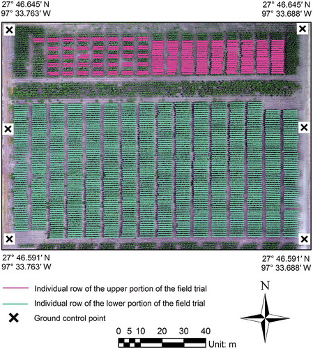
Before the growing season in 2016, an experimental maize field trial that consisted of two portions was established at the Texas A&M AgriLife Research and Extension Centre at Corpus Christi, TX (Figure 1). The upper (magenta) and lower (cyan) portions composed 108 and 448 genotypically different plots, respectively. Each plot consisted of two or four consecutive maize plant rows, and each delineated line represents an individual row. Rows without delineation depict hybrid fills or plots in the absence of height measurement in field surveys, and were excluded from analysis. The maize was planted on 1 April 2016, and was harvested on 5 August 2016.

Figure 1. The experimental maize field trial located at the Texas A&M AgriLife Research and Extension Centre in Corpus Christi, Texas.

2.2. Field measurement and UAS surveys

A ruler was used to measure the maize plant height. In an individual plot, the ground-measured height was presented by averaging measurements from three randomly selected plants. For the upper portion of the field trial, field surveys on height were conducted on 26 April, 13 May, 27 May, 6 June, and 1 July 2016, respectively. For the lower portion, ground height measurements were collected on 6 May, 13 May, 27 May, 6 June, and 1 July 2016, respectively.

Aerial images were acquired over the maize field trial during the growing season in 2016. Due to differences in platform availability and weather conditions at the field trial, multiple UAS platforms and imaging sensors were employed with flight frequency targeted weekly from 12 April to 15 July 2016. Because the focus was comparing UAS-SfM estimated canopy height against ground measurements, the five flights that were conducted closest to the corresponding ground surveys were selected for subsequent analysis (Table 1). Both DJI Phantom 4 and 3DR Solo platforms were quadcopters that focused on observing the field trial at or below 50 m above ground level (AGL) with travel speeds of 1 to 3 m s⁻¹. The fixed-wing senseFly eBee platform had a minimum cruise speed of 11 m s⁻¹ and was planned to fly over 100 m AGL to cover a larger area over the entire field complex.

Table 1. UAS flight information.

	Flight 1^a	Flight 2	Flight 3	Flight 4	Flight 5
Date	27 April 2016 (+1) 6 May 2016 (0)	17 May 2016 (+4)	26 May 2016 (−1)	8 June 2016 (+2)	30 June 2016 (−1)
UAS platform	DJI Phantom 4	DJI Phantom 4	senseFly eBee	3DR Solo	DJI Phantom 4
Flight height (m)	50 30	40	101	30	20
Camera model	DJI FC330	DJI FC330	Canon PowerShot S110	GoPro HERO3+ Black	DJI FC330
Size of image array (pixel)	4000 × 3000	4000 × 3000	4048 × 3048	4000 × 3000	4000 × 3000
GSD (mm pixel^−1)	23.3 13.7	19.1	38.4	20.0	7.7
Point density (points m^−2)	764.5 1333.4	686.1	81.6	865.1	5995.1

^aThe flight dates of the upper and lower portions of the field differed.

Flight 1 in Table 1 provides two individual flight dates for the upper and lower field portions to accommodate the availability of field surveys, and consequently produced two sets of values in terms of flight height, ground sample distance (GSD), and point density, respectively. The number parenthesized after an individual flight date indicates the day difference to its nearest ground survey date. A positive or negative sign reflects that the flight was conducted after or before its closest ground survey.

All the UAS flights were designed to target at least 65% sidelap and 80% frontlap. Before the maize was planted in the season, ground control targets (GCTs) were installed and surveyed in centimetre accuracy via virtual reference station (VRS) network around the field trial to geo-rectify the 2D and 3D geospatial products.

2.3. Canopy height model extraction

After each flight, aerial images were loaded into the Pix4Dmapper Pro (Pix4D SA, Lausanne, Switzerland) to perform SfM photogrammetric processing. A canopy height model (CHM) can be generated by differentiating the digital surface model (DSM) of an in-season flight from the digital elevation model (DEM) derived before the growing season. Although this study employed multiple UAS platforms and imaging sensors, it is worth noting that the bundle block adjustment (BBA) used in the SfM processing was able to calibrate the intrinsic camera parameters and to rectify the lens distortions across the various sensors.

2.4. Characterization of canopy height

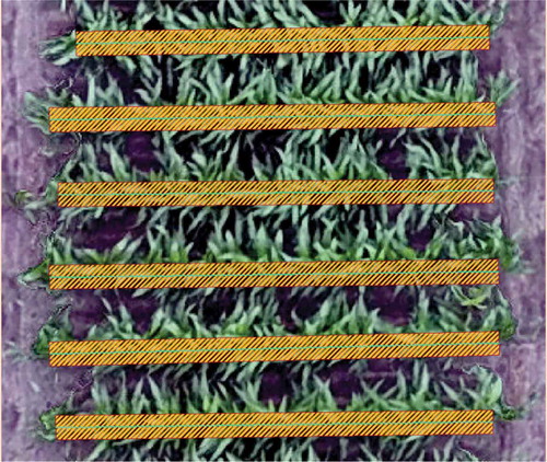
Crop row polygons (CRPs) along the maize rows were designed to facilitate estimating the canopy height. In order to generate an individual CRP, centrelines (cyan lines in Figure 2) that covered complete rows of maize plants were manually drawn on a georeferenced orthomosaic image. Then the width of the centrelines was inflated to a predefined number to form the polygons (orange in Figure 2). Canopy height was estimated by using height information in each polygon.

Figure 2. Crop row polygons superimposed on six consecutive maize rows at the lower portion of the field trial. The crop row polygons are inflated with adjustable width from the cyan centrelines, and the canopy height is estimated using the height information within the polygons.

After setting up the CRPs, the maize crop height was characterized and assessed by investigating height-dependent factors.

(1) The CRP width is adjustable in accordance with appearance and shape of different types of crops. Since the maize plants have sharp cone-shaped profile, the height estimation results were anticipated to be sensitive to the CRP width. Therefore, various CRP widths and percentile heights were examined to find the optimal combinations in the particular study for calculating the maize height.

(2) Height results were computed and compared between using the pixels in CRPs from the CHM raster and directly from the 3D point cloud data. In the literature, most UAS photogrammetry studies estimated the plant height based on rasterized CHM pixels, yet the similarity by using point cloud data remains unquantified. In this letter, height results extracted using point cloud data were compared against the results obtained from the rasterized CHM method.

(3) The canopy height estimation as a function of the DSM resolution was also examined. The purpose was to investigate impact of raster resolution on UAS-SfM height accuracy relative to field measurements. Coarser DSM resolutions can speed up computational loads for extracting crop growth analytics, particularly for large acreage crops, provided they are able to maintain favourable height estimation accuracy.

3. Results

3.1. Height estimate at varying CRP widths and percentiles

In order to compensate for plant dynamic movement due to wind and false parallax, various CRP widths were tested, covering from 5 to 60 cm with 5 cm increment. In addition, multiple percentile heights, from 50th to 99th, were computed using the pixels in each CRP from the CHM raster to examine the accuracy. The criterion to select the appropriate CRP width and percentile satisfies

(1)

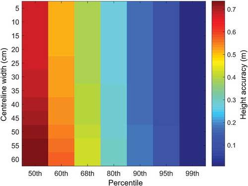
where d denotes the height difference in absolute value, H_i is the height of the i-th of n plots from ground survey, is the height of the i-th of n plots from UAS with p percentile and w CRP width, parameter space Ω_p = {50th, 60th, 68th, 80th, 90th, 95th, 99th}, and parameter space Ω_w = {5, 10, 15, ……, 50, 55, 60} in cm. Figure 3 presents height accuracy (i.e. UAS subtracted ground-measured height) at varying CRP widths and percentile heights for Flight 5 as indicated in Table 1. Results suggest that the height estimation accuracy improved when the percentile increases, and using 99th percentile outperformed lower percentiles in terms of maintaining height estimation accuracy. The 100th percentile height metric was not used here in order to avoid possible SfM artefacts that may introduce 3D structural spikes that contaminate height estimation.

Figure 3. Height accuracy (i.e. UAS-SfM subtracted ground-measured height) at varying CRP widths and percentile heights for Flight 5.

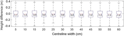
Focusing vertically on the 99th percentile column in Figure 3, detailed statistical distributions of height differences between UAS-SfM extraction and ground-measured truth are given in Figure 4. Each boxplot was calculated from a particular CRP width, and displays the distribution of height difference based on minimum (black horizontal line at the bottom), first quartile (lower blue horizontal line), median (red horizontal line), third quartile (higher blue horizontal line), and maximum (black horizontal line at the top) values. The numbers next to the median lines are mean values (unit: cm) for different CRP widths. Figure 4 indicates that while the interquartile ranges (IQRs) varied little across various CRP widths, the 20 and 25 cm CRP widths outperformed other widths in terms of the median value and full range of variation. Therefore, the maize height in this particular study should be estimated with the 99th percentile and 20 or 25 cm CRP width where the d value, as defined in Equation (1), is expected to produce the minimum value.

Figure 4. Boxplots showing the distribution of height difference between UAS-SfM and ground-measured truth at 99th percentile and varying CRP widths for Flight 5.

3.2. Height estimation with varying DSM resolutions and direct point cloud

Figure 5 shows the boxplot distributions of direct point cloud-based height subtracting DSM-based height with varying GSD resolutions at 25 cm CRP width and 99th percentile for Flight 2 (a) and Flight 4 (b). As indicated in Table 1, the GSDs of the orthomosaic images for Flight 2 and Flight 4 reached 2 cm pixel⁻¹, therefore, the rasterized DSMs were down-sampled from 2 cm through 24 cm for accuracy evaluation.

Figure 5. Boxplots showing the distribution of direct point cloud-based height subtracting DSM-based height with varying GSD resolutions at 25 cm CRP width and 99th percentile for Flight 2 (a) and Flight 4 (b).

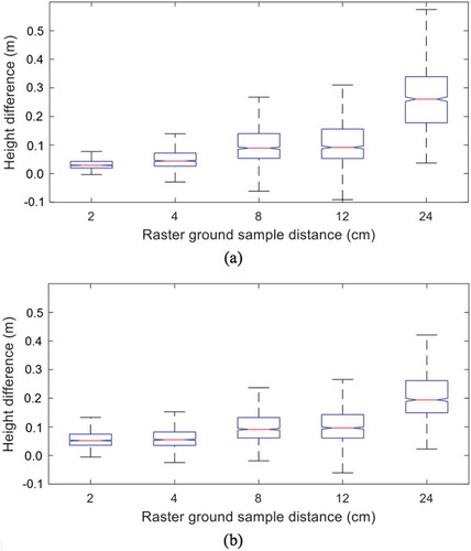
Results in Figure 5 reveal that the height differences between direct point cloud and DSM methods fall within 5 cm with decent IQR range when the DSM resolution was kept at its original 2 cm GSD. Meanwhile, the height difference tended to obtain a positive value, which means the heights calculated from the direct point cloud tended to be higher than DSM-based results. This is because in the DSM estimations the linear binning method that averages point clouds within a pixel was used. Figure 5 confirms that when the DSM pixel size grew larger the height fidelity, in general, deteriorated in comparison with the direct point cloud method in terms of the expected height difference and standard deviation. This is because at lower raster resolution the DSM appears relatively homogeneous by combining multiple parts of the plants and even bare soil within a single pixel. When the DSM had 24 cm pixel⁻¹ resolution, worse than 20 cm height difference was reached with nearly 20 cm IQR range.

The results also disclose that the DSM-based height estimation tended to degrade once the pixel resolution was greater than 12 cm. This finding can be of importance with regard to reducing the geospatial computing load without significantly losing height estimation accuracy, particularly for analysing large crop areas. DSM resolution values greater than 24 cm were not tested because of the width limit of individual CRPs (i.e., 25 cm as discussed earlier).

3.3. Height estimate over time

As discussed in previous subsections, selecting the 25 cm CRP width and 99th height percentile in this particular study outperforms other settings in terms of maintaining the fidelity of the UAS-extracted maize canopy height. Taking into consideration Figure 5 and the GSDs of orthomosaic images in Table 1, a uniform resolution of 4 cm pixel⁻¹ was used to ensure homogeneity among multiple flights. Figure 6 illustrates the UAS-extracted maize canopy height against field surveys across various dates for the field trial. Dots illustrated with different colours indicates height results obtained from different dates as described in Table 1 (i.e., Magenta: Flight 1 for the upper portion; Cyan: Flight 1 for the lower portion; Green: Flight 2; Blue: Flight 3; Black: Flight 4; and, Yellow: Flight 5). The red solid line indicates a linear regression model between UAS-SfM and ground-measured height.

Figure 6. UAS-SfM extracted maize canopy height against field measurement surveys. 25 cm CRP width, 99th height percentile and 4 cm/pixel CHM resolution was used to extract the UAS-SfM-based height.

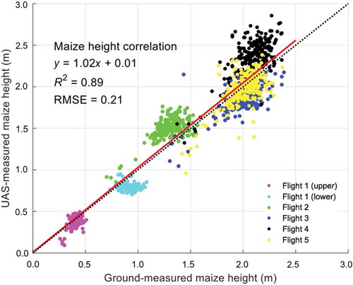
A height overestimate was observed in Figure 6 for the green and black dots (i.e., Flight 2 and Flight 4, respectively) because the flight experiments were performed a few days after the field measurement surveys and the plants would have grown. The slight underestimate from blue dots (i.e., Flight 3), on the contrary, originated primarily from the fact that the flight was conducted earlier than the ground height collection. However, the overall comparison results reveal that the regression line is close to the 1:1 relationship across the growing season (dashed black line) with the coefficient of determination (R²) = 0.89.

4. Conclusion

In this letter, canopy height in an experimental maize field was characterized based on UAS-SfM. The accuracy of various centreline widths, percentile height metrics, CHM versus point cloud data, and the impact of CHM resolution on estimation results were assessed. Results revealed that 1) 99th percentile with 25 cm CRP width provided the optimal accuracy for maize height estimation in this study environment; 2) the height difference between using rasterized DSM and direct point cloud was minor yet steadily increasing when the DSM resolution value grew; and 3) the accuracy of the DSM-based canopy height estimation dropped significantly after the DSM resolution became coarser than 12 cm. Results also suggested that the derived cost function, i.e. Equation (1), has the potential to be used for optimizing the height estimation accuracy of various crop types given ground truth.

Additional information

Funding

This work was supported by USDA Hatch Funds, Texas A&M AgriLife Research, and USDA-National Institute of Food and Agriculture [2014-68004-21836].

References

- Bendig, J., A. Bolten, S. Bennertz, J. Broscheit, S. Eichfuss, and G. Bareth. 2014. “Estimating Biomass of Barley Using Crop Surface Models (Csms) Derived from UAV-based RGB Imaging.” Remote Sensing 6 (11): 10395–10412. doi:10.3390/rs61110395.
- Çakir, R. 2004. “Effect of Water Stress at Different Development Stages on Vegetative and Reproductive Growth of Corn.” Field Crops Research 89 (1): 1–16. doi:10.1016/j.fcr.2004.01.005.
- Chen, R., T. Chu, J. A. Landivar, C. Yang, and M. M. Maeda. 2017. “Monitoring Cotton (Gossypium Hirsutum L.) Germination Using Ultrahigh-Resolution UAS Images.” Precision Agriculture 19 (1): 161–177. doi:10.1007/s11119-017-9508-7.
- Chu, T., R. Chen, J. A. Landivar, M. M. Maeda, C. Yang, and M. J. Starek. 2016. “Cotton Growth Modeling and Assessment Using Unmanned Aircraft System Visual-Band Imagery.” Journal of Applied Remote Sensing 10 (3): 036018. doi:10.1117/1.JRS.10.036018.
- Chu, T., M. J. Starek, M. J. Brewer, T. Masiane, and S. C. Murray. 2017b. “UAS Imaging for Automated Crop Lodging Detection: A Case Study over an Experimental Maize Field.” Autonomous Air and Ground Sensing Systems for Agricultural Optimization and Phenotyping II. SPIE 10218. doi:10.1117/12.2262812.
- Chu, T., M. J. Starek, M. J. Brewer, S. C. Murray, and L. S. Pruter. 2017a. “Assessing Lodging Severity over an Experimental Maize (Zea Mays L.) Field Using UAS Images.” Remote Sensing 9 (9): 923. doi:10.3390/rs9090923.
- Holman, F. H., A. B. Riche, A. Michalski, M. Castle, M. J. Wooster, and M. J. Hawkesford. 2016. “High Throughput Field Phenotyping of Wheat Plant Height and Growth Rate in Field Plot Trials Using UAV Based Remote Sensing.” Remote Sensing 8 (12): 1031. doi:10.3390/rs8121031.
- Malambo, L., S. C. Popescu, S. C. Murray, E. Putman, N. A. Pugh, D. W. Horne, G. Richardson, et al. 2018. “Multitemporal Field-Based Plant Height Estimation Using 3D Point Clouds Generated from Small Unmanned Aerial Systems High-Resolution Imagery.” International Journal of Applied Earth Observation and Geoinformation 64: 31–42. doi:10.1016/j.jag.2017.08.014.
- Pugh, N. A., D. Horne, S. Murray, G. Carvalho, L. Malambo, J. Jung, A. Chang, et al. 2018. “Temporal Estimates of Crop Growth in Sorghum and Maize Breeding Enabled by Unmanned Aerial Systems.” The Plant Phenome Journal 1 (1).
- Stanton, C., M. J. Starek, N. Elliott, M. Brewer, M. M. Maeda, and T. Chu. 2017. “Unmanned Aircraft System-Derived Crop Height and Normalized Difference Vegetation Index Metrics for Sorghum Yield and Aphid Stress Assessment.” Journal of Applied Remote Sensing 11 (2): 026035. doi:10.1117/1.JRS.11.026035.
- Tetila, E. C., B. B. Machado, N. A. de Souza Belete, D. A. Guimarães, and H. Pistori. 2017. “Identification of Soybean Foliar Diseases Using Unmanned Aerial Vehicle Images.” IEEE Geoscience and Remote Sensing Letters 14 (12): 2190–2194. doi:10.1109/LGRS.2017.2743715.
- Westoby, M. J., J. Brasington, N. F. Glasser, M. J. Hambrey, and J. M. Reynolds. 2012. “‘Structure-From-Motion’ Photogrammetry: A Low-Cost, Effective Tool for Geoscience Applications.” Geomorphology 179: 300–314. doi:10.1016/j.geomorph.2012.08.021.